1. Introduction
An Inertial Navigation System (INS) can provide a vehicle with the full navigation signals, such as position, velocity, attitude, etc., autonomously, but its error accumulates with time so that it cannot work alone with high accuracy for a long period. Therefore, the integration of the INS with others, such as the Global Navigation Satellite System (GNSS), has been investigated intensively (Chen et al., Reference Chen, Shen, Zhang, Tomizuka, Xu and Chiu2013). However, the GNSS signals are prone to jamming and/or spoofing unintentionally or intentionally. In contrast, Terrain-Aided Navigation (TAN), which has been successfully implemented for a cruise missile, an aircraft, an underwater vehicle and others, is totally autonomous (Kim et al., Reference Kim, Cho, Lee and Kang2015; Fountain, Reference Fountain1997; Melo and Matos, Reference Melo and Matos2017). Hence, TAN is crucial for a vehicle especially in a GNSS-denied environment.
A TAN system is usually composed of an INS, a sensor to measure the terrain elevation, a reference Digital Elevation Map (DEM) and a matching algorithm. If the INS, the elevation sensor and the reference DEM have been assembled in advance in the TAN system, the TAN performance is mainly dominated by the matching algorithm (Wang et al., Reference Wang, Zhu, Qin, Jiang and Li2018). The matching algorithms can be classified by the ways in which the samples are employed in the matching as the single-point, the one-dimensional (1D) sequence, the two-dimensional (2D) grey-value image and the three-dimensional (3D) elevation image (Wong, Reference Wong1978; Rodriguez and Aggarwal, Reference Rodriguez and Aggarwal1990; Sjanic and Gustafsson, Reference Sjanic and Gustafsson2015; Venable and Raquet, Reference Venable and Raquet2016; Sattler et al., Reference Sattler, Leibe and Kobbelt2017; Xiong and Xie, Reference Xiong and Xie2017). Since the 2D and the 3D image matching algorithms use more samples in the matching than the former two, they usually match more accurately and stably than the former two. Furthermore, the 3D elevation image matching algorithm is superior to that of the 2D image in terms of both the sensitivity to the fluctuation of elevation in a region, and the robustness to cloud, brightness and so on. Therefore, this paper will focus on the matching using a 3D elevation image.
Since the only difference between a 2D and a 3D image is their pixel value, the typical 2D image matching algorithms, such as the Normalised Product Correlation (NPC) (Wong and Hall, Reference Wong and Hall1978), the corner-/edge-detector based (Harris and Stephens, Reference Harris and Stephens1988) and the invariant-feature based (Lowe, Reference Lowe2004), can also be employed by the 3D image matching algorithms. Compared with the correlation algorithms and the corner-/edge-detector-based algorithms, the invariant-feature-based matching algorithms are invariant to rotation, scaling and translation (Lowe, Reference Lowe2004; Ren and Chang, Reference Ren and Chang2014; Hu, Reference Hu1962; Canterakis, Reference Canterakis1999). Moreover, they are also robust to noise, which is beneficial for matching with the noisy 3D elevation image especially. Hence, the invariant-feature-based algorithms have been intensively investigated in recent years.
Particularly, since the Zernike Moments (ZMs) are not only orthogonal but also extendable to the infinite orders, they offer the superior discrimination power and noise resistence to Hu moments and other invariant features (Novotni and Klein, Reference Novotni and Klein2004). Hence, the ZMs have been employed widely in pattern recognition, image retrieval and so on (Clemente et al., Reference Clemente, Pallotta, De Maio, Soraghan and Farina2015; Millan et al., Reference Millan, Dempere-Marco, Pozo, Cebral and Frangi2007; Venkatraman et al., Reference Venkatraman, Chakravarthy and Kihara2009; Grandison et al., Reference Grandison, Roberts and Morris2009; Yan et al., Reference Yan, Zhang, Tian and Gao2016). The 3D ZMs have also been proposed to design a terrain-matching algorithm, but the biggest barrier to the implementation of the algorithm in real time is its huge computational load (Wu and Ye, Reference Wu and Ye2008; Ye and Chen, Reference Ye and Chen2012). Even though some methods have been proposed to compute the 3D ZMs efficiently (Hosny and Hafez, Reference Hosny and Hafez2012; Pozo et al., Reference Pozo, Villa-Uriol and Frangi2011; Al-Rawi, Reference Al-Rawi2012), they may be invalid for the 3D terrain surface since they are designed for the 3D entity. Considering the fact that most of the computation is consumed by computing the 3D ZMs of the reference DEMs, an efficient algorithm has been proposed by computing the 3D ZMs of the reference DEMs using a circular template offline in advance, which provides an opportunity for the implementation of the 3D ZMs algorithm in real time (Wang et al., Reference Wang, Zhu, Gao and Wang2019). Moreover, the 3D ZMs of the terrain surface have the items unrelated to elevation which are redundant with the matching algorithm. It has been found that only the even orders of the 3D ZMs have the redundant items. Hence, we have proposed the matching algorithm by excluding the even-order 3D ZMs from the descriptors (Wang et al., Reference Wang, Zhu, Gao and Wang2019). However, not all of the even-order 3D ZMs have the redundant items. If the even-order 3D ZMs without the redundant items are added into the matching algorithm composed of the only odd-order 3D ZMs, the matching performance should be improved further, which will be addressed in this paper. The rest of the paper is organised as follows. The terrain matching algorithm based on the 3D ZMs will be briefly presented in Section 2. In Section 3, the redundant items in the even-order 3D ZMs will be detailed before the revised descriptors are proposed for the new matching algorithm. In Section 4, the performance of the algorithm with the revised descriptors will be demonstrated by simulations. In Section 5, the conclusions will be drawn finally.
2. 3D-ZM-based terrain matching algorithm
The terrain matching algorithm based on the 3D ZMs is briefed herein. More details can be found from Novotni and Klein (Reference Novotni and Klein2004).
The 3D ZM of a DEM,
 $\Omega _{n,l}^m$
, is defined as
 $$\Omega _{n,l}^m = {3 \over {4\pi }}\sum\limits_{r + s + t \le n} {\overline {\chi _{n,l,m}^{r,s,t}} } {M_{r,s,t}}$$
where
 $n$
,
 $l$
and
 $m$
are integers, and
 $r$
,
 $s$
and
 $t$
are nonnegative integers,
 $n \in [0,Max]$
,
 $l \in [0,n]$
,
 $m \in [ - l,l]$
,
 $Max$
is the maximal order of the moment, and
 $(n - l)$
must be an even nonnegative integer;
 $\chi _{n,l,m}^{r,s,t}$
is the combinatorial coefficient;
 $\overline {\chi _{n,l,m}^{r,s,t}} $
is the complex conjugate of
 $\chi _{n,l,m}^{r,s,t}$
; and
 ${M_{r,s,t}}$
is the geometric moment which is defined as
 $${M_{r,s,t}} = \int_{\left| {\bf{x}} \right| \le 1} {f\left( {\bf{x}} \right){x^r}{y^s}{z^t}} {\rm{d}}{\bf{x}}$$
where
 ${\bf{x}} = {\left( {x,y,z} \right)^{\rm{T}}}$
. Here,
 $$f\left( {\bf{x}} \right) = \left\{ {\matrix{ {\matrix{ {{\rm{1,}}} & {{\bf{x}} \in {\bf{S}}} \cr } } \cr {\matrix{ {0,} & {{\bf{x}} \notin {\bf{S}}} \cr } } \cr } } \right.$$
where
 ${\bf{S}}$
is the point set of the terrain surface. If there are
 $N$
samples on the surface
 ${\bf{S}}$
in the normalised coordinate and the
 $i$
th sample
 ${{\bf{x}}_i} = {\left( {{x_i},{y_i},{z_i}} \right)^{\rm{T}}}$
, then
 ${M_{r,s,t}}$
in Equation (2) can be discretised as
 $${M_{r,s,t}} = \sum\limits_{i\,=\,1}^N {x_i^ry_i^sz_i^t} $$
The 3D ZM
 $\Omega _{n,l}^m$
is not invariant to rotation, so the following 3D Zernike descriptor
 ${F_{n,l}}$
, the norm of the vector composed of the 3D ZMs, is further constructed as
 $${F_{n,l}} = \left\| {{{\left[ {\Omega _{n,l}^l,\;\Omega _{n,l}^{l - 1}, \cdots, \Omega _{n,l}^{ - l}} \right]}^{\rm{T}}}} \right\|$$
In a matching, the multiple descriptors are usually employed to construct a feature vector to improve both the discrimination power and the robustness of the matching algorithm. The existing feature vector
 ${\boldsymbol{F}}$
with the maximal order of
 $L$
is defined as
 $${\boldsymbol{F}} = {\left[ {\matrix{ {{F_{{\rm{0}},0}}} & {{F_{{\rm{1}},{\rm{1}}}}} & {{F_{{\rm{2}},0}}} & \cdots & {{F_{L,L}}} \cr} } \right]^{\rm{T}}}$$
Since both
 ${F_{0,0}}$
and
 ${F_{1,1}}$
are unrelated to elevation, the feature vector
 ${\boldsymbol{F}}$
should be revised as
 $${\boldsymbol{F}} = {\left[ {\matrix{ {{F_{{\rm{2}},0}}} & {{F_{{\rm{2}},{\rm{2}}}}} & {{F_{{\rm{3}},1}}} & \cdots & {{F_{L,L}}} \cr } } \right]^{\rm{T}}}$$
As pointed out by Wang et al. (Reference Wang, Zhu, Gao and Wang2019), the matching performance cannot be improved further by enlarging the maximal order
 $L$
if
 $L$
is no less than 10. Hence,
 $L$
is set as 10 hereinafter.
In the matching algorithm, both the feature vector of a Real-time Elevation Map (REM) and that of a candidate DEM are calculated first. Then, the similarity of the feature vector of the REM to that of the candidate DEM is evaluated by a criterion. Herein, the criterion is the Canberra distance which is defined as
 $$d\left( {{\boldsymbol{p}},{\boldsymbol{q}}} \right) = \sum\limits_{h = 1}^K {\left| {{{{p_h} - {q_h}} \over {{p_h} + {q_h}}}} \right|} $$
where
p
and
q
are the two K-dimensional vectors and
 ${p_h} + {q_h} \ne {\rm{0}}$
.
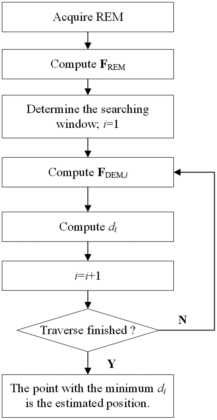
Figure 1 presents the procedure of the matching. In Figure 1,
 ${{\boldsymbol{F}}_{{\rm{REM}}}}$
,
 ${{\boldsymbol{F}}_{{\rm{DEM,}}i}}$
and
 ${d_i}$
are the feature vector of the REM, the feature vector of the reference DEM at the ith grid point in the search window, and the Canberra distance between
 ${{\boldsymbol{F}}_{{\rm{REM}}}}$
and
 ${{\boldsymbol{F}}_{{\rm{DEM,}}i}}$
, respectively. After the search window in the reference DEM is traversed, the estimated position will be the point with the minimal Canberra distance.
Procedure of the terrain-matching algorithm.

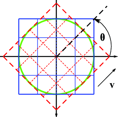
To reduce the impact of rotation on the matching performance, a circular template illustrated in Figure 2 is employed in the matching. In Figure 2, if a vehicle moves along the direction v, the REM overlaps with the reference DEM totally in the circular template even though there is a heading angle
 $\theta $
.
Circular template employed for both REM and DEM.

In this paper, the DEMs are acquired from the Advanced Spaceborne Thermal Emission and Reflection Radiometer Global Digital Elevation Model (ASTER GDEM). An REM is sampled from the DEM by the bilinear interpolation.
3. 3D ZMs algorithm with revised descriptors
Although both
 ${F_{0,0}}$
and
 ${F_{1,1}}$
are excluded in Equation (7), there are still the redundant items in the even-order descriptors as analysed by Wang et al. (Reference Wang, Zhu, Gao and Wang2019). Since there are no redundant items in the odd-order descriptors, a matching algorithm with the odd-order descriptors has been proposed. However, it should be noted that not all the even-order descriptors have the redundant items. Hence, if the even-order descriptors with the elevation-related items are also included in the feature vector, the matching performance of the algorithm should be improved further, which will be investigated herein.
3.1 Redundant items in even-order 3D ZMs
According to Novotni and Klein (Reference Novotni and Klein2004), Equation (1) can also be rewritten as
 $$\Omega _{n,l}^m = {3 \over {4\pi }}\sum\limits_{r + s + t \le n} {\overline {Z_{n,l}^m\left( {\bf{x}} \right)} } $$
where
 $\overline {Z_{n,l}^m\left( {\bf{x}} \right)} $
is the complex conjugate of the 3D Zernike function
 $Z_{n,l}^m\left( {\bf{x}} \right)$
. In the spherical coordinate, the 3D Zernike function
 $Z_{n,l}^m\left( {\bf{x}} \right)$
can be rewritten as
 $$Z_{n,l}^m\left( {\rho, \theta, \varphi } \right) = {R_{n,l}}\left( \rho \right)Y_l^m\left( {\theta, \varphi } \right)$$
where
 $\left( {\rho, \theta, \varphi } \right)$
is the spherical coordinate of
 ${\bf{x}}$
,
 ${R_{n,l}}\left( \rho \right)$
is the radial function and
 $Y_l^m\left( {\theta, \varphi } \right)$
is the spherical harmonic function;
 $$\rho = \sqrt {{x^2} + {y^2} + {z^2}} $$
 $${R_{n,l}}\left( \rho \right) = \sum\limits_{g = 0}^{{{n - l} \over 2}} {{k_g}{\rho ^{l + 2g}}} $$
 $$Y_l^m\left( {\theta, \varphi } \right) = \sqrt {{{2l + 1} \over {4\pi }}{{\left( {l - m} \right)!} \over {\left( {l + m} \right)!}}} P_l^m\left( {\cos \theta } \right){e^{jm\varphi }}$$
where
 $P_l^m\left( x \right)$
is the associated Legendre polynomial of
 $x$
and
 ${j^2} = - 1$
. There is
 $$P_l^m\left( x \right) = {\left( {1 - {x^2}} \right)^{{m \over 2}}}P_l^{\left( m \right)}\left( x \right)$$
 $$P_l^{ - m}\left( x \right) = {\left( { - 1} \right)^m}{{\left( {l - m} \right)!} \over {\left( {l + m} \right)!}}P_l^m\left( x \right)$$
where
 $P_l^{\left( m \right)}\left( x \right)$
is the m-order derivative of the Legendre polynomial
 ${P_l}\left( x \right)$
:
 $$P_l^{\left( m \right)}\left( x \right) = \sum\limits_{h = 0}^{\left\lfloor {{{l - m} \over 2}} \right\rfloor } {{k_h}{x^{l - m - 2h}}} $$
where
 $\left\lfloor x \right\rfloor $
is the floor function of
 $x$
. Substituting Equations (11)–(15) into Equation (10) yields
 $$Z_{n,l}^m\left( {\bf{x}} \right) = \sqrt {{{2l + 1} \over {4\pi }}{{\left( {l - m} \right)!} \over {\left( {l + m} \right)!}}} \left( {\sum\limits_{h = 0}^{\left\lfloor {{{l - m} \over 2}} \right\rfloor } {{k_h}{\rho ^{{\rm{2}}h}}{z^{l - m - 2h}}} } \right)\left( {\sum\limits_{g = 0}^{{{n - l} \over 2}} {{k_g}{\rho ^{2g}}} } \right){\left( {x + jy} \right)^m}$$
In Equation (17), if
 $l - m - 2h\,=\,0$
, the 3D Zernike function
 $Z_{n,l}^m\left( {\bf{x}} \right)$
will possibly contain the items unrelated to elevation. Considering that
 $n - l$
is an even nonnegative integer,
 $n$
,
 $l$
and
 $m$
should have the same parity. When
 $2h = l - m$
, Equation (17) can be rewritten as
 $$Z_{n,l}^m\left( {{\bf{x}},\,\,h} \right) = {k_h}\sqrt {{{2l + 1} \over {4\pi }}{{\left( {l - m} \right)!} \over {\left( {l + m} \right)!}}} \left[ {\sum\limits_{g = 0}^{{{n - l} \over 2}} {{k_g}{{\left( {{x^2} + {y^2} + {z^2}} \right)}^{g + h}}} } \right]{\left( {x + jy} \right)^m}$$
Additionally, there is an identically changing formula
 $${\left( {{x^2} + {y^2} + {z^2}} \right)^n} = {\left( {{x^2} + {y^2}} \right)^n} + \sum\limits_{k\,=\,1}^n {C_n^k{{\left( {{x^2} + {y^2}} \right)}^{n - k}}\,{z^{2k}}} $$
where
 $C_n^k$
is the combinatorial number.
Then, if the items containing
 $z$
are discarded from Equation (18), the remaining part, which is also called the redundant items, can be described as
 $$Z_{n,l}^m\left( {x,y,h} \right) = {k_h}\sqrt {{{2l + 1} \over {4\pi }}{{\left( {l - m} \right)!} \over {\left( {l + m} \right)!}}} \left[ {\sum\limits_{g = 0}^{{{n - l} \over 2}} {{k_g}{{\left( {{x^2} + {y^2}} \right)}^{g + h}}} } \right]{\left( {x + jy} \right)^m}$$
In Equation (20), the parity of the powers of
 $x$
and
 $y$
is determined by the item
 ${\left( {x + jy} \right)^m}$
or
 $m$
only.
If
 $m$
is an odd integer, all the items of
 ${\left( {x + jy} \right)^m}$
are odd with respect to
 $x$
and/or
 $y$
for a circular template. Since
 $x$
,
 $y$
and
 $z$
have been centralised and normalised, the sum of
 $Z_{n,l}^m\left( {x,y,h} \right)$
in Equation (9) is zero so that the items unrelated to elevation have no impact on the 3D ZMs. That is, there are no redundant items in the odd-order 3D ZMs, which is consistent with the analysis by Wang et al. (Reference Wang, Zhu, Gao and Wang2019).
In contrast, if
 $m$
is an even-nonnegative integer, there may be redundant items in the 3D ZMs. That is, the sums of the items unrelated to elevation may not be zero, which will be analysed in the following two cases.
Case 1:
 $m\,=\,4a$
and
 $a$
is a nonnegative integer. If
 $m\,=\,0$
, the value of
 ${\left( {x + jy} \right)^m}$
is 1 so that the sum of
 $Z_{n,l}^m\left( {x,y,h} \right)$
is not zero. If
 $m\,=\,4$
, there is
 $${\left( {x + jy} \right)^4} = {x^4}\,+\,4j{x^3}y - 6{x^2}{y^2} - 4jx{y^3} + {y^4}$$
In a circular template, the sum of
 ${\left( {x + jy} \right)^{\rm{4}}}$
can be calculated as
 $$\sum\limits_{i\,=\,1}^N {{{\left( {{x_i} + j{y_i}} \right)}^4}} = \sum\limits_{i\,=\,1}^N {\left( {x_i^4 - 6x_i^2y_i^2{\rm{ + }}y_i^4} \right)} $$
That is, the sum of
 $Z_{n,l}^m\left( {x,y,h} \right)$
is also not zero. Similarly, the sum of
 $Z_{n,l}^m\left( {x,y,h} \right)$
is not zero either if
 $m\,=\,4a$
and
 $m\,\gt \,4$
. Hence, there are the nonzero items unrelated to elevation in the 3D ZMs if
 $m\,=\,4a$
. The nonzero items are redundant with the 3D ZMs.
Case 2:
 $m\,=\,4a\,+\,2$
. If
 $m = {\rm{2}}$
, the sum of
 ${\left( {x + jy} \right)^{\rm{2}}}$
can be calculated as
 $$\sum\limits_{i\,=\,1}^N {{{\left( {{x_i} + j{y_i}} \right)}^{\rm{2}}}} = \sum\limits_{i\,=\,1}^N {\left( {x_i^{\rm{2}}\,+\,2{x_i}{y_i} - y_i^{\rm{2}}} \right)} \,=\,0$$
That is, the sum of
 $Z_{n,l}^m\left( {x,y,h} \right)$
is zero. Similarly, the sum of
 $Z_{n,l}^m\left( {x,y,h} \right)$
is also zero if
 $m\,=\,4a\,+\,2$
and
 $m \gt {\rm{2}}$
. Hence, the items unrelated to elevation are zeros in the 3D ZMs if
 $m\,=\,4a\,+\,2$
. These items have no impact on the 3D ZMs.
In all, there are the redundant items in the even-order 3D ZMs only when
 $m\,=\,4a$
.
3.2 Correlation of 3D ZMs with elevation
In the terrain matching, a region is discriminated from others by its fluctuation of elevation. In the region with the large fluctuation, the modules of the 3D ZMs are also large. In contrast, the modules of the 3D ZMs approach zero in the flat region. In addition, a larger fluctuation of the region results in a greater standard deviation of the region’s elevation, and vice versa. Hence, the modules of the 3D ZMs should correlate positively with the standard deviations of the regions’ elevation if there are no redundant items in the 3D ZMs. However, the redundant items in the 3D ZMs will have an impact on the correlation between the modules of the 3D ZMs and the standard deviations of the regions’ elevation significantly. The modules of the 3D ZMs with the redundant items may even correlate negatively with the standard deviations of the regions’ elevation, which will have a negative impact on the matching performance. Hence, it is necessary to investigate on the correlation between the 3D ZMs and the standard deviation of the regions’ elevation further, which will be addressed herein.
As many as 5,484 DEMs are acquired from the ASTER GDEM data without intersection for the following correlation statistically. The resolution and the size of the DEMs are 30 m/grid and 80 grids × 80 grids, respectively. In each DEM, the modules of the 3D ZMs are calculated in the circular template illustrated in Figure 2. Since
 $\Omega _{n,l}^{ - m} = {\left( { - 1} \right)^m}\overline {\Omega _{n,l}^m} $
,
 $\left\| {\Omega _{n,l}^{ - m}} \right\| = \left\| {\Omega _{n,l}^m} \right\|$
so that only the 3D ZMs with
 $m \ge {\rm{0}}$
will be considered. There are 161 modules of the 3D ZMs with
 $m \ge {\rm{0}}$
in total when the maximal order of the 3D ZMs is 10. Since there are ten 3D ZMs, such as
 $\Omega _{0,0}^0$
,
 $\Omega _{{\rm{1,1}}}^{\rm{0}}$
,
 $\Omega _{{\rm{1,}}\,{\rm{1}}}^{\rm{1}}$
, etc., unrelated to elevation, the remaining 151 modules will be analysed herein. At the same time, the standard deviation of the DEM’s elevation in the circular template is calculated.
Figure 3 depicts the correlation between the modules of the 3D ZMs and the standard deviations of the DEMs’ elevation. In Figure 3, most of the modules of the 3D ZMs positively correlate with the standard deviations of the DEMs’ elevation, but there are some modules of the 3D ZMs that exhibit negative correlation with the standard deviations of the DEMs’ elevation. The coefficients of the even-order 3D ZMs with
 $m\,=\,4a$
are shown in red, while the others are shown in blue. All the 3D ZMs, without exception, whose modules are negatively correlated with the standard deviations of the DEMs’ elevation, are the even order and
 $m\,=\,4a$
, which coincides with the above analysis. Hence, the even-order 3D ZMs with
 $m\,=\,4a$
should be excluded from the descriptors.
Correlation between the modules of the 3D ZMs and the standard deviations of the DEMs’ elevation.

3.3 3D ZMs algorithm
If the even-order 3D ZMs with
 $m\,=\,4a$
are excluded from the descriptors, Equation (5) can be rewritten as
 $$N{F_{n,l}} = \left\{ \matrix{ \left\| {{{\left[ {\Omega _{n,l}^l,\;\Omega _{n,l}^{l - 1},\, \cdots, \Omega _{n,l}^{ - l}} \right]}^{\rm{T}}}} \right\|,n = 2i + 1; \hfill \cr \left\| {{{\left[ {\Omega _{n,l}^l,\;\Omega _{n,l}^{l - 1}, \,\cdots, \Omega _{n,l}^1,\Omega _{n,l}^{ - 1},\, \cdots, \Omega _{n,l}^{ - l}} \right]}^{\rm{T}}}} \right\|,n = 2i,m \ne 4a \hfill \cr} \right.$$
where
 $N{F_{n,l}}$
is the revised descriptor and
 $i\,=\,1,2,3, \cdots $
. If
 $l\,=\,0$
and the order
 $n$
is even,
 $m = {\rm{0}}$
, but
 $\Omega _{n,{\rm{0}}}^{\rm{0}}$
is excluded. That is,
 $N{F_{n,{\rm{0}}}}$
should not be included in the feature vector since it is null. Hence, the new feature vector with the revised descriptors,
 ${\boldsymbol{NF}}$
, can be written as
 $${\boldsymbol{NF}} = {\left[ {\matrix{ {N{F_{{\rm{2}},2}}} & {N{F_{3,1}}} & {N{F_{{\rm{3}},3}}} & \cdots & {N{F_{L,L}}} \cr } } \right]^{\rm{T}}}$$
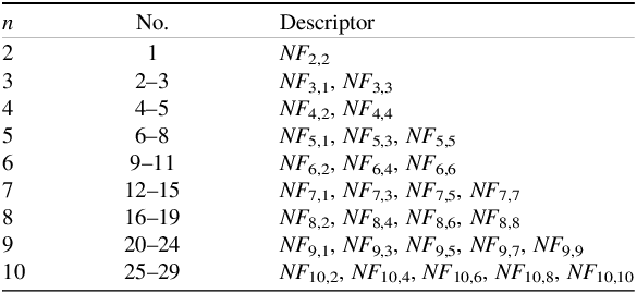
As listed in Table 1, there are 29 revised descriptors in total when the maximal order is 10. Compared with the feature vector in Equation (7), the 3D ZMs with the redundant items are excluded from the new feature vector in Equation (25). Hence, the new algorithm with the feature vector in Equation (25) should achieve a better matching performance than that with the feature vector in Equation (7), which will be verified by the numerical experiments in the following section.
Descriptors with the maximal order of 10

The new descriptor,
 $N{F_{n,l}}$
, also retains the rotational invariance. Compared with
 ${F_{n,l}}$
, the key difference lies in the removal of all redundant terms
 $\Omega _{even,even}^{4a}$
, which eliminates the adverse impact of the elevation-independent information on the descriptor. The removed redundant items for the new descriptors also save the computational load to some extent. The improved descriptor’s accuracy and reliability in terrain matching will be validated and analysed in the numerical experiments presented in the next section.
4. Numerical experiments
Since the feature vector is composed of the revised descriptors in Equation (25), the matching performance is dominated by the revised descriptors accordingly. The performance of the revised descriptors, including their discrimination power and the impact of noise and rotation, can be investigated in the same way as that employed by Wang et al. (Reference Wang, Zhu, Gao and Wang2019), which will not be addressed herein any more. In the following, the algorithm with the revised descriptors in Equation (25) (‘Algorithm C’) will be compared with that with all the 34 existing descriptors (‘Algorithm A’) and that with the 14 odd-order descriptors (‘Algorithm B’) by the numerical experiments.
The numerical experiments are implemented in the two typical DEMs shown in Figure 4, Map A and Map B. The standard deviations of elevation are 57.86 m on Map A and 197.41 m on Map B. Therefore, Map A is flatter than Map B so that the adaptability of the three algorithms can be evaluated to some extent. The two maps have a resolution of 30 m/grid and a size of 300 grids × 300 grids. The REMs are sampled from the two DEMs. The zero-mean Gaussian noises with the standard deviations of 5.8 and 19.7 m are added to Map A and Map B, respectively. The standard deviations of the noises are approximately 10% of σ (the standard deviations of the two maps’ elevations). The heading angles of 0°, 5°, 45° and 75° between the REMs and the reference DEMs are applied. The size of the REMs is 80 grids × 80 grids, but the circular template illustrated in Figure 2 is still employed in the calculation as mentioned above. The performance of the three algorithms will be evaluated by their matching success rates quantitatively. Considering the heading angles between the REMs and the DEMs, as illustrated in Figure 2, the matching is judged as success if the two horizontal matching errors, both
 ${e_x}$
and
 ${e_y}$
, are less than 1.4 grid (the diagonal distance of a grid). The three algorithms will be run for 1,000 times independently and randomly for each heading angle to compute the matching success rate statistically.
3D images of the two maps.

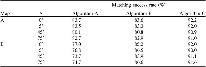
Table 2 lists the matching results with the three algorithms in the two maps. As expected, the algorithm with the revised descriptors, Algorithm C, achieves the highest matching success rate even though there is the impact of noise and rotation. In the two maps, the matching success rate of Algorithm C is no less than 90%. Although the algorithm with all the 34 existing descriptors, Algorithm A, has almost the same matching success rate as that with the 14 odd-order descriptors, Algorithm B, in Map A, its matching success rate is far less than the latter in Map B. That is, the 20 existing even-order descriptors employed in Algorithm A not only increase the computational load significantly but also degrade the matching success rate. It is also noted that the matching success rate of Algorithm B is no greater than 81% in Map A if the heading angle is 45°. Hence, the matching performance using the odd-order descriptors should be improved further. In contrast, Algorithm C, which includes the 15 revised even-order descriptors, demonstrates a substantial increase in the matching success rate, even in the challenging environments such as the flat region Map B. As listed in Table 2, the matching success rates of Algorithm C are no less than 90% even though there are both strong noise and a large heading angle in the two maps, which demonstrates its robustness to noise and rotation.
Matching success rate

5. Conclusion
Aiming at improving the matching performance with the 3D ZMs, the redundant items in the even-order 3D ZMs are investigated intensively. It is found that the even-order 3D ZMs have the redundant items unrelated to elevation when
 $m\,=\,4a$
. The correlation between the modules of the 3D ZMs and the standard deviations of elevation indicate the impact of the redundant items on the even-order 3D ZMs. A new matching algorithm with the revised descriptors is proposed. In the revised descriptors, the even-order 3D ZMs with the redundant items are excluded from the even-order descriptors, while the odd-order descriptors remain unchanged. The numerical experiment results demonstrate that the algorithm with the revised descriptors achieves the matching success rate no less than 90% in the two maps even though there is the impact of noise and rotation.
Acknowledgements
The digital elevation model data are downloaded from Geospatial Data Cloud site, Computer Network Information Center, Chinese Academy of Sciences. (http://www.gscloud.cn). The work is sponsored by National Nature Science Foundation of China under the grant number 62173011.
Competing interests
The authors declare that they have no known competing financial interests or personal relationships that could have appeared to influence the work reported in this paper.