1 Introduction
The presence of surface heterogeneities has the potential to significantly alter the properties of a turbulent boundary layer. If the surface varies in the direction orthogonal to the flow direction, secondary flows can form, comprised of swirling fluid motion in the plane normal to the primary flow direction. Although the effects of surface conditions are typically assumed to be confined to the near-wall roughness layer (Castro Reference Castro2007; Flack & Schultz Reference Flack and Schultz2014), secondary motions are known to significantly modify the mean velocity profile of the primary flow as well as the turbulence properties throughout the boundary layer (Medjnoun, Vanderwel & Ganapathisubramani Reference Medjnoun, Vanderwel and Ganapathisubramani2018). Secondary flows have been observed experimentally over the irregular surface of a damaged turbine (Barros & Christensen Reference Barros and Christensen2014), over surfaces with streamwise-aligned ridges (Vanderwel & Ganapathisubramani Reference Vanderwel and Ganapathisubramani2015), over surfaces with streamwise-aligned strips of roughness (Bai et al. Reference Bai, Hutchins and Monty2018) and over herringbone patterned riblet surfaces (Kevin et al. Reference Kevin, Monty, Bai, Pathikonda, Nugroho, Barros, Christensen and Hutchins2017). There have also been significant recent numerical studies to understand the formation of these secondary motions due to spanwise heterogeneous surfaces (see e.g. Goldstein & Tuan Reference Goldstein and Tuan1998; Türk et al. Reference Türk, Daschiel, Stroh, Hasegawa and Frohnapfel2014; Willingham et al. Reference Willingham, Anderson, Christensen and Barros2014; Anderson et al. Reference Anderson, Barros, Christensen and Awasthi2015; Stroh et al. Reference Stroh, Hasegawa, Kriegseis and Frohnapfel2016). A good summary of the corresponding contributions is given by Hwang & Lee (Reference Hwang and Lee2018).
Originally classified by Prandtl (Reference Prandtl1952), secondary flows can form as a result of centrifugal forces in curved channels, known as Prandtl’s first kind, or as a result of Reynolds stress gradients, which are known as turbulence-driven or Prandtl’s second kind (Bradshaw Reference Bradshaw1987; Nezu Reference Nezu2005). For straight, open channel or turbulent boundary layer flows, centrifugal forces are not present but surface heterogeneities can create inhomogeneities in the Reynolds stress components which lead to the formation of these turbulence-driven secondary flows of the second kind (Anderson et al. Reference Anderson, Barros, Christensen and Awasthi2015). Similar turbulence-driven secondary flows can also form in duct flows, where it has been shown that the mean secondary flow is related to an inhomogeneous probability distribution of coherent flow structures (Uhlmann et al. Reference Uhlmann, Pinelli, Kawahara and Sekimoto2007; Pinelli et al. Reference Pinelli, Uhlmann, Sekimoto and Kawahara2010; Kawahara, Uhlmann & Van Veen Reference Kawahara, Uhlmann and Van Veen2012), especially for marginally turbulent flows at low Reynolds numbers. For turbulent duct flows at low Reynolds numbers it has additionally been shown that the turbulence-driven secondary flow can be captured through exact coherent states (Uhlmann, Kawahara & Pinelli Reference Uhlmann, Kawahara and Pinelli2010; Kawahara et al. Reference Kawahara, Uhlmann and Van Veen2012; Okino & Nagata Reference Okino and Nagata2012).
The secondary flows formed in boundary layers are far away from a marginally turbulent state. In turbulent boundary layers, it has been shown that secondary flow consists of series of counter-rotating vortex pairs, with axes aligned with the mean flow direction, and which separate low- and high-momentum pathways (LMPs and HMPs) (Mejia-Alvarez & Christensen Reference Mejia-Alvarez and Christensen2013; Barros & Christensen Reference Barros and Christensen2014). Vanderwel & Ganapathisubramani (Reference Vanderwel and Ganapathisubramani2015) observed that the strength of the secondary flows was most accentuated when the length scale of the surface heterogeneity was of the order of the boundary layer thickness.
It has been a widely debated question where the high- and low- momentum pathways are located and which way the vortex pairs rotate, and these seem to differ based on the surface conditions, i.e. whether the surface variations consist of changes in roughness or elevation (Wang & Cheng Reference Wang and Cheng2006); however, other than this difference, the higher-order turbulence properties of the secondary flows appear to be consistent amongst the various observations of secondary flows in turbulent boundary layers (Hwang & Lee Reference Hwang and Lee2018).
Limited previous studies have investigated the instantaneous nature of these secondary flows, and whether the large secondary flows can also be seen in the instantaneous structure. Numerical simulations have shown through two-point correlations that the instantaneous structures anchored to the topography impact even the outer boundary layer (Awasthi & Anderson Reference Awasthi and Anderson2018; Yang & Anderson Reference Yang and Anderson2018). Kevin et al. (Reference Kevin, Monty, Bai, Pathikonda, Nugroho, Barros, Christensen and Hutchins2017) used spatial filtering of experimental data to identify that the instantaneous structures present in secondary flows over herringbone riblets consist of smaller asymmetric vortex patterns, which when combined average out to form large secondary flows.
The present study aims to further investigate the nature of the instantaneous events that ultimately create the secondary motions that are visible in the temporal average. To this end, the experimental data by Vanderwel & Ganapathisubramani (Reference Vanderwel and Ganapathisubramani2015) are analysed further and complemented with direct numerical simulations (DNS) that are carefully crafted to match the experimental measurements and permit exploration of the flow close to the wall. The data sets differ in Reynolds number by an order of magnitude, which allows us to check the Reynolds number dependence of the observed phenomena, which are far away from a marginally turbulent state. Furthermore, the DNS provide well-resolved near-wall data that were previously obscured in the experimental data. The turbulent Reynolds stresses are analysed and decomposed according to whether they stem from the coherent dispersive effects of the secondary motions or from random turbulence. The data sets are further processed with proper orthogonal decomposition (POD) (Berkooz, Holmes & Lumley Reference Berkooz, Holmes and Lumley1993; Chatterjee Reference Chatterjee2000) so as to uncover salient flow patterns from the velocity fields (Adrian, Christensen & Liu Reference Adrian, Christensen and Liu2000). Particular emphasis is placed on the question as to whether the dominant characteristics of the secondary flow dynamics can be identified based on only the few dominant POD modes, which span the length scale of the surface heterogeneity. In this respect we consider the probability density distribution of instantaneous vortices with opposing rotational directions and the spatial distribution of random turbulence events.
2 Methodology
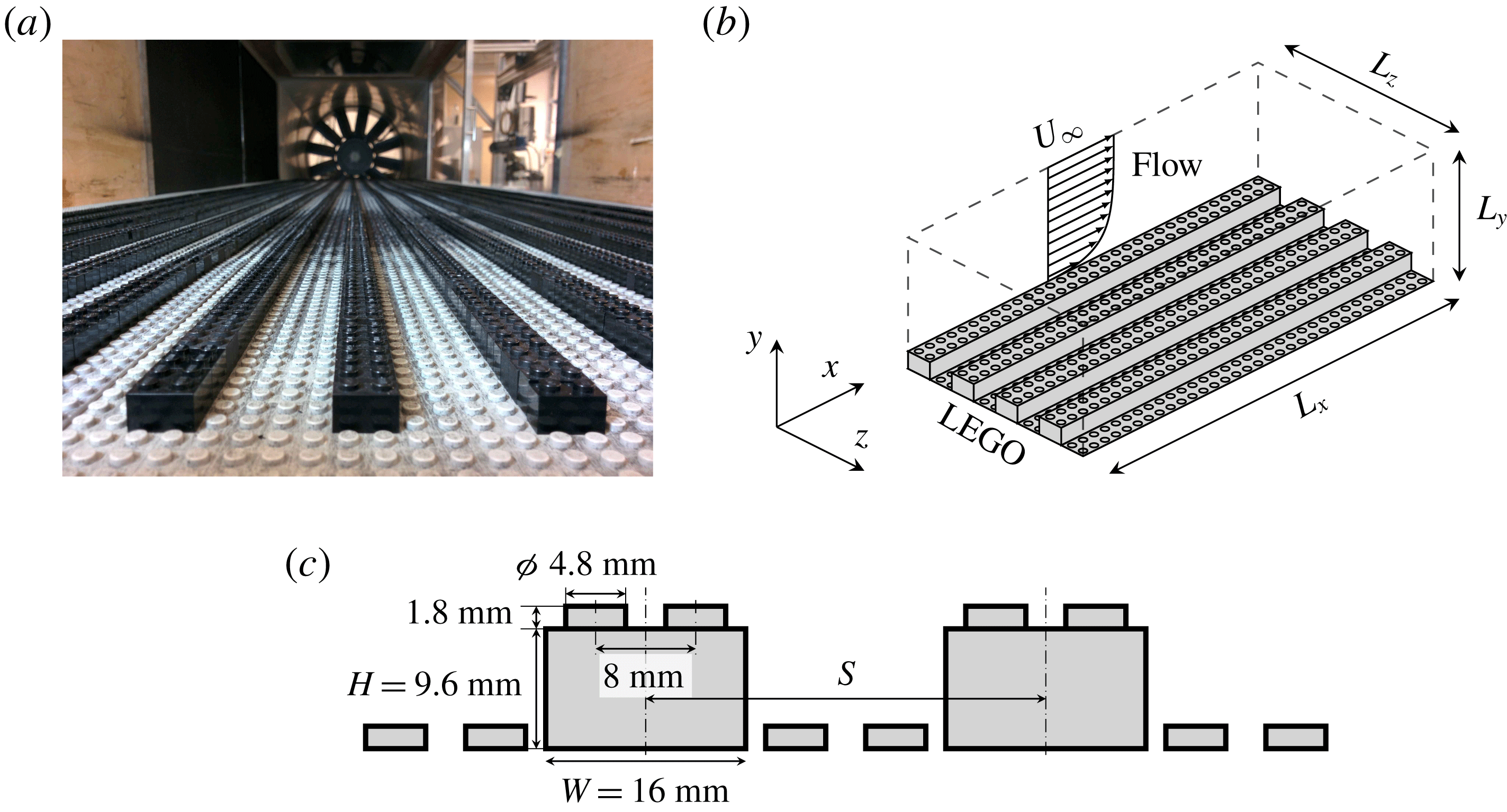
(a) Photograph of the experiment and (b) schematic of the numerical set-up with (c) dimensions of the considered elements and their distribution.

2.1 Experimental set-up
Experiments were performed in the
 $3^{\prime }\times 2^{\prime }$
wind tunnel at the University of Southampton. The test section of the wind tunnel measures
 $0.9~\text{m}\times 0.6~\text{m}\times 4.5~\text{m}$
and has a nominally zero pressure gradient (Castro Reference Castro2007). The rough surface was created with LEGO baseboards and elevated streamwise-aligned strips were created with LEGO bricks (see figure 1
a). The LEGO bricks have a nominal height of
 $H=9.6$
mm, not including the connecting pins which have a height of 1.8 mm (see figure 1
c). In a previous study (Vanderwel & Ganapathisubramani Reference Vanderwel and Ganapathisubramani2015), the centre-to-centre spacing,
 $S$
, of these ridges was varied systematically and it was found that a spacing of the order of the boundary layer thickness,
 $\unicode[STIX]{x1D6FF}$
, was optimal for producing large secondary flows. In this work, we focus on this optimal case where
 $S/\unicode[STIX]{x1D6FF}=0.88$
and investigate the instantaeous characteristics of the secondary flows. In all of the experiments, the free-stream velocity was set to
 $U_{\infty }=15~\text{m}~\text{s}^{-1}$
and the 99 % boundary layer thickness was
 $\unicode[STIX]{x1D6FF}=108\pm 1$
mm. Complementary experiments in the same facility over a smooth surface by Medjnoun et al. (Reference Medjnoun, Vanderwel and Ganapathisubramani2018) demonstrate that the boundary layer thickness changes by less than 5 % when
 $Re_{x}$
is doubled, therefore we can be confident that, with the rough LEGO surface, any changes would be even smaller and that any growth in the boundary layer at the sampling section in the present experiment is negligible, thus enabling comparison with the simulations described in the following section.
Typically, the skin-friction velocity
 $u_{\unicode[STIX]{x1D70F}}$
in experiments is determined indirectly from the plateau of the spanwise-averaged turbulent Reynolds stress near the wall as
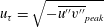 $u_{\unicode[STIX]{x1D70F}}=\sqrt{-\overline{u^{\prime \prime }v^{\prime \prime }}_{peak}}$
(Amir & Castro Reference Amir and Castro2011). However, due to the presence of secondary flows, the dispersive stress contributes a non-negligible amount to the total stress, so a better estimate would be
 $u_{\unicode[STIX]{x1D70F}}=\sqrt{-\overline{u^{\prime \prime }v^{\prime \prime }}_{peak}-\overline{\tilde{u} \tilde{v}}_{peak}}$
, where
 $\tilde{u} \tilde{v}$
represents the dispersive stress component. Neglecting the dispersive stress would, in this case, result in a value of
 $u_{\unicode[STIX]{x1D70F}}=0.63~\text{ms}^{-1}$
, which was the value previously reported by Vanderwel & Ganapathisubramani (Reference Vanderwel and Ganapathisubramani2015); however, including the dispersive contribution produces a revised value of
 $u_{\unicode[STIX]{x1D70F}}=0.74~\text{ms}^{-1}$
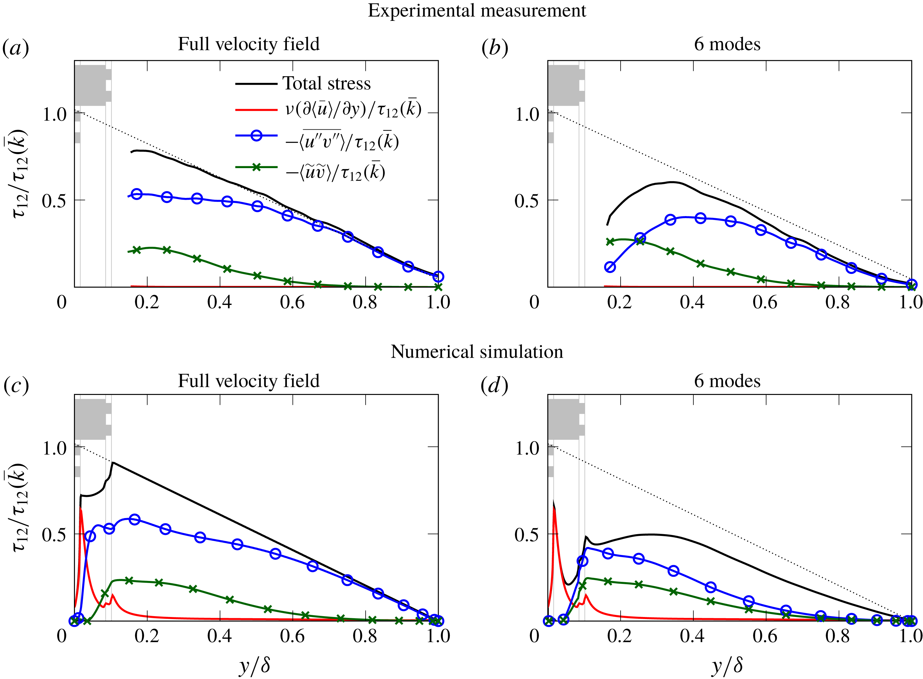
. This approach is confirmed using the DNS data shown later in figure 4, which shows that the dispersive and total stress contribute the majority (81 %) of the total stress at their peak at approximately
 $y/\unicode[STIX]{x1D6FF}=0.15$
; the discrepancy is attributed to the small viscous contribution which would be expected to be even smaller in the experiment than in the DNS. With this value of
 $u_{\unicode[STIX]{x1D70F}}$
, the friction Reynolds number for the experiment is estimated as
 $Re_{\unicode[STIX]{x1D70F}}=u_{\unicode[STIX]{x1D70F}}\unicode[STIX]{x1D6FF}/\unicode[STIX]{x1D708}=4700$
.
Measurements of the flow field that developed over the surface were acquired using stereoscopic particle image velocimetry (PIV). The flow was seeded with vaporized glycol–water solution particles, which were illuminated by a pulsed Nd:YAG laser (Litron 200-15PIV). The measurement plane captured a cross-section of the flow located 4 m downstream from the start of the roughness, where the flow had developed over
 $20\unicode[STIX]{x1D6FF}$
to ensure the fully developed conditions (Castro Reference Castro2007). Particle images were recorded using two LaVision Imager LX 29MP cameras, fitted with lenses having a focal length of 200 mm and an aperture of
 $f$
5.6. The cameras were positioned on one side of the test section on either side of the measurement plane and angled at approximately
 $35^{\circ }$
to the measurement plane. Scheimpflug adapters were fitted to accommodate the oblique viewing angles. For each case, 1500 independent image pairs were acquired at a rate of 2 Hz and converted into vector fields using LaVision’s DaVis 8.2.2 software with a resolution of one vector per 0.9 mm. The uncertainty of the PIV measurements was estimated to be approximately 1 % of
 $U_{\infty }$
. Further details are provided by Vanderwel & Ganapathisubramani (Reference Vanderwel and Ganapathisubramani2015).
2.2 Numerical procedure
The DNS is based on a pseudo-spectral solver for incompressible boundary layer flows (Chevalier et al.
Reference Chevalier, Schlatter, Lundbladh and Henningson2007). The Navier–Stokes equations are numerically integrated using the velocity–vorticity formulation by a spectral method with Fourier decomposition in the horizontal directions and Chebyshev discretization in the wall-normal direction. For temporal advancement, the convection and viscous terms are discretized using the third-order Runge–Kutta and Crank–Nicolson methods, respectively. Figure 1(b) presents the configuration of the numerical experiment with the surface protrusions placed at the lower domain wall and introduces a coordinate system with
 $x=x_{1}$
,
 $y=x_{2}$
and
 $z=x_{3}$
representing streamwise, wall-normal and spanwise coordinate axes, respectively. The corresponding velocity components are denoted by
 $u=u_{1}$
,
 $v=u_{2}$
and
 $w=u_{3}$
, respectively. The simulation domain represents an open turbulent channel flow for which periodic boundary conditions are applied in streamwise and spanwise directions, while the wall-normal extension of the domain is bounded by no-slip boundary conditions at the lower domain wall (
 $y=0$
) and symmetry boundary conditions (
 $v=0$
,
 $\unicode[STIX]{x2202}u/\unicode[STIX]{x2202}y=\unicode[STIX]{x2202}w/\unicode[STIX]{x2202}y=0$
) at the upper boundary (
 $y=\unicode[STIX]{x1D6FF}$
). Domain size and resolution information is summarized in table 1. The domain size is chosen based on the report by Lozano-Durán & Jiménez (Reference Lozano-Durán and Jiménez2014) to ensure appropriate representation of the turbulent scales and hence validity of first- and second-order one-point statistics. Additionally, we carried out a mesh independence study, which confirms the sufficiency of the chosen domain resolution.
The surface structure is introduced through an immersed boundary method (IBM) as discussed in Forooghi et al. (Reference Forooghi, Stroh, Magagnato, Jakirlić and Frohnapfel2017, Reference Forooghi, Stroh, Schlatter and Frohnapfel2018). The method is based on the IBM proposed by Goldstein, Handler & Sirovich (Reference Goldstein, Handler and Sirovich1993) and is essentially a proportional controller which imposes zero velocity in the solid region of the numerical domain. The LEGO structures are placed on the lower domain wall in such a way that the surface height
 $H$
of the large raised surface elements is given by
 $H/\unicode[STIX]{x1D6FF}=8.6\,\%$
which corresponds to the experimental set-up. As in Forooghi et al. (Reference Forooghi, Stroh, Magagnato, Jakirlić and Frohnapfel2017, Reference Forooghi, Stroh, Schlatter and Frohnapfel2018) the flow is driven by a prescribed constant pressure gradient (CPG) which results in a bulk Reynolds number of
 $Re_{b}=U\unicode[STIX]{x1D6FF}/\unicode[STIX]{x1D708}=7161$
. The corresponding effective wall shear stress
 $\unicode[STIX]{x1D70F}_{w}^{\ast }$
is computed by extrapolating the total shear stress from the outer region to the region of the virtual wall location
 $\bar{k}$
, which is given by the mean surface height in the present case (Chan-Braun, García-Villalba & Uhlmann Reference Chan-Braun, García-Villalba and Uhlmann2011; Forooghi et al.
Reference Forooghi, Stroh, Schlatter and Frohnapfel2018). The resulting friction Reynolds number for the present case is given by
 $Re_{\unicode[STIX]{x1D70F}}=\sqrt{\unicode[STIX]{x1D70F}_{w}^{\ast }}\unicode[STIX]{x1D70C}(\unicode[STIX]{x1D6FF}-\bar{k})/\unicode[STIX]{x1D708}=495$
. Therefore, the size of the LEGO elements in viscous units is
 $H^{+}\approx 50$
.
In this paper two statistical data sets are considered: for the two-dimensional distributions in the
 $y$
–
 $z$
-plane the data set based on the runtime simulation statistics with temporal and streamwise averaging is used, while the proper orthogonal decomposition and vortex detection algorithm is applied to a set of 750 temporally uncorrelated three-dimensional fields saved during the simulation run. The runtime statistical integration is performed during a time period of at least 200
 $\unicode[STIX]{x1D6FF}/u_{\unicode[STIX]{x1D70F}}$
after the flow reached fully developed state. This integration time corresponds to 29 000 viscous time units
 $t^{+}=\unicode[STIX]{x1D708}\unicode[STIX]{x1D70C}/\unicode[STIX]{x1D70F}_{w}^{\ast }$
.
Domain configuration with reference values for LEGO surface with
 $S/\unicode[STIX]{x1D6FF}=1$
.

2.3 Key differences in the experiment and simulation
While we strove to make the experiments and numerical simulations comparable, we also acknowledge several key differences that were chosen in order to take advantage of both methodologies. One of the main hypotheses that stemmed from the experimental study was that secondary flows would be maximized when the spacing,
 $S$
, of the features was proportional to the boundary layer thickness,
 $\unicode[STIX]{x1D6FF}$
. Therefore, when designing the simulations, we chose a spacing such that
 $S/\unicode[STIX]{x1D6FF}=1$
; however, we did not have the resources to repeat the experiments with this spacing. As previous work suggests that the presence of secondary flows is fairly robust and that similar flows appear for a range of
 $0.88<S/\unicode[STIX]{x1D6FF}<1.12$
(Vanderwel & Ganapathisubramani Reference Vanderwel and Ganapathisubramani2015), we are confident that any
 $S/\unicode[STIX]{x1D6FF}$
is this range would produce similar secondary flows.
Another key difference is the Reynolds number: in the experiments
 $Re_{\unicode[STIX]{x1D70F}}=4000$
, whereas in the simulations
 $Re_{\unicode[STIX]{x1D70F}}=500$
. As a consequence, the dimensionless height of the LEGO elements in viscous units differs almost by an order of magnitude. If we were to equate these values with the roughness Reynolds number of a classical (i.e. statistically homogeneous) rough surface it would indicate that one of the flows (the experiment) represents a flow in the fully rough regime while the other (the DNS) is more likely to be in the transitionally rough regime. However, the present surface geometry strongly differs from a statistically rough surface. To our knowledge, there is no indication as to whether these flows with large-scale heterogeneities in the spanwise direction and basically homogeneous structures in the streamwise direction actually reach a fully rough state, which is characterized by the fact that form drag is the dominant mechanism of the generated momentum deficit while viscous drag is negligible. What we will find is that, even at the lower Reynolds number, the secondary flows are incredibly robust and behave similarly to those in the experiment at higher Reynolds number. This is in agreement with the findings of Stroh et al. (Reference Stroh, Hasegawa, Kriegseis and Frohnapfel2016), where it is shown that outer scaling is more relevant for the formation of secondary motion than scaling in viscous units.
It is also worth considering that the periodic boundary conditions enforced in the simulation are not exactly the same as the developing boundary layer in the wind tunnel, however, as secondary flows occur in fully turbulent conditions they should not depend heavily on the conditions far upstream. In the following sections, after demonstrating that the experimental and numerical flows are indeed comparable, we make use of these benefits to thoroughly investigate the instantaneous nature of these secondary flows.
3 Results
3.1 Time-averaged secondary flows
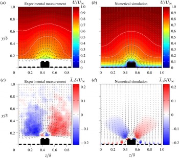
Secondary flows are large regions of recirculation within the boundary layer that appear as large vortical structures in the time-averaged flow fields. These structures are clearly visible in the time-averaged velocity fields in both the experimental measurements and numerical simulations presented in figure 2. The plots show colour contours of the streamwise velocity with velocity vectors representing the in-plane velocity components over one period of the surface pattern. The mean streamwise velocity exhibits large spanwise variations that extend the full thickness of the boundary layer but are most pronounced near the wall. Low-momentum pathways (LMPs) form around the elevated ridges of the surfaces and high-momentum pathways (HMPs) occur in the valleys. Between these zones, large secondary flows form. In both the experiments and the numerical simulations, these vortices extend well beyond the roughness sublayer to approximately
 $0.5\unicode[STIX]{x1D6FF}$
.
Time-averaged velocity and signed swirling strength.

Despite the fact that the numerical simulations correspond to a Reynolds number approximately ten times weaker than the experiments, we find a very similar flow topology, demonstrating the robustness of the secondary flows. This is different from the mean secondary flow in ducts, whose shape changes as a function of Reynolds number (Kawahara et al. Reference Kawahara, Uhlmann and Van Veen2012).
The mean signed swirling strength maps exhibit the secondary flows very clearly and are also presented in figure 2. These maps are computed as the time average of the instantaneous swirling strength multiplied by the sign of the local instantaneous vorticity. The map from the experimental measurements was shown previously by Vanderwel & Ganapathisubramani (Reference Vanderwel and Ganapathisubramani2015) where the large pair of counter-rotating vortices are the secondary flows and the smaller pair of vortices located just above each protrusion were labelled as ‘primary’ flows. When the spacing of the ridges was small, the primary flows dominated and secondary flows did not appear, but as the spacing became
 $O(\unicode[STIX]{x1D6FF})$
the secondary flows manifested. The map from the numerical simulations produces the same vortex topology. The magnitude of the swirling strength is the same order of magnitude as those in the experiment.
The map from the numerical simulations now provides access to what is happening below the roughness height. It illustrates how the ‘primary’ vortices emanate from the corners of the large surface protrusions, and that the secondary vortices appear detached and engulf the bulk of the boundary layer. Smaller vortex pairs are also produced by each of the small bumps in the valleys; however, proximity to the larger secondary flows mitigates the strength of one side of this smaller vortex pair for many of the bumps. Notice that in the middle of the valley (
 $z/\unicode[STIX]{x1D6FF}=0,1$
) both sides of this small vortex pair appear with nearly equal strength over the roughness bumps. The vortices associated with the small roughness bumps are not expected to influence the secondary flows significantly. To test this, the numerical simulations were repeated with all the connecting pins of the LEGO removed. These results are shown in the Appendix and demonstrate that the same structure of primary and secondary flows persists around a square wall protrusion.
3.2 Instantaneous velocity fields
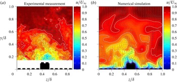
It is clear that secondary flows are a dominant feature of the time-averaged flow fields, however, what is still unclear is how these secondary flows feature in the instantaneous snapshots of the flow. Example snapshots (taken from the supplementary movies) of the instantaneous velocity field are presented in figure 3. It is immediately apparent that the structure of the instantaneous flow is completely different and more complex than the time-averaged flow field. The vector fields of the in-plane motion do not exhibit large zones of recirculation but rather much finer-scale motions consistent with the scale of the wrinkles in the interfaces of the low- and high-momentum pathways. The bases of the low-speed zones remain fixed above the elevated regions of the surface; however, the low-momentum pathways themselves extend far away from the wall in narrow wisps that wave from side to side in the flow in a way that brings to mind the motion of a candle flame. Similarly, high-momentum pathways penetrate the boundary layer and reach close to the wall in the regions above the valleys of the surface roughness.
Snapshots of the instantaneous flow field from the experiment and the simulation (videos of the experimental measurements and the simulation results are available online in mp4 format on the Cambridge Core website, please see supplementary movies available at https://doi.org/10.1017/jfm.2018.955).

In the following sections we apply several analyses to the instantaneous snapshots in order to better understand the structure of the instantaneous flow features. We investigate how the presence of the secondary motions is reflected in dispersive and random contributions to the Reynolds stresses and which of the discrete structures present in the instantaneous maps are relevant to make up the large secondary flows that are observed in the time-averaged flow fields.
3.3 Reynolds stress distribution
The spanwise inhomogeneity of the Reynolds stresses is known to sustain secondary motions of Prandtl’s second kind. Based on the mean momentum budget or streamwise vorticity transport one can identify particular gradients of the Reynolds stress tensor compensating for the presence of the secondary motion (Anderson et al. Reference Anderson, Barros, Christensen and Awasthi2015; Dai et al. Reference Dai, Huang, Xu and Cui2015; Stroh et al. Reference Stroh, Hasegawa, Kriegseis and Frohnapfel2016). Due to the periodically varying surface inhomogeneity in the spanwise direction we expect a similar periodicity in the statistical features of the flow field. A measure for the additional momentum transport due to surface inhomogeneities in rough-wall boundary layers is given by the so-called dispersive stresses (Finnigan Reference Finnigan2000; Cheng & Castro Reference Cheng and Castro2002; Finnigan & Shaw Reference Finnigan and Shaw2008). The definition of dispersive stresses is based on a distinction between spatial and temporal averaging in the definition of the velocity fluctuations.
In the present set-up, a triple decomposition, as suggested by Reynolds & Hussain (Reference Reynolds and Hussain1972), can be employed. The triple decomposition of the velocity component
 $u_{i}$
in the
 $y$
–
 $z$
cross-plane is given by
 $$\begin{eqnarray}u_{i}(y,z,t)=\langle \bar{u}_{i}\rangle (y)+\tilde{u} _{i}(y,z)+u_{i}^{\prime \prime }(y,z,t),\end{eqnarray}$$
where
 $\langle \bar{u}_{i}\rangle$
is the time-averaged and spanwise-averaged field,
 $\tilde{u} _{i}$
and
 $u_{i}^{\prime \prime }$
denote dispersive and random fluctuations, respectively. Combination of the second and third terms from (3.1) gives the total fluctuation
 $$\begin{eqnarray}u_{i}^{\prime }(y,z,t)=\tilde{u} _{i}(y,z)+u_{i}^{\prime \prime }(y,z,t).\end{eqnarray}$$
This approach is explained in detail in Türk et al. (Reference Türk, Daschiel, Stroh, Hasegawa and Frohnapfel2014). With this framework, the spatially averaged stress tensor becomes
 $$\begin{eqnarray}\unicode[STIX]{x1D70F}_{ij}=\underbrace{\unicode[STIX]{x1D708}\frac{\unicode[STIX]{x2202}\langle \bar{u}_{i}\rangle }{\unicode[STIX]{x2202}x_{j}}}_{viscous\,stress}\underbrace{-\langle \overline{u_{i}^{\prime \prime }u_{j}^{\prime \prime }}\rangle }_{\,random\,stress}\,\,\underbrace{-\langle \tilde{u} _{i}\tilde{u} _{j}\rangle }_{dispersive\,stress}.\end{eqnarray}$$
In addition to the usual viscous stress and Reynolds random stress,
 $\unicode[STIX]{x1D70F}_{ij}$
also contains the dispersive stress
 $\langle \tilde{u} _{i}\tilde{u} _{j}\rangle$
, which represents the transport of momentum due to the spanwise heterogeneity of the mean flow. The dispersive stresses are a measure of the spatial inhomogeneity of the flow, as a time-averaged turbulent flow field without any spanwise variations would exhibit zero dispersive stresses.
Viscous, random and dispersive components of the total shear stress
 $\unicode[STIX]{x1D70F}_{12}=\unicode[STIX]{x1D708}(\unicode[STIX]{x2202}\langle \bar{u}\rangle /\unicode[STIX]{x2202}y)-\langle \overline{u^{\prime \prime }v^{\prime \prime }}\rangle -\langle \tilde{u} \tilde{v}\rangle$
evaluated from the experimental measurement (a,c) runtime statistics of the numerical simulation. Corresponding statistical quantities computed from the velocity fields reconstructed with 6 POD modes are shows in (b,d).

Figure 4 demonstrates the contributions of the viscous, random and dispersive stresses to the total shear stress
 $\unicode[STIX]{x1D70F}_{12}$
in the experiment (a,b) and the numerical simulation (c,d). The profiles are normalized by the total shear stress extrapolated to the location of average surface height
 $\bar{k}=0.017\unicode[STIX]{x1D6FF}$
(in the experiment) and
 $\bar{k}=0.019\unicode[STIX]{x1D6FF}$
(in the DNS). Note, that the POD-filtered results as shown in figure 4(b,d) will be discussed in § 3.4, but appear next to figure 4(a,c) for optimal comparability.
The relative contributions of dispersive stress and turbulent stress to the total stress are very similar in both cases, which demonstrates that both the experiment and simulation generate very similar secondary flows. We find a much smaller contribution of the viscous stress to the total stress in the experiment; however, this difference is related to the difference in Reynolds number. At the larger experimental Reynolds number the region where the viscous stress prevails would have been much smaller and is not captured here.
It is evident that the dispersive stress is not only present in the vicinity of the surface roughness but also strongly augments the random stress in the region
 $0.1<y/\unicode[STIX]{x1D6FF}<0.7$
, where it constitutes up to
 $28\,\%$
of the total stress for numerical and experimental data. These findings differ from turbulent flows over irregular rough surfaces where large secondary motions do not occur. For irregular rough surfaces the dispersive stress is restricted to the vicinity of the rough surface and its maximum contribution to the total shear stress is significantly weaker, e.g. approximately
 $16\,\%$
–
 $17\,\%$
as reported by De Marchis, Napoli & Armenio (Reference De Marchis, Napoli and Armenio2010) or Forooghi et al. (Reference Forooghi, Stroh, Schlatter and Frohnapfel2018). Also for regular roughness structures without secondary motions, the reported dispersive stresses are significantly smaller (Coceal et al.
Reference Coceal, Thomas, Castro and Belcher2006; Xie & Fuka Reference Xie and Fuka2018). The present results confirm the observation reported by Vermaas, Uijttewaal & Hoitink (Reference Vermaas, Uijttewaal and Hoitink2011) that the momentum exchange due to secondary flow can be the same order of magnitude as turbulent momentum exchange.
Distribution of dispersive fluctuations
 $\widetilde{u_{i}}$
and their products
 $\widetilde{u_{i}}\widetilde{u_{j}}$
for experimental measurement and numerical simulation.

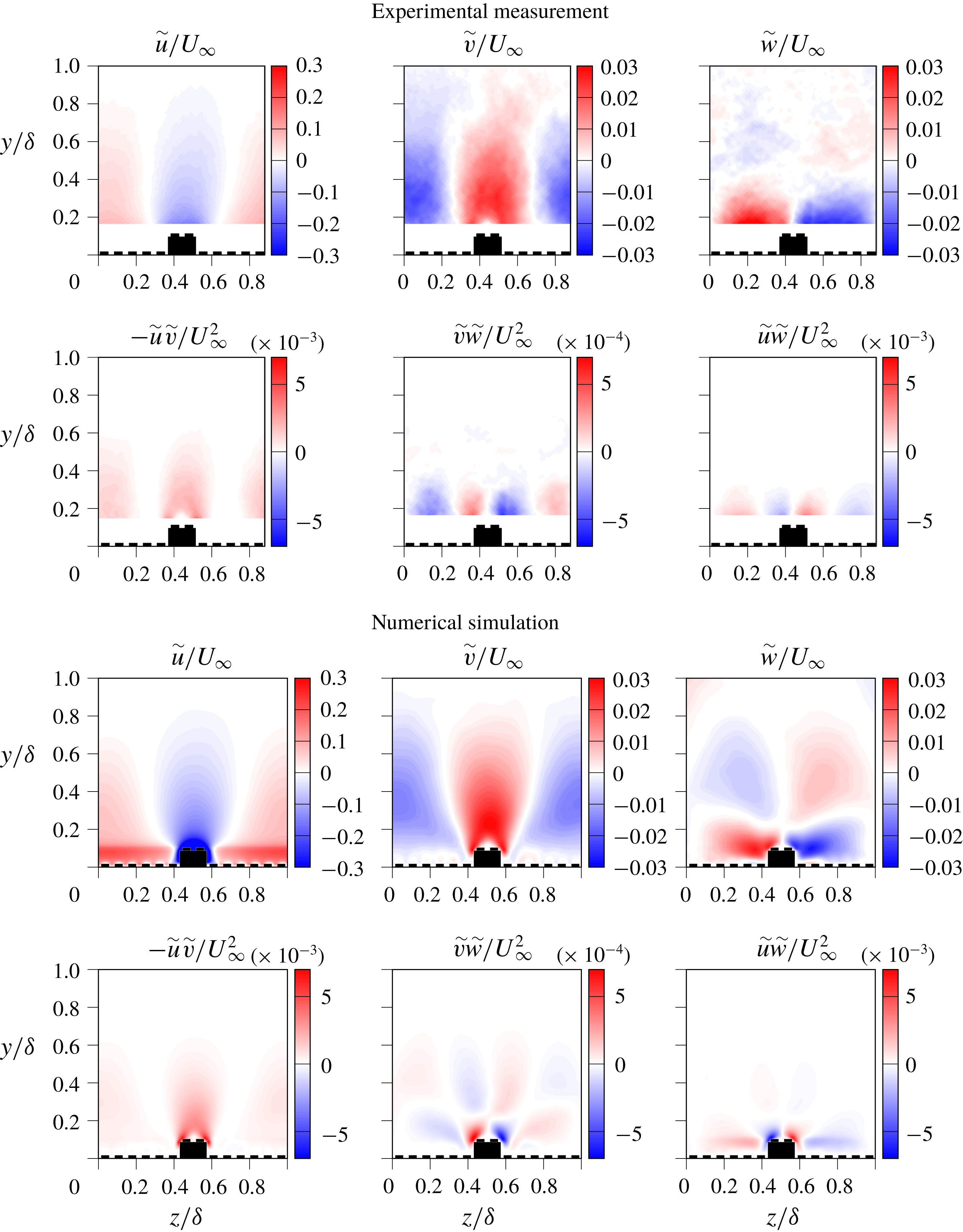
In order to visualize the origin of the dispersive stresses, maps of the dispersive fluctuations and their products are presented in figure 5. The fluctuating components
 $\tilde{v}$
and
 $\tilde{w}$
directly correspond to the time-averaged secondary motion indicated by the arrows in figure 3, while
 $\tilde{u}$
is related to the bulging of the mean streamwise velocity profile visible in the same figure. The spatially averaged covariance of the dispersive fluctuations gives the dispersive stresses from (3.1). The comparison between experimental and numerical data reveals good qualitative and quantitative agreement. The only visible difference is in the wall-normal location at which
 $\tilde{w}$
changes its sign. This is located around
 $y/\unicode[STIX]{x1D6FF}=0.4$
for the experiment whereas it is found below
 $y/\unicode[STIX]{x1D6FF}=0.3$
in the simulation data. From the DNS results it can be seen that the near-wall region in between the raised surface elements does not contribute substantially to the dispersive stress, which suggests that the large-scale secondary flows are the main source of the observed large contribution of the dispersive stress
 $-\langle \tilde{u} \tilde{v}\rangle$
to the total shear stress. The secondary flow basically generates large-scale regions with up-drafts of low-speed momentum and downwashes of high-speed momentum occurring above the peaks and valleys of the surface, respectively.
Time-averaged products of random fluctuations for experimental measurement and numerical simulation.

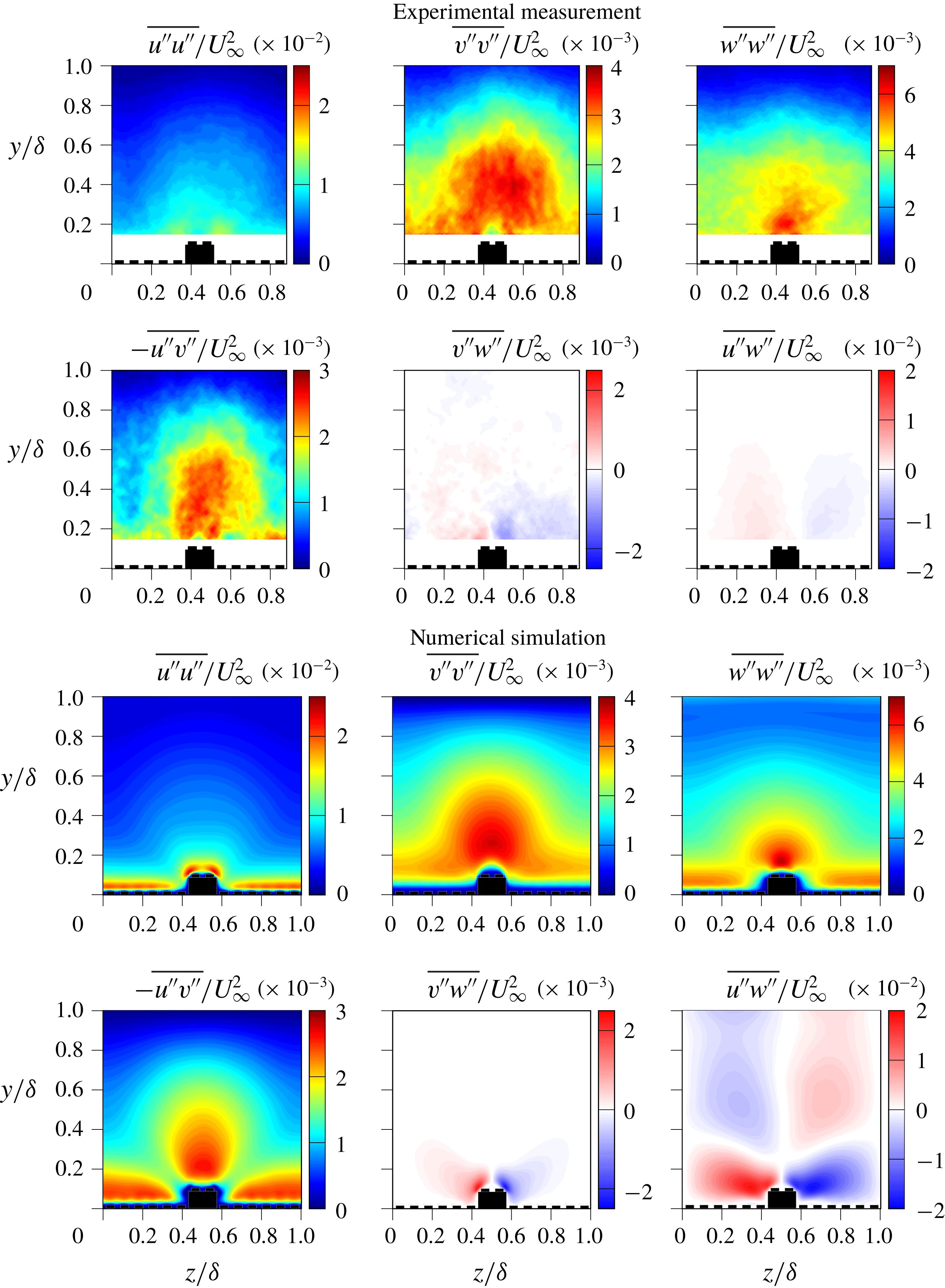
Figure 6 shows the spatial distributions of the random stresses. For these data, we also see very good agreement between experimental and numerical results. Note that due to the nature of the applied averaging, the top row of figure 6 represents
 $\overline{u_{i}^{\prime \prime }u_{i}^{\prime \prime }}$
whereas the top row of figure 5 contains
 $\widetilde{u_{i}}$
. By definition
 $\overline{u_{i}^{\prime \prime }u_{i}^{\prime \prime }}$
can only assume positive values.
It can be seen that
 $\overline{v^{\prime \prime }v^{\prime \prime }}$
, and to a lesser extent also
 $\overline{w^{\prime \prime }w^{\prime \prime }}$
, is mainly concentrated in a large blob around the elevated region of the surface. This suggests that the up-draft of the secondary motion is accompanied by strong random fluctuations while the region of downwash appears to be much calmer. Hence, the secondary flow does not only generate significant dispersive stress, but also appears to reorganize the turbulent stress such that higher turbulence intensity is found above the elevated ridges. This will be further investigated in § 3.6.
With respect to the contributions to the total stress to
 $\unicode[STIX]{x1D70F}_{12}$
, it can be observed that in the outer flow region (
 $y>0.15\unicode[STIX]{x1D6FF}$
),
 $-\langle \overline{u^{\prime \prime }v^{\prime \prime }}\rangle$
is strongly governed by the enhanced wall-normal fluctuations above the elevated ridges, while the contribution in the near-wall region in between the elements seems to stem from the classical near-wall turbulence behaviour. In contrast, the main contribution to
 $-\langle \tilde{u} _{i}\tilde{u} _{j}\rangle$
is located just above the edges of the elevated ridges where strong upward motions occur simultaneously with low streamwise velocities. It is also worth noting the scales of each of these maps which again demonstrate that the random stresses are comparable in magnitude to that of the dispersive stresses.
3.4 Proper orthogonal decomposition
In order to identify the highest energy-containing flow structures and to gain insight into the impact of large-scale flow patterns on the overall secondary flows, the sets of instantaneous flow fields were decomposed with POD using snapshot POD as introduced by Sirovich (Reference Sirovich1987). Accordingly, the convolution of eigenvectors and underlying velocity basis, in contrast to the direct POD, provides the spatial velocity patterns, i.e. the POD modes. A straightforward implementation is described by Meyer, Pedersen & Özcan (Reference Meyer, Pedersen and Özcan2007), for instance.
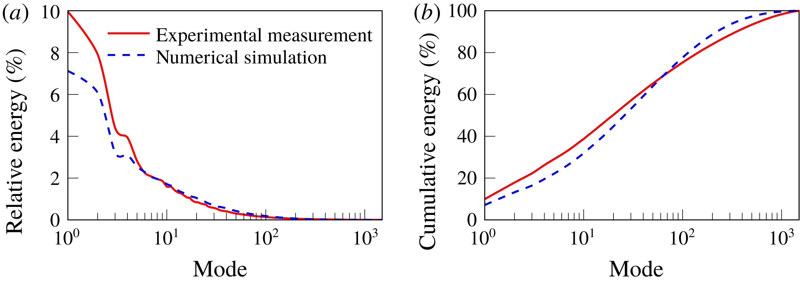
The relative and cumulative energy distributions of the POD modes are presented in figure 7, which shows that roughly
 $20$
modes are required to capture
 $50\,\%$
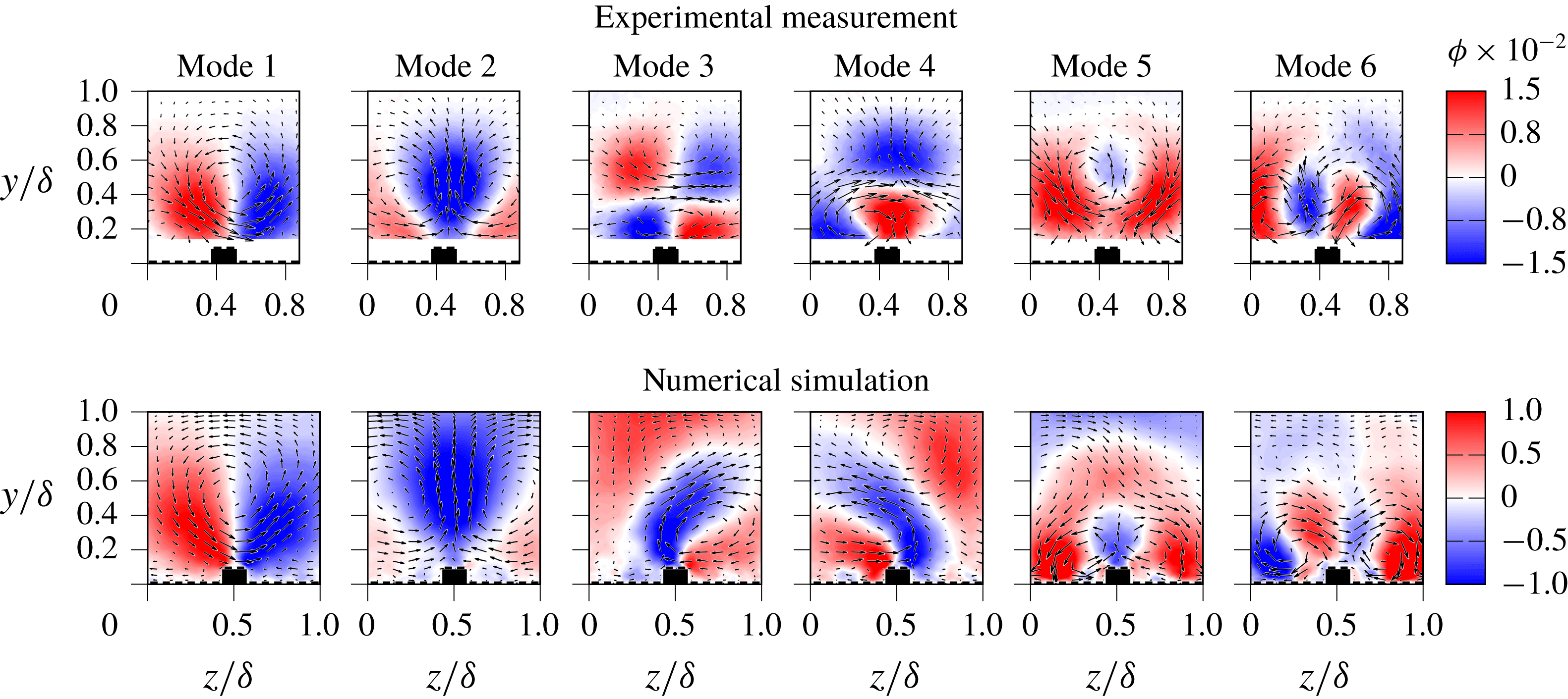
of the turbulent kinetic energy of the flow. However, investigation of the corresponding flow patterns indicates that the first six modes are associated with large-scale (
 $\unicode[STIX]{x1D6FF}$
-scale) motion. Therefore, a basis of these six characteristic patterns has been chosen to test the hypothesis that this class of patterns predominates the secondary motions.
The relative and cumulative energy distributions across the modes.

These first six modes are presented in figure 8 for both the numerical and experimental data. In both cases, the data are cropped to a single period of the surface pattern. Both the experiment and the simulations reveal nearly identical flow patterns in these first few modes. The dominant modes (modes 1 and 2) are large vortical motions that fill the boundary layer depth and are essentially lateral shifts of the main secondary flow patterns. The later modes (3–6) divide the flow up into smaller vortices but still are quite active right out to the edge of the boundary layer. As the mode number increases further, the size of the vortices decreases, and the range of vortex scales corresponds with the cascade of scales in turbulence.
The reduced basis of six modes captures roughly one third of the turbulent kinetic energy (see figure 7). Interestingly, a reconstruction of the instantaneous snapshots using only the first six modes provides
 $66\,\%$
of the total magnitude of the total Reynolds stress
 $\overline{u^{\prime }v^{\prime }}$
, illustrating that these large-scale features are responsible for the majority of the Reynolds stress. We note that the dispersive contribution to the Reynolds shear stress is determined by the spanwise variation of the mean flow field, therefore it is not surprising that the POD-based model captures a large percentage of
 $\overline{u^{\prime }v^{\prime }}$
. The suitability of the reduced basis of models is further emphasized in figure 4, where the direct comparison of full and filtered data sets demonstrates that the dispersive stresses are preserved with the six-mode basis.
The fact that the simulations and the experiments produce similar modes despite the fact that the experimental data are missing at the wall indicates that the near-wall motions are not very important – at least in terms of energy contribution. Repeating the analysis using a wider domain confirmed that the largest structures are centred on the raised ridges of the surface, as shown in modes 1 and 2. The fact that they do not exceed the dimensions of the single period domain retroactively verified the choice of this particular domain, which consequently was used for all subsequent analyses.
Even though the shape of the energy distributions of the POD modes are consistent between the experiment and the simulation, there is a slight variation in the magnitudes of the lower modes, as can be identified from figure 7. This can be attributed to the different spatial resolution of the data as it is well established that a coarsely resolved data set will lead to a larger fraction of energy in lower modes (Placidi & Ganapathisubramani Reference Placidi and Ganapathisubramani2018) and the resolution of the present experiments is more coarse than the DNS.
The highest energy modes present in the flow over the roughness.

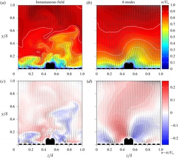
Complete instantaneous flow field with its POD-reconstructed counterpart (a,b) and the corresponding velocity fluctuations (c,d). In the upper row, the colour code corresponds to the streamwise velocity component and the arrows indicate the in-plane motion, whereas in the bottom row, the colour code represents the instantaneous deviation of the streamwise velocity component from
 $\langle \bar{u}\rangle (y)$
. A video of the temporal flow evolution based on the DNS data and the reduced-order reconstruction is available online in mp4 format on the Cambridge Core website.

While the POD modes do not represent actual realizations of the flow, they do indicate how the energy in the velocity fluctuations is distributed. For the present case, it has been shown that the highest energy flow patterns correspond to large
 $\unicode[STIX]{x1D6FF}$
-scale vortical motions. The fact that the dominant features of the secondary motions are captured by the six most energetic modes in turn means that it is possible to use a POD filter to focus the analysis of the instantaneous data on the large-scale motions. In the following sections, we use the results of the POD to reconstruct ‘filtered’ instantaneous velocity fields using the reduced basis of six modes. A snapshot of the reconstructed flow field in comparison to the full DNS velocity field is shown in figure 9. The lateral shift related to the first two modes of figure 8 is clearly visible in the corresponding movie. This large-scale lateral motion appears to be a characteristic dynamic behaviour of the secondary motion which is consistently observed in experiments and DNS.
In general, it can clearly be observed that the reduced-order reconstruction removes the effects of the finer fluctuations (which have relatively less energy) and maintains only the large-scale motions (which contribute the majority of the total Reynolds stress
 $\overline{u^{\prime }v^{\prime }}$
). In the following we use the ‘filtered’ flow field in comparison with the full flow field in order to analyse whether characteristic instantaneous features of the secondary flow can be captured with the most energetic modes only.
3.5 Vortex identification
The time-averaged results in § 3.1 show that the time-averaged secondary flow consists of a large counter-rotating vortex pair, with many smaller vortices located near the wall. However, we would like to identify if the instantaneous fields also contain such large counter-rotating vortical structures or if they are simply the result of a inhomogeneous distribution of smaller structures. If the latter, what then are the characteristics of the instantaneous vortices and their distribution?
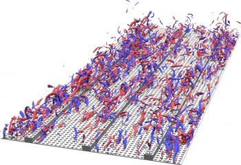
Instantaneous structure of the flow visualized using isosurfaces of
 $\unicode[STIX]{x1D706}_{2}$
-criterion (
 $\unicode[STIX]{x1D706}_{2}=-0.005$
) and coloured by their rotational direction (video of the simulation visualization is available online in mp4 format on the Cambridge Core website).

Figure 10 (and the associated movie) show the instantaneous three-dimensional flow structure from the DNS. This looks qualitatively similar to what one would expect to see when visualizing a smooth turbulent boundary layer (e.g. Wu & Moin Reference Wu and Moin2009); however, in the present case, the flow structures seem to predominantly appear in the regions along the ridges, which is in agreement with the observed enhanced turbulence intensity in the region above the ridges. Similar observations in visualizations of the near-wall turbulent structures have been previously reported in flows with spanwise heterogeneity of boundary conditions resulting in formation of secondary flows (Benschop & Breugem Reference Benschop and Breugem2017; Ni et al.
Reference Ni, Lu, Fang, Moulinec and Yao2018) or flows with directly induced large-scale secondary motion (Canton et al.
Reference Canton, Örlü, Chin, Hutchins, Monty and Schlatter2016). Additionally, one can also observe a local clustering of the detected structures mainly located along the sides of the ridges. These small-scale vortex groups are rather compact, exhibiting a streamwise extent of approximately
 $2{-}3\unicode[STIX]{x1D6FF}$
and appear to be convected downstream along the ridges, slowly changing their composition and shape.
In order to further characterize the vortices we applied a vortex identification algorithm to identify the vortices in the instantaneous snapshots from the experiments and the simulations. The algorithm used peaks in swirling strength above a fixed threshold to identify the locations of vortices and then applied an area-growing algorithm to determine the extent of each of the vortices (Vanderwel & Tavoularis Reference Vanderwel and Tavoularis2011). The circulation of each vortex was then determined by integrating the vorticity over the area of the vortex. The swirling strength maps were determined for the full flow field and for the reduced-order instantaneous velocity maps reconstructed from six POD modes as outlined in the previous section.
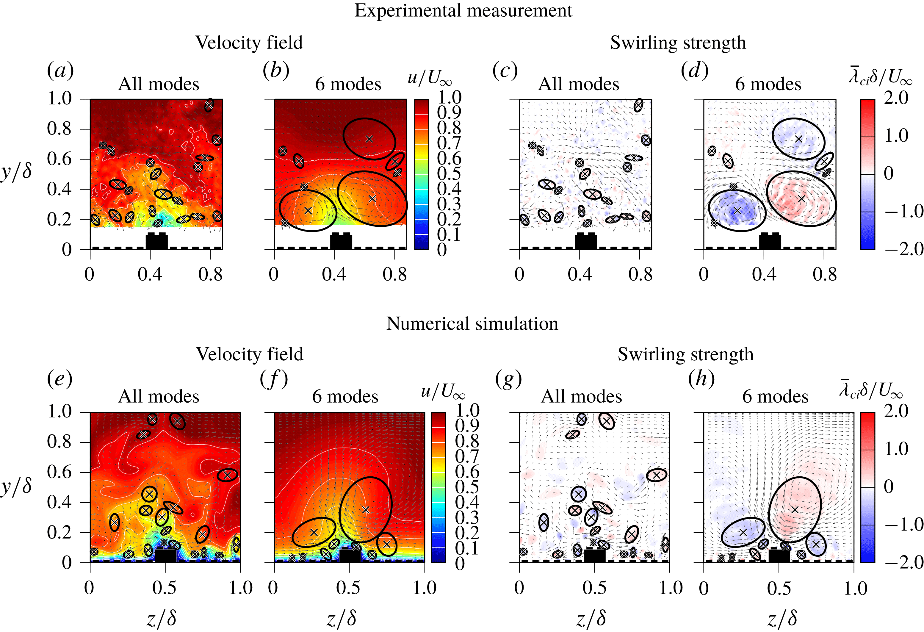
Flow diagram showing an example of using a reduced-order model to effectively filter the instantaneous snapshots while preserving the highest energy structures. (a,e) The original instantaneous velocity map. (b,f) The reconstructed map using only 6 modes. (c,d,g,h) The vortices identified from peaks in swirling strength.

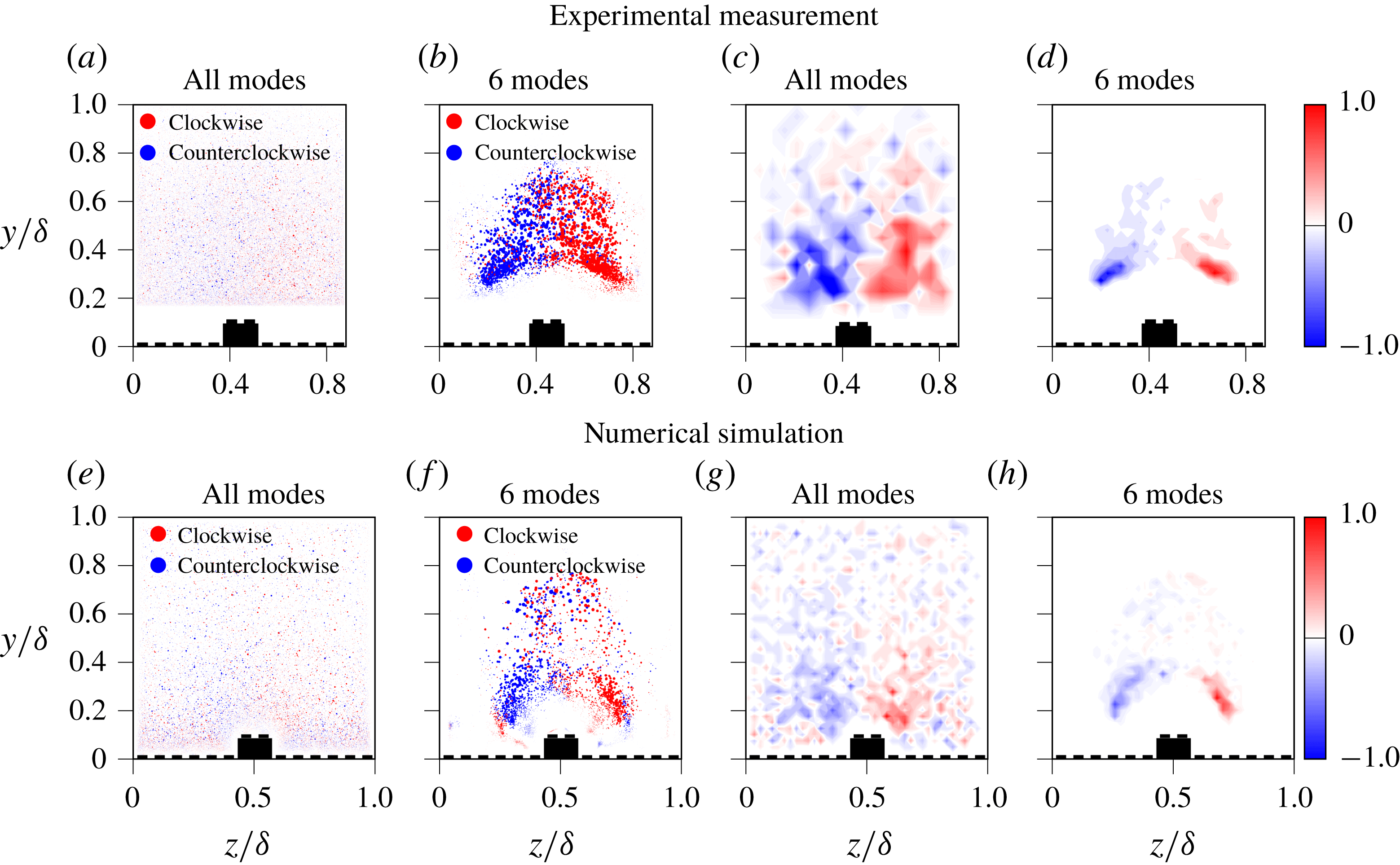
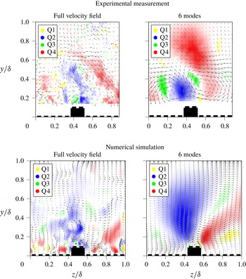
Figure 11 provides an example of the process, where filtered and unfiltered velocity fields and the corresponding swirling strength of random snapshots from both data sets are shown. We found that the typical snapshot has over 100 discrete vortices identified but that only 2–3 of them are dominant, with total circulations two orders of magnitude larger than the rest. Furthermore, in 91 % of instances, the two largest vortices had opposite rotation, indicating the predominance of vortex pairs. However, the average diameter of these dominant vortices is considerably smaller than the time-average secondary vortices, as demonstrated in figure 11(c,g). The swirling strength distributions of the reduced basis emphasize the dominant (counter-rotating) vortices and eliminate the small-scale fluctuations (see figure 11 d,h). The validity of this elimination process is shown in figure 12, where scatter plots summarize all the locations of all the vortices and provide the resulting probability distribution of the locations of the vortices. Interestingly, at first glance, the unfiltered data indicate an even distribution of vortex locations across the domain (figure 12 a,e). The corresponding probability density functions (PDF) as plotted in figure 12(c,g), however, indicate that clockwise vortices tend to occur to the right of the elevated ridge, while counter-clockwise vortices occur to the left, consistent with the pattern of the secondary motions. The filtered data clearly emphasize this trend, since the randomly oriented small-scale fluctuations are eliminated from the scatter plots (figure 12 c,g), which in turn also results in more salient spatial separation of the counter-oriented events (see figure 12 d,h). Here, the immediate comparison of filtered and unfiltered PDFs particularly shows that the six-mode basis is sufficient to capture a major property of the instantaneous flow behaviour.
Overall, this leads us to conclude that, in the instantaneous flow fields, the secondary flows manifest as smaller yet stronger counter-rotating vortex pairs, that can appear in a range of orientations but average out to form these large secondary flow structures in the mean. These findings are consistent with the results of Kevin et al. (Reference Kevin, Monty, Bai, Pathikonda, Nugroho, Barros, Christensen and Hutchins2017), who investigated how the secondary flow patterns are organized in instantaneous snapshots of the flow over converging–diverging riblets. They also filtered their data and found that the diameters of the instantaneous motions were on average smaller than the time-averaged secondary flows and that the centre of these motions meandered in space. They also concluded that the large
 $\unicode[STIX]{x1D6FF}$
-scale secondary flows were ‘the superposition of stronger individual vortices’.
Scatter plot of vortex locations and difference of PDF distribution between clockwise and counter-clockwise rotating vortices.

3.6 Instantaneous stresses
In a similar way to our analysis of the instantaneous vortex distribution, we can also investigate the instantaneous structure of the Reynolds random stress field. The time-averaged maps of Reynolds random stress
 $\overline{u^{\prime \prime }v^{\prime \prime }}$
shown in figure 6 indicate that a high magnitude of stress is concentrated above the elevated surfaces and extends beyond
 $y/\unicode[STIX]{x1D6FF}=0.5$
. By investigating the instantaneous maps of this quantity, we can assess whether this is the result of the superposition of many smaller ejection/sweep events or whether the instantaneous stress events also extend to most of the depth of the boundary layer.
Instantaneous distribution of the Reynolds random stresses
 $u^{\prime \prime }v^{\prime \prime }$
, coloured by their quadrant based on the original velocity data and on the reduced-order filtered velocity data.

Figure 13 presents typical instantaneous maps of the Reynolds random stress
 $u^{\prime \prime }v^{\prime \prime }$
from both the experiment and the simulations. The unfiltered stress maps are shown alongside maps determined from the reduced-order instantaneous velocity maps reconstructed using six POD modes, in order to focus on the large-scale motions in the flow as was done when analysing the vortices. In this case, the POD filtering is crucial to identify the appropriate extent of the dominant structures, which would otherwise be obscured by the fine-scale turbulence. Events are categorized (and coloured) via quadrant analysis based on the sign of the local vertical and streamwise velocity fluctuations, such that the Q2 events (
 $u^{\prime \prime }<0$
,
 $v^{\prime \prime }>0$
) are associated with ejections and Q4 events (
 $u^{\prime \prime }>0$
,
 $v^{\prime \prime }<0$
) are associated with sweeps, following previous studies which also employed quadrant analysis (Finnigan Reference Finnigan1979; Antonia Reference Antonia1981; Vanderwel & Tavoularis Reference Vanderwel and Tavoularis2016).
We find that the magnitudes of the instantaneous stresses are similar to the magnitudes of the time-averaged Reynolds and dispersive stresses (i.e.
 $u^{\prime \prime }v^{\prime \prime }/U_{\infty }^{2}\sim 4\times 10^{-3}$
). The Q2 and Q4 events are dominant and often appear to alternate along the span with a period similar to the roughness spacing. Between these events the vector maps show the signatures of vortices. The dominant instantaneous Q2 and Q4 events appear to have an average vertical extent of
 $0.4\unicode[STIX]{x1D6FF}$
, indicating that these important momentum transfer events extend over a large portion of the boundary layer thickness.
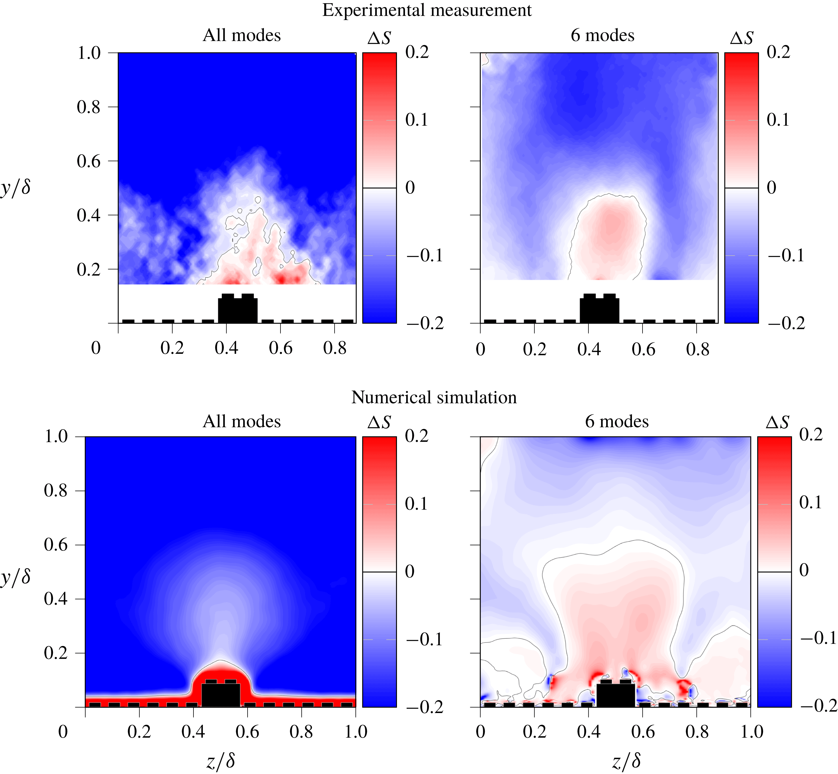
Q4 events (sweeps) appear to occur closer to the surface whereas Q2 events (ejections) appear to occur further away from the surface, which is consistent with the fact that sweeps tend to dominate momentum transfer near the wall for flows over rough surfaces (Raupach Reference Raupach1981). Following Raupach’s analysis, this difference is highlighted by plotting a map of the difference between the fractional stress contributions by sweeps and ejections as
 $$\begin{eqnarray}\unicode[STIX]{x0394}S=S_{4}-S_{2},\quad \text{where }S_{i}=\langle u^{\prime \prime }v^{\prime \prime }\rangle _{i}/\overline{u^{\prime \prime }v^{\prime \prime }}.\end{eqnarray}$$
Maps of
 $\unicode[STIX]{x0394}S$
are presented in figure 14 from the experimental and numerical data, with and without the POD filter. In all the cases,
 $\unicode[STIX]{x0394}S$
becomes positive with values of approximately 0.2–0.9 in the proximity of the elevated surface element, which is only slightly larger than the range of values between 0.1 and 0.5 observed by Raupach in a rough-wall turbulent boundary layer with
 $Re_{\unicode[STIX]{x1D70F}}\sim 400$
. The main difference observed between the present results and those from a rough boundary layer without secondary flows is that
 $\unicode[STIX]{x0394}S$
is not uniform across the span and the region of positive
 $\unicode[STIX]{x0394}S$
(where sweeps dominate) extends much farther into the outer boundary layer, due to the presence of the secondary flows. This extended region of positive
 $\unicode[STIX]{x0394}S$
coincides with the location of upwash in the mean velocity fields; so, although the mean dispersive velocity component is upwards, the dominant fluctuations are downwards sweeps. This makes sense as the largest stresses would occur when the velocity fluctuation is the most different from the mean, and this would be consistent with a lateral instability of the large-scale low-momentum regions, which was observed by Kevin et al. (Reference Kevin, Monty, Bai, Pathikonda, Nugroho, Barros, Christensen and Hutchins2017).
Maps of the fractional difference between the stress contributions by sweeps and ejections,
 $\unicode[STIX]{x0394}S=S_{4}-S_{2}$
for full velocity fields and velocity field reconstructed with 6 POD modes.

It is interesting to see that this extended region of positive
 $\unicode[STIX]{x0394}S$
is least accentuated with the unfiltered DNS results and most accentuated when the six-mode POD reconstruction is applied. This suggests that the scale resolution of the data affects this property of the turbulent flow. The unfiltered DNS is effectively the most finely resolved data set capturing all the fine-scale structures, whereas the experimental data are effectively filtered at the PIV resolution of approximately 35 wall units, and of course the six-mode reconstructions isolate the contributions of the large-scale dominant flow structures. This leads to the conclusion that, away from the wall in the upwash created by the secondary flows, the large-scale motions comprise predominantly sweeps (which lead to positive
 $\unicode[STIX]{x0394}S$
) whereas the smaller-scale motions appear to be mostly ejections (which, when included, tend to decrease
 $\unicode[STIX]{x0394}S$
). In other words, when the data are limited to only the dominant larger-scale structures, the extended region of positive
 $\unicode[STIX]{x0394}S$
is enhanced, highlighting the inhomogeneity of the flow due to secondary flows.
This analysis demonstrates that the Reynolds random stress appears to be the superposition of strong individual stress events, that meander somewhat around the region of the elevated surfaces and often extend far into the outer boundary layer. These stress events appear superimposed on the mean dispersive secondary flow structure and can take the opposite direction of the mean flow. The spatial organization of the turbulent flow structures is attributed to the secondary flows that manifest in these flows, which leads to greater turbulent Reynolds stress in the regions above the elevated surfaces, composed of mainly Q4 events (sweeps) typical of near-wall behaviour in homogeneous rough walls.
4 Conclusions
This work has investigated the instantaneous structure of the secondary flows that can appear over turbulent boundary layers over surfaces with spanwise heterogeneities. Secondary flows manifest as large counter-rotating vortices that engulf a large portion of the boundary layer and have been previously linked to Prandtl’s instabilities of the second kind. We have captured these features in both experimental and numerical simulations, which provide complementary measurements of the properties of these flows. The instantaneous velocity fields that comprise the secondary flows are very complex and differ from the time-averaged picture. Low-momentum pathways appear fixed to the elevated surface regions, but extend deep into the boundary layer in narrow wisps that meander in the turbulent flow.
The distribution of Reynolds stresses was investigated and we find that spatial gradients in Reynolds shear stresses can be related to the presence of the mean secondary flow, consistent with the findings of Anderson et al. (Reference Anderson, Barros, Christensen and Awasthi2015). Spatial distributions of the dispersive and random contributions to the total shear stress revealed that they are concentrated in the regions above the elevated surface and in the middle of the valleys between these peaks. Unlike rough turbulent boundary layers without secondary flows, the dispersive stress provides a significant contribution to the total stress even far away from the wall up to
 $y/\unicode[STIX]{x1D6FF}\approx 0.6$
. The fact that the relative contributions of dispersive stress and turbulent stress to the total stress were similar for both the experiment and the DNS demonstrates their similarity and the fact that commensurate secondary flows are generated at both Reynolds numbers.
In order to characterize the turbulent flow properties that are related to the secondary motions, we apply a POD decomposition of the flow in the cross-section normal to the mean flow direction. The PODs of both experimental and numerical data reveal comparable flow patterns for the most energetic modes, despite the different Reynolds number, which indicates that the energetic aspects of the secondary motion are rather independent of Reynolds number. We use only the first six modes for the reconstruction of the flow field, which are the ones that are similar between the experiment and DNS. Despite the fact that these modes capture only a third of the turbulent kinetic energy of the flow field, the reconstructed field still yields a message comparative to the full data set with respect to the identification of instantaneous vortex structures. The first six modes were also sufficient to capture a majority of the Reynolds stress in the flow, which demonstrates that the large-scale flow features organized by the secondary vortices are the dominant flow features, having a greater importance than the near-wall turbulence.
Finally, we used this POD filter to analyse the instantaneous vortex and stress distributions. We demonstrated that the flow usually contains 2–3 dominant vortices that meander in location but on average form these large secondary motions, leading to the conclusion that these secondary flows appear to be the result of the non-homogeneous distribution of smaller vortices. The instantaneous stresses, on the other hand, tend to have similar magnitude to the averaged dispersive and random stress maps and often have a large vertical extent of approximately
 $0.4\unicode[STIX]{x1D6FF}$
. The Q2 and Q4 events associated with ejections and sweeps, respectively, are dominant, with sweeps tending to occur closer to the wall and ejections tending to occur farther from the wall; however, we found that the secondary flows somewhat rearrange this structure, creating extended regions where sweeps dominate in the upwashes directly above the elevated ridges, which appears to be unique to turbulent boundary layers with secondary flows. Further work is required to link the presence of the lesser vortices to the production of turbulent stress, in an effort to control drag.
Acknowledgements
This work was performed on the computational resources ForHLR Phase I & II, funded by the Ministry of Science, Research and the Arts Baden-Württemberg, and the German Research Foundation (Deutsche Forschungsgemeinschaft, DFG) within the framework program bwHPC. B.F. acknowledges support through the Priority Programme SPP 1881 Turbulent Superstructures of DFG. B.G. and C.V. also gratefully acknowledge the financial support from the European Research Council (ERC grant agreement no. 277472), EPSRC (grant ref no: EP/EP/P021476/1) and the European Commission (project ref no. 656081). All data supporting this study are openly available from the University of Southampton repository; the experimental data can be found at https://doi.org/10.5258/SOTON/D0720 and other supporting data can be found at https://doi.org/10.5258/SOTON/D0721.
Supplementary movies
Mean velocity and signed swirling strength distribution for LEGO without knobs.

Supplementary movies are available at https://doi.org/10.1017/jfm.2018.955.
Appendix. The effect of the LEGO knobs
In order to elucidate the effect of LEGO knobs on the formation of secondary motion we carry out simulations of the geometry presented in figure 1(c) excluding the small-scale cylindrical features from the height distribution
 $k(x,z)$
. The resultant geometry constitutes streamwise-aligned smooth strips and is similar to the surfaces investigated by Medjnoun et al. (Reference Medjnoun, Vanderwel and Ganapathisubramani2018) or Hwang & Lee (Reference Hwang and Lee2018). Figure 15 shows the time-averaged mean velocity distribution and signed swirling strength distribution for the case with
 $S/\unicode[STIX]{x1D6FF}=1$
. Comparison of these plots to the results presented in figure 2 reveals a rather minor difference in the near-wall region of the flow field. It is evident that the main large-scale vortex pair remains largely unaffected by the presence of the LEGO knobs – the location of the vortex centres, bulging of the mean velocity profile and the motion strength are almost identical in both cases. The main difference between the flow fields can be observed close to the small-scale surface features sitting in the valleys between the LEGO bricks. For the case with knobs we can observe a vortex pair around every single surface element with one dominant vortex in the pair. The strength and area of the dominant vortex depend on the position of the particular element relative to the main LEGO brick. The case with smooth strips shows a simpler pattern with small-scale vortex pairs located close to the lower and upper corners of the introduced geometry. Summarizing, one can state that the effect of LEGO knobs is rather limited to a formation of small-scale secondary motion in the valleys around small-scale features, while the large-scale motion remains unaltered.