Symmetry in a Single-Member District

Although our results generalize to any number of political parties (as in Katz and King Reference Katz and King1999; King Reference King1990), we use two parties throughout to simplify exposition. We also assume an odd number of voters to eliminate the possibility of a tie (or assume a coin flip in that instance) and then denote the Democratic proportion of the (two party) vote in district d as v _d (for d = 1,…, L). In one single-member district, denote the plurality voting rule as s(v) = 1(v > 0.5), which takes on the value one if v > 0.5 (meaning the Democratic candidate wins) and 0 otherwise (the Republican wins). In other words, when a political party receives more votes than any other party, it wins the seat. The reason this rule is universally judged as fair is because it is symmetric: It applies the same way to any party, regardless of its name or identity.

We formally express district-level partisan symmetry (like “neutrality” in formal theory; May Reference May1952, 681–82) as s(v) = 1 − s(1 − v), for all v. In other words, if we swapped the labels on the parties, nothing would change other than who wins the seat. For example, if the Democratic party received 0.55 of the vote in a district, it would win the seat because s(0.55) = 1, and if (instead) the Republican party received 0.55 of the vote, it would receive the seat because 1 − s(1 − 0.55) = 1, the symmetric outcome.

Deviations from partisan symmetry in a single-member district, first-past-the-post electoral system can stem from fraud. For example, if a criminal surreptitiously stuffs the ballot box with an extra 0.1 Democratic proportion of the vote, then the Democratic party will win the seat if it receives more than 0.4 (rather than 0.5) of the votes—that is, s′(v) = 1(v > 0.4), for all v—which is obviously not symmetric. To see this asymmetry formally, consider that a Democratic candidate receiving 0.45 of the vote would win the seat, s′(0.45) = 1, but a Republican candidate who (instead) receives the same proportion of the vote would lose: 1 − s′(1 − 0.45) = 0.

Symmetry in a Legislature

We now show how partisan symmetry applies to fairness for an entire legislature.

The Seats–Votes Curve

We define here the seats–votes curve from its component parts. Denote the populace ℙ, the set of all individuals living in a state, including systematic patterns in their electoral behavior (or nonbehavior); an electoral system, ${\mathbb{E}}$, all factors that turn the populace’s votes into seats, including district boundary lines, district-level voting rules (such as plurality voting), and whether the rules are followed (Cox Reference Cox1997, 38); and other measured exogenous influences on voter behavior, X, such as demographic variables (e.g., percent African American or immigrant), candidate quality (e.g., incumbency status or uncontestedness), voter behavior (such as lagged vote), and campaign events. Together $\left\{ {{\mathbb{P}},{\mathbb{E}},X} \right\}$ determine a “permutation invariant” joint probability density from which district-level vote proportions are drawn, p(v ₁,…, v _L|X) (King Reference King1989).^{Footnote 1}

Next, we aggregate the district vote proportions into the statewide average district vote $V = V\left( {{v_1}, \ldots ,\;{v_L}} \right) = \mathop {{\rm{mean}}}_d \left( {{v_d}} \right)$ and the statewide seat proportion $S = S\left( {{v_1}, \ldots ,\;{v_L}} \right) = \mathop {{\rm{mean}}}_d \left[ {s\left( {{v_d}} \right)} \right]$, with s(v _d) defined in the previous section.^{Footnote 2} Electoral systems ${\mathbb{E}}$, including changes such as redistricting, are important because sets of district votes that differ, {v ₁,…, v _L} ≠ {v ₁′,…, v _L′}, but which aggregate into the same average district vote V(v ₁,…, v _L) = V(v ₁′,…, v _L′), can yield different statewide seat proportions S(v ₁,…, v _L) ≠ S(v ₁′,…, v _L′).^{Footnote 3}

We then define the seats–votes function by taking the expected value of the statewide seat proportion S(v ₁,…, v _L) over the density p(v ₁,…, v _L| X), constrained so that V = mean(v _d):

(1)$${E_p}\left[ {S\left( {{v_1}, \ldots ,\;{v_L}} \right)|X,\mathop {{\rm{mean}}}\limits_d \left( {{v_d}} \right) = V} \right] = S\left( {V|{\mathbb{P}},{\mathbb{E}},X} \right) \,\equiv\, S\left(V \right).$$

The seats–votes function is a scalar property of the electoral system computed from random variables {v ₁,…, v _L} and V, along with fixed characteristics X (King Reference King1989). A coherent seats–votes function is defined independently of the observed realizations $\left\{ {v_1^{\rm{O}}, \ldots ,\;v_L^{\rm{O}}} \right\}$ (and in turn independently of the observed realization of the average district vote V ^O). We call this the Stable Electoral System Assumption:

Assumption 1 [SESA: Stable Electoral System]. The probability density of district vote proportions is defined independently of any one set of realized district vote proportions:

$$p\left( {{v_1}, \ldots ,\;{v_L}|X,v_1^{\rm{O}}, \ldots ,\;v_L^{\rm{O}}} \right) = p\left( {{v_1}, \ldots ,\;{v_L}|X} \right).$$

Assumption 1 can be thought of as Markov independence such that an election does not change the electoral system that generates vote proportions (after conditioning on X). However, the assumption will usually be applied to data from one election in isolation, at that one time point, with independence applying over hypothetical replications from the same (stable) electoral system. Violations of this assumption occur when certain (hypothetical) election outcomes prompt a new redistricting controlled by a different party or group, or if an electoral realignment changes the coalitions making up the parties (unless encoded in X). This seats–votes curve would then be incoherent because the electoral system it describes is not stable as it is defined differently depending on the observed vote. A simple numerical example of a violation of SESA, and no single seats–votes curve, is if S(0.6) = 0.7 for an election with V ^O = 0.6 but S(0.6) = 0.8 following an election with V ^O = 0.5. (Online Appendix A shows why the seats–votes curve is a function of the average district vote rather than the statewide proportion of the total vote.)

SESA implies that the seats–votes function is single-valued, and not dependent on the election outcome, so that a complete representation of all values of S(V) for populace ℙ, electoral system ${\mathbb{E}}$, and covariates X is the set ${\cal S} = \left\{ {S\left(V \right):V \in [0,1]} \right\}$, which we call the seats–votes curve. If SESA does not hold, then the seats–votes function is not single-valued and the seats–votes curve is not coherently defined and, as such, concepts like partisan symmetry cannot even be evaluated. Including sufficiently informative variables in X can correct for a violation of this assumption. If SESA holds, then we still need to consider how to estimate it, a subject we address in the section on estimation, below. (SESA is related to the “Stable Unit Treatment Value Assumption,” SUTVA, commonly made in the causal inference literature; see Iacus, King, and Porro Reference Iacus, King and Porro2018; Rubin Reference Rubin1991; VanderWeele and Hernan Reference VanderWeele and Hernan2012.)

Types of Symmetry and Asymmetry

We order electoral systems meeting the partisan symmetry standard by the size of the bonus going to the statewide majority vote winner or, in other words, by the degree of electoral responsiveness, of S(V) to changes in votes V, as follows:

Definition 3 (Electoral responsiveness). Electoral responsiveness, which quantifies how much the statewide seat proportion is altered by a change in the average district vote, is ρ(V) = ∂S(V)/∂V.

Because the number of legislative seats is discrete, seats–votes curves are inherently discrete, and ρ(V) is not uniformly continuous. Thus, in practice, the curve is summarized by smoothing via a discrete derivative ρ(V, V′) = [S(V) − S(V′)]/(V′ − V), given chosen values V and V′. We will use the shorthand ρ(V) to refer to both the theoretical continuous and discrete quantities.^{Footnote 4}

Electoral responsiveness is commonly summarized at (a) ρ(0.5); (b) an empirically reasonable value such as ρ(V ^O), where V ^O is the observed average district vote for a real election; or (c) an empirically reasonable range, such as ρ(0.45, 0.55).

We first use Definition 3 to define a minimal standard for a fair democratic electoral system, which we call symmetric democracy:

Definition 4 (Symmetric democracy). An electoral system characterized by symmetric democracy satisfies (a) partisan symmetry (Definition 1), (b) nonnegative responsiveness, ρ(V) ≥ 0 for all V, and (c) unanimity, S(0) = 0.

Conditions (a) and (c) imply also that S(1) = 1. Conditions (b) and (c) imply, for at least one point in V ∈ [0, 1], that ρ(V) > 0. Condition (c) is referred to as “unanimity” or the “Pareto principle” in social choice theory (Sen Reference Sen1976). (We suggest a modification of condition (c) in the section on non-symmetry–based standards and in Online Appendix B for when one party is unlikely to ever win a majority of votes.)

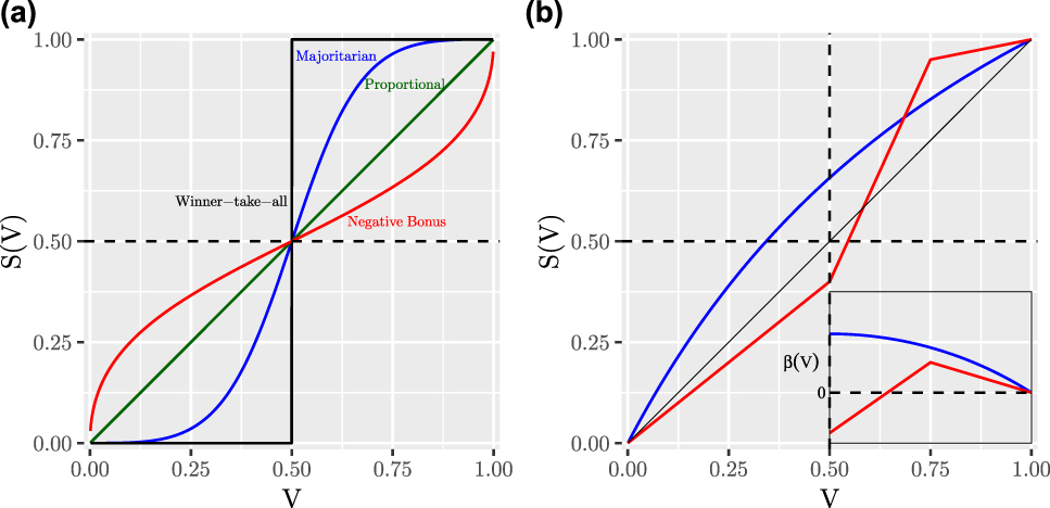
Four ranges of electoral responsiveness that satisfy Definition 4 are often discussed, each of which we illustrate with a fair seats–votes curve in the left panel of Figure 1. First, proportional representation meets the partisan symmetric standard because S(V) = V and 1 − S(1 − V) = V, or in other words ρ(V) = 1 and β(V) = 0 for all V (green line in the figure). Legislatures with single member, plurality voting systems are not guaranteed to be proportional by law and tend to be majoritarian by empirical pattern, which means that they usually give a bonus to the party winning a majority of votes statewide, with 1 < ρ(V) < ∞ (see blue line). For example, suppose the Democrats receive V = 0.55 proportion of the average district vote statewide and, because of how the district lines are drawn, receive S(0.55) = 0.75 proportion of the seats. This is not proportional, but it would be fair according to partisan symmetry because the Republicans, when receiving 1 − V = 0.55 proportion of the vote, would also receive 1 − S(1 − 0.55) = 0.75 proportion of the seats. Third, a more extreme type of electoral system still meeting partisan symmetry is winner-take-all (with ρ → ∞), where the majority vote winner receives all of the seats (solid black line in the left panel of Figure 1). A final type of system that meets partisan symmetry is where the party winning a majority of votes receives a negative bonus (0 < ρ < 1); for example, if S(0.65) = 0.55 and 1 − S(1 − 0.65) = 0.55 (red line).

FIGURE 1.

Types of Seats–Votes Curves

Notes: Left panel: Symmetric (fair) curves with differing levels of electoral responsiveness. Right panel: Asymmetric (biased) curves, including one consistently biased toward the Democrats (blue) and one with biases favoring different parties depending on V (red); the inset graph is for β(V) for V ∈ [0.5, 1] with the vertical axis scaled to be the same as the main plot, and lines color coded to the seats-votes curves.

Although partisan symmetry is widely viewed as a required standard of fair electoral systems (absent other considerations; see Online Appendix B), different levels of electoral responsiveness may reasonably be chosen as preferable or appropriate for and by different people and governments. Many would prefer that their electoral system meet partisan symmetry but not be proportional, winner-take-all, or negative bonus, and so would impose the restrictions of an unbiased (β(V) = 0) majoritarian (1 < ρ < ∞) electoral system. Similarly, although no US state constitution rejects partisan symmetry, the constitutions differ in their requirements regarding electoral responsiveness. Some state constitutions require their redistricters to draw highly responsive districts, to encourage competitive elections and party change in office, whereas others encourage their redistricters to draw minimally responsive districts, which protects their incumbents, perhaps to help them gain experience or seniority and thus power on congressional committees. Brunell (Reference Brunell2010) even argues that less responsiveness (and thus less competitiveness) produces happier constituents (see also Gerber and Lewis Reference Gerber and Lewis2004, 1378).

We also distinguish between two types of electoral systems that deviate from partisan symmetry—(a) those biased consistently in favor of one party and (b) those that switch from biased in favor of one party to the other as V changes. The right panel of Figure 1 gives one example of each of these seats–votes curves, along with an inset graph at the lower right with β(V) plotted by V and color-coded to the corresponding seats–votes curve. The blue seats–votes curve indicates bias in favor of the Democratic party for every value of V, although by different amounts. We can see this by the corresponding blue line in the inset graph. For example, at V = 0.5, S(V) = 0.66, and so β(0.5) = (0.66 − 0.5)/2 = 0.08, which is also the height of the left end of the blue line in the inset graph (although numbers on the vertical axis of the inset graph have been removed to reduce clutter, distances from zero are the same as for the main graph). Whereas the blue β(V) line in the inset graph is always above zero, indicating consistent bias toward the Democrats for all V, the red line indicates bias toward the Republicans for V < 0.125 and toward Democrats for larger average district vote values. Partisan bias that switches parties with V is important to consider when using summary measures of bias to represent the entire seats–votes relationship (Grofman and Brunell Reference Grofman and Brunell2005). This type of seats–votes curve can also be the result of a gerrymandering strategy where the party in control draws district maps biased against it at values of V it sees as unlikely, so long as the same map has more bias in its favor at values of V in future elections it sees as likely.

Gerrymandering Goals

Consider an imaginary partisan gerrymanderer focused solely on advantaging the respective political party.^{Footnote 5} Partisan gerrymanderers use their knowledge of voter preferences and their ability to draw favorable redistricting plans to maximize their party’s seat share. Gerrymanderers do not necessarily care about voter support, the efficiency of the translation of votes into seats, partisan bias, electoral responsiveness, or differential turnout—unless it helps them win more seats.

We show that these goals, when mapped into the concepts of partisan bias and electoral responsiveness, can be either consistent with or the opposite of those commonly described in the literature. Consider four situations, each of which leads to a different optimization function, effect on symmetry, and goal for bias and responsiveness (see Cox and Katz Reference Cox and Katz1999, sec. 3.3, Friedman and Holden Reference Friedman and Holden2008; Puppe and Tasnadi Reference Puppe and Tasnadi2009).

First is when the gerrymanderer is running scared (Mann Reference Mann1978) and so is worried about what the party’s statewide voting support may be in future elections. Here, optimizing means trying to win maximal seats with a safe margin, to insulate the party from potentially unfavorable future partisan swings. In this case, optimizing means seeking high bias and low responsiveness. Operationally, the gerrymanderer may do this by “packing” overwhelming numbers of opposition party votes into a few otherwise unwinnable districts and “cracking” the remaining opposition voting strength across a large number of districts to win each by a smaller but sufficiently safe vote margin. High bias helps the party in control of redistricting and low responsiveness protects their incumbents by locking in these gains for future elections.

Second is the opposite situation where the gerrymanderer is confident of a statewide majority of votes and so tries to make each district a microcosm of the entire state (i.e., v _d = V for all d), producing a winner-take-all outcome overall (Cox and Katz Reference Cox and Katz2002). In other words, the goal is an electoral system with low bias and high responsiveness. The “low bias” result is the consequence of optimizing primarily for high responsiveness, without preparing for the highly improbable situation where V = 1 − V ^O. This situation involves neither packing nor cracking: If a Democratic gerrymanderer thinks his or her party can count on 55% of the total statewide vote, then packing, to give the Republicans a few seats, would be foolish and cracking, to win any seats by 50% plus a few votes, is irrelevant. Instead, the goal would be to win with v _d = 0.55 for all d. (Unless of course the gerrymanderer is overconfident about partisan swing and winds up losing all the districts; see Grofman and Brunell Reference Grofman and Brunell2005.)

Third is where a partisan gerrymanderer reaches agreement with the other party (perhaps imposed by a redistricting commission). The result is a bipartisan gerrymander, which winds up optimizing for low bias and low responsiveness. Bias would be low because it is a zero-sum compromise between the parties, and low responsiveness reduces uncertainty in future elections by locking in the deal and protecting incumbents in both parties.

Finally, we consider the logical possibility of high bias and high responsiveness which, as it turns out, is rarely feasible in practice because of the dependence between the two quantities, as when additional packing to increase bias almost by definition reduces responsiveness. We can see this empirically in most real districtings (which we will see at scale when we get to Figure 3). Also, under a strategic behavior assumption, this is rarely an optimal strategy (Cox and Katz Reference Cox and Katz2002).

Gerrymandering-Based Fairness Standards

We offer two ways of deriving a normative standard of partisan fairness from a purely partisan gerrymandering perspective.

First, consider as a thought experiment disallowing a redistricter to use knowledge of where its party’s supporters live. This idea, which is equivalent to randomly permuting party labels on voters or on the gerrymanderer’s voter forecasts, clearly removes intent to do harm. This step alone may be of value because human psychology and most judicial systems judge intentional harm more severely than accidental harm (Greene Reference Greene2009). However, because plans drawn without knowledge of party support are drawn randomly with respect to party, any plan can be selected regardless of the degree of bias, responsiveness, or any other feature. In other words, gerrymandering without the knowledge of party removes intent but not harm. In fact, one possible districting plan that can occur is identical to that drawn by a partisan gerrymanderer with full knowledge of where its party’s voters live. In summary, the absence of intentional unfairness is not the same as fairness.

Second, we compare the efficiency of each party’s translation of votes into seats. In one observed election, the Democratic party receives S(V ^O) seats given V ^O votes and the Republican party receives 1 − V ^O votes and 1 − S(V ^O) seats. Which of these parties has a better or more efficient translation of seats into votes? Unless it happens that V ^O = 1 − V ^O = 0.5, this is an apples to oranges comparison because of the two different starting points. Making the vote comparison between the two parties comparable in any one election can be accomplished by imposing a counterfactual assumption. We consider two possibilities.

One possibility is to make an assumption enabling us to estimate what would happen if the parties switched their vote proportions, so that the election result was 1 − V ^O rather than V ^O. This would allow us to estimate the unobserved seat proportion 1 − S(1 − V ^O) and compare it with S(V ^O). This of course leads exactly to partisan symmetry.

Second, we could try assuming away the differential meaning of all, or some particular type of, votes cast for each party (e.g., “wasted votes,” which are those cast for the losing party in a district, and possibly also those above 0.5 plus one vote in winning districts; see the section on the efficiency gap below). However, although all votes are observed, asserting that all or any subset has the same meaning for each party, when the parties have different expected vote proportions, requires an assumption with the same ontological status as imagining partisan swings that lead to partisan symmetry. For example, suppose the Democrats receive V ^O = 0.6 and are confident of a statewide majority in subsequent elections under the same redistricting plan. Then, the votes cast for each party in specific districts have markedly different meanings for Democrats than for Republicans now in the minority, with 1 − V ^O = 0.4 votes. The Democrats in this scenario would benefit from districts that look like a microcosm of the state, whereas Republicans would benefit most by packing and cracking, and so assuming that these votes have the same meaning would be a stretch at best. Clearly, this does not seem like a promising direction for developing a new standard for partisan fairness.

No Additional Assumptions

In what is usually the best case, where we have five elections occurring between the decennial censuses and thus which we could consider (close to being) under the same electoral system, we observe five data points $\left\{ {\hat{S}\left( {V_t^{\rm{O}}} \right),V_t^{\rm{O}}:t = 1, \ldots ,\;5} \right\}$, where the observed statewide seat proportion $\hat{S}\left( {V_t^{\rm{O}}} \right)$ is an estimate of the expected value $S\left( {V_t^{\rm{O}}} \right)$ in election t.

From these data, two unusual circumstances may enable one to compute partisan bias with no modeling assumptions. In the first, if we happen to observe an election with a tied average district vote, V ^O = 0.5, then β(0.5) is estimable simply by the observed seat proportion. In the second, an even luckier situation (encompassing the first), two elections happen to be observed under the same electoral system with average district vote proportions symmetric around 0.5. For example, in Wisconsin State House elections run under the same redistricting plan, V ^O = 1 − 0.48 in 2012 and V ^O = 0.48 in 2014 and where, as a result, statewide seat proportions were observed in each election. In this particular case, the results indicate severe bias favoring the Republicans because of the dramatic seat proportion differences: $1 - \hat{S}\left( {1 - 0.48} \right) = 0.6$ but $\hat{S}\left( {0.48} \right) = 0.36$ (approximately), and so $\hat{\beta }\left( {0.48} \right) = - 0.12$. (This election was the subject of the Supreme Court case, Gill v Whitford, 585 US (2018).)

Functional Form Assumptions

One type of assumption is to specify a class of parametric functional forms for the seats–votes relationship and to estimate its parameters. Two examples of this form are linear (Tufte Reference Tufte1973),

(2)$$S\left(V \right) = {\alpha _0} + {\alpha _1}V,$$

and (redefining parameters α ₀ and α ₁) bilogit (King and Browning Reference King and Browning1987):

(3)$$S\left(V \right) = {1 \over {1 + \exp \left[ { - {\alpha _0} - {\alpha _1}\ln \left( {{V \over {1 - V}}} \right)} \right]}}.$$

In each equation, α ₀ and α ₁ are related in different ways to partisan bias and electoral responsiveness, respectively (and because S(V) in each expression is an expected value, real data need not fit either form exactly). For example, we drew the fair seats–votes curves in Figure 1 with α ₀ = 0 for all four and α ₁ = {0.5, 1, 3, 10,000} (10,000 being sufficiently close, for our figure, to winner-take-all, which is α ₁ → ∞).

Once we estimate the seats–votes curve, we can then read off point estimates of S(V) given any chosen V. This method enables one to compute partisan bias or any quantity of interest from the resulting estimated curve, along the appropriate level of uncertainty. Unfortunately, the few available observations from any one redistricting plan means that the result is usually uncertain and model dependent (and nonparametric approaches are not useful). As such, this strategy tends to be used more often for academic study of broad patterns across many electoral systems than for practical use evaluating individual redistrictings.

Partisan Swing Assumptions

An alternative approach is to use as inputs the district-level vote proportions. From this, we can estimate a single point on the seats–votes curve, S(V ^O), at the observed statewide vote V ^O and then we can add an assumption to generate hypothetical elections from the same electoral system, for different V.

Fortunately, patterns in electoral data throughout the US and most parts of the world can usually be decomposed into (a) the average partisan swing from one election to the next affecting all districts and (b) the relative ordering of district votes within any one election. Whereas (b) is highly predictable, statewide swings are more volatile and harder to predict. Fortunately, (b) is more important for evaluating redistricting than (a).

A simple and, we show, remarkably accurate assumption that identifies S(V) for any V is uniform partisan swing:

Assumption 3 [Uniform partisan swing (Butler Reference Butler and Nicholas1951)]. When the average district vote swings between elections under the same electoral system from V to V′, every district vote proportion moves uniformly by δ ≡ V′ − V, so that {v ₁,…, v _L} from one election becomes {v ₁ + δ,…, v _L + δ} in the next (with elements truncated to [0, 1] if necessary).

Of course, uniform partisan swing is obviously violated when it generates district vote proportions outside [0, 1], but this is superfluous detail. We thus restate the assumption: Given district-level vote proportions in one election, {v ₁,…, v _L}, and a chosen partisan swing parameter δ, the expected seat proportion in an election with average district vote V + δ under the same electoral system can be calculated via the (single-valued) function $S\left( {V + \delta } \right) = \mathop {{\rm{mean}}}_d \left[ {s\left( {{v_d} + \delta } \right)} \right]$.

To study the empirical accuracy of this seats–votes function, we would need to compute the out-of-sample error rate for the statewide seat proportion in one election identical in all respects to the previous one—including candidates, the campaign, spending, weather on election day, and patterns of incumbency—except for the statewide partisan swing and the usual random uncertainties in vote outcomes. Finding such pairs of observed elections is obviously impossible, and so we instead use successive elections within the same redistricting regime. The consequence is that our error rate approximates an upper bound for the actual errors of uniform partisan swing–based predictions.

We begin with data from all regular elections in US state legislatures 1968–2016. We narrow these to the 646 elections for legislatures with all single-member districts, at least 20 total districts, with at least half the seats contested, and where no redistricting has occurred between this election and the one before.^{Footnote 6}

Thus, for each of 646 elections, we use the district-level vote proportions in election 1; the statewide swing to election 2, $\delta = V_2^{\rm{O}} - V_1^{\rm{O}}$; and the uniform partisan swing assumption to predict the expected statewide seat proportion for election 2, ${S_2}\left( {V_2^{\rm{O}}} \right)$. We do not observe this expected value and so use the observed election 2 seat share ${\hat{S}_2}\left( {V_2^{\rm{O}}} \right)$ (as a model-free estimate of the expected value) for validation. The error metric for the prediction ${\hat{S}_1}\left( {V_2^{\rm{O}}} \right)$ is then simply ${\hat{S}_2}\left( {V_2^{\rm{O}}} \right) - {\hat{S}_1}\left( {V_2^{\rm{O}}} \right)$.

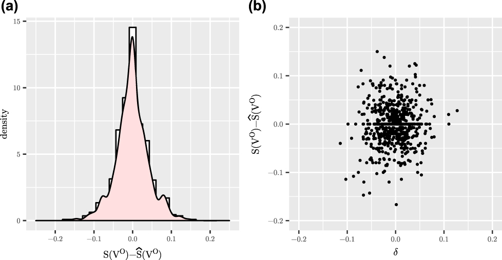
The left panel of Figure 2 gives a histogram of these out-of-sample prediction errors from uniform partisan swing. These results reveal highly accurate predictions, with a median error of 0.0000, a mean error of −0.001 (one-10th of one percentage point), and an interquartile range of only [−0.025, 0.021]. And these numbers are upper bounds.^{Footnote 7}

FIGURE 2.

Error Rates of Out-Of-Sample Statewide Seat Proportion Predictions Based on the Assumption of Uniform Partisan Swing

Notes: Histogram of errors (left panel) and errors by statewide partisan swing, δ, from one observed election to the next in predicting the seat proportion.

We also use these data to study how fast uniform partisan swing–based predictions degrade as we extrapolate farther from the original data, that is, when the statewide vote swing is larger. The right panel of Figure 2 plots the prediction error by the size of the statewide vote swing, δ. Remarkably, the graph shows that predictions do not degrade at all for larger swings (i.e., as δ deviates from zero). The implication is that uniform partisan swing is a relatively fixed feature of elections, with the more difficult-to-predict component of elections mostly relegated to statewide voter swings, which happen not to be important for studying partisan symmetry.

In our data, and in many elections all over the world, uniform partisan swing is a reasonable first approximation, especially for theoretical purposes like ours. What Assumption 3 ignores is that the world is stochastic and so is less useful for some empirical purposes. The simplicity can also generate inefficiency in part because of discreteness (Nagle Reference Nagle2015, 351). We thus generalize the deterministic uniform partisan swing assumption either directly via stochastic modeling (King Reference King1989) or statistical modeling:

Assumption 4 [Stochastic uniform partisan swing (Gelman and King Reference Gelman and King1994a)]. Hypothetical (denoted “(hyp)”) district-level vote proportions, under the same electoral system, are generated as

(4)$$v_d^{\left( {{\rm{hyp}}} \right)} = {X_d}\theta + {\gamma _d} + {\delta ^{\left( {{\rm{hyp}}} \right)}} + \epsilon _d^{\left( {{\rm{hyp}}} \right)},$$

where X _d is a vector of covariates describing the districts, candidates, voters, and lagged vote; θ is a vector of effect parameters; γ _d is an independent random normal district effect that is constant over hypothetical elections but varying over districts; δ ^(hyp) is the researcher-chosen uniform swing; and $\epsilon _d^{\left( {{\rm{hyp}}} \right)}$ is a stochastic normal error term, independent of γ and over d.

Assumption 4, rewritten as we did with its special case in Assumption 3, is thus less restrictive, more realistic, and more statistically efficient, and so should be used whenever it makes a difference. For our theoretical and methodological purposes, we will usually use the simpler Assumption 3 in this article to ease exposition, and because we analyze so many districts that inefficiency is a minor issue and because relevant empirical patterns of voter behavior are extremely regular across most elections in most countries (King et al. Reference King, Rosen, Tanner and Wagner2008, 952).

Estimation from Seats–Votes Curves

A straightforward way to estimate a feature of the seats–votes curve is with an estimate of the entire curve, using one of the assumptions in the section on estimation above. With the full curve, partisan bias β(V), electoral responsiveness ρ(V), and other quantities are easy to estimate for any relevant V ∈ [0, 1], ensuring that Assumptions 1 and 2 hold. A few of the important articles computing bias and responsiveness in this way include Brunell (Reference Brunell1999) and Jackman (Reference Jackman1994), which use Assumption 4; Erikson (Reference Erikson1972), using the functional form assumption in equation 2; Gilligan and Matsusaka (Reference Gilligan and Matsusaka1999) and Niemi and Jackman (Reference Niemi and Jackman1991), using the functional form assumption in equation 3; and Brady and Grofman (Reference Brady and Grofman1991) and Garand and Parent (Reference Garand and Parent1991), which use a combination of the functional form assumption in equation 3 along with Assumption 3.

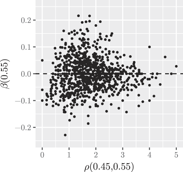
As an illustration, we estimate partisan bias and electoral responsiveness using data from 963 legislatures (those from 1968 to 2016 with all single-member districts, at least 20 seats, and at least half of the seats are contested) via Assumption 3. Figure 3 plots bias vertically by responsiveness horizontally, both for V ∈ [0.45, 0.55]. The scatterplot shows that bulk of bias results is in [−0.1, 0.1] and responsiveness in [1, 3]. The two quantities are uncorrelated in these data, but not independent in that as ρ increases, |β| declines. This pattern is consistent with the scenario from the section on Gerrymandering Goals, where the redistricter is confident of a statewide majority and so seeks high responsiveness and is left with low bias.

FIGURE 3.

Estimates of Partisan Bias and Electoral Responsiveness, Both Evaluated in the Range V ∈ [0.45, 0.55] in 963 Legislatures

Proportional Representation

We now discuss several individual measures that do not first estimate the entire seats–votes curve. For expository reasons, we begin with the simple deviation from proportional representation measure, PRD(V ^O) = S(V ^O) − V ^O, which is easy to understand and turns out to fail as a measure of partisan fairness. We explain and then show how it is useful for other purposes.

Under this approach’s standard of fairness, PRD(V) = 0, we solve for expected seats as a function of votes, S(V ^O) = V ^O, and then swap V ^O with V, yielding S(V) = V. This is a coherent seats–votes curve because each value of V produces one value of S(V), with Assumptions 1 and 2. See the green line in Figure 1, a symmetric electoral system with ρ(V) = 1, for all V. By writing partisan bias as β(V) = {S(V) − [1 − S(1 − V)]}/2 = {PRD(V) + PRD(1 − V)}/2, we can see that the proportional representation standard is a special case of partisan symmetry (because PRD(V) = PRD(1 − V) = 0 implies β(V) = 0 for all V), but partisan symmetry is not a special case of proportional representation (because β(V) = 0 whenever PRD(V) = PRD(1 − V), even if PRD(V) ≠ 0; see the other lines in Figure 1).

Although the proportional representation standard of PRD(V ^O) = 0 is theoretically coherent, PRD(V ^O) is inadequate as a measure of partisan symmetry. The problem is that V ^O and S(V ^O) produce only a single model-free estimate of a point on the seats–votes curve, which is insufficient for estimating the entire curve, because the second term in β(V ^O) = [PRD(V ^O) + PRD(1 − V ^O)]/2 is unobserved without further assumptions. For example, the election outcome S(0.6) = 0.6 is consistent with the standard because it falls on the line S(V) = V, which is proportional and symmetric. However, the same observed point is also consistent with the flat line S(V) = 0.6 (for all V) or with 1 − S(1 − 0.6) = 0, neither of which is proportional, symmetric, or fair.

The deviation from proportional representation in one election is thus not a general measure of partisan symmetry, but it can be informative about its more specific standard (β(V) = 0 such that ρ(V) = 1): Although PRD(V ^O) = 0 offers no information one way or the other, PRD(V ^O) ≠ 0 implies that this specific standard should be rejected. This may be useful on its own, but to go further requires estimating other points on the seats–votes curve, perhaps via the assumptions from the section above on estimation.

However, even when completely uninformative about partisan symmetry, PRD(V ^O) is still an interesting and politically relevant summary of the outcome of an election. Certainly, small minority parties want to know whether they will receive at least some seats and so may compare it to their vote proportion as at least a benchmark. A forecast of PRD(V ^O) would likely influence whether a small minority party would even compete in many districts or be likely to attract significant campaign contributions.^{Footnote 8}

Mean–Median

The mean–median measure is an easy-to-calculate difference: MM = V ^O − M, where V ^O is the average district vote and M is the median district vote, implicitly defined as ${1 \over L}\sum\limits_{{v_d} > M} {1 = {1 \over 2}}$. Fairness according to this measure is when MM = 0. The measure is claimed “to reliably assess [partisan] asymmetry in state-level districting schemes” (Wang Reference Wang2016a, 367). Essentially the same claim appears in Wang (Reference Wang2016b), Krasno et al. (Reference Krasno, Magleby, McDonald, Donahue and Best2018), and McDonald and Best (Reference McDonald and Best2015), among others. Although no proof of this claim has appeared in the literature, we show that it is correct in different ways for two distinct theoretical quantities, vote- and seat-denominated partisan bias. In the first, we prove that MM provides limited information about β(V); in the second, we show that MM is a more useful measure of a new theoretical quantity.

A Limited Measure of Partisan Bias

We begin by showing, under Assumptions 1, 2, and 3, that MM = 0 if and only if $\hat{\beta }\left( {0.5} \right) = 0$. Formally,

(5)$$\hat{\beta }\left( {0.5} \right) = \hat{S}\left( {0.5} \right) - 0.5\quad \left( {{\rm{by}}\;{\rm{definition}}} \right),$$

$$= {{\mathop \sum \nolimits_{{v_d} > {V^{\rm{O}}}} 1} \over L} - 0.5\quad \left( {{\rm{Assumption}}\;3} \right),$$

(6)$$= {{\mathop \sum \nolimits_{{v_d} > M} 1} \over L} - 0.5\quad \left( {{\rm{Assuming}}\;{\rm{MM}} = 0} \right),$$

$$= 0.5 - 0.5 = 0.</tex-math></alternatives> \quad\quad\quad\quad\quad\quad\quad\quad\quad\quad\quad\quad&#x2610;</disp-formula></p><p>As an estimate of <italic>&#x3b2;</italic>(0.5), the mean&#x2013;median measure has two limitations (in addition to the effects of discreteness; Nagle <xref ref-type="bibr" rid="ref52">2015</xref>). First, although our proof shows that MM is a useful indicator for whether <italic>&#x3b2;</italic>(0.5) is zero, and so could be used for a hypothesis test, it is not a general measure of <italic>&#x3b2;</italic>(0.5), as we have no proof that it is an unbiased or consistent estimator because the magnitude is not known to be correct when other than zero.</p><p>Second, if the electoral system is biased at a point other than <italic>V</italic> &#x3d; 0.5, the mean&#x2013;median measure will not necessarily reflect overall partisan symmetry (see the right panel, <xref ref-type="fig" rid="fig1">Figure 1</xref>). Consider an election with 10 districts and the following vote proportions:<disp-formula id="eqn7"><label>7</label><alternatives><graphic xlink:href="S000305541900056X_eqn7" mime-subtype="gif"/><tex-math><![CDATA[$$\left\{ {0.48,0.49,0.49,0.49,0.59,0.61,0.65,0.65,0.65,0.90} \right\}.$$

From these data, and the assumptions above, ${\rm{mm}} = \hat{\beta }\left( {0.5} \right) = 0$, which would enable us to conclude that an aspect of the electoral system is fair. However, without any additional assumptions, we can show that in fact other aspects of the electoral system can be biased. For example, if the Democratic party receives an average district vote of V ^O = 0.6 (the observed value of these district proportions), they would win a $\hat{S}\left( {{V^{\rm{O}}}} \right) = 0.6$ seat proportion, but when the Republicans receive the same 1 − V ^O = 0.6, they would win a remarkable $1 - \hat{S}\left( {1 - {V^{\rm{O}}}} \right) = 0.9$ of the seats, a 30 percentage point difference. This means that $\hat{\beta }\left( {0.6} \right) = - 0.15$. In this example, the mean–median measure indicates that the electoral system represented is fair, but it is instead quite unfair.

A Better Measure of “Vote-Denominated” Partisan Bias

More interestingly, we can prove that MM is a valid estimator of a new theoretical quantity, “vote-denominated” partisan bias VDB(0.5): how much more one party must earn in votes than the other party to win a given seat proportion (defined more formally in Online Appendix F). With Assumptions 1, 2, and 3, we have

$${\rm{VDB}}\left( {0.5} \right) = - {{\left\{ {V\left(S \right) - \left[ {1 - V\left( {1 - S} \right)} \right]} \right\}} / 2}\quad \left( {{\rm{by}}\;{\rm{definition}}} \right),$$

$$= 0.5 - V\left( {0.5} \right),$$

$$= V - M\quad \left( {{\rm{Assumption}}\;3} \right),$$

$$\equiv \,{\rm{MM}}. \quad&#x2610;$$

If we use the more realistic Assumption 4 in place of Assumption 3, it is easy to show that MM is a statistically consistent estimator of VDB(0.5). Either way, this proof is important because, although the magnitude of MM has no clear relationship to β(0.5), it is correct for the alternative quantity VDB(0.5), making the mean–median measure an easy-to-calculate and accurate estimator of this unusual but still coherent theoretical quantity.

Lopsided Outcomes

Wang introduces the lopsided outcomes test and claims it can be used “to reliably assess [partisan] asymmetry in state-level districting schemes,” (Wang Reference Wang2016b, 1263), or “to detect…” or “identify partisan asymmetry” (Wang Reference Wang2016a, 368). We show here that this claim is false, and along the way describe other more productive uses of the measure.

Begin by denoting the average Democratic vote in Democratic-won districts as $D = {{\mathop \sum _d s\left( {{v_d}} \right){v_d}} / {\mathop \sum _d s\left( {{v_d}} \right)}}$ and the average Democratic vote in Republican-won districts as $R = {{\mathop \sum _d \left[ {1 - s\left( {{v_d}} \right)} \right]{v_d}} / {\mathop \sum _d \left[ {1 - s\left( {{v_d}} \right)} \right]}}$, which implies R < 0.5 < D. Then we write an accounting identity with the average district vote as a weighted average of Democratic and Republican seat shares, V = S(V ^O)D + [1 − S(V ^O)]R, and solve for the generic seats–votes relationship, all without assumptions:

(8)$$S\left( {{V^{\rm{O}}}} \right) = {{{V^{\rm{O}}} - R} \over {D - R}}.$$

Equation 8 is true by definition, but swapping V ^O for V is not sufficient to define a coherent seats–votes curve because S(V) is not single-valued. The presence of R and D on the right side, which are functions of V, means that we need more constraints to ensure S(V) has only one value. Only at that point can we add Assumption 2 and evaluate the claim that the resulting seats–votes curve meets the partisan symmetry standard. So the question for any measure is whether it imposes these sufficient constraints.

The lopsided outcomes measure is defined as the simple party difference in the average win size:

(9)$${\rm{lo}} = D - \left( {1 - R} \right).$$

This measure seems intuitive because packed districts are sometimes a characteristic of successful partisan gerrymandering but, as we showed above, the intuition is often wrong because packing (and cracking) can be counterproductive. The measure deserves credit as a fine measure of the skewness of the vote proportion distribution because nonskewness implies that the center of mass on either side of v _d = 0.5 will be equidistant from this midpoint. A forecast of this measure may indeed be useful to partisans or others trying to understand the competitive playing field and what it takes on average to win a district for their party.

Unfortunately, lopsided outcomes is not necessarily related to partisan symmetry or any other measure of fairness. To show this, we now study how equation 9 is constrained by the measure’s notion of fairness, LO = 0. Thus, by substituting D = 1 − R into equation 8, we have

(10)$$S\left( {{V^{\rm{O}}}} \right) = {{{V^{\rm{O}}} - R} \over {1 - 2R}}.$$

Unfortunately, after substituting V ^O with V, we are still left with multiple values of S(V) for any one V because of the presence of R on the right side, which indicates the lack of a coherent seats–votes curve. This means that the lopsided outcomes test, and the implied set of multiple seats–votes curves it considers “fair,” can be consistent with either symmetry or asymmetry. As a result, LO does not imply particular values of β(V) and is not a measure of (the deviation from) partisan symmetry.

Thus, to construct an example, we add information the framework omits in the form of Assumption 3. We then construct examples of votes from three hypothetical legislatures:

(11)$$\left\{ {0.25,0.25,0.25,0.75,0.75,0.75,0.75,0.75,0.75,0.75} \right\},$$

(12)$$\left\{ {0.30,0.30,0.40,0.55,0.55,0.65,0.65,0.90,0.90,1} \right\},$$

(13)$$\left\{ {0.40,0.40,0.40,0.40,0.40,0.60,0.60,0.60,0.60,0.60} \right\},$$

and then compute partisan bias and LO for each. The inconsistency is apparent: Legislature (11) is judged fair by the lopsided outcomes test but is in fact asymmetric (LO = 0, $\hat{\beta }\left( {{V^{\rm{O}}}} \right) = \hat{\beta }\left( {0.5} \right) = 0.2$). Legislature (12) is judged unfair by lopsided outcomes but is in fact symmetric (LO = 0.08, $\hat{\beta }\left( {{V^{\rm{O}}}} \right) = \hat{\beta }\left( {0.5} \right) = 0$). And Legislature (13) is also judged fair by lopsided outcomes and is in fact symmetric (LO = 0, $\hat{\beta }\left( {{V^{\rm{O}}}} \right) = 0$).

Declination

Warrington (Reference Warrington2018a, 2) introduced a measure called declination and claims it “is a measure of partisan symmetry” (or “a new measure of partisan asymmetry”; Warrington Reference Warrington2018b). We prove that this claim is incorrect, but along the way convey the measure’s intuition and potential descriptive uses.

Warrington found a clever geometric interpretation of his measure, intuitive from the perspective of his field of mathematics, by defining it as DECLINATION = 2(θ _D − θ _R)/π, where θ _D = arctan[(2D − 1)/S(V ^O)] and θ _R = arctan{(1 − 2R)/[1 − S(V ^O)]}. For our intended audiences, the measure is easier to understand without the arctan transformation or constant normalizations, which only adjust the scale. We thus define the un-normalized declination

(14)$${\rm\sc{DEC}} = {{D - 0.5} \over {S\left( {{V^{\rm{O}}}} \right)}} - {{0.5 - R} \over {1 - S\left( {{V^{\rm{O}}}} \right)}}.$$

Equation 14 (which can also be thought of as a normalized version of lopsided outcomes; cf. equation 9) is similar to the difference in the magnitude of electoral responsiveness on each side of V = 0.5. This is important because under partisan symmetry, the difference in (actual) responsiveness is zero. The problem is that responsiveness is a change in votes divided by a change in seats (see Definition 3), whereas each of the two terms in DEC is a change in votes divided by an absolute seat proportion. That means that DEC is not an unbiased measure of partisan symmetry, but is related and serves as a measure of the skewness of the distribution of district vote proportions.

To formally prove the connection between declination and partisan symmetry, consider how its notion of fairness, DEC = 0, constrains the generic equation 8. The result is

(15)$$S\left( {{V^{\rm{O}}}} \right) = {{D - 0.5} \over {2D - 0.5 - {V^{\rm{O}}}}}.$$

As with lopsided outcomes, even after swapping V ^O for V, S(V) is not a single-valued function of V and so, even under its notion of “fairness,” is not a coherent seats–votes curve. That is, we can try to adjust V to see how S(V) changes, but how D changes with V is left unspecified, which leaves many possible values of S(V). The proposed standard is thus consistent with both symmetric and asymmetric seats–votes curves and, as such, declination not a measure of partisan symmetry.

In parallel to the previous section, we now offer examples of these inconsistencies with three hypothetical 10-district legislatures:

(16)$$\left\{ {0.45,0.45,0.55,0.55,0.55,0.60,0.80,0.80,0.80,0.95} \right\},$$

(17)$$\left\{ {0.40,0.40,0.55,0.55,0.55,0.60,0.60,0.63,0.70,0.70} \right\},$$

(18)$$\left\{ {0.48,0.48,0.52,0.52,0.55,0.59,0.60,0.60,0.63,0.63} \right\}.$$

As in the previous section, we add missing information in the form of Assumption 3 and compute partisan bias and DEC. We find that Legislature (16) is judged fair by declination but is in fact asymmetric (DEC = 0, $\hat{\beta }\left( {{V^{\rm{O}}}} \right) = \hat{\beta }\left( {0.5} \right) = - 0.1$. Legislature (17) is judged unfair by declination but is in fact symmetric (DEC = −0.36, $\hat{\beta }\left( {0.5} \right) = \hat{\beta }\left( {{V^{\rm{O}}}} \right) = 0$). And Legislature (18) is also judged fair by declination and is symmetric (DEC = 0, $\hat{\beta }\left( {0.5} \right) = \hat{\beta }\left( {{V^{\rm{O}}}} \right) = 0$).

Efficiency Gap

Stephanopoulos and McGhee (Reference Stephanopoulos and McGhee2015) introduce the efficiency gap and claim it is “a new measure of partisan [a]symmetry” (quote repeated on pages 831, 834, 838, 849, and 899). We prove that this claim is false, and also convey the intuition and productive uses of the measure.

The efficiency gap redefines the classic definition of “wasted votes” of all votes cast for losing candidates (Campbell Reference Campbell1996) by adding those for winning candidates above the 50%-plus-one-vote threshold. The article then claims that partisan symmetry is satisfied when these wasted votes are equally divided between the parties. We show this claim is incorrect. Although the efficiency gap is controversial (Chambers, Miller, and Sobel Reference Chambers, Miller and Sobel2017; Cho Reference Cho2017; Tapp Reference Tapp2018), it comes with important intuition; the authors also deserve substantial credit for bringing many, including the US Supreme Court, back to this venerable field (see Gill v. Whitford, 585 US (Reference Lander2018); see Stephanopoulos and McGhee Reference Stephanopoulos and McGhee2018).

The intuition works best in highly competitive situations, when one party is in control of redistricting and running scared. Here, redistricters try to pack and crack and thus reduce wasted votes. In other situations, such as when confident of a statewide vote majority, packing is against the redistricter’s interests. Here, the efficiency gap becomes confused; for example, if a party receives 80% of the votes and all the seats, the measure indicates that the electoral system treats it unfairly (see also Veomett Reference Veomett2018).

To formalize, denote the proportion of wasted votes in district d for Democrats as w _d = v _d − s(v _d)/2 ∈ [0, 0.5] and Republicans as (0.5 − w _d) = (1 − v _d) − [1 − s(v _d)]/2. Then define the efficiency gap as follows:

(19)$${\rm{EG}}\left( {{V^{\rm{O}}}} \right) = {{\sum\limits_d {{n_d}\left( {0.5 - {w_d}} \right)} - \sum\limits_d {{n_d}{w_d}} } \over {\sum\limits_d {{n_d}} }},$$

(20)$$= S\left( {{V^{\rm{O}}}} \right) - 2{V^{\rm{O}}} + 0.5 - C,\;{\rm{where}}\;C = 2{{\sum\limits_d {{t_d}{w_d}} } \over {\sum\limits_d {{n_d}} }},$$

where ${t_d} = {n_d} - \mathop {{\rm{mean}}}_d \left( {{n_d}} \right)$ (see McGhee Reference McGhee2017). We can solve this expression as S(V ^O) = 2V ^O − 0.5 + C. However, because C is a function of V, a single-valued seats–votes function does not result, violating Assumption 1. Stephanopoulos and McGhee (Reference Stephanopoulos and McGhee2015, 853) tried to remove the problem by assuming the turnout is constant, implying C = 0, but because this claim is observable, making it an “assumption” does not make sense. A minimally necessary condition for which C = 0 is Cov(t _d, w _d) = 0, but this too does not solve the problem because this covariance is rarely zero.

This result means that the claims for the efficiency gap are mistaken: it is not a measure of partisan symmetry. The slope of the implied seats–votes curve is not two because it does not imply a coherent seats–votes curve. The claim that the efficiency gap and partisan bias “are mathematically identical in the special case in which both parties receive exactly 50% of the vote” (p. 856) is incorrect. The claim that “a party can win more than half the seats with half the votes only by exacerbating the efficiency gap in its favor” (p. 856) is also untrue.

Corrected Efficiency Gap

We give the efficiency gap idea the benefit of the doubt here with the same simplicity sought in Stephanopoulos and McGhee (Reference Stephanopoulos and McGhee2015) by computing a corrected efficiency gap (CEG). This measure involves moving C to the left side of equation 20, and defining:

(21)$${\rm{CEG}}\left( {{V^{\rm{O}}}} \right) \,\equiv\, {\rm{EG}}\left( {{V^{\rm{O}}}} \right) + C = S\left( {{V^{\rm{O}}}} \right) - 2{V^{\rm{O}}} + 0.5.$$

(cf. McGhee Reference McGhee2017, 427ff). We study this measure’s standard of fairness CEG(V ^O) = 0 by solving equation 21 for S(V), adding Assumptions 1 and 2, and writing what turns out to be a coherent (single-valued) seats–votes curve:

(22)$$S\left(V \right) = 2V - 0.5.$$

The assumed fair seats–votes curve in equation 22 meets the partisan symmetry standard in Definition 1 because S(V) = 2V − 0.5 = 1 − [2(1 − V) − 0.5], but it is a special case because of the additional constraints of a slope of ρ(V) = 2 for V ∈ [0.25, 0.75] and ρ(V) = 0 for V ∉ [0.25, 0.75] (the red line in the left panel of the figure in Online Appendix G); note that all four symmetric electoral systems in Figure 1 would be judged unfair according to this standard. Equation 22 is an unpopular normative standard (e.g., Chambers, Miller, and Sobel Reference Chambers, Miller and Sobel2017, 16; McGann et al. Reference McGann, Smith, Latner and Keena2015, fn. 1), but it is coherent and so meets Assumption 1.

We move now from the fair seats–votes curve assumed under the efficiency gap framework to estimation. Unfortunately, an estimated CEG in one election is insufficient to determine whether the electoral system is symmetric. In particular, β(V ^O) = [CEG(V ^O) + CEG(1 − V ^O)]/2 equals zero only when CEG(V ^O) = −CEG(1 − V ^O). However, an election with 1 − V ^O is unobserved and so CEG(1 − V ^O) is not identified, nor is β(0.5) or β(V).

Examples and empirical evidence about CEG are given in Online Appendix G.

Simulation Measures

Simulation measures seek to compare a redistricting plan with all possible plans for a state, or all that meet the chosen criteria (Chen and Rodden Reference Chen and Rodden2013; Chikina, Frieze, and Pegden Reference Chikina, Frieze and Pegden2017; Duchin Reference Duchin2018; Magleby and Mosesson Reference Magleby and Mosesson2018). Unfortunately, all possible plans are too large, proper random sampling remains an unsolved problem (Fifield et al. Reference Fifield, Higgins, Imai and Tarr2018; Tam Cho and Rubinstein-Salzedo Reference Tam Cho and Rubinstein-Salzedo2019), and using actual plans from different states is unrealistic (Wang Reference Wang2016b).

We thus describe two simulation-based measures (for when the random sampling problem is solved) without separately defined standards and then two with clear standards. First, purely relative measures are of little value: Is a plan fair if it is at the 50th percentile of possible plans but, when the parties split the vote equally, Republicans receive 85% of the seats? Is a plan unfair if a party receives more seats than 99.99% of all plans but, when the parties split the votes equally, they split the seats equally? This approach might work if achieving a fairer plan on an absolute scale were known to be impossible, but that is rare in real redistrictings and in any event is not addressed by relative measures.

Second, some assign uniform probability to each randomly drawn plan. The resulting distribution has been compared with estimating the “cone of uncertainty” in hurricane predictions (Lander Reference Lander2018), but this analogy does not hold. The cone of uncertainty is a posterior distribution based on informative data, whereas a uniform distribution is a prior assumed without evidence (based on something like Laplace’s discredited “Principle of Insufficient Reason”). Uniform hurricane predictions would put equal probability over the entire globe. In real redistricting cases, when (naive) judges or special masters propose drawing plans randomly, or arbitrarily like a checkerboard, experts on all sides strenuously object because of the well-known likelihood of unintended consequences.

We also consider two approaches that make good use of randomly drawn districts. First, sampling can be productively used for “producing a large set of legally viable maps with respect to multiple criteria” (Cain et al. Reference Cain, Tam Cho, Liu and Zhang2017, 1538) to convey what is possible, such as plans with de minimis levels of partisan bias while also meeting other criteria. The approach is also useful for identifying the characteristics of plans that are impossible given the state’s geography, which can be compelling (e.g., Chen and Rodden Reference Chen and Rodden2013, sec. 5 and Duchin et al. n.d.). These deterministic statements are also useful for studying what constrains gerrymanderers, such as compactness or the tendency of Democrats to live packed in cities; after all, there is no reason to think gerrymanderers are influenced by any number of possible plans except for the one they would choose as optimal.

Finally, suppose a redistricter claims that the only criteria used in selecting a plan were (say) compactness and equal population. Then choice among plans that meet these criteria is random (due to exchangeability). This leads to a coherent hypothesis test: For a criterion outside the original two, such as partisan bias, the null—that no information was used in drawing the plan other than the three criteria—can be computed directly by computing the probability of observing partisan bias as or more extreme than the existing plan. One may also be able to develop a coherent hypothesis test by drawing plans from distributions like $f\left( {\hat{\beta }\left( {0.5} \right)\,|\,\beta \left( {0.5} \right) = 0} \right)$. Although this density is not identified from uniform draws, it would be useful if we can develop a way to draw from the null directly.