1. Introduction
As first demonstrated two decades ago (Clark et al. Reference Clark, Krushelnick, Davies, Zepf, Tatarakis, Beg, Machacek, Norreys, Santala and Watts2000; Maksimchuk et al. Reference Maksimchuk, Gu, Flippo, Umstadter and Bychenkov2000; Snavely et al. Reference Snavely, Key, Hatchett, Cowan, Roth, Phillips, Stoyer, Henry, Sangster and Singh2000), the interaction of an ultraintense ( $I_L\gtrsim 10^{18}\ \text {W cm}^{-2}$) laser pulse with a thin (
 ${\sim }1\ \mathrm {\mu }$m) foil target results in the formation of an energetic ion beam through the so-called target normal sheath acceleration (TNSA) mechanism (Wilks et al. Reference Wilks, Langdon, Cowan, Roth, Singh, Hatchett, Key, Pennington, MacKinnon and Snavely2001). Stimulated by a great variety of applications, ranging from radiography (Borghesi et al. Reference Borghesi, Campbell, Schiavi, Haines, Willi, MacKinnon, Patel, Gizzi, Galimberti and Clarke2002) and warm dense matter (Patel et al. Reference Patel, Mackinnon, Key, Cowan, Foord, Allen, Price, Ruhl, Springer and Stephens2003) to nuclear physics (Ledingham, McKenna & Singhal Reference Ledingham, McKenna and Singhal2003) and proton therapy (Malka et al. Reference Malka, Faure, Gauduel, Lefebvre, Rousse and Phuoc2008), vast research effort has since been devoted to improving the maximum energy, flux and collimation of the ion beam. In the meantime, other acceleration mechanisms have been proposed, such as radiation pressure acceleration (Macchi et al. Reference Macchi, Cattani, Liseykina and Cornolti2005; Schlegel et al. Reference Schlegel, Naumova, Tikhonchuk, Labaune, Sokolov and Mourou2009), light sail acceleration (Esirkepov et al. Reference Esirkepov, Borghesi, Bulanov, Mourou and Tajima2004; Klimo et al. Reference Klimo, Psikal, Limpouch and Tikhonchuk2008; Robinson et al. Reference Robinson, Zepf, Kar, Evans and Bellei2008; Macchi, Veghini & Pegoraro Reference Macchi, Veghini and Pegoraro2009; Qiao et al. Reference Qiao, Kar, Geissler, Gibbon, Zepf and Borghesi2012), relativistic self-induced transparency acceleration (d'Humières et al. Reference d'Humières, Lefebvre, Gremillet and Malka2005; Esirkepov, Yamagiwa & Tajima Reference Esirkepov, Yamagiwa and Tajima2006), breakout afterburner (Yin et al. Reference Yin, Albright, Hegelich, Bowers, Flippo, Kwan and Fernández2007, Reference Yin, Albright, Bowers, Jung, Fernández and Hegelich2011), collisionless shock acceleration (Denavit Reference Denavit1992; Silva et al. Reference Silva, Marti, Davies, Fonseca, Ren, Tsung and Mori2004; Fiuza et al. Reference Fiuza, Fonseca, Tonge, Mori and Silva2012; Haberberger et al. Reference Haberberger, Tochitsky, Fiuza, Gong, Fonseca, Silva, Mori and Joshi2012) or magnetic vortex acceleration (Fukuda et al. Reference Fukuda, Faenov, Tampo, Pikuz, Nakamura, Kando, Hayashi, Yogo, Sakaki and Kameshima2009; Nakamura et al. Reference Nakamura, Bulanov, Esirkepov and Kando2010). However promising these mechanisms may appear to be, they generally require stringent laser and target properties, rendering their experimental realization very challenging. Therefore, due to its simplicity and robustness, TNSA remains by far the most widely used method for laser-based ion acceleration, motivating extensive optimization efforts concerning target geometry and composition.
The TNSA proceeds from the strong electrostatic fields set-up at the target surfaces by the laser-driven hot electrons leaking out into vacuum, and forming negatively charged sheaths. Those fields act to reflect the hot electrons back into the target, while driving the outward expansion of the surface ions. Their strength scales as  $E_x \simeq k_B T_h/e \max (\lambda _{\textit{Dh}},L_n)$, with
 $e$ being the elementary charge,
 $k_B$ the Boltzmann constant,
 $T_h$ the ‘temperature’ of the hot electrons,
 $\lambda _{\textit{Dh}}$ their local Debye length and
 $L_n$ the local ion density scale length (Mora Reference Mora2003). The sheath field is generally stronger at the target back side because it is not directly perturbed by the laser, and so is characterized by a sharper density gradient (
 $L_n \ll \lambda _{\textit{Dh}}$). In laser–solid interactions, the energy of the hot electrons is usually comparable with the ponderomotive potential,
 $T_h \simeq m_e c^{2} \sqrt {1+a_0^{2}/2}$, where
 $a_0 = eE_0/m_e c \omega _0$ is the dimensionless laser field (
 $\omega _0$ is the laser frequency,
 $m_e$ the electron mass and
 $c$ the velocity of light) (Wilks et al. Reference Wilks, Kruer, Tabak and Langdon1992). For the
 $10^{19}\text {--}10^{20}\ \text {W cm}^{-2}$ intensities commonly reached by present-day multi-100 TW systems, typical values of
 $T_h\sim 1\ \text {MeV}$,
 $\lambda _{\textit{Dh}} \sim 1\ \mathrm {\mu }$m are attained, generating electrostatic fields of a few
 $10^{6}$ V
 $\mathrm {\mu }$m
 $^{-1}$ which readily ionize the hydrogen-rich surface contaminants. Due to their largest charge-to-mass ratio, the surface protons react the fastest to the sheath field and are accelerated to the highest velocities. Apart from some aspects specific to hot-electron generation, the interplay of hot and bulk electrons and the usually multilayered and/or multispecies composition of the targets, TNSA is equivalent to the standard problem of plasma expansion into vacuum (Gurevich, Pariiskaya & Pitaevskii Reference Gurevich, Pariiskaya and Pitaevskii1966; Crow, Auer & Allen Reference Crow, Auer and Allen1975; Mora Reference Mora2003).
Since the accelerating field ( $E_x \simeq k_B T_h/\lambda _{Dh} \propto \sqrt {n_h T_h}$) at a sharp interface increases with the temperature (
 $T_h$) and density (
 $n_h$) of the hot electrons, various target configurations have been designed to maximize these parameters for a given laser drive. Among the explored setups, double-layer targets made of a thin solid foil preceded by a plasma layer of near-critical electron density offer particularly encouraging prospects, with up to threefold enhancement in cutoff ion energies being reported (Nakamura et al. Reference Nakamura, Tampo, Kodama, Bulanov and Kando2010; Margarone et al. Reference Margarone, Klimo, Kim, Prokůpek, Limpouch, Jeong, Mocek, Pšikal, Kim and Proška2012; Sgattoni et al. Reference Sgattoni, Londrillo, Macchi and Passoni2012; Wang et al. Reference Wang, Yan, Chen, He, Ma, Bin, Schreiber, Tajima and Habs2013; Passoni et al. Reference Passoni, Zani, Sgattoni, Dellasega, Macchi, Prencipe, Floquet, Martin, Liseykina and Ceccotti2014; Bin et al. Reference Bin, Ma, Wang, Streeter, Kreuzer, Kiefer, Yeung, Cousens, Foster and Dromey2015; Passoni et al. Reference Passoni, Sgattoni, Prencipe, Fedeli, Dellasega, Cialfi, Choi, Kim, Janulewicz and Lee2016; Prencipe et al. Reference Prencipe, Sgattoni, Dellasega, Fedeli, Cialfi, Choi, Kim, Janulewicz, Kakolee and Lee2016; Bin et al. Reference Bin, Yeung, Gong, Wang, Kreuzer, Zhou, Streeter, Foster, Cousens and Dromey2018; Ma et al. Reference Ma, Kim, Yu, Choi, Singh, Lee, Sung, Lee, Lin and Liao2019). Experimentally, such near-critical plasma layers have been realized using nanostructured carbon foams (Passoni et al. Reference Passoni, Zani, Sgattoni, Dellasega, Macchi, Prencipe, Floquet, Martin, Liseykina and Ceccotti2014; Bin et al. Reference Bin, Ma, Wang, Streeter, Kreuzer, Kiefer, Yeung, Cousens, Foster and Dromey2015, Reference Bin, Yeung, Gong, Wang, Kreuzer, Zhou, Streeter, Foster, Cousens and Dromey2018; Prencipe et al. Reference Prencipe, Sgattoni, Dellasega, Fedeli, Cialfi, Choi, Kim, Janulewicz, Kakolee and Lee2016; Ma et al. Reference Ma, Kim, Yu, Choi, Singh, Lee, Sung, Lee, Lin and Liao2019), nanospheres (Margarone et al. Reference Margarone, Klimo, Kim, Prokůpek, Limpouch, Jeong, Mocek, Pšikal, Kim and Proška2012) and even bacteria (Dalui et al. Reference Dalui, Kundu, Trivikram, Rajeev, Ray and Krishnamurthy2014).
In this paper, using particle-in-cell (PIC) simulations, we investigate numerically the ion acceleration processes arising in double-layer (or ‘gas–foil’) targets comprising a near-critical plasma layer much thicker than the solid-density foil. Specifically, we consider the case of a  $2\ \mathrm {\mu }$m thick carbon foil target in contact with a
 $25\ \mathrm {\mu }$m hydrogen gas layer such that when fully ionized it turns into a plasma of the order of the critical density. Our work extends previous simulation studies on double-layer targets, which have so far dealt with shorter and denser foam coatings as first layers (Nakamura et al. Reference Nakamura, Tampo, Kodama, Bulanov and Kando2010; Sgattoni et al. Reference Sgattoni, Londrillo, Macchi and Passoni2012), or with ultrathin foils as second layers, thus giving rise to possibly different ion dynamics (Wang et al. Reference Wang, Yan, Chen, He, Ma, Bin, Schreiber, Tajima and Habs2013; Bin et al. Reference Bin, Yeung, Gong, Wang, Kreuzer, Zhou, Streeter, Foster, Cousens and Dromey2018; Ma et al. Reference Ma, Kim, Yu, Choi, Singh, Lee, Sung, Lee, Lin and Liao2019). The originality of our approach is to discriminate between the contributions from the various charged layers of the system to the ion-accelerating electric field. Notably, we are able to evaluate the contributions of the hot electrons as a function of their position and energy.
The paper is organized as follows. After detailing the physical and numerical parameters of the PIC simulations, we describe the sequential processes responsible for TNSA in gas–foil targets. A simulation scan over the gas density highlights the critical role of the gas in determining the laser energy absorption into hot electrons and the final proton energy. We then identify the different sources of the ion acceleration. This is done first by resolving the total electrostatic field seen by the outermost protons into the fields created by different plasma regions, and then by pinpointing the electron groups that account for most of the accelerating field. Finally, we discuss the impact of the finite transverse size of the sheath field and of the ensuing curvature of the ion front on the process.
2. Simulation parameters
Our PIC simulations are performed in 2D3V geometry, i.e., two-dimensional (2-D) in physical space and three-dimensional (3-D) in momentum space, using the fully electromagnetic and relativistic CALDER code (Lefebvre et al. Reference Lefebvre, Cochet, Fritzler, Malka, Aléonard, Chemin, Darbon, Disdier, Faure and Fedotoff2003). The laser pulse is modelled with a Gaussian envelope of  $30\ \textrm {fs}$ full width at half maximum (FWHM) duration and
 $3\ \mathrm {\mu }$m FWHM transverse size. It has a
 $0.8\ \mathrm {\mu }$m wavelength, a
 $3\times 10^{20}\ \textrm {W cm}^{-2}$ peak intensity (corresponding to a dimensionless field strength
 $a_0=12$), propagates along the
 $+x$ direction and is polarized along the (in-plane)
 $y$ axis.
The reference target, irradiated at normal incidence, is a 2- $\mathrm {\mu }$m-thick solid carbon foil, coated on its rear side with a
 $6.3\ \text {nm}$-thick hydrogen layer that models the experimental surface contaminants. The initially neutral carbon and hydrogen atoms are initialized with a particle density of
 $57.6\ n_c$, where
 $n_c = 1.74\times 10^{21}\ \textrm {cm}^{-3}$ is the (non-relativistic) critical density associated with the laser wavelength. In gas–foil targets, a hydrogen gas layer is added on the front side of the foil, consisting of a
 $24.5\ \mathrm {\mu }$m-long plateau of electron density varying in the
 $0.1\text {--}2\ n_c$ range. In all simulations, the laser pulse is focused at the front side of the solid foil. Through impact and field ionization, the carbon ions in the foil target reach an average charge state of
 $+$4 at the end of the simulation, corresponding to a
 ${\sim }230\ n_c$ average electron density.
The foil is placed at the centre of the  $L_x\times L_y = 63.7 \times 63.7\ \mathrm {\mu }\text {m}^{2}$ simulation domain. The cell sizes are
 ${\rm \Delta} x={\rm \Delta} y=0.05 c/\omega _0$ (
 $6.4\ \text {nm}$) and the time step is
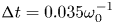 ${\rm \Delta} t=0.035 \omega _0^{-1}$ (
 $0.015\ \textrm {fs}$). The carbon ions are represented by 180 macroparticles per cell, leading to an average number of 720 macroelectrons per cell after ionization. The hydrogen gas and surface layers are modelled by 16 and 450 macroparticles per cell, respectively. Current projection and field interpolation are performed using Esirkepov's (Esirkepov Reference Esirkepov2001) and Sokolov's (Sokolov Reference Sokolov2013) schemes, together with a fourth-order weight factor to quench numerical heating.
The start time of proton acceleration in the foil target depends on the dynamics of the laser-accelerated electrons in the gas layer, and so may vary between simulations. Consequently, the time origin ( $t=0$) is defined henceforth as the moment when the fastest protons from the foil have attained an energy of
 $0.01\ \text {MeV}$.
3. Enhanced ion acceleration in gas–foil targets
3.1. Phenomenology
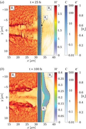
The ion acceleration process taking place in a gas–foil target is illustrated by the two snapshots shown in figure 1. The initial density of the gas layer is  $n_e=0.5\ n_c$, giving rise to maximum proton acceleration from the foil (see below). In each panel are overlaid the density maps of the foil's carbon ions, surface contaminant protons and electrons. Only those electrons originating from the gas are displayed since, as later discussed, those from the foil layer contribute only weakly to the proton final energy. The top panel (figure 1a) shows the early stage of ion acceleration (
 $t=25\ \textrm {fs}$), when the laser pulse has propagated through the undercritical plasma and started interacting with the solid foil. A cloud of fast electrons (light yellow), modulated by the laser ponderomotive force, is breaking out through the rear side of the carbon foil (dark blue). There ensues a (mainly) longitudinal electrostatic field that sets into motion the contaminant protons (cyan). As a result of the laser interaction, a partially electron-depleted channel has formed in the hydrogen gas, with a filament along its axis made of protons and hot (
 ${>}2\ \text {MeV}$) electrons. These electrons are energized by various mechanisms during the laser propagation through the gas, as described in the next section. The high electron energy gain (compared with laser–solid interaction) and the large volume of interaction entail almost complete laser absorption and, therefore, a substantial increase in the electrostatic field set-up at the target rear side.
Ion acceleration in the gas–foil target: 2-D density maps (in  $n_c$ units) of the protons, carbon ions and electrons from the gas layer at two successive times. The dashed lines delineate the boundaries between the three regions
 $R_1,R_2,R_3$ as discussed in § 4. (a) At
 $t=25\ \textrm {fs}$, the
 $3\times 10^{20}\ \textrm {W cm}^{-2}$,
 $30\ \textrm {fs}$ laser pulse coming from the left has traversed the
 $0.5\ n_c$ gas layer, where it has generated a strong current of fast electrons, and hit the solid carbon foil. The thin proton layer starts to be accelerated by the sheath field induced by the fast electrons escaping into vacuum, yet it is still attached to the back side of the foil. (b) At
 $t=100\ \textrm {fs}$, the proton layer has expanded a few microns; its central part has detached from the foil, and its outer front surface has developed a marked concave shape.

Figure 1(b) depicts a later stage of the ion acceleration ( $t=100\ \textrm {fs}$). The transmitted fraction of the laser pulse has then already reflected off the solid foil, and the proton layer, now completely separated on axis from the carbon ions, exhibits a substantial curvature. As the proton layer expands, the outermost (higher-energy) front protons experience a diminishing electric field until reaching saturation in energy.
3.2. Effect of the gas on laser absorption and proton energies
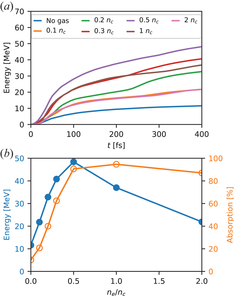
The efficiency of proton acceleration from gas–foil targets closely depends on the electron density of the gas layer. This is illustrated in figure 2(a), which plots the temporal evolution of the maximum proton energy for different gas densities. All curves show a rapid initial rise followed by a slower growth phase. The initial growth rate of the energy tends to increase with the electron gas density up to  $n_e \simeq 0.5\ n_c$, and to decrease with
 $n_e$ beyond this value. The simulations are stopped at
 $t=400\ \textrm {fs}$, that is, when the protons reach the right-hand side of the domain (after travelling a distance of
 ${\sim }31\ \mathrm {\mu }$m) in the optimal
 $n_e=0.5\ n_c$ case. None of the curves has then reached complete saturation; this is a common feature of the reduced 2-D geometry, which causes overestimation of the hot electron density, and hence of the efficiency and time scale of the proton acceleration (Liu et al. Reference Liu, Chen, Zheng, Sheng and Liu2013). A more accurate description would require 3-D simulations, yet currently outside the reach of our computational resources. Despite this limitation, we expect the ordering of the different curves plotted in figure 2 to be representative of the scaling with density that might be obtained in a real-world 3-D scenario.
(a) Temporal evolution of the maximum proton energy for different gas densities. (b) Maximum proton energy at the end ( $t=400\ \textrm {fs}$) of the simulation (blue) and absorbed laser fraction (orange) as a function of gas density.

Hereafter, the maximum proton energy  $\mathcal {E}_{\max }$ is defined as the energy obtained in our simulations at
 $t=400\ \textrm {fs}$. One can see in figure 2 that
 $\mathcal {E}_{\max }$ rises with the electron gas density up to a maximum of
 $\simeq 48\ \text {MeV}$ at
 $n_e=0.5\ n_c$, corresponding to a fourfold increase over the single foil case (
 $n_e=0$), and decreases at higher densities. To understand this behaviour, we plot in figure 2(b) the variations in
 $\mathcal {E}_{\max }$ and the laser absorption coefficient (
 $\mathcal {A}$) with the gas density. Interestingly, the proton energy is found to scale approximately linearly with the laser absorption up to
 $n_e=0.5\ n_c$, where the laser energy is almost fully absorbed. This linear scaling is not obvious since, assuming a one-dimensional (1-D) expansion, the maximum proton energy is expected to evolve as
 $\mathcal {E}_{\max } \propto T_h$ up to a logarithm factor depending on
 $n_h$ and the effective acceleration time (Fuchs et al. Reference Fuchs, Antici, d'Humières, Lefebvre, Borghesi, Brambrink, Cecchetti, Kaluza, Malka and Manclossi2006), while the laser absorption should scale as
 $\mathcal {A} \propto n_h T_h \sim n_e T_h$ (taking
 $n_h \sim n_e$). As the gas density is further increased up to
 $2\ n_c$, the absorption remains nearly saturated while the proton energy is approximately halved.
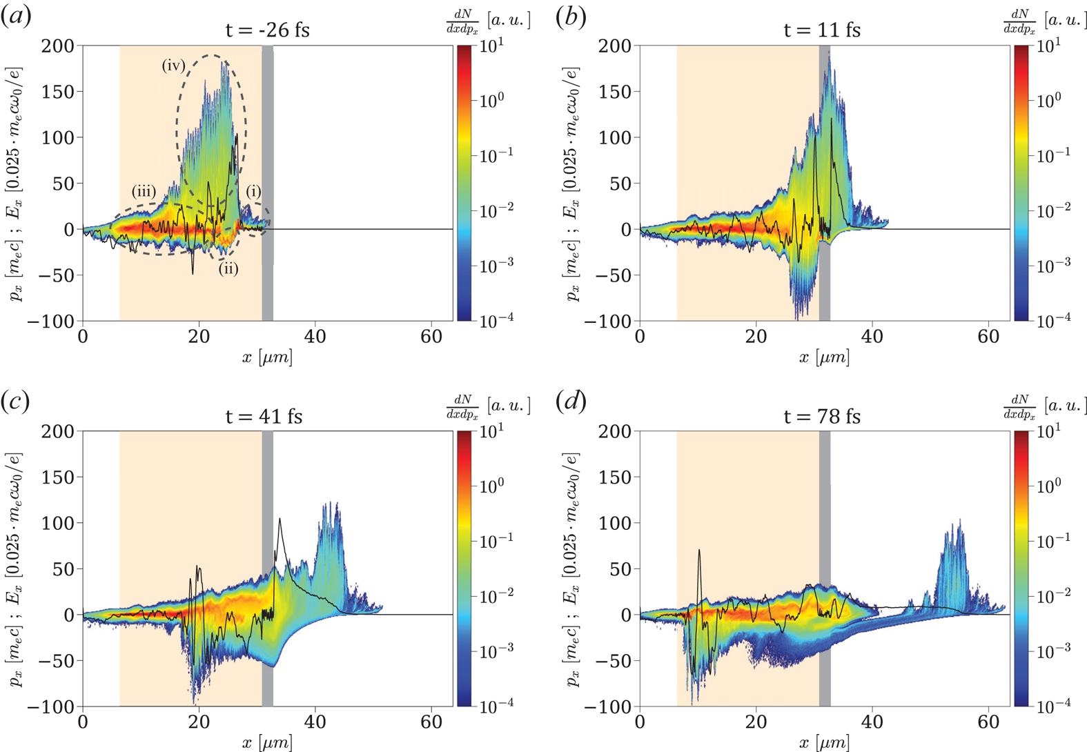
Since the ion acceleration directly results from the dynamics of the high-energy electrons, we display in figure 3(a–d) the longitudinal ( $x-p_x$) phase space of the gas electrons around the laser axis (
 $y=0$) at different times. At
 $t=-26\ \textrm {fs}$ (figure 3a), the laser pulse has traversed the gas, but has not yet reached the foil. Several distinct electron populations can be identified: (i) a bunch of moderately relativistic (
 $0 < p_x/m_ec \lesssim 10$) electrons in the foot of the laser pulse (
 $x\gtrsim 25\ \mathrm {\mu }$m); (ii) a dense and relatively cold, backward-moving (
 $-20\lesssim p_x/m_e c \lesssim 0$) electron flow in the rising part of the laser pulse (
 $22\lesssim x \lesssim 25\ \mathrm {\mu }$m); (iii) a cloud of ‘thermalized’, relativistically hot (
 $\vert p_x \vert /m_e c \lesssim 20$) electrons, travelling in both directions and filling the traversed plasma region; (iv) a spatially modulated cloud of forward-moving, ultra-relativistic (
 $p_x/m_e c \lesssim 180$) electrons located inside the laser pulse (
 $15\lesssim x \lesssim 25\ \mathrm {\mu }$m).
Longitudinal ( $x-p_x$) phase space of the gas electrons (colourmap) and longitudinal electric field
 $E_x$ (black curve) along the laser axis (
 $y=0$) at different times (a–d). The gas and foil layers are shown in light orange and grey, respectively. Different electron groups are highlighted in panel (a).

These electron populations originate from the following sequence of processes.
First, the laser acts as a snowplough when propagating in the gas layer: the electrons accelerated by its ponderomotive force and piled up in its foot make up population (i). As the pulse undergoes erosion during its propagation, its front profile increasingly steepens (Vieira et al. Reference Vieira, Fiúza, Silva, Tzoufras and Mori2010), which enhances the ponderomotive push on the gas electrons (Debayle et al. Reference Debayle, Mollica, Vauzour, Wan, Flacco, Malka, Davoine and Gremillet2017).
The charge imbalance due to the electrons piled up ahead of the pulse induces a strong electrostatic field that pulls them back at high negative momenta, resulting in the backward electron flow (ii). At a lower density, this push–pull mechanism would generate an oscillating plasma wakefield. Here, due to the high plasma density, the highly nonlinear wakefield breaks after just one oscillation, thereby converting its kinetic and potential energy into electron heat via phase mixing (Debayle et al. Reference Debayle, Mollica, Vauzour, Wan, Flacco, Malka, Davoine and Gremillet2017).
Some electrons from this dense thermal reservoir (iii) can be injected into the laser field and driven to ultra-relativistic energies, thus forming population (iv), of same spatial extent as the etched laser pulse. The direct laser acceleration experienced by these electrons is evidenced by their  $\lambda _0/2$ (
 $0.4\ \mathrm {\mu }$m) modulations and their maximum momentum (
 $p_{x,\max }/m_e c \simeq 180$), consistent with the prediction
 $p_{x,\max }/m_e c = a_0^{2}/2$ for a single particle in an electromagnetic plane wave in vacuum. Here account is taken of the intensified laser field (up to
 $a_0 \simeq 20$) due to self-focusing in the gas. The collective interaction of the fast electrons (iv) with the counterstreaming dense flow (ii) contributes to the fast thermalization of the latter (Debayle et al. Reference Debayle, Mollica, Vauzour, Wan, Flacco, Malka, Davoine and Gremillet2017). Note that the coupling between the laser and plasma fields may also trigger resonant-type acceleration mechanisms inside the laser pulse (Pukhov, Sheng & Meyer-ter Vehn Reference Pukhov, Sheng and Meyer-ter Vehn1999; Zhang & Krasheninnikov Reference Zhang and Krasheninnikov2019), which can further boost the maximum electron energies.
All of the above energetic electron populations can contribute to TNSA in the foil target. If the laser pulse is able to propagate through the gas layer and reach the foil, the electrons (i) snowploughed at the laser front are injected into the target, and hence induce the rapid early growth of the rear-side TNSA field (see next Section). In that case, additional MeV-range electrons are generated at the foil's front side through  $J\times B$ heating (Kruer & Estabrook Reference Kruer and Estabrook1985; Debayle et al. Reference Debayle, Sanz, Gremillet and Mima2013), thus reinforcing the early-time TNSA field. Figure 3(b) presents the electron phase space at
 $t=11\ \textrm {fs}$, when the laser pulse is reflecting off the foil while the ultra-relativistic electrons (iv) are breaking out through its back side, hence amplifying the TNSA field (solid black curve). Some of the bunched electrons (i) have been reflected by the TNSA field, making up most of the backward-moving (
 $p_x < 0$) electrons visible at the right of the foil.
At  $t=41\ \textrm {fs}$ (figure 3c), the protons have started expanding from the foil's back side, the fastest ones being located at the peak of the accelerating
 $E_x$ field (
 $x=35\ \mathrm {\mu }$m). The ultra-relativistic electrons have overtaken the proton front and are being decelerated/reflected by the
 $E_x$ field (their maximum longitudinal momentum dropping from
 $p_x/m_e c \simeq 180$ to
 $\simeq 110$ between
 $t=11\ \textrm {fs}$ and
 $t=41\ \textrm {fs}$). A strong
 $E_x$ field is maintained at the ion front by the hot bulk electrons (iii) that have caught up with the expanding ions. The backward-moving (
 $p_x/m_e c \gtrsim -70$) bunch seen at
 $x\simeq 20\ \mathrm {\mu }$m is made of electrons being accelerated and carried away by the reflected laser pulse.
At  $t=78\ \textrm {fs}$ (figure 3d), the non-reflected ultra-relativistic electrons have detached themselves from the thermalized bulk electrons that accompany the accelerating ions. These have then attained a maximum energy of
 ${\sim }25\ \text {MeV}$ and entered their slower acceleration phase (see figure 2a).
The density dependence of the laser absorption revealed by figure 2(b) can be explained using the model proposed in Debayle et al. (Reference Debayle, Mollica, Vauzour, Wan, Flacco, Malka, Davoine and Gremillet2017). The typical mean energy ( $\simeq T_h$) of the thermal bulk electrons was found to be proportional to the electrostatic potential jump across the nonlinear laser-driven wakefield (modified by the ultrarelativistic electron flow). At moderate laser amplitudes (
 $a_0 \lesssim 20$), the thermal electron energy weakly depends on the gas density (see figure 6 of Debayle et al. Reference Debayle, Mollica, Vauzour, Wan, Flacco, Malka, Davoine and Gremillet2017). Specifically, in the range
 $12 \le a_0 \le 20$ of interest in our simulations,
 $T_h$ varies by less than
 $30\,\%$ when the electron density is increased from
 $n_e = 0.1$ to
 $2\ n_c$. Thus, for a fixed gas length, the laser absorption should scale linearly with the gas density, until reaching full absorption when the gas layer is thicker than the laser depletion length. From the model, a 30 fs laser pulse with
 $12 < a_0 < 20$ is expected to be absorbed after propagating
 ${\sim }25\ \mathrm {\mu }$m in a plasma of density
 $n_e=n_c$, and
 ${\sim }50\ \mathrm {\mu }$m in a plasma with
 $n_e = 0.5\ n_c$.
These estimates are consistent with the laser absorption lengths observed in our simulations. For a gas of  $0.5\ n_c$ density and
 $24.5\ \mathrm {\mu }$m length, the laser pulse is still relativistically intense when it hits the foil target, and so the ponderomotively bunched gas electrons and
 $J\times B$ target electrons can trigger an early proton acceleration. At a density
 $n_e=n_c$, by contrast, the laser pulse is strongly weakened when reaching the foil. Although the electron acceleration by the laser field and plasma wave is similar to that observed at
 $n_e=0.5\ n_c$, thus yielding a comparable TNSA field at later times, the absence of the ponderomotively bunched and
 $J\times B$ electrons suppresses the early rise in the TNSA field, which reduces the final proton energy as shown in figure 2(b).
4. Contributions of different plasma regions to the ion-accelerating field
In an electrostatic problem, the electric field at any point in space and time can be calculated as the sum of all electrostatic fields originating from each of the charges in space. Knowing from simulations the spatial distribution of the charge densities, one can calculate the longitudinal electrostatic field arising at  $(x,y,t)$ from some region in space
 $R$ according to the formula
 \begin{equation} E_x(x,y,t)=\frac{1}{2{\rm \pi}}\int_{R}\frac{\rho(x',y',t)(x- x^{\prime})}{(x-x^{\prime})^{2}+(y-y^{\prime})^{2}} \textrm{d}x^{\prime} \textrm{d}y^{\prime},\end{equation}
with  $R$ being the plasma region (an area in 2-D geometry) of interest.
Using (4.1), we investigate the contributions of different plasma regions to the electrostatic field  $E_{x,\rm front}(t)$ induced at the on-axis location of the proton front
 $(x,y)=(x_\textrm {front}(t,0),0)$, where
 $x_\textrm {front}(t,y)$ is the longitudinal position of the outermost (rightmost) protons as a function of time and the transverse coordinate. In practice,
 $x_\textrm {front}(t,y)$ is defined as where the proton density
 $n_p(x,y)$ vanishes with increasing
 $x$.
Three plasma regions ( $R_i$) are considered: (i)
 $R_1$ is the region located to the left of the contaminant proton layer; (ii)
 $R_2$ corresponds to the expanding proton layer; (iii)
 $R_3$ is the region located to the right of the proton layer.
The boundary between  $R_2$ and
 $R_3$ is readily defined as
 $x_{2/3}(y) = x_\textrm {front}(t,y)$. Obviously,
 $R_3$ only contains electrons. Defining the boundary
 $x_{1/2}(y)$ between
 $R_1$ and
 $R_2$ is more complicated as a small fraction of the contaminant protons may initially mingle with the carbon ions and stay inside the carbon plasma at later times. Therefore, looking for the
 $x$ position where
 $n_p(x,y)$ starts to rise from 0 is not relevant if one wishes to locate the main accelerated proton population that can break away from the carbon foil (see figure 1b). Instead, for each transverse position
 $y$, we determine the maximum proton density
 $n_{\max }(y) \equiv \max _x n_p(x,y)$ outside of the area where the carbon ions are present, together with its position,
 $x_{\max }(y)$. The boundary between
 $R_1$ and
 $R_2$ is taken to be the position
 $x_{1/2}(y)$ which is the closest (to the left) to
 $x_{\max }(y)$ and satisfies
 $n_p(x_{1/2}) < n_{\max }/5$. Note that since the leftmost protons of the contaminant layer can be mixed among the carbon ions (this is particularly true far off axis where the proton layer does not completely detach from the foil's back side),
 $R_2$ may comprise a few carbon ions and their accompanying electrons. By contrast,
 $R_1$ includes almost all carbon ions, the gas protons and all of the electrons located at
 $x < x_{1/2}$ (including those filling the gap between the carbon ions and the detached proton layer). The boundaries between the three plasma regions are updated in time, as shown in figure 1(a,b).
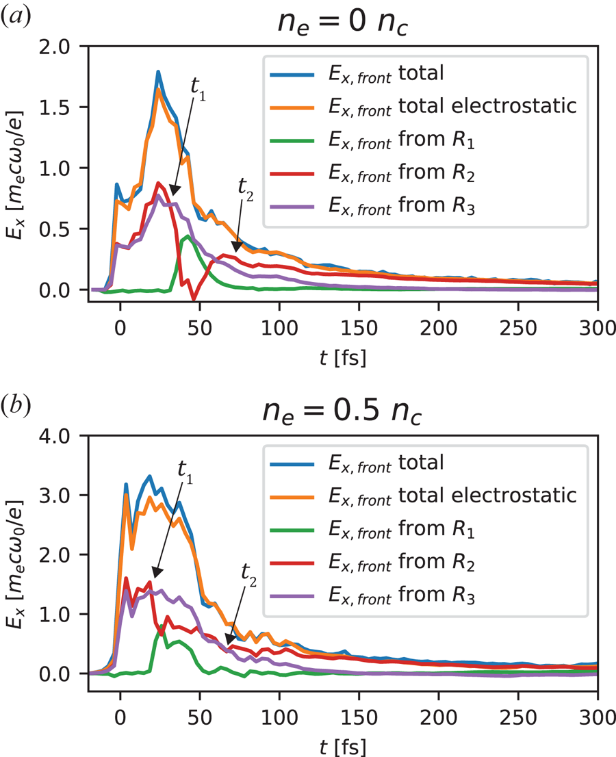
The time evolution of the electrostatic fields generated at the proton front  $x_\textrm {front}(t,0)$ by the three plasma regions is presented in figure 4(a) for the foil target and in figure 4(b) for the gas–foil target with
 $n_e=0.5\ n_c$. Moreover, in order to confirm the validity of the electrostatic approximation, the total electrostatic field (orange curve), obtained by summing up the contributions of the three regions, is compared with the total electric (not just electrostatic) field extracted from the simulation (blue curve). The observed good agreement between the two fields validates the electrostatic approximation, and hence the use of (4.1) to estimate the TNSA field.
Time evolution of the electrostatic fields set-up at the proton front by the plasma regions indicated in figure 1, in the (a) single foil and (b) gas–foil targets. The green, red and purple curves plot the contributions of the charges lying to the left (region  $R_1$), inside (region
 $R_2$) and to the right (region
 $R_3$) of the proton layer, respectively. These fields have been computed using (4.1). The total electrostatic field (orange) is also plotted and compared with the total electric field measured in the simulation. The times
 $t_1$ and
 $t_2$ correspond to the detachment of the proton layer from the foil and the onset of lateral effects, respectively.

Although reaching an  ${\sim }80\,\%$ stronger maximum in the gas–foil target,
 $E_{x,\rm front}(t)$ behaves similarly in both targets. Early in time, the dominant contributions to
 $E_{x,\rm front}$ come from the electrons in
 $R_3$ (purple curve) and the net positive charge contained in
 $R_2$ (red curve). These two regions generate positive (ion-accelerating) electric fields of same amplitude which add up. In other terms, the rightmost (fastest) protons are as much pulled by the sheath electrons in
 $R_3$ as they are pushed by the positively charged proton layer covered by
 $R_2$. This is an expected result in the 1-D geometry that characterizes the initial ion expansion. By contrast, the carbon ions and electrons from
 $R_1$ produce a negligible net field at the proton front. In both targets, the field shows a sudden rise to reach a first peak around
 $t\simeq 0$. As discussed above, it is caused by the arrival of the snowploughed electrons from the gas and the
 $J\times B$ heated electrons from the foil surface.
At  $t=t_1$ (see figure 4a,b), the heated carbon plasma starts to expand, leading to a dense electron sheath permeating the leftmost, lagging part of the proton layer. This transiently reduces the field from
 $R_2$, while, in return, the positive net charge of
 $R_1$ produces a significant accelerating field. This effect, which appears to be most pronounced in the single foil target, ceases when most of the protons have detached from the foil.
At  $t=t_2$ (see figure 4a,b), the on-axis part of the proton layer is well separated from the carbon plasma, so that the fields from
 $R_2$ and
 $R_3$ again mainly account for the total accelerating field. Yet from this time onwards, the push from the positively charged proton layer (
 $R_2$) begins to dominate the fast-decreasing pull from the sheath electrons (
 $R_3$). Actually, the field from the sheath electrons diminishes up to the point of even reaching slightly negative values by
 $t\simeq 150\ \textrm {fs}$. This behaviour results from a multidimensional effect, namely, the transverse curvature of the proton front as evidenced in figure 1(b). The rightmost protons on axis are overtaking most of the off-axis sheath electrons, which end up exerting a decelerating force on those protons. The acceleration of the fastest protons is then solely driven by the repulsive positive charge of the proton layer.
5. Hot-electron contributions to the ion-accelerating field
A closer look at the temporal evolution of the total accelerating field (figure 4) allows one to understand why the gas–foil target performs better than the single foil target. Firstly, the field reaches its absolute maximum much faster and this maximum is also approximately  $1.8\times$ higher. Secondly, the field strength remains close to its peak value during
 ${\sim }50\ \textrm {fs}$, which differs from the rapid post-peak decay observed with the single foil. Since the final proton energy is proportional to the square of the integral of the field curve, the above observations explain the much improved proton acceleration achieved in the gas–foil target (see figure 2).
In the single foil target, the rise time of the accelerating field is consistent with the 30-fs duration of the laser pulse. Its subsequent drop is caused by the plasma expansion and the transverse dilution of the hot electrons. The higher field maximum and subsequent plateau seen in the gas–foil target are due to the successive exits across the foil back side of the distinct hot-electron groups issued from the laser–gas and laser–foil interactions.
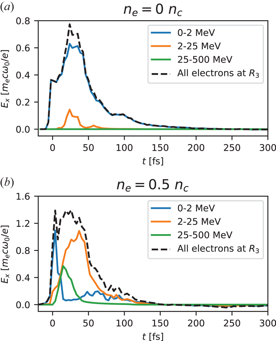
To elucidate these different electron contributions, we divide the electron population lying in region  $R_3$ into three kinetic energy ranges: from zero to approximately the ponderomotive energy (
 ${<}2\ \text {MeV}$), medium energy (
 $2\text {--}25\ \text {MeV}$) and high energy (
 ${>}25\ \text {MeV}$). Again using (4.1), we plot in figure 5 the electrostatic field generated at the proton front by each electron group in the single foil (figure 5a) and gas–foil (figure 5b) targets.
Time evolution of the electric fields generated by different electron groups (see legend) located to the right of the proton front (region  $R_3$) in the (a) single foil and (b) gas–foil targets. The dashed black curve plots the total electric field due to all electrons lying in region
 $R_3$.

With a single foil target (figure 5a), the accelerating field is mainly generated by low-energy electrons ( $<2\ \text {MeV}$), produced by
 $J\times B$ heating (Kruer & Estabrook Reference Kruer and Estabrook1985; Debayle et al. Reference Debayle, Sanz, Gremillet and Mima2013). The electrons in the
 $2\text {--}25\ \text {MeV}$ energy range contribute to only
 ${\sim }10\,\%$ of the field, while the ultra-relativistic (
 $>25\ \text {MeV}$) electrons play a negligible role.
In the gas–foil target (figure 5b), the sheath field results from more diverse electron sources. The  $<2\ \text {MeV}$ electrons snowploughed by the laser in the gas or
 $J\times B$ accelerated at the foil surface are responsible, approximately equally, for the early peak of the sheath field, which lasts for
 ${\sim }15\ \textrm {fs}$. Higher-energy electrons from the gas then take over. The fastest (
 $25\text {--}500\ \text {MeV}$) electrons momentarily account for
 ${\sim }40\,\%$ of the total field, but their contribution rapidly weakens as they move away from the proton front (to a distance
 $r$ larger than their transverse extent, causing the field to decrease as
 ${\sim }1/r$ in two dimensions). Actually, from
 $t \simeq 15\ \textrm {fs}$, most of the field originates from the thermal mid-energy (
 $2\text {--}25\ \text {MeV}$) electrons. As they extend longitudinally throughout the gas–foil target (see figure 3d), they make up a large reservoir of kinetic energy, capable of sustaining a strong sheath field for a (relatively) long time. As they lose energy to the expanding ions, the lower-energy electrons from this population progressively fall into the
 $<2\ \text {MeV}$ group, which leads the associated field to rise again by
 $t\simeq 50\ \textrm {fs}$. Later in time (
 $t\gtrsim 70\ \textrm {fs}$), the
 $<2\ \text {MeV}$ and
 $2\text {--}25\ \text {MeV}$ electron groups turn out to contribute similarly to the sheath field.
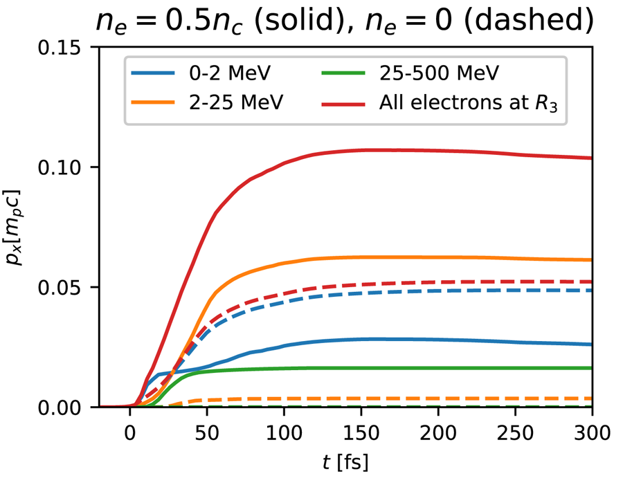
Knowing the temporal evolution of the accelerating fields at the proton front, one can readily calculate the contribution of each electron group within region  $R_3$ to the final proton acceleration. In figure 6 we plot the accumulated proton momentum gain,
 ${p_x(t)=\int _0^{t} eE_{x,\rm front}(t')\, \textrm {d} t'}$, where
 $E_{x,\rm front}(t)$ stands for either the electric field associated with one of the electron groups defined in figure 5, or the total electric field. Owing to the non-additivity of kinetic energies (i.e. the total proton energy differs from the sum of the proton energies resulting from each electron group), we have preferred momentum gains over energy gains to quantify the role of each electron group to TNSA. In the single foil target (dashed curves), as expected, the
 $<2\ \text {MeV}$ electrons overwhelmingly dominate the proton acceleration. In the gas–foil target (solid curves), by contrast, the field that these electrons induce amounts to only
 ${\sim }25\,\%$ of the final proton momentum. The major contribution (
 ${\sim }60\,\%$) is due to
 $2\text {--}25\ \text {MeV}$ electrons, while higher-energy electrons contribute the remaining 15 %. The slight decrease in the total proton momentum seen at
 $t>150\ \textrm {fs}$ results from the total electric field from region
 $R_3$ turning negative – a consequence of the curved proton front, as discussed in § 4.
Time evolution of proton momentum gains from different electron groups (see legend) located to the right of the proton front (region  $R_3$) in the single foil (dashed curves) and gas–foil (solid curves) targets. Momentum gains are calculated by integrating the electric fields plotted in figure 5.

6. Conclusions
Using PIC simulations, we have investigated in detail the processes leading to efficient TNSA in gas–foil targets irradiated by a  $3\times 10^{20}\ \text {W cm}^{-2}$, 30 fs laser pulse. For a fixed gas length of
 ${\sim }25\ \mathrm {\mu }$m, we have found an optimum hydrogen gas density of
 $0.5\ n_c$. These parameters entail an almost complete laser absorption through a combination of electron energization mechanisms involving the laser field and the excited nonlinear plasma waves. Their interplay generates several energetic electron populations which differ by their phase-space properties, each of these populations accounting significantly for proton acceleration in the solid foil.
The main electron contribution to the TNSA field comes from the relativistically hot ( ${\sim }10\ \text {MeV}$) electron bulk resulting from the laser–gas interaction, which generates a strong and relatively long-lived sheath field. The ultra-relativistic gas electrons directly accelerated by the laser field produce a substantial field too, but this field decays quite rapidly as they move away from the foil. The lower-energy (
 $\sim$MeV) electrons snowploughed by the laser in the gas or driven at the foil surface play also a crucial role in building the sheath field at early time and preaccelerate the protons, resulting in an improved overall energy gain. These MeV electrons are efficiently generated only if the laser is intense enough when reaching the foil. The optimal configuration thus corresponds to the case where the laser energy is nearly fully converted into electron kinetic energy inside the gas, but is still able to drive electrons to relativistic energies at the foil surface.
Moreover, this study allowed us, for the first time, to identify as a function of time the plasma regions responsible for the sheath field seen by the fastest protons. This was done by reconstructing, in the electrostatic limit, the electric field at the proton front from the surrounding charge density distributions. At early times, proton acceleration takes place in an essentially 1-D geometry, so that the accelerating field is produced equally by the electrons to the right of the proton front and the net positive charge contained in the proton layer. By contrast, after  ${\sim }70\ \textrm {fs}$, the proton front develops a pronounced curvature due to the transverse proton velocity gradient, which causes the electrons to exert a negligible net force on the outermost protons. The subsequent acceleration of the latter is then mostly sustained by the continuous push exerted by the positively charged proton layer. This new method of analysis of the ion-accelerating field can be readily generalized to other target set-ups.
In our simulations, only the gas density was modified. In general, however, proton acceleration depends on additional parameters such as gas length, foil thickness, laser intensity and duration and on the location of the focal plane. To aid the determination of the optimal gas parameters, which correspond to almost full laser absorption through the gas, one can make use of the scaling given in Debayle et al. (Reference Debayle, Mollica, Vauzour, Wan, Flacco, Malka, Davoine and Gremillet2017).
From a practical standpoint, the proposed plasma density profile could be realized in several ways. In a recent experiment, protons were successfully accelerated from a gas jet coupled to a  $5\ \mathrm {\mu }$m-thick metallic foil (Levy et al. Reference Levy, Bernert, Rehwald, Andriyash, Assenbaum, Kluge, Kroupp, Obst-Huebl, Pausch and Schultze-Makuch2020). While the solid layer resembles that considered in our simulations, the low-density layer was much longer than that simulated (a few
 $100\ \mathrm {\mu}$m versus
 ${\sim }25\ \mathrm {\mu }$m). Employing thinner nozzles and higher gas backing pressures, this experimental scheme has the potential of reaching the range of densities and lengths investigated in the present work. Alternatively, these target parameters could be achieved using carbon nanotube foam coatings, as recently demonstrated in Ma et al. (Reference Ma, Kim, Yu, Choi, Singh, Lee, Sung, Lee, Lin and Liao2019).
To conclude, we have demonstrated that gas–foil targets constitute a promising configuration for TNSA-type proton acceleration under laser interaction conditions available in many university-scale laboratories.
Acknowledgements
D.L. and V.M. were supported by research grants from the Wolfson Foundation and from Dita and Y.L. Bronicki. We acknowledge GENCI for providing us access to the supercomputer Irene under the grants no. A0070506129 and no. A0080507594.
Editor Tünde Fülöp thanks the referees for their advice in evaluating this article.
Declaration of interests
The authors report no conflict of interest.