2. The factor model for the yield to maturity

A celebrated framework that models the yield to maturity is provided by Nelson and Siegel (Reference Nelson and Siegel1987). The framework shows that

(1) \begin{align} ytm(\tau ) = \beta _1 + \beta _2\!\left(\frac{1 - e^{-\lambda \tau }}{\lambda \tau }\right) + \beta _3 \!\left(\frac{1 - e^{-\lambda \tau }}{\lambda \tau } - e^{-\lambda \tau }\right), \end{align}

where $ytm(\tau )$ is the yield to maturity of the bond that will reach maturity after $\tau$ periods, and where $\lambda$ controls the decay rate. $\beta _1$ , $\beta _2$ , and $\beta _3$ are three factors that characterize the shape of the yield curve. A change in $\beta _1$ shifts all the yield to maturity, leading to a shift in the yield curve. Therefore, $\beta _1$ is referred to as the level factor.

The loading on $\beta _2$ is $\frac{1 - e^{-\lambda \tau }}{\lambda \tau }$ , which is a decreasing function of $\tau$ , is close to one for a shortest-term bond and approaches zero for long-term bonds. Therefore, $\beta _2$ impacts the slope of the yield curve, which is normally called the slope factor. Please note that Diebold and Li (Reference Diebold and Li2006) indicated that $\beta _2$ is the negative slope, which is “short minus long”. In other words, a negative $\beta _2$ indicates an upward-sloping yield curve. The last factor $\beta _3$ is associated with a humped shape function $\frac{1 - e^{-\lambda \tau }}{\lambda \tau } - e^{-\lambda \tau }$ . An increase in $\beta _3$ increases the yield curve curvature. It follows that $\beta _3$ is also called the curvature factor. In the end, we can state Equation (1) as follows:

(2) \begin{align} ytm(\tau ) = L + S \!\left(\frac{1 - e^{-\lambda \tau }}{\lambda \tau }\right) + C \!\left(\frac{1 - e^{-\lambda \tau }}{\lambda \tau } - e^{-\lambda \tau }\right), \end{align}

which captures the level - $L$ , slope - $S$ , and curvature - $C$ to model the yield curve. Therefore, we use $L$ , $S$ , and $C$ to denote $\beta _1$ , $\beta _2$ , and $\beta _3$ , respectively. Overall, the Nelson and Siegel (Reference Nelson and Siegel1987) model utilizes these three factors to capture different types of yield curves for empirical analysis and forecasting.

Diebold and Li (Reference Diebold and Li2006) and Diebold et al. (Reference Diebold, Rudebusch and Aruoba2006) extended the Nelson and Siegel (Reference Nelson and Siegel1987) model by showing that the Nelson–Siegel framework could be a latent factor model where $L$ , $S$ , and $C$ are time-varying level, slope, and curvature factors, respectively. They suggest the following state-space representation for the approach:

(3) \begin{align} \begin{bmatrix} L_t - \mu _{L} \\ S_t - \mu _{S} \\ C_t - \mu _{C} \\ \end{bmatrix} = \underbrace{\left[\begin{array}{l@{\quad}l@{\quad}l} a_{11} & a_{12} & a_{13} \\ a_{21} & a_{22} & a_{23} \\ a_{31} & a_{32} & a_{33} \end{array}\right]}_{\boldsymbol{A}} \begin{bmatrix} L_{t-1} - \mu _{L} \\ S_{t-1} - \mu _{S} \\ C_{t-1} - \mu _{C} \end{bmatrix} + \begin{bmatrix} \eta _{L, t} \\ \eta _{S, t} \\ \eta _{C, t} \end{bmatrix} \\[-27pt] \nonumber \end{align}

(4) \begin{align} \begin{bmatrix} ytm(\tau _1) \\ \vdots \\ ytm(\tau _n) \end{bmatrix} = \left[\begin{array}{c@{\quad}c@{\quad}c} 1 & \frac{1 - e^{-\lambda \tau _1}}{\lambda \tau _1} & \frac{1 - e^{-\lambda \tau _1}}{\lambda \tau _1} - e^{-\lambda \tau _1} \\ \vdots & \vdots & \vdots \\ 1 & \frac{1 - e^{-\lambda \tau _n}}{\lambda \tau _n} & \frac{1 - e^{-\lambda \tau _n}}{\lambda \tau _n} - e^{-\lambda \tau _n} \end{array}\right] \begin{bmatrix} L_{t} \\ S_{t} \\ C_{t} \end{bmatrix} + \begin{bmatrix} \epsilon _{\tau _1, t} \\ \vdots \\ \epsilon _{\tau _n, t} \end{bmatrix} \end{align}

Equation (3) is a state equation that includes the unobservable level, slope, and curvature factors. It assumes that the three factors follow an AR(1) process, and $\eta _{j, t}$ where $j \in \left \{ L, S, C\right \}$ is the shock to the state variable $j$ . Equation (4) is called the observation equation. It models the observed yield to maturity and how the three factors determine the yields. $\epsilon _{\tau _i, t}$ where $i \in \left \{ 1, \cdots, n\right \}$ is the measurement error corresponding to the $i$ th yield. The values of $\eta _{j, t}$ and $\epsilon _{\tau _i, t}$ are assumed to be mean zero, normally distributed, independent across time, and independent of each other at time $t$ .

According to Diebold et al. (Reference Diebold, Rudebusch and Aruoba2006), the above state-space model can be estimated based on the Kalman filter and maximum likelihood. They generate optimal filtered and smoothed estimates of the underlying factors. We refer to the above model as our benchmark model, and we extend it following Diebold et al. (Reference Diebold, Rudebusch and Aruoba2006) to study how money supply impacts the shape of the yield curve.

2.1 Data

First, we study how the model captures U.S. treasury securities at different maturity terms. Therefore, we obtained the monthly treasury yields with maturities of 3, 6, 12, 24, 36, 60, 84, 120, 240, and 360 months from the Federal Reserve Economic Data (FRED) for 1993:10 - 2023:09. Overall, we have ten yields over time for the estimation. According to the model based on (3) and (4), there are 29 free parameters, which include $\boldsymbol{A}$ , $\mu _{L}$ , $\mu _{S}$ , $\mu _{C}$ , $\lambda$ , and the covariance matrix in the state equation and observation equation.

Table 1.

Parameter estimate

Note: Sample period, monthly data: 1993:10 - 2023:09. Numbers in parentheses are p-values.

2.2 Estimated factors

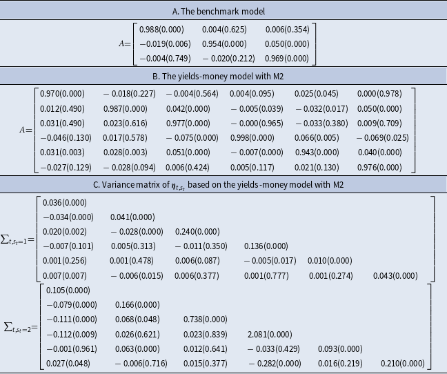
Panel A in Table 1 reports the estimated matrix $\boldsymbol{A}$ , which characterizes the AR(1) process of the factors. The diagonal line in matrix $\boldsymbol{A}$ shows that the dynamics of the three factors are persistent. Their lagged values are highly related to the current values. However, there is not much intertemporal correlation among the different factors. One key output of the benchmark model is the estimated factors. Therefore, we report them in Figure 1. The upper panel in Figure 1 provides the time-varying level factor. We can see the yield curve’s level based on the U.S. treasury security, which had a declining trend before COVID-19. Recently, it has shown an upward trend since 2020. This indicates that the yield curve has shifted upward, and the results are consistent with those of Bauer and Mertens (Reference Bauer and Mertens2022).

Figure 1.

Estimates of level, slope, and curvature factors in the benchmark model. Note: The slope factor is the negative of the yield curve’s slope by construction in the model. We present its absolute value, which captures the slope of the yield curve here.

The middle panel shows the slope factor since 1993. The results are highly consistent with the theory. There were negative valuesFootnote ¹ before and during each shaded recession period. In other words, we find that the inverted yield curve is highly related to recessions and could have reasonable predictive power for recessions. The slope factor particularly suggests an inverted yield curve after 2021, which is consistent with concerns about the state of the financial market. Therefore, there is a considerable risk of an upcoming recession in the next few years. Finally, the lower panel provides the time-varying curvature factor.

3. A regime-switching yields-money factor model

We have shown how the factor model captures the shape of the yield curve in Section 2. In what follows, we would like to revise the model to answer the main research question of this study. We are interested in how the change in the monetary/financial variables, including money supply, is associated with the yield curve. First, the monetary/financial variables could be considered macroeconomic variables that signal the state of the overall economy. Therefore, they are key variables that the financial market participants track. Second, the interaction between monetary variables and the yield curve has been studied in the literature such as Cooper et al. (Reference Cooper, Fuhrer and Olivei2020). Third, monetary assets could be considered substitutes for other financial assets, such as treasury securities. This is because they all provide liquidity services in the modern economy.

To address the above question, we revise the benchmark model following Diebold et al. (Reference Diebold, Rudebusch and Aruoba2006) and Christensen (2015):

(5) \begin{align} \begin{bmatrix} L_t - \mu _{L} \\ S_t - \mu _{S} \\ C_t - \mu _{C} \\ v_{1,t} - \mu _{1} \\ v_{2,t} - \mu _{2} \\ v_{3,t} - \mu _{3} \\ \end{bmatrix} = \underbrace{\left[\begin{array}{l@{\quad}l@{\quad}l@{\quad}l@{\quad}l@{\quad}l} a_{11} & a_{12} & a_{13} & a_{14} & a_{15} & a_{16}\\ a_{21} & a_{22} & a_{23} & a_{24} & a_{25} & a_{26}\\ a_{31} & a_{32} & a_{33} & a_{34} & a_{35} & a_{36}\\ a_{41} & a_{42} & a_{43} & a_{44} & a_{45} & a_{46}\\ a_{51} & a_{52} & a_{53} & a_{54} & a_{55} & a_{56}\\ a_{61} & a_{62} & a_{63} & a_{64} & a_{65} & a_{66} \end{array}\right]}_{\boldsymbol{A}} \begin{bmatrix} L_{t-1} - \mu _{L} \\ S_{t-1} - \mu _{S} \\ C_{t-1} - \mu _{C} \\ v_{1,t-1} - \mu _{1} \\ v_{2,t-1} - \mu _{2} \\ v_{3,t-1} - \mu _{3} \\ \end{bmatrix} + \begin{bmatrix} \eta _{L, z_t, t} \\ \eta _{S, z_t, t} \\ \eta _{C, z_t, t} \\ \eta _{v_1, z_t, t} \\ \eta _{v_2, z_t, t} \\ \eta _{v_3, z_t, t} \\ \end{bmatrix} \end{align}

Equation (5) includes three factors that characterize the shape of the yield curve. There are three more unobservable factors, $v_{1,t}, v_{2,t},$ and $v_{3,t}$ , which correspond to the monetary variables by construction based on the observation equation. The observation equation is

(6) \begin{align} \begin{bmatrix} ytm(\tau _1) \\ \vdots \\ ytm(\tau _n) \\ mg_t \\ ffr_t \\ \pi _t \\ \end{bmatrix} = \left[\begin{array}{c@{\quad}c@{\quad}c@{\quad}c@{\quad}c@{\quad}c} 1 & \frac{1 - e^{-\lambda \tau _1}}{\lambda \tau _1} & \frac{1 - e^{-\lambda \tau _1}}{\lambda \tau _1} - e^{-\lambda \tau _1} & 0 & 0 & 0 \\ \vdots & \vdots & \vdots & 0 & 0 & 0\\ 1 & \frac{1 - e^{-\lambda \tau _n}}{\lambda \tau _n} & \frac{1 - e^{-\lambda \tau _n}}{\lambda \tau _n} - e^{-\lambda \tau _n} & 0 & 0 & 0 \\ 0 & 0 & 0 & 1 & 0 & 0\\ 0 & 0 & 0 & 0 & 1 & 0\\ 0 & 0 & 0 & 0 & 0 & 1\\ \end{array}\right] \begin{bmatrix} L_{t} \\ S_{t} \\ C_{t} \\ v_{1,t} \\ v_{2,t} \\ v_{3,t}\\ \end{bmatrix} + \begin{bmatrix} \epsilon _{\tau _1, t} \\ \vdots \\ \epsilon _{\tau _n, t} \\ 0 \\ 0 \\ 0 \end{bmatrix} \end{align}

Observation equation (6) suggests that the level, slope, and curvature factors sufficiently characterize the shape of the yield curve by placing the “0” restrictions on the parameter matrix. The parameter matrix’s bottom right is a $3\times 3$ identity matrix. This restriction and the assumption of no measurement error for the last three variables in the observation equation link the three monetary variables to the three state variables in the state equation. Note that the state space models (5) and (6) can be compactly presented as follows:

(7) \begin{align} \begin{bmatrix} L_t - \mu _{L} \\ S_t - \mu _{S} \\ C_t - \mu _{C} \\ mg_t - \mu _{mg} \\ ffr_t - \mu _{ffr} \\ \pi _t - \mu _{\pi } \\ \end{bmatrix} = \underbrace{\left[\begin{array}{l@{\quad}l@{\quad}l@{\quad}l@{\quad}l@{\quad}l} a_{11} & a_{12} & a_{13} & a_{14} & a_{15} & a_{16}\\ a_{21} & a_{22} & a_{23} & a_{24} & a_{25} & a_{26}\\ a_{31} & a_{32} & a_{33} & a_{34} & a_{35} & a_{36}\\ a_{41} & a_{42} & a_{43} & a_{44} & a_{45} & a_{46}\\ a_{51} & a_{52} & a_{53} & a_{54} & a_{55} & a_{56}\\ a_{61} & a_{62} & a_{63} & a_{64} & a_{65} & a_{66} \end{array}\right]}_{\boldsymbol{A}} \begin{bmatrix} L_{t-1} - \mu _{L} \\ S_{t-1} - \mu _{S} \\ C_{t-1} - \mu _{C} \\ mg_{t-1} - \mu _{mg} \\ ffr_{t-1} - \mu _{ffr} \\ \pi _{t-1} - \mu _{\pi } \\ \end{bmatrix} + \begin{bmatrix} \eta _{L, z_t, t} \\ \eta _{S, z_t, t} \\ \eta _{C, z_t, t} \\ \eta _{mg, z_t, t} \\ \eta _{ffr, z_t, t} \\ \eta _{\pi, z_t, t} \\ \end{bmatrix} \end{align}

and

(8) \begin{align} \begin{bmatrix} ytm(\tau _1) \\ \vdots \\ ytm(\tau _n) \end{bmatrix} = \left[\begin{array}{c@{\quad}c@{\quad}c} 1 & \frac{1 - e^{-\lambda \tau _1}}{\lambda \tau _1} & \frac{1 - e^{-\lambda \tau _1}}{\lambda \tau _1} - e^{-\lambda \tau _1} \\ \vdots & \vdots & \vdots \\ 1 & \frac{1 - e^{-\lambda \tau _n}}{\lambda \tau _n} & \frac{1 - e^{-\lambda \tau _n}}{\lambda \tau _n} - e^{-\lambda \tau _n} \end{array}\right] \begin{bmatrix} L_{t} \\ S_{t} \\ C_{t} \end{bmatrix} + \begin{bmatrix} \epsilon _{\tau _1, t} \\ \vdots \\ \epsilon _{\tau _n, t} \end{bmatrix} \end{align}

State equation (7) assumes that three monetary variables affect the shape of the yield curve. We mainly consider the money supply growth rate $mg$ , the federal fund rate $ffr$ , and inflation $\pi$ , which impact financial market participants as well as the yield curve. A substantial feature of the model is that we assume that the shocks and their distributions in the state equation depend on an unobserved regime-shift variable, $z_{t}$ , that follows a first-order Markov process governed by the transition matrix

\begin{align*} \mathbf {\Pi }_{t}=\left ( \begin {array} [c]{c@{\quad}c}p_{11} & p_{12}\\ p_{21} & p_{22}\end {array} \right ) \end{align*}

where $p_{ji}=P[z_{t}=j\left \vert z_{t-1}=i\right ]$ , $i,j=1,2$ , and $p_{ji}=1-\sum _{k\neq j}p_{ki}$ is the probability of regime $j$ in period $t$ given that the system was in regime $i$ in period $t-1$ . The states are generic, as in Hamilton (Reference Hamilton1989), and are to be either an expansion or a recession. There can also be other types of high and low states of the economy, given that the states are not observable prior to estimation. Theoretically, the model can be broadened by allowing all the parameters to be regime-dependent. Its current setup assumes that the relationship between variables is stable over time. However, shocks in the system depend on economic regimes. Our assumption regarding the shocks in the state equation aligns with Christensen’s insight (2015). Christensen (2015) studied the period of the zero lower bound (ZLB). The ZLB mainly constrains the variation of short-term yields, whereas medium- and long-term yields can vary significantly. Christensen (2015) then introduced a regime-switching model of the yield curve, assuming the observed state that corresponds to the ZLB. One takeaway is that the short-term yields could be stable during some specific periods, such as the ZLB. On the other hand, the medium- and long-term yields could still vary widely in those periods. Note that the yields determine the yield curve. It follows that the shape of the yield curve is different in terms of economic dynamics. We, therefore, allow the shocks to level, slope, and curvature of the yield curve and the shocks to the monetary variables to be regime-dependent with

(9) \begin{align} \boldsymbol{\eta }_{z_t, t} \in N(\boldsymbol{0}, \boldsymbol{\Sigma }_{z_t}). \end{align}

Please note that these shocks can impact the yield of maturities via the observation equations. It follows that yields are also related to time-varying economic regimes.

Estimating the regime-switching state space model is challenging. The reason is that the predictive density of the state variables is regime-dependent. It follows that the conditional density of the observations depends on the entire sequence of regimes up to time $t$ . The corresponding likelihood function then needs to be integrated over all possible paths, leading to an intractable estimation. Kim (Reference Kim1994) proposed the Kim filter, which provides an approximation of the likelihood function. The Kim filter collapses all possible regimes into finite possible regimes at each filtering recursion by approximation. In doing so, the likelihood function no longer requires the entire sequence of regimes up to time $t$ ; see Kim (Reference Kim1994) and Kim and Kang (Reference Kim and Kang2019) for more details.

To estimate the regime-switching state space model, we consider a variety of measures of money supply, which include the conventional simple-sum M2, Divisia M1 (DM1), DM2, Divisia M3 (DM3), and Divisia M4 minus (DM4M).Footnote ² The M2 series is from the FRED, and the Divisia aggregates are from the Center for Financial Stability. Regarding the interest rate, we obtained the federal fund rates from the FRED and used the Wu and Xia (Reference Wu and Xia2016) shadow federal funds rate for the time period when the federal funds rate hits the zero lower bound. We used the FRED’s annual growth of personal consumption expenditures price index to measure inflation.

Figure 2 gives the estimates of the unobservable factors based on the simple-sum M2 monetary aggregate. We can see that the level factor is lower than the estimate from the benchmark model. The slope factor is relatively consistent between the benchmark and augmented models. The curvature factor based on the simple-sum M2 monetary aggregate is lower than the benchmark estimate. This suggests that the medium-term yield to maturity has declined more over time in the augmented model.

Figure 2.

Estimates of level, slope, and curvature factors for a comparison. Note: The slope factor is the negative of the yield curve’s slope by construction in the model. We present its absolute value, which captures the slope of the yield curve here.

Panel B in Table 1 shows the estimate of matrix $\boldsymbol{A}$ . According to the estimates in Panel B, the level and slope factors are both related to the federal fund rate. An increase in the federal fund rate would increase the level factor, given that $a_{15} = 0.025$ with a $p-$ value of 0.045. This finding is consistent with the theory and practice that an increase in the monetary benchmark rate should encourage a higher cost of borrowing in the financial market. On the other hand, an increase in the federal fund rate would decrease the slope factor, given that $a_{25} = -0.032$ with a $p-$ value of 0.017. This suggests that an increase in the monetary benchmark rate may reduce the short-term treasury security yield more than the yield of long-term treasury security. $a_{24} = -0.005$ with a $p-$ value of 0.039 tells us that an increase in the money supply would also reduce the slope factor. This means that an increase in liquidity would lower the short-term security yield more than a decline in the long-term treasury security. In the end, the inflation change also impacts the slope of the yield curve. Overall, all three monetary variables are important in explaining the yield curve’s slope.

Panel C in Table 1 provides the regime-dependent variance matrix of $\boldsymbol{\eta }_{t, z_t}$ based on the simple-sum M2 monetary aggregate. One can see that the diagonal elements of $\boldsymbol{\Sigma }_{t, z_t=1}$ have lower values than those in $\boldsymbol{\Sigma }_{t, z_t=2}$ . These results indicate that the system has a lower volatility in regime 1. Therefore, we refer to regime 1 as a low-volatility regime, and regime 2 is referred to as a high-volatility regime.

To better understand the two regimes, we calculate and report the filtered probabilities

\begin{align*} p(z_t=i) | \Omega _t, i\in \left \{1, 2\right \}, \end{align*}

where $\Omega _t$ is the information at time $t$ in Figure 3. The high-volatility regime covers major recessions (yellow areas) such as the dot-com bubble, the 2008 financial crisis, and the COVID-19 recession.

Figure 3.

Filtered probabilities of regime 1 (low-volatility regime) and regime 2 (high-volatility regime) based on M2.

The Divisia aggregates are superior measures of money supply since they solve the inconsistency between the theory used to summarize the simple-sum monetary aggregates and economic theory and models in economics studies [see Chrystal and MacDonald (Reference Chrystal and MacDonald1994)]. Therefore, we re-estimate the augmented model with four Divisia aggregates: DM1, DM2, DM3, and DM4M. The estimated level, slope, and curvature factors are reported in Figure 2. They are similar to each other in terms of trend but not in terms of values.

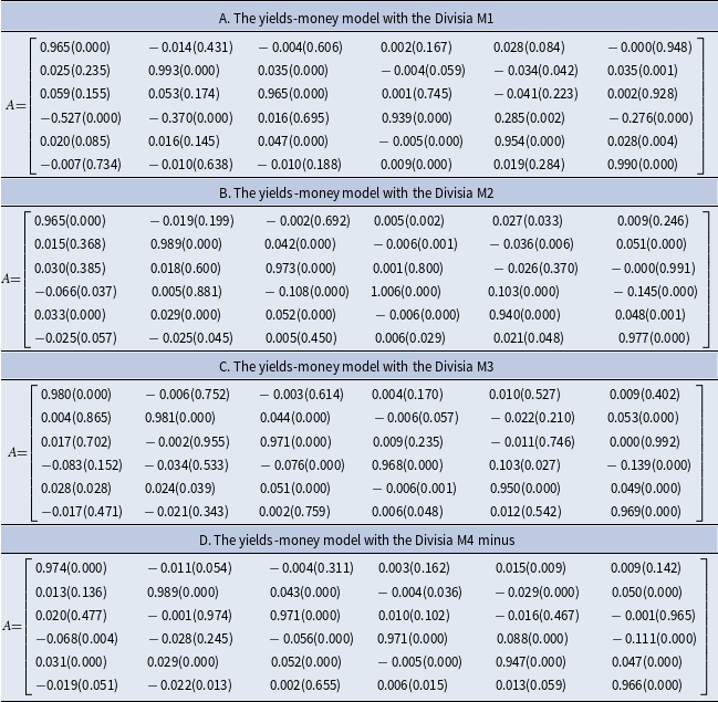
The estimated $\boldsymbol{A}$ matrix is reported in Table 2 for all the Divisia aggregates. Similar to what we discussed above, the slope factor is highly related to changes in the money supply, federal fund rate, and inflation. However, the Divisia aggregates provide more information to explain the yield curve. For example, an increase in DM2 would increase the yield curve level since $a_{14}$ = 0.005 with a $p-$ value of 0.002 in Panel B in Table 2.

Table 2.

Parameter estimate for the transition matrix A based on the divisia aggregates

Note: Sample period, monthly data: 1993:10 - 2023:09. Numbers in parentheses are p-values.

Regarding the filtered probabilities based on the Divisia aggregates, we report all the results in Figure 4. One can see that the high-volatility regimeFootnote ³ covers the major recessions, and this is robust across different measures.

Figure 4.

Filtered probabilities of regime 1 (low-volatility regime) and regime 2 (high-volatility regime) based on the Divisia aggregates.

3.1 Yield curve impulse response functions

To assess the dynamic response of each factor to the change in the money supply, we focus on the state equation (7) to generate the impulse response functions. We are particularly interested in how an increase in the money supply is associated with the level, slope, and curvature of the yield curve. Some recursive ordering of the variables is necessary for identification. A conventional lower triangular identification would assume that the level factor is the most exogenous variable compared with others and that the monetary variables are the least exogenous variable in the state equation. This conventional assumption explicitly holds the belief that changes in the bond market may be driving the monetary variables. We can also reverse the ordering of the variables to assume that the monetary variables drive the bond market. However, there is no clear information about how to rank the variables in the state equation for such identification.

We address this problem by adopting the generalized impulse response function proposed by Pesaran and Shin (Reference Pesaran and Shin1998). According to Pesaran and Shin (Reference Pesaran and Shin1998), the proposed impulse response functions are unique and invariant to the ordering of the variable in the linear system. The response functions are given by

(10) \begin{align} E \left [ v_{t+k}|{\Omega }_{t}, E(\boldsymbol{\eta }_{z_t, t} | \eta _{j, z_t, t} = \delta, z_t ), z_t \right ]-E \left [ v_{t+k}|{\Omega }_{t}, z_t \right ], \end{align}

where ${\Omega }_{t}$ is the information at time $t$ , $\boldsymbol{\eta }_{z_t, t}$ is the vector of shocks in the state equation (7), and $\eta _{j, z_t, t}$ is the shock to the $j$ th variable in the state equation. $v$ is one of three unobservable yield curve factors with $v \in \left \{ L, S, C\right \}$ . According to Pesaran and Shin (Reference Pesaran and Shin1998), equation (10) shocks one variable and integrates the effects of other shocks. Moreover, this class of impulse response functions is invariant to the reordering of the variables, and it takes into account the historical patterns of correlations observed among the different shocks to show the responses.

Given that

\begin{align*} \boldsymbol {\eta }_{z_t, t} \sim N(\boldsymbol {0}, \boldsymbol {\Sigma }_{z_t}) \end{align*}

\begin{align*} \boldsymbol {\Sigma }_{z_t} = \left[\begin {array}{l@{\quad}l@{\quad}l@{\quad}l@{\quad}l@{\quad}l} \sigma _{11, z_t} & \sigma _{12, z_t} & \sigma _{13, z_t} & \sigma _{14, z_t} & \sigma _{15, z_t} & \sigma _{16, z_t}\\ \sigma _{21, z_t} & \sigma _{22, z_t} & \sigma _{23, z_t} & \sigma _{24, z_t} & \sigma _{25, z_t} & \sigma _{26, z_t}\\ \sigma _{31, z_t} & \sigma _{32, z_t} & \sigma _{33, z_t} & \sigma _{34, z_t} & \sigma _{35, z_t} & \sigma _{36, z_t}\\ \sigma _{41, z_t} & \sigma _{42, z_t} & \sigma _{43, z_t} & \sigma _{44, z_t} & \sigma _{45, z_t} & \sigma _{46, z_t}\\ \sigma _{51, z_t} & \sigma _{52, z_t} & \sigma _{53, z_t} & \sigma _{54, z_t} & \sigma _{55, z_t} & \sigma _{56, z_t}\\ \sigma _{61, z_t} & \sigma _{62, z_t} & \sigma _{63, z_t} & \sigma _{64, z_t} & \sigma _{65, z_t} & \sigma _{66, z_t} \end {array}\right]\end{align*}

we have

(11) \begin{align} E(\boldsymbol{\eta }_{z_t, t} | \eta _{j, z_t, t} = \delta, z_t) = (\sigma _{1j, z_t}, \sigma _{1j, z_t}, \sigma _{3j, z_t}, \sigma _{4j, z_t}, \sigma _{5j, z_t}, \sigma _{6j, z_t})'\sigma _{jj, z_t}^{-1}\delta = \boldsymbol{\Sigma }\boldsymbol{e}_j \sigma _{jj, z_t}^{-1}\delta, \end{align}

where $\sigma _{ij, z_t}$ is the element in the variance matrix $\boldsymbol{\Sigma }_{z_t}$ and $\boldsymbol{e}_j$ is the selection vector with unity as its $j$ th element and zeros elsewhere. Note that equation (10) is regime-dependent in the sense that it measures the response of the shape of the yield curve from time $t$ to time $t+k$ to a money supply shock at time $t$ , assuming that the regime is the same from time $t$ to time $t+k$ .

One can see that equation (11) actually allows the shocks with each variable being first in a Cholesky order for the calculation. In other words, the generalized impulse response function calculates the impulse responses for each variable by placing it at the first element in the context of a lower triangular identification. Therefore, the generalized impulse response function reveals how an unexpected change in the money supply suggests the changes in the shape of the yield curve in our model, assuming that the money supply is exogenous in the model. Even though this viewpoint is in line with conventional vertical money supply, we acknowledge that the yield curve and the monetary variables are closely related to economic fundamentals. Therefore, identification is challenging, and a structural interpretation of the shocks is not apparent. Moreover, Sarno and Thornton (Reference Sarno and Thornton2004) showed that zero restrictions are less reasonable under the assumption of efficient markets, and this is a fundamental problem related to the identification of shocks to financial variables in structural VARs. In this context, Moench (Reference Moench2012) used sign restrictions for the identification of a large-scale system of bond yields and 25 macroeconomic variables while treating innovations in the model as nonstructural shocks. Therefore, we follow Moench (Reference Moench2012) and interpret the generalized impulse response functions to understand how different monetary aggregates carry information about future yield curve dynamics.

We then calculate the generalized impulse response functions to show how one standard error shock to the money supply is associated with the dynamics of the level, slope, and curvature factors. The confidence intervals are constructed based on the Markov Chain Monte Carlo algorithms for Metropolis-Hastings. To make a full comparison based on all the money supply measures, we report the responses corresponding to M2, DM1, DM2, DM3, and DM4M in Figures 5, 6, 7, 8, 9.Footnote ⁴

Figure 5.

Impulse responses of the level, slope, and curvature factors to an increase in the money supply (M2). Note: Each panel shows one standard error band.

Figure 6.

Impulse responses of the level, slope, and curvature factors to an increase in the money supply (Divisia M1). Note: Each panel shows one standard error band.

Figure 7.

Impulse responses of the level, slope, and curvature factors to an increase in the money supply (Divisia M2). Note: Each panel shows one standard error band.

Figure 8.

Impulse responses of the level, slope, and curvature factors to an increase in the money supply (Divisia M3). Note: Each panel shows one standard error band.

Figure 9.

Impulse responses of the level, slope, and curvature factors to an increase in the money supply (Divisia M4 minus). Note: Each panel shows one standard error band.

Figure 5 shows the impulse response functions based on the simple-sum M2 aggregate. We find that an increase in the money supply would be associated with a reduction in the level of the yield curve in both regimes. However, these effects are not persistent. Regarding the slope of the yield curve, one can see that a positive shock to the money supply would indicate a reduction in the negative slope, -i.e., “short minus long” in regime 2. In other words, an increase in the money supply implies an increase in the slope of the yield curve in the high-volatility regime, which includes major recessions. Therefore, an increase in the money supply suggests a greater reduction in short-term yields than in long-term yields to restore an upward-sloping yield curve during economic recessions. In the end, the simple-sum M2 monetary aggregate innovations are not accompanied by changes in the yield curve curvature.

Figure 6 provides the impulse response functions based on the DM1 aggregate. One can see that an unexpected increase in the money supply would indicate a decline in the level and the negative slope of the yield curve in the high-volatility regime. Moreover, the positive money supply shock indicates an increase in the curvature of the yield curve in both regimes. It follows that the DM1 aggregate has an important effect on the yield curve during recessions. Figure 7 also confirms that the DM2 aggregate could be associated with the shape of the yield curve in both regimes.

Figure 8 shows the response functions for the DM3 aggregate, which is a broad aggregate. The second row in Figure 8 suggests that an increase in the money supply implies an increase in the slope of the yield curve in both regimes. This effect is short-lived in the low-volatility regime, whereas it is persistent in the high-volatility regime. However, the unexpected changes in the DM3 are less associated with the curvature of the yield curve.

Figure 9 shows the results based on the DM4M aggregate, which is a favored monetary aggregate. In this context, Jadidzadeh and Serletis (Reference Jadidzadeh and Serletis2019) addressed the issue of optimal monetary aggregation in the context of a large demand system. They found that we should use, as a measure of money, the broad Divisia aggregates recommended by Barnett (Reference Barnett and Barnett2016) and Dery and Serletis (Reference Dery and Serletis2021).

Similar to what has been reported previously, an increase in the money supply would announce a decline in the level of the yield curve in both regimes. Moreover, the increase could signal the restoration of an upward-sloping yield curve in the high-volatility regime. A surprising result is that an unexpected increase would imply a reduction in the yield curve slope in the low-volatility regime. The possible reason is that the increase in liquidity would increase the demand for long-term bonds more, leading to a greater reduction in long-term yields in a low-volatility regime. In the end, a positive money supply shock could be associated with medium-term yields, and it decreases the curvature of the yield curve in both regimes. Moreover, this effect is relatively long-lasting in the low-volatility regime.

Overall, the impulse response functions show that the money supply plays an important role in understanding financial markets. An increase in the money supply is likely associated with a downward shift of the yield curve over the business cycle. It also has distinguished implications for the slope and curvature of the yield curve across economic regimes. The favored broad Divisia aggregate could be especially associated with changes in the yield curve’s level, slope, and curvature over the business cycle. Therefore, the Divisia aggregates provide additional information to understand the shape of the yield curve compared with the conventional measure.