






1. Introduction
In recent years, machine learning has proven successful in the classification of both galactic and extragalactic sources (e.g. Bates et al. Reference Bates2012; Lyon et al. Reference Lyon, Stappers, Cooper, Brooke and Knowles2016; Tan et al. Reference Tan, Lyon, Stappers, Cooper, Hessels, Kondratiev, Michilli and Sanidas2018; Liu et al. Reference Liu2019; Karsten et al. Reference Karsten2023; Riggi et al. Reference Riggi2024). For example, Beck et al. (Reference Beck, Szapudi, Flewelling, Holmberg, Magnier and Chambers2021) and (2022) implemented deep neural networks to separate populations of galaxies, quasars, and stars using Pan-STARRS1 optical and WISE IR photometry, achieving galaxy completeness and purity scores of 99.25% and 99.15%. Importantly, many of these machine-learning implementations were not trained on spectroscopic data, but instead relied on published photometric catalogues that often contain
 $\gtrsim10^6$
–
 $10^9$
sources, providing a quick and cheap alternative to classify large, astrophysical populations.
In this paper, we propose and test the viability of a new method to constrain the star formation rate density (SFRD), which uses supervised learning to classify populations of galaxies and quasars using readily available radio continuum and IR catalogues. Since 1.4 GHz radio emission is a reliable tracer of star-formation activity for galaxies whose radio emission isn not dominated by AGN activity, galaxies selected in this manner can be used to investigate the physics of star formation. This allows us to estimate the local (
 $z\lt0.1$
) SFRD using a sample of 11 293 machine-learning selected galaxies and a modified 1.4-GHz SFR calibration that was obtained following the methodology of Molnár et al. (Reference Molnár2021).
This paper is structured as follows. In Section 2, we describe the data used as inputs and labels for the model. In Section 3, we outline the model architecture and training approach, and in Section 4, we assess the performance of the model. In Section 5, we estimate the local SFRD using the 1.4 GHz emission of the
 $z\lt0.1$
depth-matched galaxy sample, and correct this result for completeness in Section 6. We discuss the efficacy and the limitations of the method in Section 7 and conclude in Section 8. Throughout the paper, we adopt a
 $\Lambda$
cold dark matter (
 $\Lambda$
CDM) cosmology with
 $\Omega_M=0.27$
,
 $\Omega_{\Lambda}=0.73$
,
 $\Omega_K=0$
, and
 $H_0=73 \rm \;km\,s^{-1} \,Mpc^{-1}$
.
2. Datasets
2.1. RACS-mid
The Australian Square Kilometre Array Pathfinder (ASKAP, Hotan et al. Reference Hotan2021) has surveyed
 ${\sim}90\%$
of the sky as part of the Rapid ASKAP Continuum Survey (RACS, McConnell et al. Reference McConnell2020), with the aim of providing a sky model for the calibration and validation of future ASKAP surveys. RACS commenced in 2019 and observed each area of the sky with a
 ${\sim}$
15-min integration time, achieving a root-mean-square noise of
 ${\sim}200-260\,\unicode{x03BC}\,{\rm Jy}\,{\rm PSF}^{-1}$
and a resolution of
 ${\sim}$
8–15 arcsec. RACS consisted of three major observing epochs, RACS-low (McConnell et al. Reference McConnell2020; Hale et al. Reference Hale2021), RACS-mid (Duchesne et al. Reference Duchesne2024), and RACS-high (Duchesne et al. Reference Duchesne2025), centred on effective frequencies of 887.5, 1 367.5, and 1 655.5 MHz, respectively.
Since radio continuum emission has the potential to trace SFRs without significant dust extinction (Gordon et al. Reference Gordon2004; Osterbrock Reference Osterbrock1989; Bowler et al. Reference Bowler2015), tabular data from the RACS-mid catalogue are used as features for the binary-classification model implemented in this paper. The second data release of RACS-mid (Duchesne et al. Reference Duchesne2024) contains 1 493 sky images at 1 367.5 MHz with a bandwidth of 144 MHz. These images were convolved to a common resolution and mosaicked, yielding a series of near constant sensitivity images that cover the sky up to a declination of
 $+49^{\circ}$
. Accompanying these images are source and component catalogues, consisting of 3105 668 radio sources with an estimated completeness of 95% above 2 mJy (Duchesne et al. Reference Duchesne2024).
The source catalogue was accessed through the Common wealth Scientific and Industrial Research Organisation (CSIRO) ASKAP Science Data Archive.Footnote a Source features in the catalogue include the peak and total flux densities; the position angle and major and minor axes of the source, the deconvolved source, and the full width at half maximum of the PSF of the field; the number of Gaussian components of the source and the source structure code (single or multiple Gaussians); and the source type flag (resolved, unresolved, or spurious).
2.2. WISE All-Sky
NASA’s Wide-Field Infrared Survey Explorer (WISE, Wright et al. Reference Wright2010) imaged the full infrared sky across four pass bands centred at 3.4, 4.6, 12, and 22
 $\unicode{x03BC}$
m (W1, W2, W3, W4), achieving 5
 $\sigma$
point source sensitivities greater than 0.08, 0.11, 1, and 6 mJy respectively in uncrowded regions. Following the depletion of its coolant, WISE continued mapping the sky in the W1 and W2 passbands with the aim of detecting near-Earth moving objects including asteroids and comets, as the Near-Earth Object Wide-field Infrared Survey Explorer (NEOWISE, Mainzer et al. 2011, 2014) until the mission ended in 2024.
The WISE All-Sky Catalogue (Cutri & et al. Reference Cutri2012) contains IR photometry and astrometry for over 300 million sources, and was combined with data collected during NEOWISE to produce the AllWISE catalogue (Cutri et al. Reference Cutri2021), which includes
 ${\sim}750$
million sources and improved sensitivity in the W1 and W2 bands. unWISE is the most recent and complete release of WISE and NEOWISE data, with
 ${\sim}2$
billion sources thanks to deeper imaging and improved modelling of crowded regions (Schlafly et al. Reference Schlafly, Meisner and Green2019). However, in line with the model and data used by Beck et al. (Reference Beck, Dodds and Szapudi2022), data fields from the WISE All-Sky Catalogue are used as inputs for the binary-classifier model. The source catalogue was accessed via the NASA/IPAC Infrared Science Archive (IRSA).Footnote
b
2.3. WISE-PS1-STRM
The WISE
 $\times$
PanSTARRS1 Source Types and Redshifts with Machine learning (WISE-PS1-STRM, Beck et al. Reference Beck, Dodds and Szapudi2022) catalogue contains source classifications and photometric redshifts for 354 590 570 objects. Building on an earlier catalogue that classified PanSTARRS1 3
 $\pi$
Data-Release 1 (PS1 3
 $\pi$
DR1, Chambers et al. Reference Chambers2016; Flewelling et al. Reference Flewelling2020) sources using supervised learning (PS1-STRM, Beck et al. Reference Beck, Szapudi, Flewelling, Holmberg, Magnier and Chambers2021), the WISE-PS1-STRM catalogue was constructed by cross-matching WISE All-Sky and PS1
 $3\pi$
DR2 sources. The cross-matched objects were then classified into galaxies, quasars, and stars using a deep neural network, with the inclusion of WISE IR colours achieving greater star sample purity and quasar sample completeness compared to the earlier model which relied on optical PS1 observations alone.
The training set for the Beck et al. (Reference Beck, Dodds and Szapudi2022) machine learning algorithm consisted of matched spectroscopic observations, mainly from the 14th data release of the Sloan Digital Sky Survey (SDSS DR14 Abolfathi et al. Reference Abolfathi2018), but supplemented by spectra from the fourth data release of the DEEP2 Redshift Survey (Newman et al. Reference Newman2013), the VIMOS Public Extragalactic Redshift Survey (VIPERS) public data release 2 (VIPERS PDR-2, Scodeggio et al. Reference Scodeggio2018), the WiggleZ Dark Energy Survey (Drinkwater et al. Reference Drinkwater2018), the 3rd data release of zCOSMOS (Lilly et al. Reference Lilly2009), and the VIMOS VLT Deep Survey (VVDS, Le Fèvre et al. Reference Le Fèvre2013). A separate deep neural net was then used to estimate photometric redshifts for those objects they classified as galaxies.
For the supervised-learning model implemented in this paper, the source classifications from WISE-PS1-STRM are used to label the training data set of cross-matched RACS-mid and WISE All-Sky sources. WISE-PS1-STRM data was accessed via Mikulski Archive for Space Telescopes (MAST) CasJobs.Footnote c
3. Supervised-learning algorithm implementation
This section describes the datasets and algorithms that were used to train a simple binary classification model to predict the natures of the RACS-mid sources using the galaxy and quasar labels from Beck et al. (Reference Beck, Dodds and Szapudi2022). These model predictions are then used to select an uncontaminated sample of star-forming galaxies (SFGs) that enable the local SFRD to be estimated in Section 7.
3.1. Our dataset
To obtain the data and labels for the binary-classifier model, the RACS-mid catalogue from Duchesne et al. (Reference Duchesne2024) was cross-matched with the WISE-PS1-STRM catalogue from Beck et al. (Reference Beck, Dodds and Szapudi2022) using TOPCAT version 4.10-2Footnote d (Taylor Reference Taylor2005). The cross-match was performed using the sky algorithm with a maximum error of 1.5 arcsec, ensuring that no row from either table appeared more than once in the final table, yielding an initial cross-match sample consisting of 426 815 sources. Any sources that were classified as stars or were listed as unsure in the Beck et al. (Reference Beck, Dodds and Szapudi2022) catalogue were then dropped. The final cross-match sample consisted of 389 392 sources, of which 14.2% were quasars and 85.8% were galaxies.
3.2. Our model
To classify the final cross-matched sample into galaxies and quasars, a gradient-boosted decision tree model from the XGBoost package (Chen & Guestrin Reference Chen and Guestrin2016) was implemented. Here, we describe our approach for this model.
3.2.1. Input features
The same WISE features used by Beck et al. (Reference Beck, Dodds and Szapudi2022) were selected as model inputs. These included the profile-fit photometry and uncertainties in the four WISE passbands for different aperture sizes, as well as features relating to the observation quality. In total, this amounted to 68 WISE features.
For the RACS-mid data, all features that related to the source properties and the associated uncertainties were selected as model inputs, amounting to 28 features in total. These included the peak and total fluxes, extended sources flags, and features relating to the source size and extent. Details on the RACS and WISE features used as model inputs can be found in Table A1 in Appendix A.1.
Any qualitative features were assigned numerical values, and features with information relating to multiple bands were split into separate inputs, yielding 105 features in total. Details on this process can be found in Appendix A.2.
3.2.2. Training approach
To optimise and assess the performance of the binary-classifier model, the cross-matched sample was split into three sets for training, validation, and testing, each making up 70%, 15%, and 15% of the total sample, respectively. These splits were performed using StratifiedShuffleSplit from the Scikit-learn package (Pedregosa et al. Reference Pedregosa2011) to maintain the class representation of galaxies and quasars across each of the three groups.
Given the significant class imbalance of the cross-matched sample (
 ${\sim}$
85% galaxies and
 ${\sim}$
15% quasars), the effects of various under- and over-sampling techniques were trialled using the imblearn package (Lemaître et al. Reference Lemaître, Nogueira and Aridas2017). Resampling techniques that were tested included random oversampling (RandomOverSampler), random undersampling (RandomUnderSampler), oversampling using the Synthetic Minority Over-sampling Technique (SMOTE, Chawla et al. Reference Chawla, Bowyer, Hall and Kegelmeyer2002), cleaning using Tomek links (Tomek, Tomek Reference Tomek1976), and a combination of both SMOTE and Tomek links (SMOTETomek, Batista et al. Reference Batista, Bazzan and Monard2003). Each of these resampling methods resulted in an even class distribution between galaxies and quasars, allowing the model to more effectively learn the patterns in the data.
To save on computation time, a smaller training and validation set were used to assess the performance of the different resampling techniques prior to extending the pipeline to the full sample. This smaller data set consisted of cross-matched sources with
 $25^\circ \lt \delta \lt 50^\circ$
, amounting to 58 389 sources, of which 49 452 were galaxies and 8 937 were quasars. 70% of these sources were allocated for model training, while the remaining 30% formed the test set. Note that these resampling methods were applied to the training data set only to avoid data leakage.
For each resampling method, the mean F1 score across five cross-validation folds was calculated. Based on this, random oversampling of the minority class was found to achieve the best performance on the trial dataset. The same pipeline was therefore extended to the full, final cross-matched sample, consisting of 389 392 objects, of which
 ${\sim}86\%$
were galaxies and
 ${\sim}14\%$
were quasars. After oversampling, an even split was achieved between the two classes in the training set. Details of the final sample distribution between galaxies and quasars can be found in Table 1. The performance of this final model is discussed in Section 4.
Hyperparameters were optimised using Randomized SearchCV and Hyperopt following the process described in Appendix A.3, and early_stopping_rounds was set to 100 to avoid overfitting. The optimised model hyperparameters are listed in Table A2.
The class distribution for the final training, validation and test datasets, including the contribution from real and synthetic sources after random oversampling of the quasar class.

Table 1. Long description
The table shows the distribution of real and synthetic galaxies and quasars across training, validation, and testing datasets. It has six rows and four columns. The columns are labeled Sample, Training, Validation, and Testing. The rows are labeled Real galaxies, Real quasars, Synthetic galaxies, Synthetic quasars, Fraction galaxies, and Fraction quasars. Row 1: Real galaxies, Training: 233 743, Validation: 50 088, Testing: 50 088. Row 2: Real quasars, Training: 38 831, Validation: 8 321, Testing: 8 321. Row 3: Synthetic galaxies, Training: 0, Validation: 0, Testing: 0. Row 4: Synthetic quasars, Training: 194 912, Validation: 0, Testing: 0. Row 5: Fraction galaxies, Training: 0.50, Validation: 0.86, Testing: 0.86. Row 6: Fraction quasars, Training: 0.50, Validation: 0.14, Testing: 0.14.
4. Classification results
The final model performance was evaluated using the test data set and a series of metrics including accuracy, precision, recall, the F1 score, the cross-entropy, the area under the receiver operating characteristic curve (ROC AUC), and the area under the precision-recall curve (AUPRC). The metric values for the optimised model are provided in Table 2 and the confusion matrix for the model predictions on the full dataset is shown in Figure 1.
Performance metrics for the optimised XGBClassifier model with random oversampling of the quasar class.

Table 2. Long description
A table with two columns labeled Metric and Value, and nine rows. The table compares various performance metrics for an optimized XGBClassifier model with random oversampling of the quasar class. Row 1: Metric, Accuracy; Value, 0.94. Row 2: Metric, Weighted F1 score; Value, 0.93. Row 3: Metric, Quasar precision; Value, 0.80. Row 4: Metric, Quasar recall; Value, 0.73. Row 5: Metric, Quasar F1 score; Value, 0.76. Row 6: Metric, Galaxy precision; Value, 0.96. Row 7: Metric, Galaxy recall; Value, 0.97. Row 8: Metric, Galaxy F1 score; Value, 0.96. Row 9: Metric, Cross-entropy; Value, 0.16. Row 10: Metric, ROC AUC; Value, 0.97. Row 11: Metric, AUPRC; Value, 0.99.
Confusion matrix for the model predictions for all 389 392 sources in the cross-matched dataset.

Model predictions were generated for the entire final cross-matched sample. Of the 389 392 sources, the model predicted that 336 674 are galaxies and 52 718 are quasars, making up
 ${\sim}86\%$
and 14% of the sample, respectively.
To provide an independent constraint on the AGN contamination fraction of the model-selected galaxy sample, we cross-matched those sources identified by the model as galaxies with the Milliquas catalogue (Flesch Reference Flesch2023). This process identified 7712 AGN in our galaxy sample of the 152 060 galaxies in the overlapping region between the two catalogues. This corresponds to an AGN contamination fraction of 0.05 across all redshifts, or 0.03 for the subset of sources with
 $z\lt0.1$
.
5. Estimating the SFRs of the model-selected galaxy sample
5.1. Radio and total infrared luminosities of the galaxy sample
Having identified a population of galaxies using the optimised model, it is possible to estimate the SFRs using their 1.4 GHz radio-continuum emission, since the emission in this band is a reliable tracer of star formation that does not suffer significantly due to dust extinction (Osterbrock Reference Osterbrock1989; Gordon et al. Reference Gordon2004; Bowler et al. Reference Bowler2015; Molnár et al. Reference Molnár2021). This and Section 5.2 below follow the methodology presented in Molnár et al. (Reference Molnár2021) to determine a modified 1.4-GHz SFR prescription for a sample of galaxies in a given redshift range. Note that since we use the predicted galaxy redshifts from Beck et al. (Reference Beck, Szapudi, Flewelling, Holmberg, Magnier and Chambers2021), our luminosity and SFRD calculation below is limited to their galaxy sample. However, we do not include those galaxies that were missed by our model and classified as quasars.
The luminosity at frequency
 $\nu$
is given by:
 \begin{align}\bigg( \frac{L_{\nu}}{{\rm W} \,{\rm Hz}^{-1}} \bigg) = (9.52 \times 10^{15}) \times 4\pi \times K(z) \times \bigg(\frac{D_L}{\rm Mpc} \bigg)^2 \bigg( \frac{S_{\rm int}^{\nu}}{\rm mJy}\bigg),\end{align}
where
 $9.52 \times 10^{15}$
is the conversion factor from
 $\rm Mpc^2 \, mJy$
to
 $\rm W\,Hz^{-1}$
,
 $D_L$
is the luminosity distance to the source, and
 $S_{\rm int}^{\nu}$
is the measured flux density at frequency
 $\nu$
. The k-correction factor
 $K(z) = (1 + z)^{-(1 + \alpha)}$
accounts for redshift-related effects and depends on the spectral index,
 $\alpha$
, defined as
 $S_{\rm int} \propto \nu^{\alpha}$
. To calculate the 1.4-GHz radio luminosity, a radio spectral index of
 $-0.7$
is assumed, as is standard for SFGs at 1.4 GHz (Kimball & Ivezić Reference Kimball and Ivezić2008; Molnár et al. Reference Molnár2021). Note that
 $S_{\rm int}$
is measured at 1 367.5 MHz for RACS-mid, however it was treated as equivalent to the 1.4 GHz integrated flux density for the purposes of this study.
To calculate the total IR (TIR) luminosity, the observed WISE Vega magnitudes,
 $m_{{\rm vega}, x}$
, are first converted to integrated flux densities,
 $S_{\rm int}^{Wx}$
, via:
 \begin{equation}S_{\rm int}^{Wx} = S_{0, x} \times 10^{\frac{-m_{{\rm vega}, x}}{2.5}},\end{equation}
where x represents the WISE band number, and
 $S_{0,x }$
is the zero magnitude flux density in the given band, with values of 390.54, 171.787, 31.674, and 8.363 for bands W1, W2, W3, and W4, respectively (Wright et al. Reference Wright2010; Jarrett et al. Reference Jarrett2011).
Next, the methodology presented in Grundy et al. (Reference Grundy2023) that is based on Cluver et al. (Reference Cluver, Jarrett, Dale, Smith, August and Brown2017) is followed to determine the TIR luminosity. For SFGs, the WISE W3 band contains a significant contribution from the ISM, in addition to emission from evolved stellar populations. The ISM contribution arises from a variety of sources, but notably from polycyclic aromatic hydrocarbon (PAHs), which have been shown to trace regions of active star formation without suffering from dust-extinction biases (Houck et al. Reference Houck, Weedman, Le Floc’h and Hao2007; Alonso-Herrero et al. Reference Alonso-Herrero2014; Shipley et al. Reference Shipley, Papovich, Rieke, Brown and Moustakas2016; Kim et al. Reference Kim2024; Ronayne et al. Reference Ronayne2024). To remove the stellar contribution from the W3 band integrated flux, it is assumed as in Helou et al. (Reference Helou2004), Cluver et al. (Reference Cluver, Jarrett, Dale, Smith, August and Brown2017), and Grundy et al. (Reference Grundy2023), that the near-infrared W1 band is a proxy for the stellar emission, and that 15.8% of the W1 band stellar emission is also detected in the W3 band. Therefore, the W3PAH integrated flux component is obtained by subtracting 15.8% of the W1 band flux from the W3 band flux. The W3PAH luminosity,
 $L_{\rm W3PAH}$
, is then calculated using Equation (1) above, assuming a flat (
 $\alpha = 0$
) IR spectrum for the k-correction factor (Wright et al. Reference Wright2010; Jarrett et al. Reference Jarrett2011; Izotova & Izotov Reference Izotova and Izotov2019).
The TIR luminosity is finally obtained according to the relationship presented in Cluver et al. (Reference Cluver, Jarrett, Dale, Smith, August and Brown2017):
 \begin{align} \log\bigg( \frac{L_{\rm TIR}}{L_{\odot}} \bigg) &= (0.889 \pm 0.018) \, \log \bigg( \frac{\nu L_{\rm W3PAH}}{L_{\odot}} \bigg) \nonumber\\ &\quad+ (2.21 \pm 0.15),\end{align}
where
 $\nu$
is the W3 band central frequency (
 $2.498 \times 10^{13}$
Hz, Wright et al. Reference Wright2010).
Figure 2 shows the Infrared-Radio Correlation (IRRC, 1.4 GHz vs. TIR luminosities) for the model-selected galaxy sample in different redshift bins. On a log-log scale, the slope of the best-fit linear model of the form
 $\log({L}_{1.4 \,{\rm GHz}}) = m\,\log(L_{\rm TIR}) +c$
indicates whether the IRRC is linear (
 $m=1$
) or non-linear (
 $m\ne1$
) across a given redshift range. In each panel of Figure 2, the colour bar indicates the logarithm of the number of sources in each pixel, and the dashed blue line is the best-fit model (
 $m=1.114 \pm 0.009$
,
 $c=10.2 \pm0.1$
) for the depth-matched,
 $z\lt0.2$
galaxy sample from Molnár et al. (Reference Molnár2021). The black line shows the best-fit linear model to each data set, which was obtained using the curve_fit command from the scipy.optimize package (Virtanen et al. Reference Virtanen2020). The
 $1\sigma$
uncertainties in the linear-fit parameters were calculated using a bootstrapping technique, whereby the data points were resampled with replacement and a new linear fit was calculated for each iteration. The reported uncertainties are the standard deviations of the individual slopes and intercepts across 1 000 iterations of resampling.
The 1.4 GHz vs. TIR luminosities for the model-selected galaxy sample across different redshift bins. The colour map indicates the logarithm of the number of sources in each pixel and the contours show the 10th, 50th, and 90th percentiles. For each graph, the redshift range and the number of sources is specified in the top left corner. The best-fit linear trend for each graph is shown in black, while the dashed blue line shows the relationship from Table 5 of Molnár et al. (Reference Molnár2021). For both, the shaded region indicates the associated
 $1\sigma$
confidence interval. The bottom-right panel shows the results for the full dataset.

Figure 2. Long description
Nine scatter plots depict the relationship between 1.4 GHz and TIR luminosities for a galaxy sample across different redshift bins. Each plot shows the logarithm of the number of sources in each pixel and the contours indicating the 10th, 50th, and 90th percentiles. The redshift range and the number of sources are specified in the top left corner of each plot. The best-fit linear trend for each plot is shown in black, while the dashed blue line shows the relationship from Table 5 of Molnar et al. (2021). The shaded region indicates the associated confidence interval. The bottom-right plot shows the results for the full dataset. Panel A: 0 <= z < 0.05, N = 7176. Panel B: 0.05 <= z < 0.1, N = 9765. Panel C: 0.1 <= z < 0.15, N = 8064. Panel D: 0.15 <= z < 0.2, N = 8232. Panel E: 0.2 <= z < 0.4, N = 36462. Panel F: 0.4 <= z < 0.6, N = 42705. Panel G: 0.6 <= z < 0.8, N = 48593. Panel H: all z, N = 213490.
Figure 2 shows that the IRRC for the model-selected galaxy sample is not consistent with that of Molnár et al. (Reference Molnár2021) across any redshift range. When all data is included, as in the bottom-right panel of Figure 2, the slope of the IRRC is consistent with that of Molnár et al. (Reference Molnár2021), but there is a vertical shift of
 ${\sim}1.2$
. However, at lower redshifts, the fits are vastly different to Molnár et al. (Reference Molnár2021). For
 $z\lt0.1$
, the fits deviate due to the presence of a subsample of galaxies with higher radio luminosities and lower TIR luminosities, which flatten the slope of the best-fit model. As z increases, the dataset suffers from Malmquist bias, with a dearth of sources with
 $\log(L_{1.4 \, {\rm GHz}}) \lesssim22$
, indicating the sample is incomplete beyond
 $z\sim0.05$
–
 $0.1$
due to the shallowness of RACS-mid. This is consistent with Figure 3, which shows that these high-luminosity sources also have higher mean redshifts.
To account for these effects, the RACS-mid and WISE catalogues were depth-matched as in Molnár et al. (Reference Molnár2021), using the process described in Section 5.2 below. In addition, the higher-completeness, low-z population is considered separately for the calculation of the cosmic SFRD in Section 7.
Description and sizes of the different samples referred to in this study at each stage of the classification and cleaning process.

Table 3. Long description
The table has 10 rows and 3 columns. The columns are labeled Sample name, Description, and Size. Row 1: Initial cross-match, The sample obtained by cross-matching, 426 815. Row 2: Sample, WISE-PS1-STRM with RACS-mid, ~6% unsure, ~3% stars. Row 3: Final cross-match, The initial cross-match sample after removing sources, 389 392. Row 4: Sample, listed as stars or unsure in WISE-PS1-STRM, (86% galaxies, 14% quasars). Row 5: Model-selected galaxy, The sources from the cross-match sample after star, 336 674. Row 6: Sample, removal classified as galaxies by the model. Row 7: Model-selected quasar, The sources from the cross-match sample after star, 52 718. Row 8: Sample, removal classified as quasars by the model. Row 9: Model-selected galaxy, Sources in the galaxy sample with a S/N, 213 490. Row 10: Sample (S/N cut), The remaining galaxies from the galaxy sample, 13 325. Row 11: Depth-matched galaxy, (S/N cut) after being corrected for the different, 11 293. Row 12: Galaxy sample, sensitivities of the WISE and RACS-mid surveys, depth-matched. Row 13: The low-redshift depth-matched galaxy sample.
Similar to Figure 2 but with a colour map showing the logarithm of the mean redshift in each pixel.

5.2. Depth-matching the radio and infrared catalogues
First, to reduce noise in the dataset, an initial signal-to-noise cut was made on the model-selected galaxy sample, removing any sources with S/N
 $\lt5\sigma$
. This reduced the sample size to 213 490 sources.
Then, to correct for the different sensitivities of the WISE and RACS-mid catalogues, the model-selected galaxy sample was cleaned to ensure both surveys probe equivalent depths, following Sargent et al. (Reference Sargent2010) and Molnár et al. (Reference Molnár2021). To do this, the luminosity corresponding to the
 $5\sigma$
flux-density limit of the RACS-mid catalogue (1.6 mJy, Duchesne et al. Reference Duchesne2024) was calculated using Equation (1) at the redshift associated with each galaxy.
Next, to convert the 1.4 GHz radio luminosities to their corresponding TIR luminosities, the median q parameter of 2.54 from Molnár et al. (Reference Molnár2021) was used. The parameter q is often used to characterise the IRRC (Helou et al. Reference Helou, Soifer and Rowan-Robinson1985), and relates the TIR and radio luminosities to each other via:
 \begin{equation} q_{\rm TIR} = \log \bigg( \frac{L_{\rm TIR}}{3.75 \times 10^{12}\,{\rm W}}\bigg) - \log \bigg( \frac{L_{\rm 1.4 \, GHz}}{\rm W\, Hz^{-1}}\bigg) .\end{equation}
Finally, Equations (3) and (1) were inverted to determine the W3PAH flux density, which corresponds to the flux limit of the RACS-mid catalogue. Any sources in the model-selected galaxy sample following the S/N cut with W3PAH flux densities below this value were removed.
This process removed 200 165 of 213 490 sources in the model-selected galaxy sample following the S/N cut. 5 648 of these excluded sources had
 $z\lt0.1$
, and a further 14 410 had
 $0.1\lt z\lt0.2$
. This left 11 293 (
 ${\sim}67\%$
) and 1 886 (
 ${\sim}12\%$
) of the original sources in each of these redshift ranges, respectively. Note that due to the shallowness of RACS-mid, nearly all sources with
 $z\gtrsim0.2$
were excluded due to falling below the 1.4 GHz sensitivity limit.
Given that WISE is a much deeper survey, the RACS flux-density threshold was expected to limit the depth of the model-selected galaxy sample. To verify this, the same process as described above was performed in reverse using the flux-density limits for the WISE W1 and W3 bands (0.08 and 1 mJy, respectively; Wright et al. Reference Wright2010). However, all model-selected galaxies had fluxes above this threshold, and thus no sources were excluded based on this criterion. The different samples referred to in this paper at each stage of the classification and cleaning process are summarised in Table 3.
The 1.4 GHz and TIR luminosities of the depth-matched galaxy sample are shown in Figure 4. The top, middle, and bottom panels show the data for
 $z\lt0.1$
,
 $0.1\lt z\lt0.2$
, and
 $z\lt0.2$
, respectively. As in Figure 2, the colour map indicates the logarithm of the number of sources in each pixel, and the IRRC from Molnár et al. (Reference Molnár2021) is shown as the dashed blue line. Evidently, the depth-matching process removed the subsample of galaxies with higher radio and lower TIR luminosities that were flattening the slope of the IRRC at redshifts less than
 ${\sim}0.1$
. As a result, the best-fit linear models, obtained using the bootstrapping technique described in Section 5.1 above, are consistent with that of Molnár et al. (Reference Molnár2021) (
 $m=1.114 \pm 0.009$
,
 $c=10.2 \pm0.1$
) and also Bell (Reference Bell2003) for
 $z\lesssim0.2$
. For
 $z\lt0.1$
,
 $0.1\lt z\lt0.2$
, and
 $z\lt0.2$
, the best-fit parameters are
 $m=0.84\pm0.03$
and
 $c=13.24\pm0.31$
,
 $m=0.92\pm0.06$
and
 $c=12.60\pm0.63$
, and
 $m=0.94\pm0.02$
and
 $c=12.17\pm0.27$
, respectively. Since
 $m\ne1$
for any of these fits, there is evidence for a slight degree of non-linearity in the
 $z\lt0.1$
depth-matched galaxy sample, in agreement with the results of Yun et al. (Reference Yun, Reddy and Condon2001), Bell (Reference Bell2003), and Molnár et al. (Reference Molnár2021).
Similar to Figure 2 but for the depth-matched galaxy sample at
 $z\lt0.1$
(top),
 $0.1\lt z\lt0.2$
(middle), and for
 $z\lt0.2$
(bottom). The parameters of the best-fit linear model are shown bottom right. For each graph, the number of sources (N) and the number of sources removed through the depth-matching process (
 $N_{\rm removed}$
) are displayed top left.

Another important implication of Figure 4 is that there is evidence for sample incompleteness beyond
 $z\sim0.1$
. This is indicated by the scarcity of sources with
 $\log(L_{\rm TIR}) \lesssim 11$
and
 $\log(L_{1.4 \,{\rm GHz}}) \lesssim 22.5$
in the middle panel, which shows
 $0.1\lt z\lt0.2$
. As such, the best-fit models to the data for
 $z\gtrsim1$
are unlikely to constrain the true behaviour of the IRRC, as the lowest luminosity members of the population are not accounted for beyond this redshift. Thus, in the analysis in Section 7, the 1.4-GHz SFR calibration is modified according to the parameters of the IRRC for
 $z\lt0.1$
, since the depth-matched galaxy sample is relatively complete at these redshifts, while for
 $z\gt0.1$
, the calibration from Molnár et al. (Reference Molnár2021) is used instead.
Figure 5 shows the 1.4 GHz radio and the TIR luminosity distributions calculated for the model-selected and depth-matched galaxy samples. Compared to the luminosity distributions obtained by Yun et al. (Reference Yun, Reddy and Condon2001), Bell (Reference Bell2003), and Molnár et al. (Reference Molnár2021), the model-selected galaxy sample is brighter in both radio continuum and IR. However, these studies considered only local galaxies (
 $z\lesssim0.1$
–
 $0.2$
) to maximise sample completeness. Using the depth-matched galaxy sample with
 $z\lt0.2$
, the 1.4 GHz and TIR luminosity distributions become consistent with those of Molnár et al. (Reference Molnár2021), similar to those of Yun et al. (Reference Yun, Reddy and Condon2001), and overlap with those of Bell (Reference Bell2003). Therefore, the skew of the distributions towards high luminosities for the full population is likely due to a selection effect, since only the brightest sources are detected at extreme redshifts. In addition, the large redshift uncertainties for the high-z sources likely also contribute to this effect, with
 ${\sim}10\%$
of the
 $z\gt0.1$
population having a relative uncertainty of 25% or more.
The 1.4 GHz radio (left) and TIR (right) luminosity distributions for those objects selected as galaxies by the model. The distributions are compared to those from Bell (Reference Bell2003) (turquoise), Yun et al. (Reference Yun, Reddy and Condon2001) (green), and Molnár et al. (Reference Molnár2021) (purple). In each graph, the pink line shows the distribution of all model-selected galaxies, while the blue line is the distribution for the depth-matched galaxy sample with
 $z\lt0.2$
. Note that these distributions are kernel density estimates, and therefore the probability is given by the area under the curve, which sums to one.

Figure 5. Long description
Two density plots compare the luminosity distributions of model-selected galaxies with previous studies. Panel A: The left density plot shows the 1.4 GHz radio luminosity distributions. The x-axis is labeled log(L1.4GHz) in units of W/Hz, ranging from 19 to 28. The y-axis is labeled Density, ranging from 0 to 1. The distributions from Bell 2003, Yun 2001, and Molnar 2021 are shown in turquoise, green, and purple dashed lines, respectively. The pink line represents the distribution of all model-selected galaxies, while the blue line shows the distribution for the depth-matched galaxy sample with z less than 0.2. Panel B: The right density plot shows the total infrared (TIR) luminosity distributions. The x-axis is labeled log(LTIR) in units of solar luminosity (L⊙), ranging from 8 to 13. The y-axis is labeled Density, ranging from 0 to 1. The distributions from Bell 2003, Yun 2001, and Molnar 2021 are shown in turquoise, green, and purple dashed lines, respectively. The pink line represents the distribution of all model-selected galaxies, while the blue line shows the distribution for the depth-matched galaxy sample with z less than 0.2. Both plots use kernel density estimates, where the probability is given by the area under the curve, which sums to one.
5.3. Using the IRRC to estimate the SFRs of the
 $\boldsymbol{z}\lt0.1$
population

It is currently well established that the 1.4 GHz emission from SFGs is correlated with their SFR (Condon Reference Condon1992; Murphy et al. Reference Murphy2011, Reference Murphy2012; Tabatabaei et al. Reference Tabatabaei2017; Gürkan et al. Reference Gürkan2018; Smith et al. Reference Smith2021). However, such studies often rely on SFR prescriptions that do not allow for or consider the case of a non-linear IRRC, for which there is increasing evidence (e.g. Yun et al. Reference Yun, Reddy and Condon2001; Bell Reference Bell2003; Molnár et al. Reference Molnár2021). Therefore, Molnár et al. (Reference Molnár2021) developed a new 1.4-GHz SFR calibration which accounts for this non-linear behaviour and can be modified based on the parameters of the IRRC. In this section, we determine a modified 1.4-GHz SFR prescription from the best-fit parameters to the IRRC that is used to calculate the SFRD of the model-selected SFGs in Section 7.
A graph of
 $q_{TIR}$
vs.
 $\log(L_{1.4 \,{\rm GHz}})$
(see Equation 4) should follow a linear relationship with slope m and intercept c of the form
 $q_{\rm TIR} = m \log(L_{1.4\,{\rm GHz}}) + c$
. The 1.4-GHz SFR calibration is then modified according to the best-fit slope and intercept using Equation (21) from Molnár et al. (Reference Molnár2021):
 \begin{equation} \log({\rm SFR}) = (\textit{m} + 1) \, \log(L_{1.4 \, {\rm GHz}}) + (\textit{c} + \textit{f}_{{scale}}),\end{equation}
where
 $f_{\rm scale}= 10^{-10}\,\rm M_{\odot}\,yr^{-1}\,L_{\odot}$
is the
 $L_{\rm TIR}$
-SFR scaling factor used in Molnár et al. (Reference Molnár2021) based on the work of Kennicutt (Reference Kennicutt1998) and Madau & Dickinson (Reference Madau and Dickinson2014).
In their study and using a depth-matched sample of
 $z\lt0.2$
SFGs, Molnár et al. (Reference Molnár2021) obtained a best-fit slope and intercept of
 $m=-0.177 \pm 0.009$
and
 $c=6.5 \pm 0.2$
, respectively. Substituting these values into Equation (5) gave the following 1.4 GHz SFR calibration (Equation 22, Molnár et al. Reference Molnár2021):
 \begin{align} \log \bigg( \frac{\rm SFR}{{\rm M}_{\odot} \, {\rm yr}^{-1}}\bigg) = (0.823 \pm 0.009) \, \log \bigg( \frac{L_{1.4 \, {\rm GHz}}}{{\rm W}\,{\rm Hz}^{-1}} \bigg) - (17.5 \pm 0.2).\end{align}
Figure 6 shows
 $q_{\rm TIR}$
versus
 $\log(L_{1.4 \,{\rm GHz}})$
for the depth-matched galaxy sample. The black line shows the best-fit linear model for
 $z\lt0.1$
, while the dotted red line shows the fit for
 $z\lt0.2$
. These fits are compared to that obtained by Molnár et al. (Reference Molnár2021) in orange. The best-fit slopes and intercepts are given in Table 4. Both fits agree within
 ${\sim}1\sigma$
with that of Molnár et al. (Reference Molnár2021). However, since the completeness of the RACS-mid catalogue is degraded beyond
 $z\sim0.1$
, the fit for
 $z\lt0.1$
was used to obtain a modified SFR prescription for these redshifts (see Section 7), while for
 $z\gt0.1$
, the relation from Molnár et al. (Reference Molnár2021) in Equation (6) was used instead, since their sample was complete out to a redshift of
 ${\sim}0.2$
.
Graph of
 $q_{\rm TIR}$
vs
 $\log(L_{1.4 \,{\rm GHz}})$
for the depth-matched galaxy sample with
 $z\lt0.1$
. The colour map corresponds to the logarithm of the number of sources in each pixel. The black line is the best-fit linear model to the
 $z\lt0.1$
data, and the dotted red line is the fit for
 $z\lt0.2$
. The uncertainties in these models are not shown as they cover the majority of the graph. The orange line is the fit from Molnár et al. (Reference Molnár2021).

Best-fit linear model parameters to
 $q_{\rm TIR}$
versus
 $\log(L_{1.4 \,{\rm GHz}})$
(Figure 6).

Table 4. Long description
A table with three rows and three columns comparing best-fit linear model parameters for different galaxy samples. The columns are labeled Sample, m, and c. The row labels and values are as follows: Row 1: Depth-matched z < 0.1, m: -0.255 ± 0.088, c: 8.2 ± 1.9. Row 2: Depth-matched z < 0.2, m: -0.199 ± 0.044, c: 7.0 ± 1.0. Row 3: Molnr et al. 2021, m: -0.177 ± 0.009, c: 6.5 ± 0.2.
To tailor the 1.4-GHz SFR prescription from Molnár et al. (Reference Molnár2021) for use with the
 $z\lt0.1$
depth-matched galaxy sample, Equation (5) was modified using the best-fit parameters from Figure 6, giving:
 \begin{align} \log({\rm SFR}_{{\rm low}\, z}) = (0.745 \pm 0.088) \, \log(L_{1.4 \,{\rm GHz}})+ (-15.8 \pm 1.9).\end{align}
6. Completeness correction
Since Figures 2 and 4 indicate that the model-selected galaxy sample is incomplete for
 $z\gtrsim0.1$
, some form of completeness correction is required to approximate the true SFRD. Figure 7 shows the luminosity function of the
 $z\lt0.1$
depth-matched galaxy sample, which was calculated by binning the sample according to luminosity and weighting each galaxy’s contribution by the inverse of the maximum comoving volume in which it could be observed given the RACS-mid flux limit. A flux limit of 1.6 mJy for RACS-mid was adopted, at which level 95% completeness is expected (Duchesne et al. Reference Duchesne2024). All 11 293 sources in the
 $z\lt0.1$
depth-matched galaxy sample were used to construct the luminosity function presented in Figure 7.
Summary of the SFRD results obtained in this work that are shown in Figure 8.
 $\sigma_{\rm SFR}$
is uncertainty associated with the SFR of each galaxy, which includes the uncertainty in the 1.4 GHz luminosity as well as the uncertainty due to the linear fit used to determine the
 $z\lt0.1$
SFR prescription in Equation (7) or the fit from Molnár et al. (Reference Molnár2021) in Equation (6).
 $\sigma_{\rm total}$
additionally includes the uncertainty associated with
 $V_{\max}$
, propagated in quadrature.

Table 5. Long description
A table with five columns and five rows, summarizing star formation rate density (SFRD) results across different redshift bins. The columns are labeled Redshift bin, Number of sources, SFRD (M⊙ year−¹ Mpc−³), σ_SFR (M⊙ year−¹ Mpc−³), σ_total (M⊙ year−¹ Mpc−³), and SFR prescription. The rows present data for redshift bins 0-0.1, 0-0.1, 0-0.2, and 0.2-0.4, with corresponding values for each column. The table includes specific values for the number of sources, SFRD, σ_SFR, σ_total, and the SFR prescription used for each redshift bin.
The luminosity function
 $\Phi$
(red data points) of the model-selected galaxies with
 $z\lt0.1$
, compared to the local luminosity function (dashed) from Figure 1 of Matthews et al. (Reference Matthews, Condon, Cotton and Mauch2021).

Figure 7 also shows the luminosity function derived from the energy-density function in Figure 1 of Matthews et al. (Reference Matthews, Condon, Cotton and Mauch2021). Matthews et al. (Reference Matthews, Condon, Cotton and Mauch2021) obtained this results using a spectroscopically complete sample of
 ${\sim}10^4$
NVSS galaxies. As such, it serves as a baseline from which it is possible to estimate the completeness of the
 $z\lt0.1$
depth-matched galaxy sample. To do this, the luminosity functions in Figure 7 were multiplied by luminosity and integrated using scipy.integrate.simpson between
 $18 \lt \log\!(L_{1.4\,{\rm GHz}}) \leq 22.5$
, since
 $\rm log(L_{1.4 \, GHz}) \sim 22.5$
is the approximate luminosity below which the completeness of the sample is degraded. This is indicated by the divergence at this luminosity of the model-selected galaxy sample and Matthews et al. (Reference Matthews, Condon, Cotton and Mauch2021) luminosity functions in Figure 7, as well as the windowing effect that is apparent below this limit in Figures 2 and 4. Mathematically, the luminosity completeness may be expressed as:
 \begin{equation} \mathrm{completeness} = \frac{\int L_1\,\phi_1(L) \,dL_1}{\int L_2\,\phi_2(L) \,dL_2}\end{equation}
where L is the 1.4 GHz luminosity,
 $\phi(L)$
is the luminosity function, and the subscripts 1 and 2 denote the
 $z\lt0.1$
depth-matched galaxy and Matthews et al. (Reference Matthews, Condon, Cotton and Mauch2021) samples, respectively.
Taking the ratio of these integrals gives the completeness of the luminosity contribution of the
 $z\lt0.1$
depth-matched galaxy sample, which evaluates to
 $C_{z\lt0.1} = 0.11$
. Therefore, dividing the local SFRD determined in Section 7 by this value will yield an approximation of the true value. However, it is important to note that large completeness corrections, which are common in SFRD studies, have the effect of amplifying small errors in the SFR. Therefore, using deeper, higher completeness surveys is key to reducing these uncertainties and improving the robustness of future SFRD estimates.
7. Discussion
For the 11 293 sources in the
 $z\lt0.1$
depth-matched galaxy sample, the modified prescription in Equation (7) was used to calculate their SFRs. In addition, the SFRs of all 13 325 sources in the full depth-matched galaxy sample including those with redshifts greater than 0.1 were calculated using the Molnár et al. (Reference Molnár2021) prescription in Equation (6). Using this data and the photometric redshifts from Beck et al. (Reference Beck, Dodds and Szapudi2022), the SFRD as a function of redshift can be approximated.
To do this, galaxies are first binned according to redshift. For the
 $z\lt0.1$
depth-matched sample, a single redshift bin from
 $(0, 0.1)$
was used, while for the full depth-matched sample, similar bins to those in Matthews et al. (Reference Matthews2024) were used, i.e.
 $(0,0.2), (0.2, 0.4)$
. The higher redshift bins from Matthews et al. (Reference Matthews2024) were not included given the very low completeness beyond
 $z\sim0.1$
due to the S/N cuts and depth-matching procedure described in Section 5.2, with only 115 sources with redshifts between 0.2 and 0.4. As a result of this incompleteness, the SFRD will be significantly underestimated beyond
 $z\sim0.1$
. The total SFR in a given epoch is then obtained by summing the SFRs of all galaxies in each bin, which are calculated using either the
 $z\lt0.1$
prescription from the fit to the IRRC (Equation 7), or the prescription from Molnár et al. (Reference Molnár2021) (Equation 6).
As for the luminosity function in Section 6, the observational bias associated with the flux-limited RACS-mid sample is accounted for using the
 $1/V_{\max}$
method from Schmidt (Reference Schmidt1968). Specifically, fainter objects are detectable within smaller comoving volumes. Therefore, by weighting each galaxy’s contribution to the total SFR by the inverse of the maximum comoving volume in which it could be observed given a flux limit of 1.6 mJy (Duchesne et al. Reference Duchesne2024), the underlying distribution of the cosmic SFRD is obtained. The SFRD values were also corrected for the sky coverage of the cross-matched RACS-mid and WISE catalogues (
 ${\sim}64\%$
). The SFRD results and uncertainties are summarised in Table 5.
The cosmic SFRD as a function of
 $\rm log(1+ \textit{z})$
using the
 $z\lt0.1$
prescription (yellow square) and the Molnár et al. (Reference Molnár2021) prescription (orange circles). The yellow triangle shows the
 $z\lt0.1$
value after being corrected for sample incompleteness. The coloured error bars are those derived using the SFR uncertainties, while the grey error bars also include the uncertainty in the maximum comoving volume for each galaxy. These results and the datasets from which they were calculated are also summarised in Table 5. For comparison, also included are the SFRDs obtained using radio in blue (Mauch & Sadler Reference Mauch and Sadler2007; Karim et al. Reference Karim2011; Upjohn et al. Reference Upjohn, Brown, Hopkins and Bonne2019; Brown Reference Brown2020; Enia et al. Reference Enia2022; Malefahlo et al. Reference Malefahlo, Jarvis, Santos, White, Adams and Bowler2022; Cochrane et al. Reference Cochrane2023; Matthews et al. Reference Matthews2024), UV in purple (Cucciati et al. Reference Cucciati2012; Madau & Dickinson Reference Madau and Dickinson2014; Bouwens et al. Reference Bouwens2015), IR in red (Gruppioni et al. Reference Gruppioni2013), and multi-wavelength observations in pink (Dunlop et al. Reference Dunlop2017; Driver et al. Reference Driver2018). The analytical fits of Hopkins & Beacom (Reference Hopkins and Beacom2006), Behroozi et al. (Reference Behroozi, Wechsler and Conroy2013) and Wang et al. (Reference Wang, Yuan, Yu and Mao2024) are also included for comparison. Note that due to the low completeness beyond
 $z\sim0.1$
, the series in orange drops off sharply and the highest redshift data point is not shown. The exact value can be found in Table 5.

Figure 8 shows the evolution of the SFRD as a function of redshift that was obtained using the
 $z\lt0.1$
depth-matched galaxy sample and the modified SFR prescription (Equation 7), and the Molnár et al. (Reference Molnár2021) prescription and the full depth-matched galaxy sample. The completeness corrected
 $z\lt0.1$
results are also shown (see Section 6). These results are compared to previously published SFRDs using radio (Mauch & Sadler Reference Mauch and Sadler2007; Karim et al. Reference Karim2011; Upjohn et al. Reference Upjohn, Brown, Hopkins and Bonne2019; Brown Reference Brown2020; Enia et al. Reference Enia2022; Malefahlo et al. Reference Malefahlo, Jarvis, Santos, White, Adams and Bowler2022; Cochrane et al. Reference Cochrane2023; Matthews et al. Reference Matthews2024), UV (Cucciati et al. Reference Cucciati2012; Madau & Dickinson Reference Madau and Dickinson2014; Bouwens et al. Reference Bouwens2015), IR (Gruppioni et al. Reference Gruppioni2013), and multi-wavelength (Hopkins & Beacom Reference Hopkins and Beacom2006; Behroozi et al. Reference Behroozi, Wechsler and Conroy2013; Dunlop et al. Reference Dunlop2017; Driver et al. Reference Driver2018) observations. Each of the SFRDs calculated as part of this paper are shown with two sets of error bars. The coloured error bars are the uncertainty associated with the SFR of each galaxy, which includes the uncertainty in the 1.4 GHz luminosity as well as the uncertainty due to the linear fit used to determine the
 $z\lt0.1$
SFR prescription in Equation (7) or the fit from Molnár et al. (Reference Molnár2021) in Equation (6). The grey error bars additionally include the uncertainty associated with
 $V_{\max}$
, propagated in quadrature. The uncertainty in
 $V_{\max}$
is tied to the photometric redshift errors provided in Beck et al. (Reference Beck, Dodds and Szapudi2022), for which a small fraction of the total sample (0.5%) exceed 100% relative uncertainty. In addition, the error in
 $V_{\max}$
is large for sources that are below or near the survey detection limit of 1.6 mJy. Since this is more common for distant sources, this results in the very large grey error bars seen at higher redshifts. The total uncertainties in SFRD using the Molnár et al. (Reference Molnár2021) calibration are so large that for
 ${\sim}80\%$
of the data points, they extend beyond the range of the graph. Future spectroscopic surveys such as the 4MOST Hemisphere Survey (4HS, Taylor et al. Reference Taylor2023) will allow more precise redshifts to be determined, and deeper radio surveys such as the Evolutionary Map of the Universe project (EMU, Norris et al. Reference Norris2011, Reference Norris2021) will reduce the number of sources that are detected near the survey flux limit. Together, these effects will act to reduce the uncertainty associated with the SFRD calculation in future studies. Notably, the error bars associated with the
 $z\lt0.1$
result are larger than the error in the lowest redshift bin of the Molnár et al. (Reference Molnár2021) prescription result. This is because the uncertainties in the parameters of the modified
 $z\lt0.1$
SFR prescription in Equation (7) are
 ${\sim}10$
times larger than that of Equation (6).
In addition to the uncertainty associated with the SFR and the volumetric correction, further uncertainty is introduced during the machine-learning classification process itself. For example, the optimised XGBClassifier model achieved an accuracy of
 ${\sim}94\%$
, meaning that
 ${\sim}6\%$
of sources have incorrect predictions. Since the model in Beck et al. (Reference Beck, Dodds and Szapudi2022) only predicted photometric redshifts for sources they classified as galaxies, no quasars incorrectly classified as galaxies by the optimised model were included in our SFRD calculation, nor were any sources classified as galaxies that did not have photometric redshifts in the Beck et al. (Reference Beck, Dodds and Szapudi2022) catalogue. However, galaxies that were missed by the model and incorrectly classified as quasars were not included in the final result. This would have caused the SFRD to be somewhat underestimated prior to being corrected for sample incompleteness. This effect is likely to be more significant at higher redshifts (
 $z\gtrsim0.5$
), where the model more frequently struggled to classify sources (see Section B.1).
Furthermore, the accuracy of the model was assessed against the labels from Beck et al. (Reference Beck, Dodds and Szapudi2022), which were also the output of a machine-learning model, specifically a dense neural network. Their model achieved precision scores on the blind test set of 99.34% for galaxies and 97.82% for quasars, implying that up to
 ${\sim}1$
–2% of labels that were used as truth values to train the optimised model may have been incorrect. Neither this nor the uncertainty associated with the optimised model’s predictions are accounted for in the error bars in Figure 8. However, due to the large area covered by the overlapping regions of RACS-mid and WISE (
 ${\sim}64\%$
), the values are not expected to be affected by cosmic variance.
Comparing the
 $z\lt0.1$
SFRD to previously published results, the uncorrected value of
 $(1.6 \pm 0.6) \times 10^{-3} \; \rm M_{\odot}\,yr^{-1}\,Mpc^{-3}$
obtained in this paper for
 $z \lt 0.1$
is significantly lower than that obtained in other studies, including Mauch & Sadler (Reference Mauch and Sadler2007) and Upjohn et al. (Reference Upjohn, Brown, Hopkins and Bonne2019), and the analytical fits of Hopkins & Beacom (Reference Hopkins and Beacom2006) and Behroozi et al. (Reference Behroozi, Wechsler and Conroy2013), which were derived using published, multi-wavelength datasets. However, after correcting for sample incompleteness, the
 $z\lt0.1$
value (
 $(1.4 \pm 0.5) \times 10^{-2} \; \rm M_{\odot}\,yr^{-1}\,Mpc^{-3}$
) is consistent with Mauch & Sadler (Reference Mauch and Sadler2007), Hopkins & Beacom (Reference Hopkins and Beacom2006), Behroozi et al. (Reference Behroozi, Wechsler and Conroy2013), Upjohn et al. (Reference Upjohn, Brown, Hopkins and Bonne2019), and Wang et al. (Reference Wang, Yuan, Yu and Mao2024). While the completeness correction places the
 $z\lt0.1$
SFRD within the range expected from other studies, a longer integration time will more accurately constrain the value. In addition, since the
 $z\lt0.1$
and completeness-corrected values are not greater than that determined by other groups, the depth-matched galaxy sample does not appear to be significantly affected by contamination from AGN, as this would likely yield a SFRD that is higher than expected from other studies. This is consistent with the results of the cross-match with the Milliquas catalogue (Flesch Reference Flesch2023) described in Section 4, which indicates an AGN contamination fraction of
 ${\sim}3\%$
for
 $z\lt0.1$
.
The
 $z\lt0.1$
measurement suggests that machine-learning models can be leveraged to identify relatively uncontaminated samples of galaxies that can be used to probe the cosmic SFRD. As such, this study presents a proof of concept that machine-learning-identified samples can achieve results that are consistent with studies that select populations of SFGs using other methods, for example using spectroscopy. In addition, the SFR prescription from Molnár et al. (Reference Molnár2021), which can be modified depending on the IR and radio properties of the available galaxy sample, has been shown to provide results consistent with previous studies of the SFRD, using separate data and a different redshift range to that in Molnár et al. (Reference Molnár2021).
Considering the SFRD obtained using the Molnár et al. (Reference Molnár2021) prescription in Equation (6) and the full depth-matched galaxy sample (orange series, Figure 8), the values are lower than those obtained by other groups, although this is not surprising given that these results were not corrected for incompleteness. The lowest redshift data point differs by
 ${\sim}12\%$
from the uncorrected value obtained using our modified SFR prescription, however they are consistent within uncertainties. This indicates that our analysis is not sensitive to the choice of
 $q_{`rm TIR}$
that was used to depth-match the sample in Section 5.2 (i.e. the value from Molnár et al. Reference Molnár2021). The sharp decrease in the SFRD beyond the lowest redshift data point reflects the stark decrease in galaxy completeness beyond
 $z\sim 0.25$
, however, this is not unexpected given the shallowness of RACS due to its short integration time of
 ${\sim}15$
min per field. Future, deeper ASKAP surveys, such as EMU (Norris et al. Reference Norris2011; Norris et al. Reference Norris2021), for which the results of the pilot survey were released in 2021, will enable the SFRD to be probed at higher redshifts due to a significant increase in survey completeness.
One caveat is that the SFRD results in this section relied on the photometric redshifts from Beck et al. (Reference Beck, Dodds and Szapudi2022). Without these, no redshift data would have been available, prohibiting the determination of the SFRD as a function of redshift. However, this paper serves as a proof of concept for the method, which uses one model to select a population of SFGs using multi-wavelength, tabular data, and a second model to predict photometric redshifts, similar to the one implemented in Beck et al. (Reference Beck, Dodds and Szapudi2022). Since RACS is a shallow survey with low completeness beyond
 $z\sim0.1$
, EMU will provide a wealth of data (
 ${\sim}70 \times 10^6$
sources) to be used as inputs for future machine-learning models such as the one implemented in this paper. In addition, the final EMU catalogue will include optical and IR cross-identifications along with photometric redshifts for approximately half of the sources. This will remove the need for a second model to predict photometric redshifts, and make the classification model more simple to implement.
8. Summary and conclusions
In this paper, we tested the utility of a gradient-boosted decision tree model to classify extragalactic radio sources as either galaxies or quasars using published wide-field IR and radio catalogues. 105 features from the RACS-mid and WISE All-sky catalogues were used as model inputs, and the machine-learning derived classifications from Beck et al. (Reference Beck, Dodds and Szapudi2022) were used as labels to assess model performance, resulting in 389‘,392 sources in the final cross-matched sample. Given the significant class imbalance of the sample (
 ${\sim}86\%$
galaxies and
 ${\sim}14\%$
quasars), various resampling techniques were trialled to improve performance. Ultimately, an XGBClassifier model with random oversampling of the quasar minority class was shown to achieve optimal performance on a trial dataset consisting of
 ${\sim}58\,000$
sources. This model was then extended to the full dataset, which was split into train, validation, and test sets using a 70%–15%–15% split. Following hyperparameter tuning, the model achieved a weighted F1 score of 0.93 and an accuracy of 0.94 on the test dataset, ultimately classifying 336 674 sources as galaxies and 52 718 sources as quasars. By cross-matching with the Milliquas catalogue (Flesch Reference Flesch2023), an AGN contamination rate of 0.05 (0.03 for
 $z\lt0.1$
) was determined for the model-selected galaxy sample.
The SFRs of those objects classified as galaxies by the optimised model were then determined using both the prescription from Molnár et al. (Reference Molnár2021) and a modified prescription based on the fit to the IRRC of the
 $z\lt0.1$
sample. Since the Beck et al. (Reference Beck, Dodds and Szapudi2022) catalogue contains photometric redshifts for those sources they classified as galaxies, the SFRD as a function of redshift was calculated for the
 $z\lt0.1$
depth-matched galaxy sample identified by the model. Using the new
 $z\lt0.1$
prescription, a completeness-corrected local SFRD of
 $(1.4 \pm 0.5) \times 10^{-2} \; \rm M_{\odot}\,yr^{-1}\,Mpc^{-3}$
was determined using 11 293 sources, consistent with that obtained by Mauch & Sadler (Reference Mauch and Sadler2007) and Upjohn et al. (Reference Upjohn, Brown, Hopkins and Bonne2019), and the analytical fits of Hopkins & Beacom (Reference Hopkins and Beacom2006) and Behroozi et al. (Reference Behroozi, Wechsler and Conroy2013). The values obtained using the Molnár et al. (Reference Molnár2021) calibration that were not corrected for completeness but are consistent with our uncorrected value at low redshifts. The Molnár et al. (Reference Molnár2021) prescription SFRD drops off above
 $z\sim0.25$
, indicative of poor survey completeness beyond this epoch.
Future directions include the extension of the model to predict the nature of all sources in the RACS-mid catalogue. Currently, the model has generated predictions for sources with counterparts and hence labels as either galaxies or quasars in the Beck et al. (Reference Beck, Dodds and Szapudi2022) catalogue, amounting to 389 392 sources. However, RACS-mid consists of
 ${\sim}3.1 \times 10^6$
sources whose classifications as either a galaxy or a quasar can be predicted by the model following a cross-match with the WISE All-Sky Catalogue. If redshift information is available, these sources can be included in the local SFRD estimate, and if not, photometric redshifts can be predicted for the entire catalogue by implementing a separate model as in Beck et al. (Reference Beck, Dodds and Szapudi2022).
The performance of the model may also be improved by the inclusion of data at other wavelengths, for example using optical observations as in Beck et al. (Reference Beck, Dodds and Szapudi2022), or UV data as in Karsten et al. (Reference Karsten2023). Additional performance improvements may also be possible with the implementation of a more complex model, such as the dense neural network used by Beck et al. (Reference Beck, Dodds and Szapudi2022).
Despite good agreement between the local SFRD and previously published measurements, the cosmic SFRDs that are presented in Section 7 suffer from large uncertainties as well as an inability to probe the distribution at high redshifts. This is because any machine-learning-based approach will retain the uncertainties associated with the photometric redshifts on which it was trained. However, future, deeper photometric and spectroscopic surveys such as EMU and 4HS will reduce these uncertainties and allow the behaviour of the SFRD to be studied at earlier times. This is because spectroscopic redshifts are significantly more precise and fewer sources will be detected near or below the survey detection limit, reducing uncertainties, and sufficient survey completeness will be achieved out to higher redshifts. Thus, the release of data from these currently underway surveys will permit the implementation of a new machine-learning model with improved performance which can select large, pure samples of galaxies, ultimately allowing for a more precise and global determination of the cosmic SFRD. Since all current estimates of the cosmic SFRD rely on large completeness or dust-attenuation corrections for which the uncertainties are possibly underestimated, complete, machine-learning selected samples of galaxies from very large 1.4 GHz surveys are an exciting prospect for future studies.
In summary, the forthcoming wide-field 1.4-GHz radio surveys will provide:
-
1. improved statistical coverage of both low- and high-redshift radio sources,
-
2. reduced impact due to cosmic variance,
-
3. reliable galaxy-quasar separation using a combination of machine-learning models trained on radio and IR photometry
-
4. robust estimates of the relationship between radio emission and star formation across redshift.
However, future challenges to be resolved include reliable redshift estimates, or preferably measurements, and the detection of sub-
 $\unicode{x03BC}$
Jy sources in deep radio surveys.
Acknowledgements
We thank Suk Yee Yong for the helpful discussions and advice relating to resampling techniques. We thank the anonymous referee for their insightful and constructive comments that greatly improved the clarity and rigour of this work. This scientific work uses data obtained from Inyarrimanha Ilgari Bundara/the Murchison Radio-astronomy Observatory. We acknowledge the Wajarri Yamaji People as the Traditional Owners and native title holders of the Observatory site. CSIRO’s ASKAP radio telescope is part of the Australia Telescope National Facility, which is funded by the Australian Government with support from the National Collaborative Research Infrastructure Strategy. ASKAP uses the resources of the Pawsey Supercomputing Research Centre. Establishment of ASKAP, Inyarrimanha Ilgari Bundara, the CSIRO Murchison Radio-astronomy Observatory, and the Pawsey Supercomputing Research Centre are initiatives of the Australian Government, with support from the Government of Western Australia and the Science and Industry Endowment Fund. This paper also includes archived data obtained through the CSIRO ASKAP Science Data Archive, CASDA, as well as data from the NASA/IPAC Infrared Science Archive, which is operated by the Jet Propulsion Laboratory, California Institute of Technology, under contract with the National Aeronautics and Space Administration. The WISE-PS1-STRM was accessed via the Mikulski Archive for Space Telescopes (MAST) CasJobs via doi:10.17909/wf64-kq10.
Funding statement
SP was supported by the Australian Government Research Training Program Scholarship, the University of Melbourne School of Physics, and the Dr Albert Shimmins Fund.
Appendix A. Feature engineering and hyperparameter optimisation
A.1. RACS-mid and WISE features used as model inputs
The WISE and RACS-mid features used as model inputs are listed in Table A1.
The base WISE and RACS-mid features used as model inputs. The notation ‘
 $?$
’ indicates that the feature is measured in each of the four WISE passbands. For example,
 $w?mpro$
refers to the four profile-fit photometry magnitudes w1mpro, w2mpro, w4mpro, and w4mpro.

Table A1. Long description
Table with two columns: Feature name and Description. The table lists various features measured in WISE and RACS-mid passbands, including profile-fit photometry magnitudes, aperture magnitudes, quality flags, flux densities, source sizes, and classifications. Each feature name is followed by a detailed description.
A.2. Defining qualitative flags
The WISE catalogue contains three categorical features,
 $ph\_qual$
,
 $moon\_lev$
, and
 $cc\_flags$
, which are all four-character strings, with each character reflecting the status in one of the four WISE passbands. These features were encoded following the method outlined in Beck et al. (Reference Beck, Dodds and Szapudi2022). Each of the four-character strings was first split into four individual features. The resulting
 $ph\_qual$
features were encoded by applying the following map: A
 $\rightarrow$
7, B
 $\rightarrow$
6, C
 $\rightarrow$
4, U
 $\rightarrow$
3, X
 $\rightarrow$
1, and Z
 $\rightarrow$
0, while the following transformation was used for
 $cc\_flag$
features: 0
 $\rightarrow$
10, o
 $\rightarrow$
8, h
 $\rightarrow$
7, p
 $\rightarrow$
6, d
 $\rightarrow$
5, O
 $\rightarrow$
3, H
 $\rightarrow$
2, P
 $\rightarrow$
1, and D
 $\rightarrow$
0. For
 $moon\_lev$
, no encoding was required as the original four-character string consisted of integers.
The RACS-mid catalogue contains one categorical feature,
 $S\_Code$
. The two
 $S\_Code$
values, ‘S’ and ‘M’, indicate whether a given source was decomposed by PyBDSF into single (‘S’) or multiple (‘M’) Gaussians. These were encoded using dummy variables, creating two new inputs for the model (
 $S\_Code\_M$
and
 $S\_Code\_S$
).
Missing values were set to
 $-999$
, and all features were normalised to a value between 0 and 1 using the MinMaxScaler from Scikit-learn. Finally, the original string class labels from the Beck et al. (Reference Beck, Dodds and Szapudi2022) catalogue (GALAXY or QUASAR) were assigned integer labels of 0 for quasars and 1 for galaxies.
Following feature engineering, 28 RACS-mid features and 77 WISE features were supplied as inputs to the model, giving 105 features in total.
A.3. Hyperparameter optimisation
Model hyperparameters were optimised and the performance and generalisability of the model was determined using cross_val_score from Scikit-learn to perform a stratified five-fold cross validation. Given the large number of hyperparameters available to XGBClassifier models, an intial hyperparameter search was conducted using Scikit-learn’s RandomizedSearchCV over 200 iterations to determine appropriate hyperparameter search ranges for a second stage of optimisation using the Bayesian hyperparameter optimisation package Hyperopt (Bergstra et al. Reference Bergstra, Yamins and Cox2013).
Final optimised hyperparameters for the XGBClassifier model with random oversampling of the quasar class.

Table A2. Long description
The table presents the class distribution for the final training, validation, and test datasets, including the contribution from real and synthetic sources after random oversampling of the quasar class. It has four rows and four columns. The columns are labeled Sample, Training, Validation, and Testing. The rows are labeled Real galaxies, Real quasars, Synthetic galaxies, Synthetic quasars, Fraction galaxies, and Fraction quasars. Row 1: Sample, Training, 233 743; Validation, 50 088; Testing, 50 088. Row 2: Real galaxies, Training, 38 831; Validation, 8 321; Testing, 8 321. Row 3: Real quasars, Training, 0; Validation, 0; Testing, 0. Row 4: Synthetic galaxies, Training, 194 912; Validation, 0; Testing, 0. Row 5: Synthetic quasars, Training, 0.50; Validation, 0.86; Testing, 0.86. Row 6: Fraction galaxies, Training, 0.50; Validation, 0.14; Testing, 0.14.
Hyperparameters that were tuned included the maximum tree depth (max_depth
 $\epsilon \, [3, 10]$
), the minimum child weight (min_child_weight
 $\epsilon \, [1, 10]$
), the minimum loss reduction required to add a partition to the tree (gamma
 $\epsilon \, [0.1, 5]$
), the learning rate (eta
 $\epsilon \, [0.01, 3]$
), the subsample ratio for training (subsample
 $\epsilon \, [0.5,1 ]$
), the number of estimators, (n_estimators
 $ \epsilon \, [100, 2\,000]$
), the fraction of columns to sample in each tree (colsample_bytree
 $ \epsilon \, [0.6, 1]$
), the L1 and L2 regularisation (lambda, alpha
 $\epsilon \, [0, 100]$
), and the balance of positive and negative weights (scale_pos_weight
 $\epsilon \, [0, 10]$
).
To prevent data leakage, a pipeline was used to resample and train the model for each cross-validation evaluation (including within hyperparameter search commands) to ensure the holdout fold was not inadvertently resampled. The final model hyperparameters are listed in Table A2.
Appendix B. Understanding the model
B.1. Redshift distribution
The redshift distribution of the sources classified as galaxies by the optimised model is shown as the blue line in Figure B1. Galaxy redshifts were obtained from the dense neural network predictions of Beck et al. (Reference Beck, Dodds and Szapudi2022), however, no redshift information is available for sources they predicted to be quasars. The distribution is characterised by a mean of 0.53 and a standard deviation of 0.30.
 ${\sim}96\%$
have redshifts less than 1, and
 ${\sim}9\%$
have redshifts less than 0.1. Given the shallow nature of RACS-mid, a large fraction of high-redshift sources will be missed. As such, high completeness is only expected for
 $z\lt0.1$
. Considering only galaxies with
 $z\lt0.1$
, the mean redshift and standard deviation are 0.06 and 0.02, respectively.
The redshift distribution of the sources classified as galaxies by the final model (blue line), compared to that of the galaxies that were missed by the model i.e. were incorrectly classified as quasars (dotted red line). Note that these distributions are kernel density estimates, and therefore the probability is given by the area under the curve, which sums to one.

For comparison, the dotted red line in Figure B1 shows the redshift distribution for galaxies that were incorrectly classified as quasars by the model. Since this distribution peaks at
 $z\sim0.9$
, it appears that the model struggles to classify high-redshift sources, and often confuses galaxies and quasars at
 $z\gtrsim0.5$
. This may be related to the fact that observations of high-redshift sources are noisier, reducing model accuracy, an effect which is likely amplified by the short integration time of RACS. Since the goal of RACS-mid was to rapidly survey the full radio sky, deeper observations at 1.4 GHz will enable better completeness across all redshifts, allowing future machine-learning models similar to the one implemented in this paper to more accurately predict the nature of high-redshift sources.
B.2. The effects of including RACS-mid features on model performance
To determine the effects of including radio continuum features in the classifier model, the same model parameters and oversampling technique as outlined in Section 4 were used, but only WISE or RACS-mid features were selected as inputs for the training data set, resulting in 77 or 28 input parameters, respectively. After training the model with these new features, model performance was assessed using the same evaluation metrics discussed in Section 4, which are presented in Table B1.
Performance metrics for XGBClassifier models trained on either WISE or RACS-mid features only.

Table B1. Long description
A table comparing performance metrics for XGBClassifier models trained on WISE or RACS-mid features. The table has two columns: Metric and Value, with two sub-columns under Value: WISE only and RACS-mid only. Row 1: Metric, accuracy; Value (WISE only), 0.93; Value (RACS-mid only), 0.86. Row 2: Metric, weighted F1-score; Value (WISE only), 0.93; Value (RACS-mid only), 0.81. Row 3: Metric, quasar precision; Value (WISE only), 0.79; Value (RACS-mid only), 0.58. Row 4: Metric, quasar recall; Value (WISE only), 0.73; Value (RACS-mid only), 0.09. Row 5: Metric, quasar F1-score; Value (WISE only), 0.76; Value (RACS-mid only), 0.16. Row 6: Metric, galaxy precision; Value (WISE only), 0.96; Value (RACS-mid only), 0.87. Row 7: Metric, galaxy recall; Value (WISE only), 0.97; Value (RACS-mid only), 0.99. Row 8: Metric, galaxy F1-score; Value (WISE only), 0.96; Value (RACS-mid only), 0.92. Row 9: Metric, cross-entropy; Value (WISE only), 0.16; Value (RACS-mid only), 0.37. Row 10: Metric, ROC AUC; Value (WISE only), 0.96; Value (RACS-mid only), 0.70. Row 11: Metric, AUPRC; Value (WISE only), 0.99; Value (RACS-mid only), 0.93.
From the WISE-only results, it is evident that the addition of RACS-mid features provides a minor improvement to model performance due to a reduction in the rate of false positives and negatives in the test data set. This results in minor increases in accuracy, quasar precision,
 $\kappa$
, and the area under the ROC curve compared to a model trained on WISE features alone.
This is consistent with the results of the Shapley Additive Explanations (SHAP) analysis (Lundberg & Lee Reference Lundberg and Lee2017) that was performed on the optimised XGBClassifier model using all 105 RACS-mid and WISE features. The distribution of SHAP values for the top 20 model features and RACS-mid features are shown in the left and right panels of Figure B2, respectively. Positive SHAP values indicate a feature had a positive impact on the prediction (galaxy classification), and vice versa. For each feature, a data point is added indicating the impact on the model prediction, with the colour bar showing whether the feature value was low (blue) or high (red) compared to the population. For example, from the left panel of Figure B2, high values of w2mpro (the W2-band magnitude measured using profile-fitting photometry) made a galaxy classification more likely, while low values were associated with quasar predictions. However, for w1mpro, this trend is reversed. SHAP values also indicate the magnitude of the impact a given feature has on the model’s predictions. For instance, w4mpro exhibits a similar overall behaviour to w2mpro, with higher values having a positive impact on model predictions and low values having a negative impact. However, the magnitudes of the SHAP values are larger for w2mpro, and thus it tends to have a greater influence on the model’s output compared to w4mpro.
SHAP analysis results for the top 20 model features, including both WISE and RACS-mid features (left panel) and RACS-mid features only (right panel). For each of the displayed features, a data point represents whether that feature had a positive (SHAP values
 $\gt1$
) or negative (SHAP values
 $\lt1$
) influence on the prediction as a galaxy. The colourbar indicates whether a feature value was high or low compared to the population.

Figure B2. Long description
Panel A: The left panel is a summary plot showing SHAP analysis results for the top 20 model features, including both WISE and RACS-mid features. The horizontal axis represents SHAP values ranging from -4 to 3, and the vertical axis lists the features. Each data point indicates whether a feature had a positive or negative influence on the prediction as a galaxy. The color bar on the right indicates whether a feature value was high or low compared to the population, with red representing high values and blue representing low values. Panel B: The right panel is a summary plot showing SHAP analysis results for the top 20 RACS-mid features only. The horizontal axis represents SHAP values ranging from -1 to 1, and the vertical axis lists the features. Similar to the left panel, each data point indicates the influence of the feature on the prediction, and the color bar on the right shows the feature value relative to the population.
From the left panel of Figure B2, it is clear that WISE features have the greatest effect on the model predictions, making up 18 of the top 19 most influential features. In fact, the only RACS-mid feature in the top 19 features is E_DC_Min_axis, the uncertainty in the deconvolved source minor axis, with high values having a positive impact on model performance, albeit to a lesser extent than some of the WISE features. This is consistent with the small (
 ${\sim}1\%$
) decrease in model performance that is associated with the removal of RACS-mid features from the training data set. Since the SHAP analysis indicates that WISE features have the largest influence on model predictions, it is not surprising that the effects of removing RACS-mid data from the model inputs are minor.
The top features in the left panel of Figure B2 indicate that quantities associated with the WISE W1 and W2 bands are driving factors for the model’s predictions. This is in line with other methods used to separate populations of galaxies and quasars, which commonly rely on IR colours, with star-forming galaxies characterised by bluer
 $W1 - W2$
colours than quasars (Lacy et al. Reference Lacy2004; Sajina et al. Reference Sajina, Lacy and Scott2005; Stern et al. Reference Stern2005; Lacy et al. Reference Lacy, Petric, Sajina, Canalizo, Storrie-Lombardi, Armus, Fadda and Marleau2007; Messias et al. Reference Messias, Afonso, Salvato, Mobasher and Hopkins2012, Reference Messias, Afonso, Salvato, Mobasher and Hopkins2014).
Considering the right panel of Figure B2, the most important RACS-mid features for the model were the values and uncertainty associated with the source and deconvolved source major and minor axes (E_DC_Min_axis, E_DC_Maj_axis, E_Min_axis, Maj_axis, DC_Maj_axis, Min_axis, E_Maj_axis), the values and uncertainty in the flux and peak flux (Peak_Flux, E_Peak_Flux, E_Peak_Flux_PyBDSF, Total_Flux, E_Total_Flux_PyBDSF, E_Total_Flux), the major and minor axes and position angle of the point-spread function of the field (PSF_Maj, PSF_Min, PSF_PA), and the quantities and uncertainties associated with the position angle of the source (PA, E_DC_PA), and the rms noise. Thus, it appears that the model tends to classify larger objects with greater total fluxes but lower peak fluxes as galaxies i.e. extended sources that may not have a significantly brighter central source such as an accreting supermassive black hole at the centre.
In addition to the model trained on WISE features alone, another model was trained solely on RACS-mid features to determine whether radio-continuum 1.4 GHz observations contain sufficient information to discriminate between populations of galaxies and quasars. The performance of this model is summarised in Table B1. While the accuracy remains high (
 ${\sim}86\%)$
, this is not surprising or particularly informative given that the rate of occurrence of galaxies is also
 ${\sim}86\%$
. In effect, the model appears to be assigning galaxy classifications to most objects, consistent with the low recall score for quasars of 0.09. Therefore, if a high rate of quasar contamination is not a deterring factor, this result suggests that machine-learning models trained on 1.4 GHz radio-continuum data alone can be a cheap and efficient method to obtain a relatively pure (precision of 0.87) population of SFGs. The use of both IR and radio-continuum features significantly enhances model performance, with 8% and 12% increases in the model accuracy and weighted F1 score, respectively. The greatest improvements associated with the introduction of WISE features to the model are quasar precision and recall, which increase from 0.58 to 0.80, and 0.09 to 0.73, respectively. However, given there is evidence to suggest that the IRRC is non-linear or redshift-dependent (e.g. Ivison et al. Reference Ivison2010; Sargent et al. Reference Sargent2010; Smith et al. Reference Smith2014; Molnár et al. Reference Molnár2021; McCheyne et al. Reference McCheyne2022), this behaviour may change at higher redshifts.
B.3. IR colours of the galaxy and quasar populations
Figure B3 shows the WISE IR colours
 $W1-W2$
and
 $W2 - W3$
for all sources that were classified by the model and for those sources that were incorrectly classified in the left and right panels, respectively. The colour map indicates the ratio of predicted galaxies to quasars in each pixel, and the mid-IR colour distributions for the populations of galaxies (purple),
 $z\lt0.1$
galaxies (dotted pink), and quasars (blue) are shown alongside each axis. Note that the right panel of Figure B3 does not show the distributions for the
 $z\lt0.1$
incorrect galaxies (which are actually quasars), as the Beck et al. (Reference Beck, Dodds and Szapudi2022) catalogue only provides redshifts for sources they identified as galaxies.
WISE IR colours of all model predictions (left panel) and for the incorrect model prediction (right panel). The colour map indicates the ratio of galaxies to quasars in each region of the figure, and the mid-IR colour distributions are shown for galaxies (purple), quasars (blue), and
 $z\lt0.1$
galaxies (dotted pink) beside each axis.

Figure B3. Long description
Panel A: A scatter plot with density distributions and a color map shows the WISE IR colors of all model predictions. The x-axis represents W2 - W3, and the y-axis represents W1 - W2. The color map indicates the ratio of predicted galaxies to predicted quasars in each region of the plot. Density distributions for galaxies, low-z galaxies, and quasars are shown beside each axis. Panel B: A scatter plot with density distributions and a color map shows the WISE IR colors of the incorrect model predictions. The x-axis represents W2 - W3, and the y-axis represents W1 - W2. The color map indicates the ratio of incorrect galaxies to incorrect quasars in each region of the plot. Density distributions for galaxies and quasars are shown beside each axis.
The WISE colour-colour plane is often divided into different regions based on the source of the observed IR emission. Sources whose mid-IR emission is dominated by heating from dust-obscured AGN occupy the top of the graph (
 $W1-W2 \gt 0.8$
). For those sources whose mid-IR colours do not indicate significant AGN activity, the plane may be further subdivided based on the
 $W2 - W3$
colour, which is a proxy for the SFR. Early-type, low-SFR galaxies occupy the bottom left of the plane (
 $W2-W3\lt2$
), spiral galaxies are in the centre (
 $2\lt W2-W3\lt 3.5$
), and starburst galaxies occupy the bottom right (
 $W2-W3\gt3.5$
) (Jarrett et al. Reference Jarrett2011, Reference Jarrett2013; Cluver et al. Reference Cluver2014; Grundy et al. Reference Grundy2023).
From the left panel of Figure B3, the ratio of galaxies to quasars is highest in the centre of the graph, where spiral galaxies, as well as elliptical and starburst galaxies, are expected to lie. There is also a tail that extends to the bottom right of the graph, which indicates the presence of a population of high-SFR starburst galaxies. Considering the distribution on the y-axis, there is a clear distinction between the
 $W1-W2$
colour distributions for quasars compared to galaxies, consistent with the expectation that AGN are characterised by redder
 $W1-W2$
colours than galaxies (Jarrett et al. Reference Jarrett2011, Reference Jarrett2013; Cluver et al. Reference Cluver2014; Grundy et al. Reference Grundy2023) and the SHAP results in Section B.2 that indicate that high W2 and low W1 values (i.e. low
 $W1-W2$
) had a strong influence in favour of a galaxy prediction. This is in contrast to the overlapping
 $W1-W2$
distributions for the incorrectly classified galaxies and quasars in the right panel of Figure B3. Based on this, the model appears to struggle with sources whose
 $W1-W2$
colours are located near the boundary at
 $W1-W2=0.8$
. Such sources may exhibit properties associated with both galaxies and quasars, for example the presence of an actively accreting AGN as well as significant star-formation activity.
The
 $W2-W3$
distributions in the left panel of Figure B3 overlap significantly, although the tail of the galaxy population, largely comprising very low-redshift sources (
 $z\lesssim0.1)$
, does extend to lower
 $W2-W3$
values. This is consistent with previous studies that did not find WISE
 $W2-W3$
colours to be a useful indicator of AGN activity (Jarrett et al. Reference Jarrett2011, Reference Jarrett2013; Cluver et al. Reference Cluver2014; Grundy et al. Reference Grundy2023). Moreover, the SHAP results in Section B.2 indicate that features associated with the W3 band have a smaller influence on model predictions than W1- and W2-band features. However, low w3mpro values have a strong influence on galaxy predictions, an effect that may be related to the tail in the
 $W2-W3$
galaxy distribution. Compared to the
 $W2-W3$
distributions for all predictions in the top panel, the
 $W2-W3$
distributions of the incorrect galaxies and quasars in the bottom panel are even more similar. The tail of galaxies with low
 $W2-W3$
values has disappeared, indicating that the model was in general able to correctly classify those sources. Thus, the model appears to make incorrect predictions for sources whose
 $W1-W2$
colours lie close to the boundary at
 $0.8$
, and/or whose
 $W2-W3$
colours are consistent with either population.
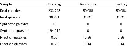
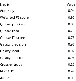
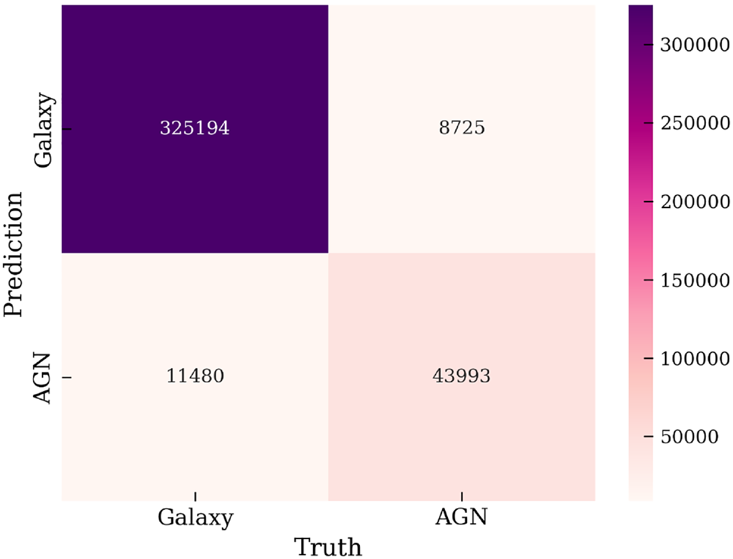
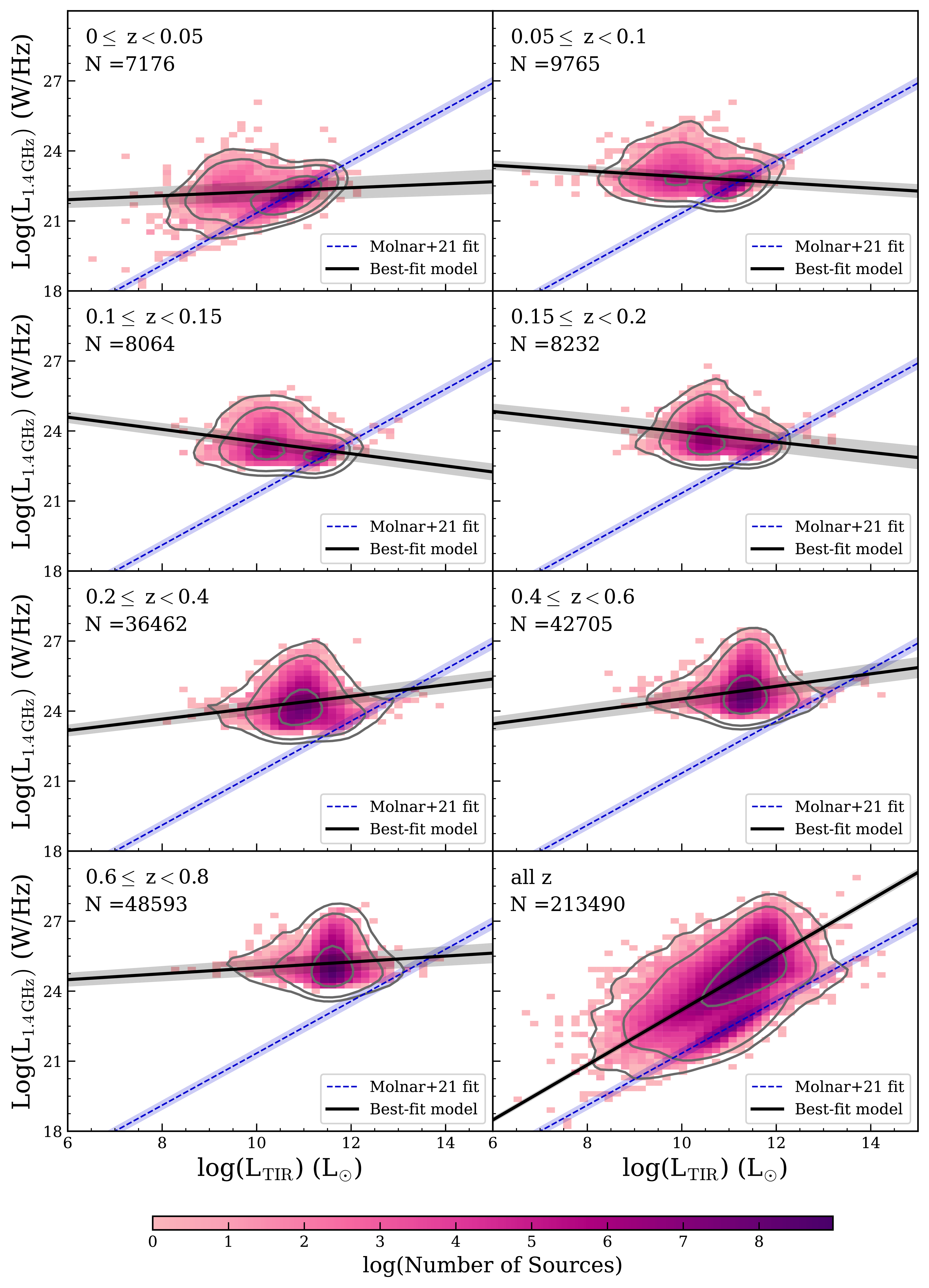
 1σ
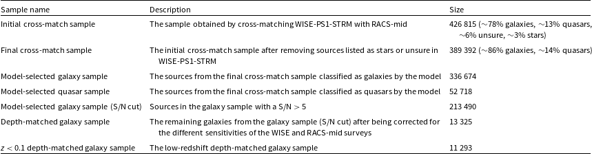
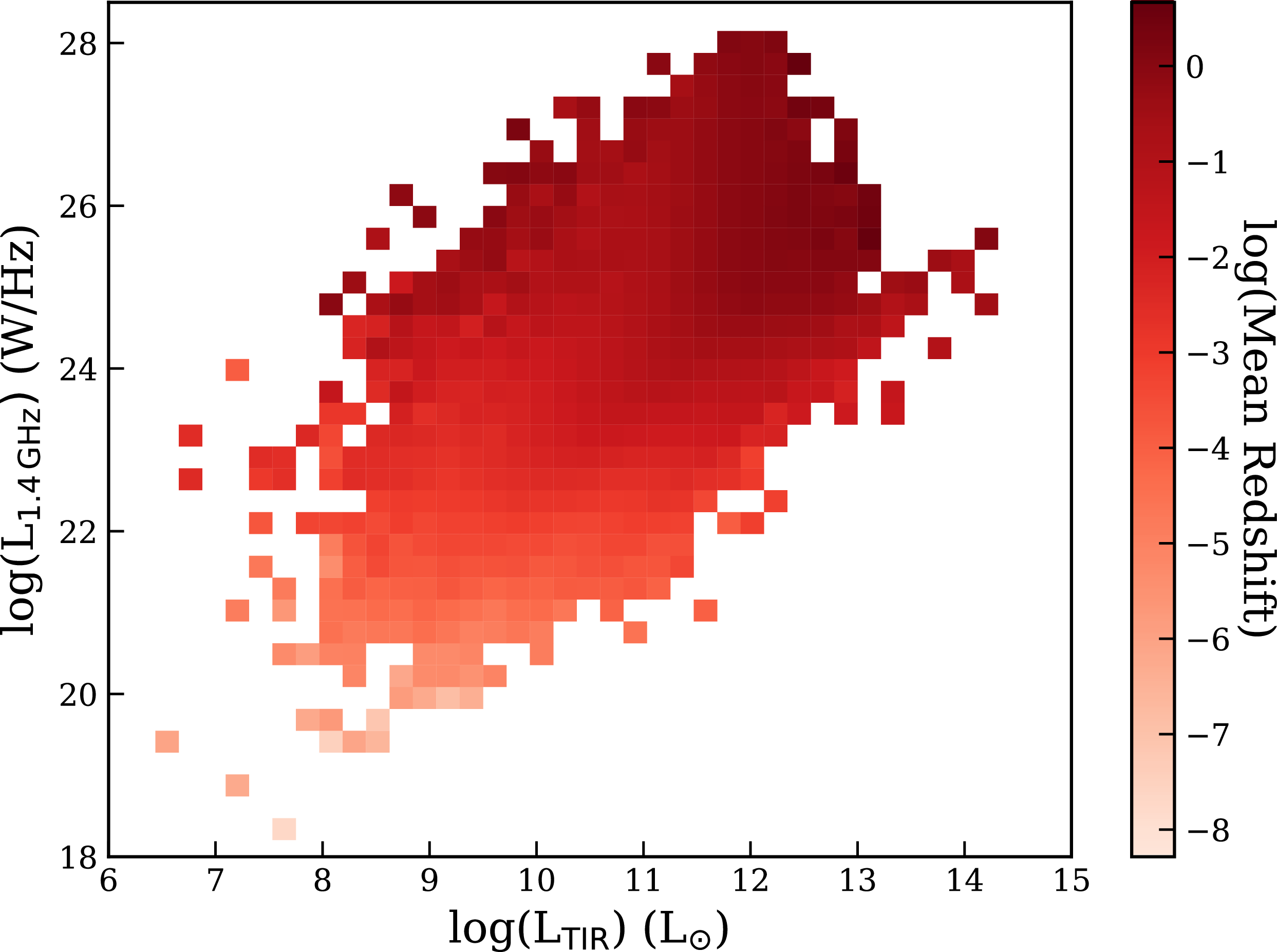
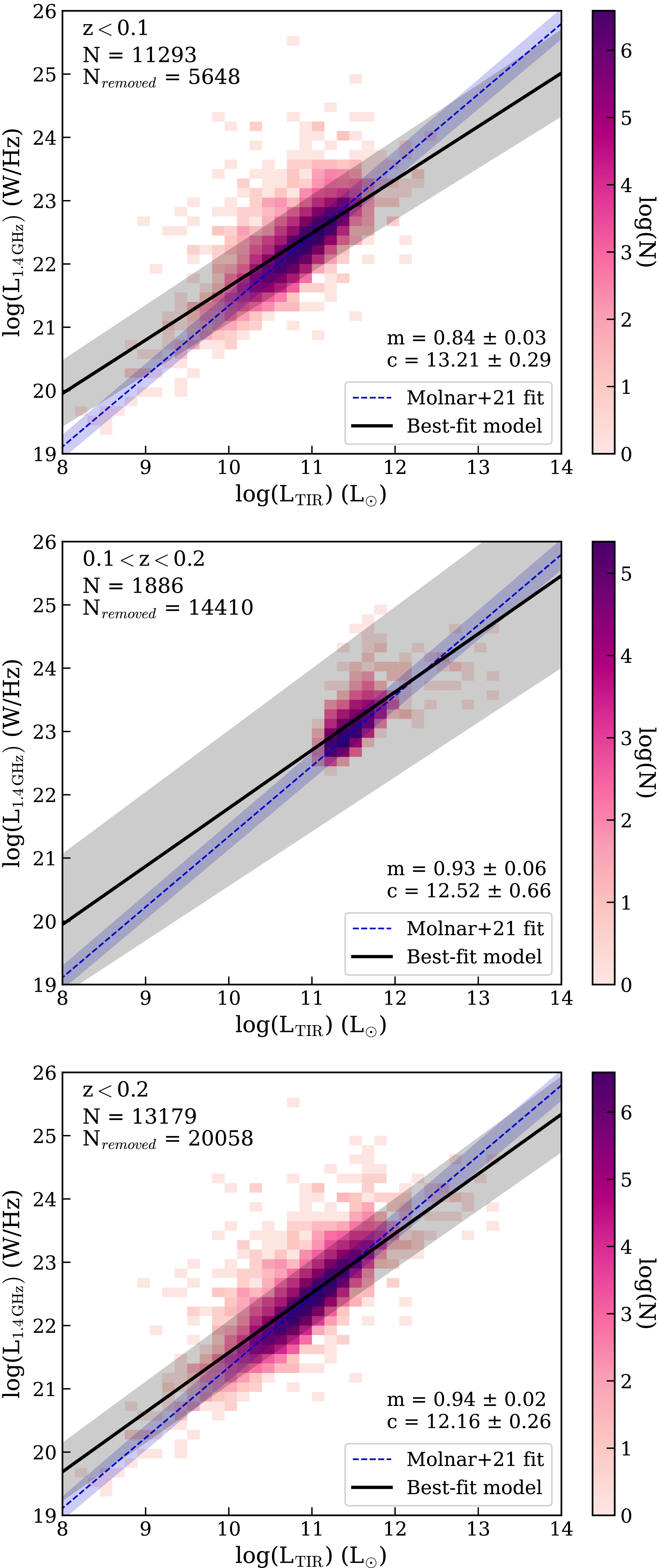
 z<0.1
 0.1
 z<0.2
 Nremoved
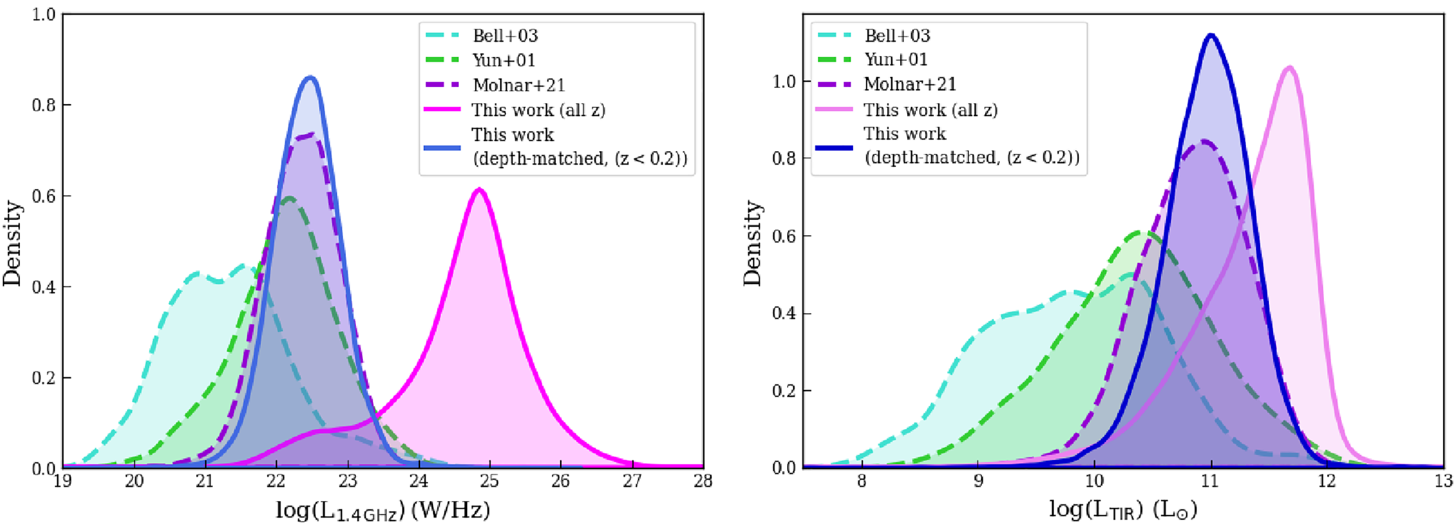
 z<0.2
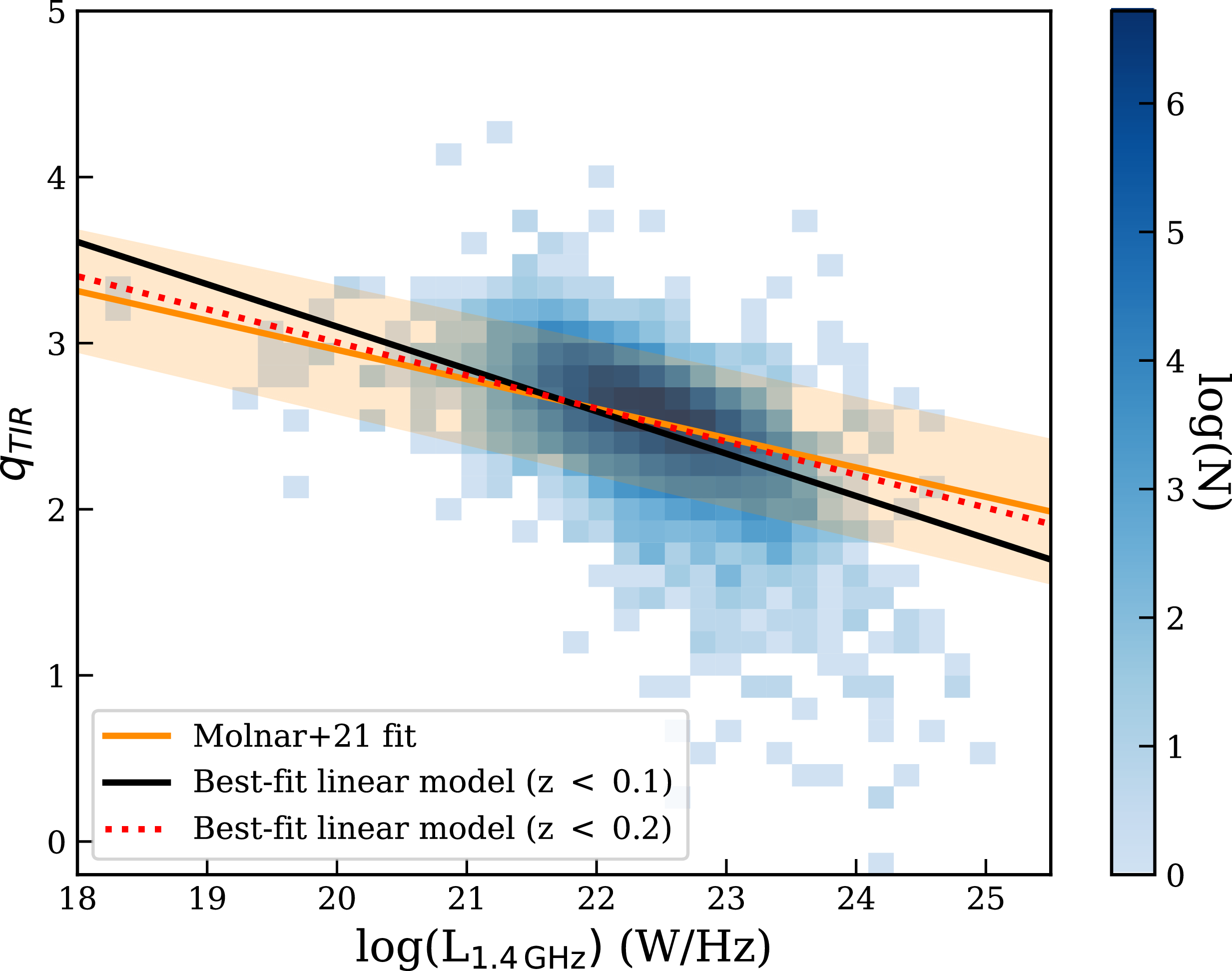
 qTIR
 log(L1.4GHz)
 z<0.1
 z<0.1
 z<0.2
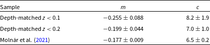
 qTIR
 log(L1.4GHz)

 σSFR
 z<0.1
 σtotal
 Vmax
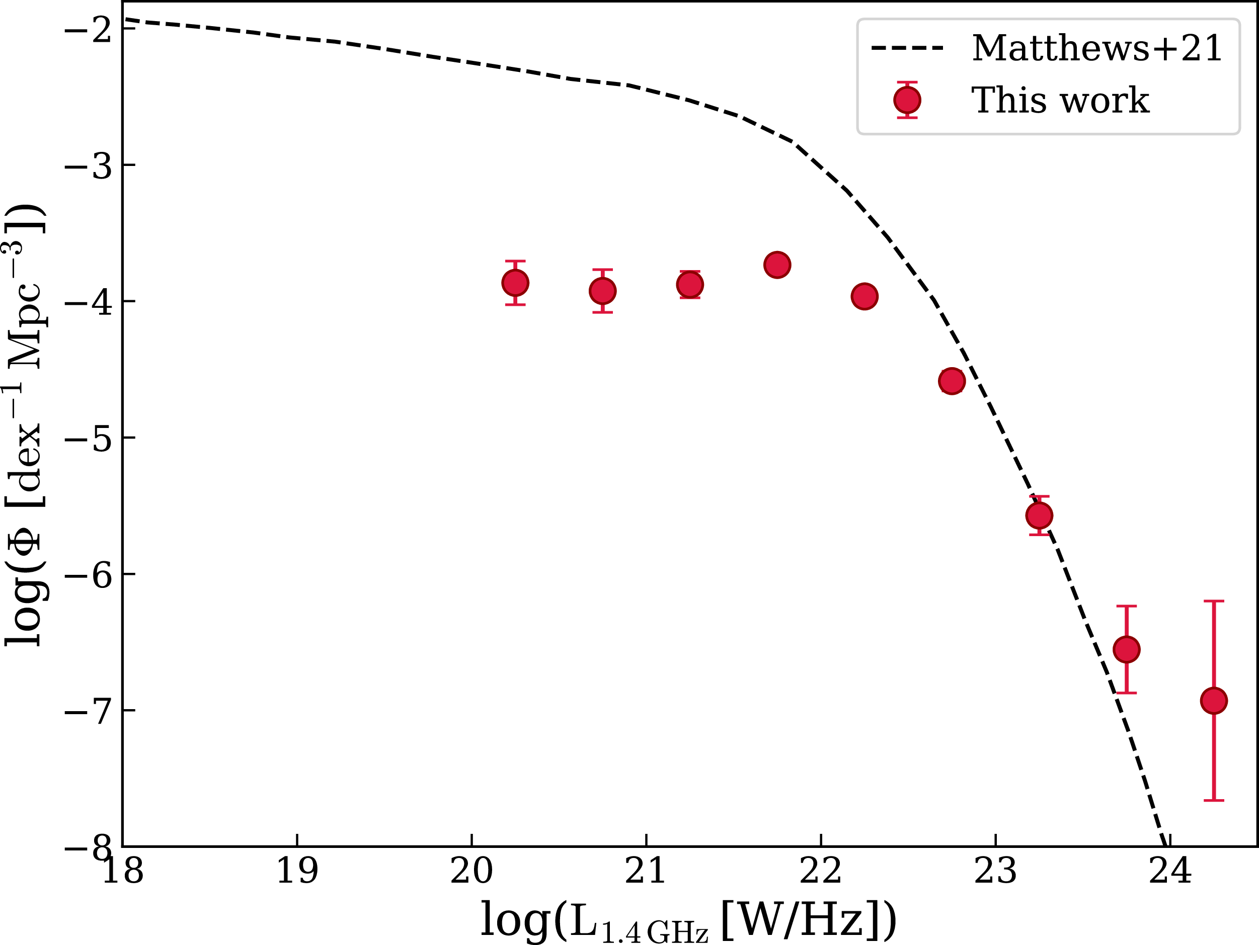
 Φ
 z<0.1
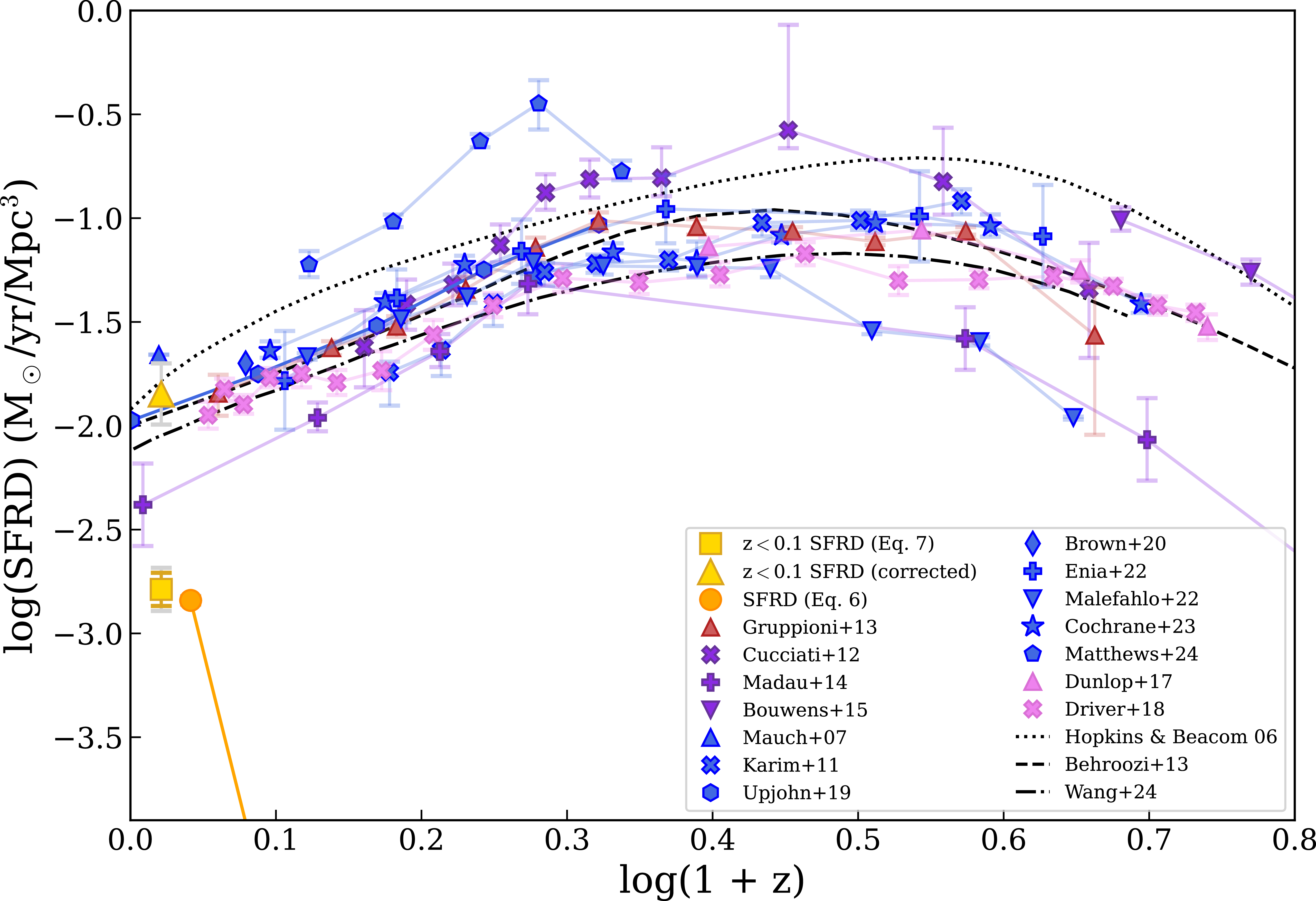
 log(1+z)
 z<0.1
 z<0.1
 z∼0.1
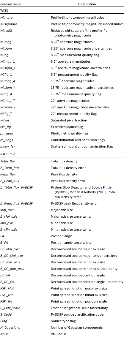
 ?
 w?mpro
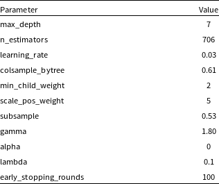
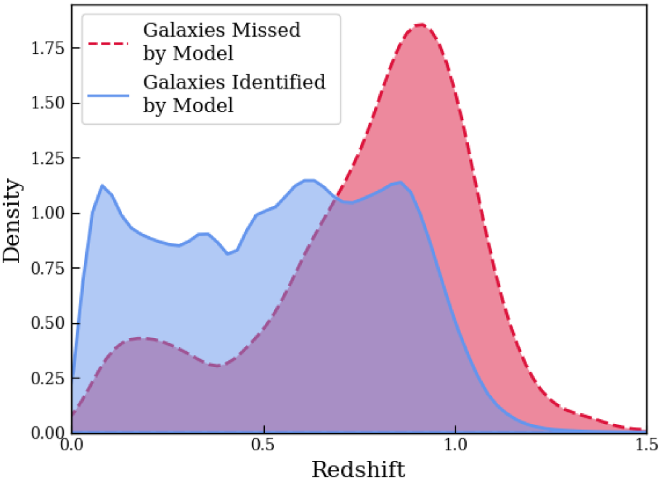
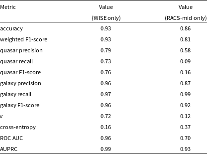
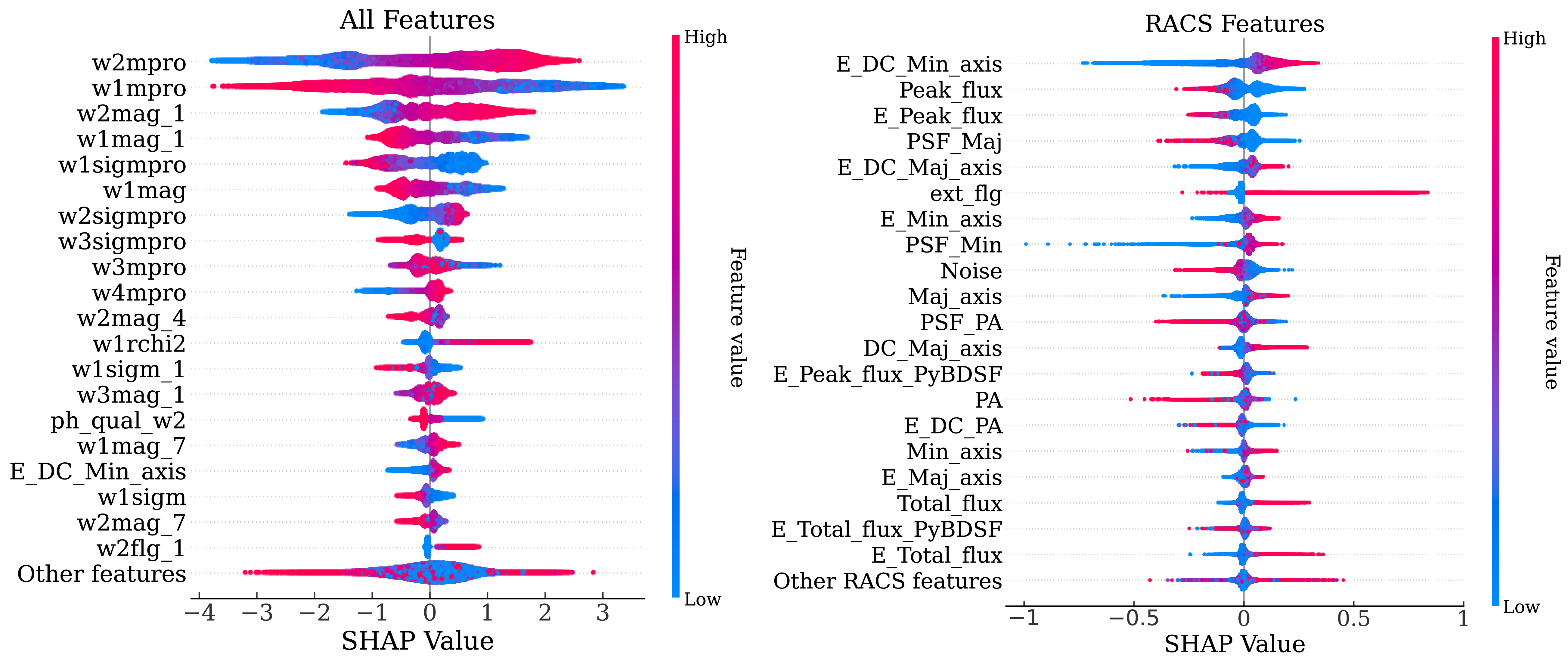
 >1
 <1
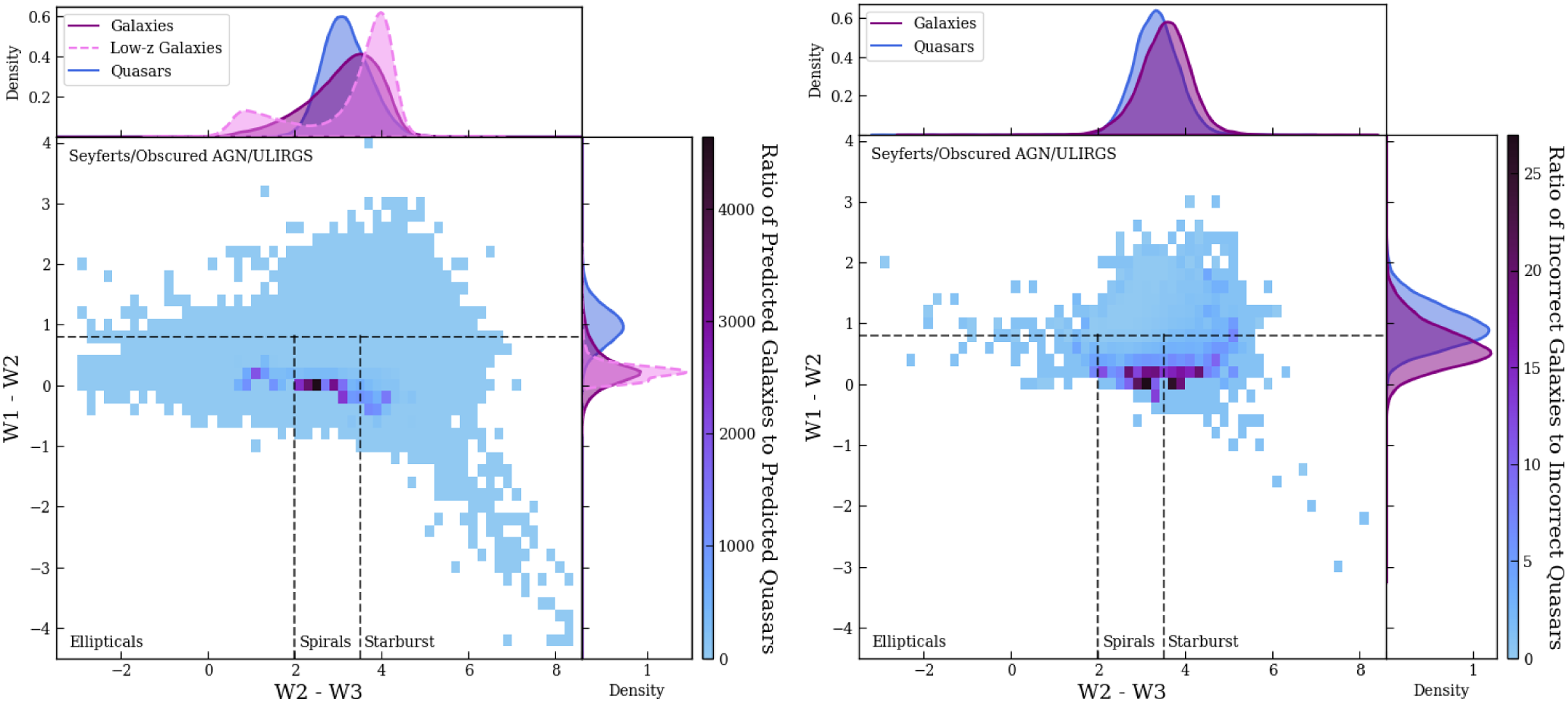
 z<0.1

 Open access

