



1. Introduction
The melting of ice into salty water is a fundamental process that occurs in various natural environments, controlling the fate of polar ice shelves, sea ice and glacial meltwater plumes (Hewitt Reference Hewitt2020; Du et al. Reference Du, Calzavarini and Sun2024; Rosevear et al. Reference Rosevear, Gayen, Vreugdenhil and Galton-Fenzi2025). Understanding its process is critical for predicting sea level rise and climate feedback mechanisms, as melting affects both local stratification and the transport of freshwater into the ocean (Jenkins Reference Jenkins1999). Recent studies have emphasised the sensitivity of melting rates to the thermodynamics at the interface (Keitzl et al. Reference Keitzl, Mellado and Notz2016), examined fluid instabilities caused by basal diffusion (Cohen et al. Reference Cohen, Berhanu, Derr and Courrech du Pont2020; Berhanu et al. Reference Berhanu, Philippi, Courrech du Pont and Derr2021), explored the role of turbulent mixing in influencing the properties of near-ice water (Couston Reference Couston2024) and investigated the asymmetries between melting and freezing within convective systems (Yang et al. Reference Yang, Xu, Verzicco and Lohse2025).
The recent numerical studies by Xue et al. (Reference Xue, Zhang and Ni2024) and Guo & Yang (Reference Guo and Yang2025), employing phase-field methods, suggest that, in the absence of external flow, the interface dynamics is controlled by the density ratio
 $R_\rho$
, a non-dimensional number defined later in (2.6), which is proportional to ambient ocean salinity and reflects the balance between the temperature and salinity effects on density. Over relatively fresh ambient water (small
 $R_\rho$
), mixing is dominated by thermal convection, and ice melts relatively rapidly in time, following a sub-diffusive scaling
 $\propto t^{-r}$
with the exponent
 $r \lesssim 0.2$
. Over relatively salty ambient water (large
 $R_\rho$
), the system instead develops a strongly stratified, diffusion-dominated regime, with the melt rate exhibiting a diffusive scaling
 $\propto t^{-0.5}$
, as also reported by Middleton et al. (Reference Middleton, Vreugdenhil, Holland and Taylor2021).
Here, we revisit the turbulence generated by a block of freshwater ice immersed in initially quiescent, warm, salty ocean water. In Xue et al. (Reference Xue, Zhang and Ni2024) and Guo & Yang (Reference Guo and Yang2025), the physics of the melting interface is treated in considerable detail, making nonlinear effects away from the interface difficult to isolate. Our setting explores the opposite limit: a simplified modelling of the interface, allowing nonlinear effects away from it to be more clearly assessed. Our study focuses on the early-time growth of the mixing layer (i.e. while unaffected by the bottom boundary) and its connection to the melt rate at the ice–ocean interface. We use high-resolution numerical simulations of the Boussinesq system under a linearised equation of state, inside a vertically bounded and horizontally periodic two-dimensional domain – supplemented by a slowly melting condition at the top boundary. We investigate how the Lewis number (the ratio of thermal to saline diffusivity) and the density ratio impact the dynamics.
In our configuration, a convective mixing layer develops, which grows super-diffusively
 $\propto t^{1.33}$
and self-similarly in time. The growth rate is largely universal, as it does not depend on double-diffusive effects, which are absent in the bulk, nor on the melt rate at the top boundary. Over sufficiently saline environments, we recover the formation of a meltwater boundary layer, which produces a diffusive regime of melting. The interfacial layer does not suppress the turbulence inside the convective mixing layer, nor does it significantly modify its statistics. However, it regulates the amount of meltwater poured into the bulk: we find that the ratio between the convective and diffusive contributions to the solutal fluxes decreases at a rate
 $\propto (\textit{LeR}_\rho )^{-1}$
, depending on both the Lewis number
 $\textit{Le}$
, representing the ratio of thermal to salt diffusivity, and the density ratio
 $R_\rho$
, representing the balance between the thermal and salinity effects on density. Because of its relative simplicity, our setting allows for some theoretical understanding of the meltwater transport, from the diffusive to the convective stages.
The paper is organised as follows: § 2 describes the physical and numerical set-up, § 3 presents the main results, contrasting the interface and bulk dynamics and discussing mixing length definitions. Finally in § 4, we share some concluding remarks. Additional technical details related to numerical set-ups and theoretical arguments are described in the appendices.
2. Numerical set-up
We consider the flow illustrated in figure 1, which is initially quiescent. The domain is two-dimensional, with horizontal extent
 $L_x$
and depth
 $L_z= L_x$
. The initial salinity
 $S$
is uniform and equal to the far-field value
 $S_\infty$
, while the temperature
 $T$
has a step profile characterised by a temperature jump
 $\Delta T = T_\infty - T_m(S_\infty )$
. This represents the difference between the far-field temperature
 $T_\infty$
and the melting temperature
 $T_m(S_\infty )= T_{f,0} + \lambda _1 S_\infty$
.
Initial configuration.

We later work with non-dimensional variables for temperature and salinity, defined as
 \begin{align} \begin{split} \theta &= \dfrac {T-T_\infty }{\Delta T} \quad \text{and} \quad \sigma = \dfrac {S-S_\infty }{\Delta S}\\ \text{where }\quad & \Delta T:= T_\infty -T_m(S_\infty ), \quad \Delta S :=\dfrac {\beta _T}{\beta _S} \Delta T. \end{split} \end{align}
Here,
 $\Delta S$
is the salinity variation required to compensate the density change caused by
 $\Delta T$
, according to the linearised equation of state
 \begin{align} \rho = \rho _0 \left [1- \beta _T T + \beta _S S \right ], \end{align}
which we adopt here for simplicity. Here,
 $\beta_T$
and
 $\beta_S$
denote the thermal expansion coefficient and the haline contraction coefficient, respectively. We model the fluid dynamics with the two-dimensional incompressible Navier–Stokes equations under the Boussinesq approximation.
Defining the horizontal length
 $L_x$
, the velocity
 $U_0 :=\sqrt {2 g \beta _T \Delta \textit{TL}_x }$
, where
 $g$
is the acceleration due to gravity, and the time
 $t_0= L_x/U_0$
, as characteristic scales, the equations of motion take the dimensionless form
 \begin{align} \begin{split} \partial _t \boldsymbol{u} + (\boldsymbol{u} \boldsymbol{\cdot }\boldsymbol{\nabla }) \boldsymbol{u} +\boldsymbol{\nabla }p & = \textit{Rey}^{-1} \Delta \boldsymbol{u} + \boldsymbol{e_z} \frac {\theta -\sigma }{2}, \quad \quad \boldsymbol{\nabla }\boldsymbol{\cdot }\boldsymbol{u} = 0, \\ \partial _t \theta + (\boldsymbol{u} \boldsymbol{\cdot }\boldsymbol{\nabla }) \theta &= \textit{Rey}^{-1} \, \textit{Pr}^{-1} \Delta \theta , \\ \partial _t \sigma + (\boldsymbol{u} \boldsymbol{\cdot }\boldsymbol{\nabla }) \sigma &= \textit{Rey}^{-1} \, \textit{Pr}^{-1} \, \textit{Le}^{-1} \Delta \sigma , \end{split} \end{align}
with non-dimensional parameters
 \begin{align} \textit{Rey} = \dfrac {U_0 L_x}{\nu }\text{(Reynolds)},\quad \textit{Pr}=\dfrac {\nu }{\kappa _T}\text{ (Prandtl)} \quad \text{and} \quad \textit{Le} = \dfrac {\kappa _T}{\kappa _S} \text{ (Lewis)}. \end{align}
The Prandtl and the Lewis numbers represent the ratio of viscosity to thermal diffusivity and thermal to salt diffusivity, respectively.
The boundary conditions represent a (no-slip) melting ice–ocean interface at the top coupled to a far-field quiescent state at the bottom, similar to Couston (Reference Couston2024). At the top boundary, the temperature
 $\theta$
is set equal to the local melting temperature, which depends linearly on salinity. This condition is supplemented by a balance between heat and haline fluxes, which determine the melt rate following the widely adopted Stefan condition (Gayen et al. Reference Gayen, Griffiths and Kerr2016; Vreugdenhil & Taylor Reference Vreugdenhil and Taylor2019; Middleton et al. Reference Middleton, Vreugdenhil, Holland and Taylor2021). The conditions read in dimensionless form
 \begin{align} \left \{ \begin{aligned} &z=0 \quad \text{(melting)}:\; \theta =-1 -\gamma _1 \sigma \quad \text{and} \quad \dfrac { \partial _z \sigma }{(\sigma + R_\rho )} = \textit{Le} \textit{St} \partial _z \theta \\ &z=-1 \quad \text{(far field)}: \quad \theta = 0 \quad \text{and} \quad \sigma = 0, \end{aligned} \right . \end{align}
with
 \begin{align} R_\rho = \dfrac {S_\infty }{\Delta S } \text{ (density ratio)}, \; \gamma _1=- \lambda _1 \dfrac {\beta _T}{\beta _S} \text{ (freezing coupling),} \; \textit{St} = \dfrac {C_p}{L_f} \Delta T \text{ (Stefan)}. \end{align}
The density ratio
 $R_\rho$
quantifies the balance between the stabilising effect of the far-field salinity and the destabilising temperature difference. The parameter
 $\gamma _1$
represents a freezing coefficient coupling temperature and salt at the meting interface; the Stefan number
 $\textit{St}$
characterises the relative importance of specific and latent heat, based on the initial temperature jump at the interface. These boundary conditions are approximations that hold true only when the melting rate is slow. Essentially, they substitute the mass flux resulting from the phase change with a diffusive flux, introducing a Lewis number dependence in (2.5). This approach serves as an alternative to directly solving the Stefan problem, which, strictly speaking, requires explicit treatment of a moving interface – see, e.g. Huppert (Reference Huppert1990) and Wettlaufer (Reference Wettlaufer2001). While phase-field methods can be employed to this end, they prove computationally expensive for small melting rates, which produce a large time-scale separation between the dynamics of phase change and that of the fluid (Favier et al. Reference Favier, Purseed and Duchemin2019; Gastine & Favier Reference Gastine and Favier2025).
Our numerical set-up employs direct numerical simulations using the finite-volume code Oceananigans (Ramadhan et al. Reference Ramadhan, Wagner, Hill, Campin, Churavy, Besard, Souza, Edelman, Ferrari and Marshall2020). The computational domain is discretised on a grid of
 $8192^2$
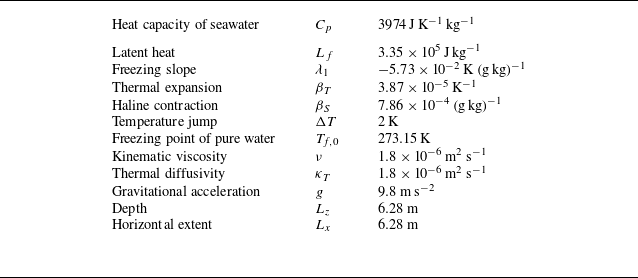
collocation points, uniform in the horizontal direction and refined vertically near the top interface. For this resolution, the spectrum of the scalar fields exhibits a clear decay at high wavenumbers (not shown), indicating that the smallest dynamically active scales are adequately resolved by the numerical grid. Since Oceananigans operates with dimensional variables, all governing parameters are prescribed in physical units, for consistency with realistic seawater properties (Allende et al. Reference Allende, Treguier, Lique, de Boyer Montégut, Massonnet, Fichefet and Barthélemy2024; Couston Reference Couston2024). They are summarised in table 1, and prescribe the free-fall velocity and time units as
 $U_0 \approx 0.098 \rm \, m\,s^{-1}$
and
 $t_0 \approx 64\rm\, s \,$
, respectively.
Physical parameters.

Table 1. Long description
A table listing physical parameters related to seawater properties. The table has 12 rows and 2 columns. The first column lists the parameters, and the second column lists their corresponding values. Row 1: Heat capacity of seawater, 3974 J K^-1 kg^-1. Row 2: Latent heat, 3.35 x 10^5 J kg^-1. Row 3: Freezing slope, -5.73 x 10^-2 K (g kg)^-1. Row 4: Thermal expansion, 3.87 x 10^-5 K^-1. Row 5: Haline contraction, 7.86 x 10^-4 (g kg)^-1. Row 6: Temperature jump, 2 K. Row 7: Freezing point of pure water, 273.15 K. Row 8: Kinematic viscosity, 1.8 x 10^-6 m^2 s^-1. Row 9: Thermal diffusivity, 1.8 x 10^-6 m^2 s^-1. Row 10: Gravitational acceleration, 9.8 m s^-2. Row 11: Depth, 6.28 m. Row 12: Horizontal extent, 6.28 m.
In all the simulations, we set
 $\Delta T = 2\,\mathrm{K}$
. To explicity satisfy the boundary conditions (2.5), we regularise the initial temperature jump by introducing a smooth temperature profile controlled by the (small) parameter
 $\delta \ll L_x$
– see figure 1. The parameter
 $\delta$
sets the initial gradient
 $\propto \Delta T /\delta$
, and offsets it down from the upper boundary, at a depth
 $\propto \delta$
. This smoothing ensures that the temperature gradient vanishes at the top boundary, hence fulfilling the boundary condition (2.5) imposed by the uniform salinity profile. To trigger the instability, the initial temperature profile of figure 1 is perturbed by a random noise of small amplitude – see Appendix A for additional details. Our series of simulations vary the Lewis number from
 $1$
to
 $100$
, keeping the thermal diffusivity constant. The density ratio
 $R_\rho$
varies from
 $1$
to
 $406$
, tracking modifications in
 $S_\infty$
. The parameters in table 1 additionally prescribe the non-dimensional values:
 $\textit{Pr}=1$
,
 $\textit{St}=2.4 \times 10^{-2}$
and
 $\gamma _1=2.8 \times 10^{-3}$
, representative of polar ice–ocean conditions, although slightly idealised for numerical efficiency – in particular
 $\textit{Pr} =O(10)$
in seawater. Additional simulations at
 $\textit{Pr}=7$
(not shown) display similar flow behaviours.
From an oceanographic perspective, please note that
 $R_\rho =O(10)$
corresponds to weakly saline conditions (
 $S_\infty \sim 1\,\rm g/kg$
), which are representative of near-surface environments influenced by strong freshwater inputs. By contrast, values
 $R_\rho \gtrsim 300$
corresponds to typical open-ocean salinities
 $S_\infty \gtrsim 30\,\rm g/kg$
encountered in polar oceans (Peralta-Ferriz & Woodgate Reference Peralta-Ferriz and Woodgate2015). For these values, the linearised equation of state (2.2) predicts that the density decreases monotonically with the temperature and this is consistent with the observations – see, e.g. Millero (Reference Millero2010) and Talley (Reference Talley2011)). While the linearised equation of state is less accurate at lower salinities, it still provides a well-defined hydrodynamical framework, allowing for a systematic investigation of the nonlinear melting dynamics and its sensitivity to key control parameters. In the present study, we therefore deliberately adopt a linear equation of state to retain a tractable framework and isolate the dominant physical mechanisms. The effects of a nonlinear equation of state, including the freshwater density anomaly, have been investigated in recent studies (e.g. Yang et al. Reference Yang, Howland, Liu, Verzicco and Lohse2023; Xu et al. Reference Xu, Yang, Verzicco and Lohse2025) and are beyond the scope of the present work.
3. Results
In all simulations, the fluid evolves through three main phases. This is illustrated in figure 2, showing representative temperature and salinity snapshots. The system initially develops a Rayleigh–Taylor (RT)-like instability, which arises from the initially unstable buoyancy jump away from the interface (Drazin & Reid Reference Drazin and Reid2004; Boffetta & Mazzino Reference Boffetta and Mazzino2017). This is followed by the interaction of the flow with the upper boundary and the onset of melting. Eventually, a mixing layer develops near the upper boundary and gradually deepens, with cold and fresh plumes extending downward into the domain. Note that, contrary to previous studies with similar configurations (Guo & Yang Reference Guo and Yang2025), we here focus on the transient dynamics before the turbulent layer reaches the bottom of the numerical domain and will not comment on the subsequent stationary (or quasi-stationary) states. Varying
 $\textit{Le}$
and
 $R_\rho$
, the main difference is seen not in the bulk but at the melting interface. Increasing
 $R_\rho$
, the top interfacial layer of fresh water gets thicker, as seen from the horizontally averaged salinity profiles in figure 3. No obvious difference is seen for the temperature, neither in the bulk nor at the interface. These observations suggest the following phenomenology: salty environments favour strong stratification between the relatively fresh meltwater layer and the ambient ocean, leading to a stable diffusive layer, while low density ratios favour mixing close to the upper interface.
Typical evolution of the temperature (a) and salinity fields (b) for a simulation with
 $\textit{Le} = 100$
and
 $R_\rho = 406$
.

(a) Temporal evolution of the horizontally averaged salinity profile for
 $\textit{Le} = 100$
and
 $R_\rho = 406$
. (b) Same but for
 $\textit{Le} = 100$
and
 $R_\rho = 1$
.

3.1. Fluxes and temperature at the top interface
To quantify the melt rate, we introduce the Nusselt number
 \begin{align} \textit{Nu} = - \left \langle \partial _{ z} \theta \right \rangle _{z=0}, \end{align}
with
 $\langle \boldsymbol{\cdot }\rangle$
denoting horizontal averaging. Analogous to Rayleigh–Bénard (RB) convection, the Nusselt number measures the thermal flux at the top boundary in units of the average temperature gradient
 $\Delta T/L_x$
– recall that
 $L_x =1$
in our length units. It is directly proportional to the melt rate,
 $\textit{Nu} \propto \textit{Le} \, \textit{St} \partial _z \theta |_{z=0}$
. With the conventional minus sign in (3.1), the regime
 $\textit{Nu} \gt 0$
reflects melting (this is the case under study) while
 $\textit{Nu}\lt 0$
would indicate freezing. Unlike RB convection,
 $\textit{Nu}$
decays over time. Its algebraic rate of decay exhibits two distinct asymptotic regimes, highlighting a strong dependence on the density ratio
 $R_\rho$
and only a weak dependence on
 $\textit{Le}$
– see figure 4. In fresh environments, i.e. for small values of
 $R_\rho \lesssim 10$
, the Nusselt number decays only mildly as
 $\textit{Nu} \sim C_f t^{-0.2}$
, where both the exponent and the prefactor are insensitive to the Lewis number. In salty environments, i.e., for large values of
 $R_\rho \gtrsim 10$
, we observe a diffusive scaling
 $\textit{Nu} \sim C_s t^{-0.5}$
, with the prefactor following the apparent scaling law
 $C_s \sim \textit{Le}^{a} R_\rho ^{b}$
. Our simulations indicate
 $ a\simeq 0.1$
and
 $b\simeq -0.3$
, meaning that the Lewis number and density ratio have opposite effects, respectively enhancing and slowing melting in this apparent diffusive regime.
Time evolution of the Nusselt number
 $\textit{Nu}$
, varying
 $R_\rho$
for fixed
 $\textit{Le}$
(a,b) and
 $\textit{Le}$
for fixed
 $R_\rho$
(c,d). In all four panels, the insets display the prefactors
 $C_s, C_f$
(see text) averaging over times
 $ t \gtrsim 10$
.

The salinity at the boundary modifies the freezing temperature at the interface. Figure 5 shows the evolution with time of the excess temperature (i.e. above the freezing temperature based on the far-field salinity)
 \begin{align} \theta _0 := 1+\left \langle \theta \right \rangle _{x,z=0} =-\gamma _1 \sigma _0, \end{align}
where
 $\sigma _0=\langle \sigma \rangle _{x,z=0}$
. The second equality indicates that
 $\theta _0$
is proportional to the horizontally averaged fluctuation in salinity – see (2.5). Positive fluctuations
 $\theta _0 \geqslant 0$
are associated with fresh water at the interface,
 $\sigma _0 \leqslant 0$
. Unlike the Nusselt number, no clear dichotomy emerges. In all the simulations, the top temperature quickly reaches a quasi-stationary value, yielding the scaling behaviour
 $\theta _0 \propto \textit{Le}^{0.5} R_\rho$
. Theoretically, this scaling reflects a diffusive dynamics near the melting boundary – see Appendix B. It is consistent with the intuitive idea that saltier ambient water favours a comparatively fresher interfacial boundary layer near the top interface.
Time evolution of the excess temperature
 $\theta _0$
, varying
 $R_\rho$
at fixed
 $\textit{Le}$
(a,b) and
 $\textit{Le}$
at fixed
 $ R_\rho$
(c,d). In all four panels, the insets display the dependence on either
 $R_\rho$
or
 $\textit{Le}$
averaging over times
 $ t \gtrsim 10$
.

Figure 5. Long description
Panel A: A line graph shows the time evolution of the excess temperature for a Lewis number of 1. The x-axis represents time on a logarithmic scale ranging from 10^0 to 10^2. The y-axis represents the excess temperature on a logarithmic scale ranging from 10^-5 to 10^1. Multiple lines of different colors indicate different data series. The inset graph shows the dependence of the initial excess temperature on the density ratio, with a dotted line indicating a proportional relationship. Panel B: A line graph shows the time evolution of the excess temperature for a Lewis number of 100. The x-axis represents time on a logarithmic scale ranging from 10^0 to 10^2. The y-axis represents the excess temperature on a logarithmic scale ranging from 10^-5 to 10^1. Multiple lines of different colors indicate different data series. The inset graph shows the dependence of the initial excess temperature on the density ratio, with a dotted line indicating a proportional relationship. Panel C: A line graph shows the time evolution of the excess temperature for a density ratio of 1. The x-axis represents time on a logarithmic scale ranging from 10^0 to 10^2. The y-axis represents the excess temperature on a logarithmic scale ranging from 10^-5 to 10^1. Multiple lines of different colors indicate different data series. The inset graph shows the dependence of the excess temperature on the Lewis number, with a dotted line indicating a proportional relationship. Panel D: A line graph shows the time evolution of the excess temperature for a density ratio of 406. The x-axis represents time on a logarithmic scale ranging from 10^0 to 10^2. The y-axis represents the excess temperature on a logarithmic scale ranging from 10^-5 to 10^1. Multiple lines of different colors indicate different data series. The inset graph shows the dependence of the excess temperature on the Lewis number, with a dotted line indicating a proportional relationship.
3.2. Meltwater transport: from diffusion to convection
Our set-up employs a regularisation that offsets the initial temperature jump between the ice and the underlying bulk fluid by a depth
 $\delta \ll 1$
. This triggers a classical RT turbulent mixing layer. Without an upper boundary, the layer would grow quadratically
 $L(t)\sim t^2$
under a critical balance between buoyancy and nonlinear terms – this is the self-similar Bolgiano–Obukhov scenario (Chertkov Reference Chertkov2003; Boffetta & Mazzino Reference Boffetta and Mazzino2017). The interaction with the top interface, however, disrupts this classical regime by creating a (meltwater) boundary layer that couples the melting interface to the turbulent mixing layer. To characterise the exchange between the boundary layer and the turbulent layer, we examine the vertical fluxes of temperature and salinity. After horizontal averaging, each flux can be decomposed into convective and diffusive contributions as
 \begin{align} \phi _\chi = \phi _\chi ^c + \phi _\chi ^d,\quad \phi _\chi ^c = \left \langle \chi u_z \right \rangle ,\quad \phi _\chi ^d = -\lambda _\chi ^{-1} \textit{Pr}^{-1}\textit{Rey}^{-1} \left \langle \partial _z \chi \right \rangle , \quad \chi \equiv \theta ,\sigma, \end{align}
with
 $\lambda _\theta = 1$
and
 $\lambda _\sigma =\textit{Le}$
. Figure 6 illustrates the generic behaviour using the most saline environment
 $R_\rho =406$
at
 $\textit{Le}=100$
, highlighting two propagation rates. At any time during the growth, the convective fluxes
 $\phi _\theta ^c,\phi _\sigma ^c$
fluctuate in
 $z$
about a nearly constant value before dropping sharply. These drops become synchronised from
 $t\gtrsim 2$
, defining the extent of the convective mixing layer. The layer propagates superdiffusively and reaches the bottom interface at
 $t\simeq 27$
as
 \begin{align} L(t) \simeq C \, t^{\beta },\quad C \approx 0.015,\quad \beta \simeq 1.33 . \end{align}
The diffusive contributions
 $\phi _\theta ^d,\phi _\sigma ^d$
evolve on slower time scales, following the (diffusive) scalings;
 \begin{align} \delta _\chi (t) = \lambda _\chi ^{-1/2}\textit{Rey}^{-1/2}\textit{Pr}^{-1/2} t^{1/2},\quad \chi \equiv \theta ,\sigma; \end{align}
see Appendix A. In figure 6, this differential propagation is signalled by the collapse of the convective and diffusive fluxes shown in the panels (c), (d), (e) and (f). These collapses are obtained by rescaling lengths with the superdiffusive scaling (3.4) and the diffusive scaling (3.5), respectively. At each time, the cross-overs between diffusive and convective contributions define the effective boundary layer thicknesses
 $\propto \delta _\theta ,\delta _\sigma$
for the solutal and thermal field, respectively. Within this layer, the transport of meltwater is diffusive and hence sensitive to double-diffusive effects. Below this layer, solutal and thermal transport is convective, but in a non-trivial way. While this convection originates from the nonlinear stages of the initial RT instability, it does not propagate following the critical-balance scaling
 $\propto t^2$
. Instead, the superdiffusive rate (3.4) reflects the presence of a boundary at
 $z=0$
.
(a,b) Vertical fluxes at successive times for the case
 $\textit{Le} = 100$
and
 $R_\rho = 406$
, decomposed into their diffusive (solid lines) or convective (dashed lines) contributions. (c,d) Diffusive contributions rescaled using the diffusive scaling
 $\delta _\chi (t) \propto t^{1/2}$
. (e,f) Convective contributions rescaled using the superdiffusive scaling
 $L(t) \propto t^{4/3}$
. Panels (a, c, e) are for the thermal fluxes. Panels (b, d, f) are for the solutal fluxes.

3.3. Constant-in-space heat flux scenario for the superdiffusive growth
 $\propto t^{4/3}$

The collapse in figure 6 with the superdiffusive rates (3.4) suggests a constant-flux propagation scenario through the domain. This can arise if the convective thermal and solutal fluxes evolve self-similarly as
 \begin{align} \phi _\chi ^c (z,t) \sim L^{-\alpha }\varPhi _{\chi }\left ( \dfrac {|z|}{L(t)}\right ) + \text{fluctuations},\quad \chi \equiv \theta ,\sigma , \end{align}
involving similarity flux profiles
 $\varPhi _\theta ,\varPhi _\sigma$
. The exponent
 $\alpha$
prescribes the decay rate
 $\propto (|z|/L)^{-\alpha }$
of the convective flux across the mixing layer. For example, setting
 $\alpha =0$
gives a scenario where the convective fluxes are approximately uniform across the mixing layer. Regardless of the exponent, the horizontally averaged fields must also be self-similar within the mixing layer
 \begin{align} \left \langle \theta \right \rangle (z,t) \sim L^{-x} \varTheta \left ( \dfrac {|z|}{L(t)}\right ) + \text{fluctuations},\quad \left \langle \sigma \right \rangle (z,t) \sim L^{-x} \varSigma \left ( \dfrac {|z|}{L(t)}\right ) + \text{fluctuations},\quad \end{align}
for some exponent
 $x \geqslant 0$
. This form implies the algebraic behaviour
 $\propto (|z|/L)^{-x}$
far away from the front but within the mixing layer, i.e.
 $\delta _\theta ,\delta _\sigma \ll |z| \ll L$
– see, e.g. Barenblatt (Reference Barenblatt1996) and Campolina et al. (Reference Campolina, Simonnet and Thalabard2025)). In turn, this prescribes the behaviours for the similarity profiles
 \begin{align} \varPhi _{\chi }(\eta ) \sim |\eta |^{-\alpha },\quad \varSigma (\eta ),\; \varTheta (\eta ) \sim |\eta |^{-x}\quad |\eta |\ll 1. \end{align}
Assuming an algebraic growth
 $L\propto t^\beta$
, the dimensional balance between the transport terms
 $\partial _z \phi ^c_\theta$
and
 $\partial _t \langle \theta \rangle$
prescribes that the three exponents
 $\beta ,x,\alpha$
satisfy
 \begin{align} \beta (1+\alpha -x)=1. \end{align}
Provided that
 $x\lt 1$
, then the temperature field evolves as
 \begin{align} \dfrac {d}{{\rm d}t}\int _{-\infty }^0 {\rm d}z \; \theta (z,t) = \left \{ \begin{aligned} & (\textit{PrRe})^{-1} \textit{Nu}(t) \\ & \beta (1- x) t^{\beta -\beta x -1} \int _{0}^1\varTheta (\eta ) {\rm d}\eta \propto t^{-\alpha \beta }, \end{aligned} \right . \end{align}
where the first and second lines in the rhs are obtained from the boundary flux and from the self-similar scaling, respectively.
Combined with the growth exponent
 $\beta =1.33$
from (3.4), the compatibility (3.9) prescribes in particular
 $x-\alpha \simeq 0.25$
leaving only one exponent to be determined, say
 $\alpha$
. In turn, (3.10) relates the exponent
 $\alpha$
to the decay of Nusselt. The Nusselt decay
 $\textit{Nu} \propto t^{-0.2}$
reported in figure 4 suggest
 $\alpha \beta \simeq 0.2$
, implying
 $\alpha \simeq 0.15$
and
 $x \simeq 0.4$
. This scenario prescribes that the heat flux decreases with depth across the mixing layer
 $\phi _\chi \propto |z|^{-0.15}$
. On the other hand, figure 4 could possibly reflect constant behaviour
 $\textit{Nu} \propto t^{0}$
only polluted by finite-size effects. This constant-flux scenario implies
 $\alpha =0$
and
 $x\simeq 0.25$
. Both scenarios can be examined directly. To compute the universal profiles
 $\varTheta$
,
 $\varPhi _\theta$
, etc., we suppress the fluctuations in (3.6) by first rescaling
 $ z \to z/L(t)$
, multiplying by the suitable power of
 $L$
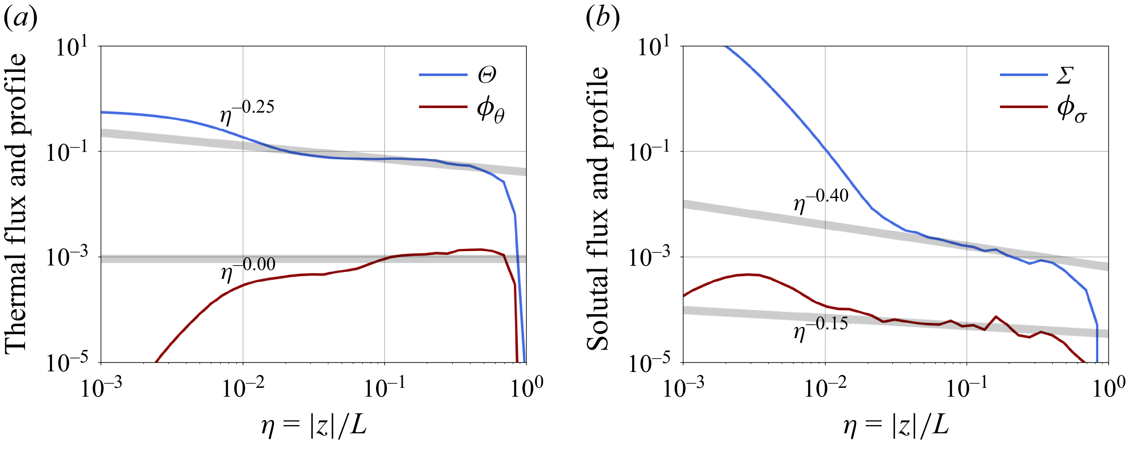
and then temporally averaging. The results are shown in figure 7. Inspection of the thermal flux supports the exponent
 $\alpha =0$
, corresponding to an approximately constant flux across the domain and implying the scaling
 $\eta ^{-0.25}$
for thermal layer away from the front. The solutal layer is rather characterised by the exponents
 $\alpha \simeq 0.15$
and
 $x\simeq 0.4$
. The difference between thermal and solutal similarity may reflect the asymmetric roles of temperature and salinity, which respectively provide destabilising and stabilising contributions to the initial density profile.
Similarity profiles obtained from the scalar fields and fluxes for
 $\textit{Le} = 100$
and
 $R_\rho = 406$
. (a) Temperature, with the exponents
 $\alpha =0,x=0.25$
. (b) Salinity with the exponents
 $\alpha =0.15,x=0.4$
.

3.4. Universality of the convective regime
The convective regime is largely insensitive to variations of the density ratio and the Lewis number. To provide a systematic estimate of the convective mixing layer, we compute
 $L(t)$
by thresholding the heat flux at a small cutoff value
 $\epsilon =10^{-12}$
, explicitly defining
 \begin{align} L(t) = \sup \left \lbrace |z|, \phi _\theta (t) \geqslant 10^{-12} \right \rbrace \!. \end{align}
Figure 8 gathers the data, revealing the universality of the superdiffusive rate (3.4) across the range of
 $\textit{Le}$
and
 $R_\rho$
investigated. This universality is compatible with the similarity scenario sketched in § 3.3: the mixing-layer growth is driven by a constant-flux similarity solution, associated with the inviscid dynamics within the bulk. The latter is obtained by formally setting
 $\textit{Rey} \to \infty$
in (2.3). This scenario explains why the constant
 $C_f$
measured in figure 4 is independent of both
 $\textit{Le}$
and
 $R_\rho$
.
(a) Time evolution of the thermal (o) and solutal (x) mixing lengths at
 $\textit{Le}=1$
for various density ratios. The vertical dashed line marks the time at which the fronts reach the bottom boundary. (b) Same but for
 $\textit{Le}=100$
.

Double-diffusive effects are present only close to the upper interface. They regulate the exchanges between the boundary meltwater layer and the turbulent mixing layer. We quantify these exchanges through the efficiency ratios
 \begin{align} \varGamma _\chi (t) = \dfrac { |\varPhi ^c_\chi (\eta =0.5)|}{|\phi ^d_\chi (z=0)|},\quad \chi \equiv \theta ,\sigma , \end{align}
estimating the relative strength of the convective flux – estimated half-way towards the front – compared with the diffusive flux at the interface. Figure 9 shows the result at a time
 $t = 10$
, when the turbulent layer is developed but occupies only
 $1/5$
of the box – still far from the bottom boundary. For the thermal fluxes, the efficiency ratio
 $\simeq 1.8$
is largely independent of the density ratio and Lewis number. A transition at
 $R_\rho \lesssim 10$
between relatively saline and relatively fresh environments is apparent for the solutal efficiency. For a fixed Lewis, the solutal efficiency varies mildy in the fresh case,
 $R_\rho \lesssim 10$
, and decreases algebraically
 $\propto R_\rho ^{-1}$
in the salty case,
 $R_\rho \gtrsim 10$
. This transition is compatible with that observed in figure 4 for the time evolution of the Nusselt number, marking the onset of the regime of diffusive decay
 $\textit{Nu} \propto t^{-0.5}$
and the formation of the (fresh) diffusive boundary layer near the top interface. This layer does not impact the statistics of turbulent mixing within the bulk, but regulates the amount of salt deficit injected into it. The efficiency decreases with Lewis; asymptotic estimates relying on the diffusive nature of the boundary layer dynamics predict
 $\propto \textit{Le}^{-1}R_\rho ^{-1}$
. Such estimates are obtained from the diffusive phenomenology described in Appendix B – in particular the gradient estimate (B3)
 $\partial _z \sigma \propto \sigma _0 \textit{Le}^{1/2}/\sqrt {t}$
and the scaling estimate (B5)
 $\sigma _0 \propto R_\rho \textit{Le}^{1/2}$
. This scaling law is shown in figure 9 and is compatible with our observations. It implies that only a small fraction
 $\propto \textit{Le}^{-1}R_\rho ^{-1}$
of the input solutal flux permeates through the interfacial layer to reach the convective layer.
Thermal flux ratio
 $\varGamma _\theta$
(circles) and solutal flux ratio
 $\varGamma _\sigma$
(crosses) for different density ratios. (a) Case
 $\textit{Le} = 1$
. (b) Case
 $\textit{Le}=100$
. The horizontal lines indicate
 $\varGamma _\theta =1.8$
(dashed) and
 $\varGamma _\sigma =\textit{Le}^{-1}$
(solid). The indicative scalings
 $\propto \textit{Le}^{-1}R_\rho ^{-1}$
share a common prefactor
 $ \simeq 30$
.

3.5. Comments on mixing lengths
At high
 $R_\rho$
, the physics involves an interplay between turbulent and diffusive flows, making the interpretation of mixing lengths strongly dependent on their practical evaluation. The mixing length
 $L(t)$
used in the previous section tracks the turbulent front, and is hence unaffected by the fresh boundary layer. It emphasises the role of thermally induced convection and is largely independent of
 $\textit{Le}$
and double-diffusive effects within the bulk.
Among various options, the temperature and salinity mixing layers could be defined from different threshold values on the scalar fields themselves, as illustrated in figure 10. We observe that the temperature mixing layer exhibits the universal super-diffusive growth
 $Ct^{1.33}$
prescribed by (3.4) regardless of the selected threshold. In contrast, the solutal mixing layer exhibits a strong dependence on the chosen threshold. For small thresholds, the definition captures the turbulent front, and the growth remains as
 $Ct^{1.33}$
. Increasing the threshold, the mixing length captures the near-interfacial dynamics, driven by the fresh, stably stratified meltwater layer. In this case, the solutal mixing length grows diffusively as
 $L_\sigma \sim D_\sigma t^{1/2}$
, with a prefactor
 $D_\sigma$
that depends on the threshold value.
Temporal evolution of the mixing length evaluated at
 $\textit{Le}=100$
and
 $R_\rho =406$
using different thresholds. (a) Thermal mixing length. (b) Solutal mixing length.

These results highlight the sensitivity of mixing diagnostics to their precise definition. Here, different thresholds probe distinct physical processes, from turbulent transport in the bulk to the diffusion-dominated dynamics near the interface. This sensitivity suggests potential caveats in more complex oceanographic settings, where mixed-layer depths are commonly defined using scalar threshold-based criteria (Allende et al. Reference Allende, Fichefet, Goosse and Treguier2023; de Boyer Montégut Reference de Boyer Montégut2024).
4. Concluding remarks
We have examined the melt-driven convection beneath an ice–ocean interface. Consistent with previous studies (Xue et al. Reference Xue, Zhang and Ni2024), our setting exhibits a subdiffusive-dominated regime
 $\propto t^{-0.2}$
at small
 $R_\rho$
and a diffusion-dominated regime
 $\propto t^{-0.5}$
at large
 $R_\rho$
in the regulation of the thermal flux at the upper boundary. However, we find that the diffusive dynamics remains confined only to a thin interfacial layer, with the bulk flow evolving through a (turbulent) convective thermal layer. Regardless of the near-interface regime, the front of the turbulent layer grows super-diffusively as
 $L \propto t^{4/3}$
for all
 $R_\rho$
and
 $\textit{Le}$
. This scaling differs from the
 $t^2$
growth associated with RT convection (Chertkov Reference Chertkov2003; Boffetta & Mazzino Reference Boffetta and Mazzino2017), reflecting the presence of a rigid lid at the top boundary. The melting boundary condition controls the solutal flux in the convective mixing layer. In particular, for large density ratios, only a fraction
 $\propto R_\rho ^{-1}$
of the meltwater input flux contributes to the solutal convective flux in the bulk.
While strongly idealised, our setting showcases a non-trivial interplay between a diffusive meltwater boundary layer and a convective interior. The interfacial layer is governed by double-diffusive effects, while turbulent transport drives the bulk. The simplicity of the setting, which represents meltwater input as a nonlinear boundary condition without explicitly resolving phase transitions, allows us to decipher the governing scaling laws. In short, the physics related to the interfacial boundary layer exhibits strong dependence on
 $\textit{Le}$
and
 $R_\rho$
, while that related to convective effects is largely universal. Our simulations suggest a constant-flux scenario across the turbulent mixing layer, implying in particular that the subdiffusive evolution of Nusselt at the boundary
 $\propto t^{-0.2}$
is a finite Reynolds number effect, likely reflective of an asymptotic regime characterised by a constant Nusselt number meltwater input.
Several questions remain relating to the detailed phenomenology of the flow and its dependence upon key physical parameters (dimensionality, initial stratifications, non-stationarity). Achieving a detailed phenomenology of melting-driven turbulence, in the spirit of the work of Chertkov (Reference Chertkov2003) on RT turbulence, constitutes a natural theoretical extension of the present work. Another issue relates to the flow universality, as the sharp interfacial gradient at the top interface makes the initial configuration effectively singular, with potential implications for its statistical predictability – see, e.g. Biferale et al. (Reference Biferale, Boffetta, Mailybaev and Scagliarini2018) and Thalabard et al. (Reference Thalabard, Bec and Mailybaev2020). To control the regularisation of the initial singularity, we chose to initiate melting through a thermal RT instability slightly offset from the interface. This physical regularisation enables the boundary conditions to be explicitly enforced at early times, and triggers the convective turbulent layer. While no dependence on
 $\delta \to 0$
, was found, it remains unclear whether such turbulent generation is universal across different regularisation schemes – in particular implementations relying on implicit regularisations only through numerical discretisation.
Acknowledgements
This work was granted access to the HPC resources of TGCC under the GENCI allocation A0170115703 (project: Simulation Numérique des Interactions entre l’Océan et la Glace de Mer). The authors acknowledge the Centre de Calcul Intensif d’Aix-Marseille for providing access to its high-performance computing resources. This work was also granted access to the HPC resources of IDRIS under the GENCI allocation 2026-A0200407543.
Funding
This work is funded by the European Union. Views and opinions expressed are however those of the authors only and do not necessarily reflect those of the European Union or the European Research Council Executive Agency. Neither the European Union nor the granting authority can be held responsible for them. S.A. was supported by the Marie Skłodowska-Curie Actions (MSCA) under grant agreement 101150225. L.-A.C. was supported by an ERC grant (IceAblation, 101117317).
Declaration of interests
The authors report no conflict of interest.
Appendix A. Details on the numerical protocol
This section provides additional information regarding our numerical protocol, detailing the initial conditions and the role of
 $\delta$
as a smoothing numerical parameter.
A.1. Initial conditions
The initial salinity field is taken to be spatially uniform,
 $S_i(x,z) = S_\infty$
. This choice prescribes both the interfacial temperature at the ice–water boundary through the freezing-point relation and the far-field temperature as, respectively,
 \begin{align} T_{\textit{top}} = T_m(S_\infty ) := T_{{f,0}} + \lambda _1 S_\infty ,\quad \quad T_\infty = T_{\textit{top}} + \Delta T. \end{align}
In order to avoid an abrupt numerical adjustment at the interface, we smooth out the temperature jump over a thin vertical layer of thickness
 $\delta$
. Specifically, we define
 $z_0 = -2\delta$
,
 $h = \delta /4$
to construct the (unperturbed) background temperature profile as
 \begin{align} T_i(z) = \dfrac { T_\infty +T_{\textit{top}}\exp \left (2\frac {z-z_0}{h}\right ) }{ 1+\exp \left (2\frac {z-z_0}{h}\right ) }, \end{align}
which interpolates between
 $T_i(-\infty ) = T_\infty$
and
 $T_i(0) = (T_\infty e^{-16} + T_{top} )/(e^{-16}+1) \simeq T_{top}$
. This temperature field has a vanishing gradient at the top interface and therefore satisfies the boundary condition (2.5) with the constant field
 $S_i(x,z)=S_\infty$
. To seed instabilities, the temperature field is perturbed by small-amplitude Gaussian random noise, drawn independently and everywhere in space as
 \begin{align} T_i^{\epsilon }(x,z) = T_i(z) + \sqrt {\epsilon } \eta (x,z) \quad \eta (x,z) \sim \mathcal{N}\!\left (0,1\right ). \end{align}
In our simulations, we typically set
 $\epsilon = 10^{-10}$
and
 $\delta =0.05\,L_z$
.
A.2. Numerical implementation of the boundary conditions
At the ice–ocean interface, the dimensional version of the melting boundary conditions (2.5) involve the top salinity
 $S_{\textit{top}}=S(z=0)$
and the temperature
 $T_{\textit{top}}=T(z=0)$
, together with their derivatives as
 \begin{align} T_{\textit{top}} = T_m(S_{\textit{top}}) \text{ (melting point)} \quad \text{ and }\quad \left .\frac {\partial S}{\partial z}\right |_{z=0} = \textit{Le}^{-1} S_{\textit{top}} \dfrac {\textit{St}}{\Delta T} \left . \frac {\partial T}{\partial z}\right |_{z=0} \text{(flux balance)}, \end{align}
where we recall that
 $\textit{Le}, \textit{St}$
and
 $\Delta T$
denote the Lewis number, the Stefan number and the temperature jump, respectively. The melting point
 $T_M(S) = T_{{f,0}}+\lambda _1 S$
is a function of salinity with the empirical coefficients
 $\lambda _1 = -5.73 \times 10^{-2}$
K (g/kg)−1, and
 $T_{f,0} = 273.15\,\rm K$
.
To enforce the boundary condition (A4) in our numerics, we discretise it with finite-difference scheme in order to prescribe at each time step a value for
 $T_{\textit{top}}$
and
 $S_{\textit{top}}$
as a function of
 $T_{1}$
and
 $S_1$
– representing the temperature and salinity at gridpoints
 $z=-\Delta z$
. Substituting the flux balance into the melting condition yields a quadratic equation for the interfacial temperature
 \begin{align} T_{\textit{top}}^2 + b T_{\textit{top}} - c = 0, \quad \text{with} \quad \left \{ \begin{aligned} & b(T_1,S_1) := T_1 + \frac {1}{\textit{Le}}\frac {\Delta T}{\textit{St}} + T_{{f,0}}, \\ & c(T_1,S_1) := \frac {1}{\textit{Le}}\frac {\Delta T}{\textit{St}}\lambda _1 S_1 + T_{{f,0}} \left (T_1 + \frac {1}{\textit{Le}}\frac {\Delta T}{\textit{St}}\right )\!. \end{aligned} \right . \end{align}
The physically relevant root is the one prescribing the positive interfacial temperature
 \begin{align} T_{\textit{top}} = \frac {-b + \sqrt {b^2 + 4c}}{2}, \end{align}
which in turn prescribes the interfacial salinity
 \begin{align} S_{\textit{top}} = \frac {T_{\textit{top}} - T_{{f,0}}}{\lambda _1}. \end{align}
Appendix B. Diffusive dynamics near the boundary
In our setting, the melting boundary at the top requires vanishing normal flow. The dynamics of the temperature and the salinity therefore reduce to the diffusive dynamics
 \begin{align} \partial _t \theta = \textit{Rey}^{-1} \, \textit{Pr}^{-1} \Delta \theta , \quad \partial _t \sigma = \textit{Rey}^{-1} \, \textit{Pr}^{-1} \, \textit{Le}^{-1} \Delta \sigma . \end{align}
Figure 5 suggests that at
 $t\gtrapprox 5$
, both the temperature and the salinity reach interfacial values that only slowly vary in time. Treating those values as stationary with respect to diffusive processes and averaging over
 $x$
yields an explicit solution in terms of the interfacial values
 \begin{align} \begin{split} & \left \langle \theta \right \rangle _x = \left (\theta _0-1\right ) \, \text{erfc} \left ( \dfrac { |z|}{\delta _\theta }\right )\!, \quad \left \langle \sigma \right \rangle _x = \sigma _0 \,\text{erfc} \left ( \dfrac {| z|}{\delta _\sigma }\right )\!, \end{split} \end{align}
where
 $\delta _\theta (t) := \textit{Rey}^{-1/2} \textit{Pr}^{-1/2} t^{1/2}$
and
 $\delta _\sigma (t) := \textit{Le}^{-1/2} \delta _{\theta }$
. We use the complementary error function
 $\text{erfc}(z) = {({2}/{\sqrt \pi })}\int _{z}^\infty e^{-u^2/2} {\rm d}u$
and recall the shorthand
 $\sigma _0= \langle \sigma \rangle _{x,z=0}$
and
 $\theta _0 = \langle \theta \rangle _{x,z=0}+1$
denoting the excess temperature. Equation (B2) provides the gradient estimates at the interface as
 \begin{align} \left . \partial _z \left \langle \theta \right \rangle _x\right |_{z=0} = {\frac {2}{\sqrt \pi }}\dfrac {\theta _0-1}{\delta _\theta },\quad \left . \partial _z \left \langle \sigma \right \rangle _x\right |_{z=0} = {\frac {2}{\sqrt \pi }}\dfrac {\sigma _0}{\delta _\sigma }. \end{align}
Substituting those estimates into the melting condition in (2.5) yields
 \begin{align} \theta _0 = - \gamma _1 \sigma _0,\quad \sigma _0 = -\left (\sigma _0+R_\rho \right )\,\textit{Le}^{1/2}\, \textit{St} \left (\gamma _1\sigma _0+1\right ). \end{align}
For small solutal perturbations such that
 $\sigma _0\ll R_\rho$
and
 $\sigma _0\ll \gamma _1^{-1}$
, this yields the scaling estimate
 \begin{align} \theta _0 =-\gamma _1 \sigma _0 \sim \textit{St} \textit{Le}^{1/2}R_\rho \quad . \end{align}
This is compatible with the scaling
 $O(\textit{Le}^{1/2}R_\rho )$
observed in figure 5.
Combined with (B3), this yields the following (diffusive) estimate for the Nusselt number
 \begin{align} \textit{Nu} = C_\textit{st}^{-1/2},\quad C_s \simeq \dfrac {2}{\sqrt \pi } \left ( \textit{Rey} \textit{Pr} \right )^{1/2} \big (1-\textit{Le}^{1/2}\textit{StR}_\rho \big ). \end{align}
The estimate supports the dispersive nature of the diffusive constant
 $C_s$
, with respect to the Lewis number
 $\textit{Le}$
and the density ratio
 $R_\rho$
seen in figure 4. Quantitatively, it does capture the decrease of
 $C_s$
with
 $R_\rho$
observed in panels (a, b) of figure 4. It, however, fails to reflect the small increase with
 $\textit{Le}$
at high
 $R_\rho$
, and does not yield the specific scaling exponents in the transitional region between diffusive and convective regimes. Capturing this effect would require a refined asymptotic analysis involving higher-order corrections.


 Le=100
 Rρ=406

 Le=100
 Rρ=406
 Le=100
 Rρ=1

 Nu
 Rρ
 Le
 Le
 Rρ
 Cs,Cf
 t≳10

 θ0
 Rρ
 Le
 Le
 Rρ
 Rρ
 Le
 t≳10

 Le=100
 Rρ=406
 δχ(t)∝t1/2
 L(t)∝t4/3
 Le=100
 Rρ=406
 α=0,x=0.25
 α=0.15,x=0.4

 Le=1
 Le=100

 Γθ
 Γσ
 Le=1
 Le=100
 Γθ=1.8
 Γσ=Le−1
 ∝Le−1Rρ−1
 ≃30

 Le=100
 Rρ=406


