2 Basic equations of water waves on a running stream

We choose an Eulerian frame $oxyz$ , where $oxy$ represents the plane coinciding with the undisturbed free surface of water and $oz$ represents the z-axis along the vertically upward direction. Let $z=\alpha (x,y,t)$ be the equation of the free surface at any time t in the perturbed state. We assume that the waves are propagating steadily on a depth-uniform current U which is moving along the positive direction of the x-axis. The bottom of the uniform water depth is located at $y=-d$ .

For an inviscid and incompressible flow of the fluid, we state the governing equations, free surface and the boundary condition of the water wave problem as

(2.1) $$ \begin{align} & \phantom{\hspace{-103pt}}\nabla^2\phi =0 \quad \text{in}~-d<z<\alpha ,\qquad\qquad\qquad\qquad\qquad \end{align} $$

(2.2) $$ \begin{align} & \phantom{\hspace{-85pt}}\phi_z-\alpha_t-U\alpha_x=\phi_x\alpha_x+\phi_y\alpha_y \quad \text{at}~z=\alpha ,\qquad\qquad\qquad \end{align} $$

(2.3) $$ \begin{align} & \phi_t+U\phi_x+g\alpha =-\frac{1}{2}(\nabla\phi)^2+\frac{T}{\rho}(1+\alpha_x^{2}+\alpha_y^{2})^{-3/2} \nonumber \\ & \qquad \qquad \qquad \quad \times (\alpha_x^{2}\alpha_{yy}+\alpha_y^{2}\alpha_{xx}-2\alpha_x\alpha_y\alpha_{xy}+\alpha_{xx}+\alpha_{yy}) \quad \text{at}~z=\alpha , \end{align} $$

(2.4) $$ \begin{align} &\phantom{\hspace{-154pt}} \phi_z=0 \quad \text{at}~z=-d,\qquad\qquad\qquad\qquad \end{align} $$

where g is the acceleration due to gravity, $\phi $ is the perturbed velocity potential of waves, T is the surface tension coefficient, $\rho $ is the density of water and $\nabla =(\partial /\partial {x}, \partial /\partial {y}, \partial /\partial {z})$ .

In view of nonlinear effects, the primary harmonic produces components given by the slow drift $\overline {\phi }$ and set down $\overline {\alpha }$ , the second harmonics $\phi _2,~\alpha _2$ and so on. Therefore, the solutions of the above equations can be expressed as

(2.5) $$ \begin{align} A=\overline{A}+\displaystyle\sum_{n=1}^{\infty}[A_n\exp\{ in(kx-\sigma t) \}+c.c.],\quad (i=\sqrt{-1}), \end{align} $$

in which A represents $\phi $ and $\alpha $ , $c.c.$ means complex conjugate of the previous term, and k, $\sigma $ are the wavenumber and the frequency of the carrier wave, respectively. Now, $\overline {\phi }, \overline {\alpha },~\phi _n,~\alpha _n~(n = 1, 2,\ldots )$ and their complex conjugates are slowly varying functions on a time scale $\epsilon {t}$ and space scale $\epsilon {x}$ , $\epsilon {y}$ , where $\epsilon $ denotes a slow ordering parameter measuring the weakness of nonlinearity. Further, as obtained from equation (3.6), $\overline {\phi }$ depends on the slow vertical variable $\epsilon {z}$ , whereas $\phi _n~(n = 1, 2,\ldots )$ and their complex conjugates are functions of z (see [Reference Trulsen and Dysthe29]). Here, we consider the fourth-order NLEE for a narrow bandwidth describing the time evolution of $\alpha $ when the motion is weakly nonlinear, that is, $0<\epsilon \ll 1$ , subject to the following assumptions:

$$ \begin{align*} ka=O(\epsilon),\quad |\Delta\boldsymbol{k}|/k=O(\epsilon),\quad (kd)^{-1}=O(\epsilon). \end{align*} $$

It is important to note that the parameter $\epsilon $ describes both the slow modulations and the wave amplitude (see [Reference Grimshaw and Pullin12]). Herein, $\epsilon {\alpha _1}$ is the complex wave amplitude and, to leading first-order, the wave train is described by $\epsilon {\alpha _1}\exp \{i(kx-\sigma {t})\}$ . So the first term on the right side of equation (3.5) corresponding to a narrow bandwidth is of the order of magnitude $O(\epsilon ^3)$ , whereas the remaining terms are of the order of magnitude $O(\epsilon ^4)$ , as the derivative increases the order by one.

The derivation of evolution equation requires that $\epsilon $ is a small parameter and describes the balance between nonlinearity and wave dispersion about the dominant wavenumber k. Typically, one assumes that the wave steepness and bandwidth are of the same order of magnitude $O(\epsilon )$ , for which the nonlinear and dispersive effects balance at the fourth-order $O(\epsilon ^4)$ .

Subsequently, we assume that the waves are propagating along the x-direction and the linear dispersion relation for deep water gravity-capillary waves is given by

$$ \begin{align*} h(\sigma,k)=\sigma^2(1-u)^{2}-kg(1+\kappa)=0, \end{align*} $$

where $\kappa ={Tk^2}/({\rho {g}})$ , the nondimensional surface tension coefficient, $u={U}/{c_p}$ and $c_p={\sigma }/{k}$ is the phase velocity of the carrier wave. Then the group velocity of the carrier wave becomes

$$ \begin{align*} \tilde{c}_g=\frac{c_g}{c_p}=\frac{2u+(1-u)((1+3\kappa)/(1+\kappa))}{2}. \end{align*} $$

3 The new Schrödinger equation for broader bandwidth

To obtain better resolution in wave bandwidth, following Trulsen and Dysthe [Reference Trulsen and Dysthe29], we take the assumptions given by

$$ \begin{align*} ka=O(\epsilon),\quad|\Delta\boldsymbol{k}|/k=O(\epsilon^{1/2}),\quad (kd)^{-1}=O(\epsilon^{1/2}). \end{align*} $$

We employ here the same harmonic expansions in equation (2.5) for the velocity potential $\phi $ and surface elevation $\alpha $ . In this case, $\overline {\phi }$ , $\overline {\alpha }$ , $\phi _n$ , $\alpha _n,~(n = 1,~2, \ldots )$ , and their complex conjugates are functions of the slightly faster modulation variables on a time scale $\epsilon ^{1/2}t$ and space scale $\epsilon ^{1/2}x$ , $\epsilon ^{1/2}y$ , and also $\overline {\phi }$ depends on the slightly faster variable $\epsilon ^{1/2}z$ .

Substituting the expansion for $\phi $ given by equation (2.5) in equation (2.1) and then equating the coefficients of $\exp \{in(kx-\sigma {t})\}$ for $n=1,~2,~0$ , we get the following equations:

(3.1) $$ \begin{align} \frac{d^2\phi_n}{dz^2}-{\Delta}^2_n\phi_n=0, \end{align} $$

where the operator $\Delta _n~(n=1,~2)$ is given by

$$ \begin{align*} \Delta_n^2=\bigg[\bigg(nk-i\epsilon^{1/2}\frac{\partial}{\partial{x_1}}\bigg)^2-\epsilon\frac{\partial^2}{\partial{y^2_1}}\bigg]. \end{align*} $$

The solutions of equation (3.1) satisfying the boundary condition in equation (2.4) can be put in the form

(3.2) $$ \begin{align} \phi_n &=\frac{\cosh[(z+d)\Delta_n]}{\cosh(d\Delta_n)}B_n\quad \text{for}~n=1,2, \end{align} $$

(3.3) $$ \begin{align} \phantom{\hspace{-2.3pt}}\tilde{\overline\phi}&=\frac{\cosh[\epsilon^{1/2}\tilde{k}(z+d)]}{\cosh(\epsilon^{1/2}\tilde{k}d)}\tilde{B}_0, \qquad\qquad\end{align} $$

where $\Delta _n$ operates on $B_n~(n=1,2)$ , which are functions of $x_1=\epsilon ^{1/2}x$ , $y_1=\epsilon ^{1/2}y$ , ${t_1=\epsilon ^{1/2}t}$ . Here, $\tilde {\overline {\phi }}$ is the Fourier transform of $\overline {\phi }$ defined by

$$ \begin{align*} \tilde{\overline\phi}=\int\int\int_{-\infty}^{\infty}\overline{\phi}~e^{i(\tilde{k}_xx_1+\tilde{k}_yy_1-\tilde{\sigma}{t_1)}}~dx_1\,dy_1\,dt_1, \end{align*} $$

where $\tilde {k}^2=\tilde {k}_{x}^2+\tilde {k}_{y}^2$ and $\tilde {B}_0$ is a function of $\tilde {k}_x$ , $\tilde {k}_y$ and $\tilde {\sigma }$ .

On substituting the expansions in equation (2.5) in the Taylor-expanded form of equations (2.2) and (2.3) about $z=0$ and then equating coefficients of $\exp \{in(kx-\sigma {t})\}$ for $n=1,~2,~0$ on both sides, we get three sets of equations, in each of which we substitute the solutions for $\phi _n$ and $\tilde {\overline \phi }$ given by equations (3.2) and (3.3), respectively. For convenience, we have taken the Fourier transform of the set of equations corresponding to $n=0$ . To solve the three sets of equations, we make the following perturbation expansion of the quantities $B_n,~\alpha _n~(n=1,~2,~0)$

(3.4) $$ \begin{align} F_1=\displaystyle\sum_{n=1}^{\infty}\epsilon^n F_{1n}\,,\quad F_m=\displaystyle\sum_{n=2}^{\infty}\epsilon^n F_{mn}~(m=0,~2), \end{align} $$

where $F_j$ stands for $B_j$ and $\alpha _j~(j = 1,~2,~0)$ .

Here, we maintain the same order of correctness in nonlinearity as in the fourth-order evolution equation for narrow bandwidth, and note that since all the fourth-order contributions to this equation are not quartically nonlinear, it is enough to consider the new Schrödinger equation for broader bandwidth only up to $O(\epsilon ^{3.5})$ .

It is helpful to use dimensionless variables by introducing the substitutions

$$ \begin{align*} \sigma{t}\rightarrow\sigma,\quad k(\alpha,~x,~y,~z)\rightarrow(\alpha,~x,~y,~z),\quad \frac{k^2}{\sigma}~\overline{\phi}\rightarrow\overline{\phi}. \end{align*} $$

Carrying out the perturbation analysis by a standard procedure due to Dhar and Das [Reference Dhar and Das8], we obtain the coupled nonlinear Schrödinger equations for broader bandwidth in terms of $\alpha $ ( $\alpha =\epsilon \alpha _{11}+\epsilon ^2\alpha _{12}$ , $\alpha _{11}$ and $\alpha _{12}$ being the first two terms in the perturbation expansion in equation (3.4) of $\alpha _1$ in powers of $\epsilon $ ) and $\overline {\phi }$ as follows:

(3.5) $$ \begin{align} i\bigg(\frac{\partial\alpha}{\partial{t}}&+ c_g\frac{\partial\alpha}{\partial{x}}\bigg) -\gamma_{1}\frac{\partial^{2}\alpha}{\partial{x^2}}+\gamma_2\frac{\partial^{2}\alpha}{\partial{y^2}}+i\bigg(\gamma_3\frac{\partial^{3}\alpha}{\partial{x^3}}+\gamma_4\frac{\partial^{3}\alpha}{\partial{x}\partial{y^2}}\bigg)+\gamma_{5}\frac{\partial^{4}\alpha}{\partial{x^4}} \nonumber \\& \quad +\gamma_6\frac{\partial^{4}\alpha}{\partial{x^2}\partial{y^2}}+\gamma_{7}\frac{\partial^{4}\alpha}{\partial{y^4}}+i\bigg(\gamma_{8}\frac{\partial^{5}\alpha}{\partial{x^5}}+\gamma_9\frac{\partial^{5}\alpha}{\partial{x^3}\partial{y^2}}+\gamma_{10}\frac{\partial^{5}\alpha}{\partial{x}\partial{y^4}}\bigg) \nonumber \\& = \mu_1|\alpha|^2\alpha +i\bigg(\mu_2|\alpha|^{2}\frac{\partial\alpha}{\partial{x}}+\mu_3\alpha^{2}\frac{\partial\alpha^{*}}{\partial{x}}\bigg)+\alpha\frac{\partial\overline{\phi}}{\partial{x}} \quad \text{at}~z=0 , \end{align} $$

(3.6) $$ \begin{align} & \nabla^2\overline{\phi}=0 \quad \text{in}-d<z<0 , \nonumber\\ & \frac{\partial\overline{\phi}}{\partial{z}}=2\frac{\partial}{\partial{x}}(|\alpha|^{2}) \quad \text{at}~z=0 , \end{align} $$

(3.7) $$ \begin{align} & \frac{\partial\overline{\phi}}{\partial{z}}=0 \quad \text{at}~z=-d,\qquad\ \ \end{align} $$

where “ $*$ ” indicates the complex conjugate; the coefficients appearing in equation (3.5) are given in Appendix A.

In the new Schrödinger equation (3.5) for broader bandwidth, we have assumed that the wave steepness is of the order $O(\epsilon )$ , whereas the bandwidth is of the order $O(\epsilon ^{1/2})$ for which the nonlinear and dispersive effects balance at the order of $O(\epsilon ^{3.5})$ .

In the absence of capillarity and depth-uniform current, equation (3.5) reduces to an equation equivalent to of Trulsen and Dysthe [Reference Trulsen and Dysthe29, equation (21)].

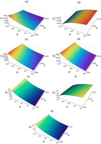
Figure 1 exhibits the variations of different nondimensional coefficients of dispersive and nonlinear terms of a new NLSE given by equation (3.5) as functions of u and $\kappa $ . From this figure, it is found that both uniform current and surface tension have a considerable effect on these coefficients.

Figure 1

Dimensionless coefficients of a new NLSE as functions of u and $\kappa $ .

4 Modulational instability analysis and results

A solution of the coupled nonlinear Schrödinger equations is given by

$$ \begin{align*} \alpha=\frac{\alpha_0}{2}\exp{(-i\Delta\sigma{t})}, \quad \overline\phi=\phi_0, \end{align*} $$

where $\alpha _0$ and $\phi _0$ are real constants and the frequency shift is

$$ \begin{align*} \Delta\sigma=\frac{\mu_1}{4}\alpha_0^2. \end{align*} $$

We assume the perturbation on this solution as follows:

(4.1) $$ \begin{align} \alpha=\frac{\alpha_0}{2}(1+\alpha^{\prime})\exp\{{i(\theta^{\prime}-\Delta\sigma{t})}\},\quad \overline{\phi}=\phi_0+\phi^{\prime}, \end{align} $$

where $\alpha ^{\prime },\theta ^{\prime }$ are small real perturbations of amplitude and phase, respectively, and $\phi ^{\prime }$ is a real small perturbation of $\overline {\phi }$ . Inserting equation (4.1) in equation (3.5), the linearized version of this equation can be simplified to

(4.2) $$ \begin{align} R_1\alpha^{\prime}+R_2\theta^{\prime}-\frac{(\mu_2+\mu_3)}{4}\alpha_0^{2}\frac{\partial\alpha^{\prime}}{\partial{x}}=0 \quad \text{at}~z=0, \end{align} $$

(4.3) $$ \begin{align} R_2\alpha^{\prime}-R_1\theta^{\prime}-\frac{\mu_1}{2}\alpha_0^{2}\alpha^{\prime}+\frac{(\mu_2-\mu_3)}{4}\alpha_0^{2}\frac{\partial\theta^{\prime}}{\partial{x}}-\frac{\partial\phi^{\prime}}{\partial{x}}=0 \quad \text{at}~z=0, \end{align} $$

where

$$ \begin{align*} R_1&=\frac{\partial}{\partial{t}}+c_g\frac{\partial}{\partial{x}}+\gamma_3\frac{\partial^{3}}{\partial{x^{3}}}+\gamma_4\frac{\partial^{3}}{\partial{x}\partial{y^{2}}}+\gamma_8\frac{\partial^{5}}{\partial{x^5}}+\gamma_9\frac{\partial^{5}}{\partial{x^3}\partial{y^2}}+\gamma_{10}\frac{\partial^{5}}{\partial{x}\partial{y^4}}, \\ R_2&=-\gamma_1\frac{\partial^{2}}{\partial{x^{2}}}+\gamma_2\frac{\partial^{2}}{\partial{y^{2}}}+\gamma_5\frac{\partial^{4}}{\partial{x^4}}+\gamma_6\frac{\partial^{4}}{\partial{x^2}\partial{y^2}}+\gamma_7\frac{\partial^{4}}{\partial{y^4}}. \end{align*} $$

The linearized version of equation (3.6) can be expressed as

(4.4) $$ \begin{align} \frac{\partial{\phi^{\prime}}}{\partial{z}}=\alpha_0^{2}\frac{\partial\alpha^{\prime}}{\partial{x}} \quad \text{at}~z=0. \end{align} $$

From equations (3.7) and (4.1), we also have

(4.5) $$ \begin{align} \frac{\partial{\phi^{\prime}}}{\partial{z}}=0 \quad \text{at}~z=-d. \end{align} $$

Now using equation (4.5), we take the plane wave solution of the above equations (4.2), (4.3) and (4.4) given by

$$ \begin{align*} \begin{aligned} \begin{pmatrix} \alpha^{\prime}\\ \theta^{\prime} \end{pmatrix} & = \begin{pmatrix} \hat\alpha\\ \hat\theta \end{pmatrix} \exp\{i(\lambda{x}+\mu{y}-\Omega{t})\}+c.c. , \\ \phi^{\prime}&=\hat{\phi}[\exp\{i(\lambda{x}+\mu{y}-\Omega{t})\}+c.c.]\frac{\cosh{\overline{k}(z+d)}}{\cosh(\overline{k}d)}, \end{aligned} \end{align*} $$

where $\overline {k}^{2}=\lambda ^{2}+\mu ^{2}$ .

The perturbed wavenumbers $\lambda $ , $\mu $ and the perturbed frequency $\Omega $ satisfy the nonlinear dispersion relation

(4.6) $$ \begin{align} \bigg[\overline{R}_1+\frac{(\mu_2+\mu_3)}{4}\alpha_0^{2}\lambda\bigg]\bigg[\overline{R}_1+\frac{(\mu_2-\mu_3)}{4}\alpha_0^{2}\lambda\bigg]=\overline{R}_2\bigg[\overline{R}_2-\frac{\mu_1}{2}\alpha_0^{2}+\frac{\alpha_0^{2}\lambda^2}{\overline{k}\tanh(\overline{k}d)}\bigg], \end{align} $$

where

(4.7) $$ \begin{align} \overline{R}_1&=\Omega-c_g\lambda+\gamma_3\lambda^{3}+\gamma_4\lambda\mu^{2}-\gamma_8\lambda^{5}-\gamma_9\lambda^{3}\mu^{2}-\gamma_{10}\lambda\mu^{4}, \end{align} $$

(4.8) $$ \begin{align} \ \overline{R}_2&=\gamma_1\lambda^{2}-\gamma_2\mu^{2}+\gamma_5\lambda^{4}+\gamma_6\lambda^{2}\mu^{2}+\gamma_7\mu^{4}.\qquad\qquad\qquad \end{align} $$

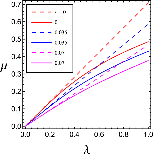
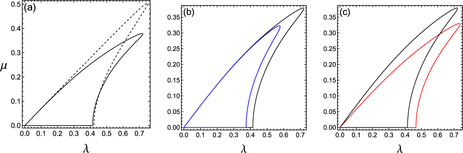
A salient feature of the new broader-banded equation is that the neutral stability curves, as displayed in Figure 2, in the limit $\alpha _0=0$ are no longer straight lines. Note that the fourth-order NLEE corresponding to narrow bandwidth has neutral stability along the intersecting straight lines $\gamma _1\lambda ^{2}-\gamma _2\mu ^{2}=0$ (obtained from equation (4.16)) for $\alpha _0=0$ . In the new broader-banded theory, the corresponding neutral stability curves are obtained from $\overline {R}_2=0$ given by equation (4.8), which agree fairly well with the exact curves of Phillips [Reference Phillips23] for large depth and moderate values of $\lambda $ , $\mu $ .

Figure 2

The stability curves in the limit $\alpha _0=0$ in the $(\lambda ,\mu )$ plane for $u=0$ and several values of $\kappa $ . Solid lines show the new broader-banded results, dashed lines show the narrow-banded results.

The solution of equation (4.6) is given by

(4.9) $$ \begin{align} \overline{R}_1=-\frac{\mu_2}{4}\alpha_0^{2}\lambda\pm\sqrt{{\overline{R}_2\bigg[\overline{R}_2-\frac{\mu_1}{2}\alpha_0^{2}+\frac{\alpha_0^{2}\lambda^{2}}{\overline{k}\tanh(\overline{k}d)}\bigg]+\frac{\mu_3^{2}}{16}}\alpha_0^{4}\lambda^{2}}. \end{align} $$

Using equation (4.7), we can write equation (4.9) as

(4.10) $$ \begin{align} \Omega&=c_g\lambda-\gamma_3\lambda^{3}-\gamma_4\lambda\mu^{2}+\gamma_8\lambda^{5}+\gamma_9\lambda^{3}\mu^{2}+\gamma_{10}\lambda\mu^{4}-\frac{\mu_2}{4}\alpha_0^{2}\lambda \nonumber \\ &\quad \pm \sqrt{{\overline{R}_2\bigg[\overline{R}_2-\frac{\mu_1}{2}\alpha_0^{2}+\frac{\alpha_0^{2}\lambda^{2}}{\overline{k}\tanh(\overline{k}d)}\bigg]+\frac{\mu_3^{2}}{16}}\alpha_0^{4}\lambda^{2}}. \end{align} $$

From equation (4.10), the instability occurs if

(4.11) $$ \begin{align} {\overline{R}_2\bigg[\overline{R}_2-\frac{\mu_1}{2}\alpha_0^{2}+\frac{\alpha_0^{2}\lambda^{2}}{\overline{k}\tanh(\overline{k}d)}\bigg]+\frac{\mu_3^{2}}{16}}\alpha_0^{4}\lambda^{2}<0. \end{align} $$

If the condition in equation (4.11) is satisfied, the perturbed frequency $\Omega $ will be complex valued, and the growth rate of instability represented by the imaginary part $\Omega _i$ of $\Omega $ becomes

(4.12) $$ \begin{align} \Omega_i=\sqrt{{\overline{R}_2\bigg[\frac{\mu_1}{2}\alpha_0^{2}-\overline{R}_2-\frac{\alpha_0^{2}\lambda^{2}}{\overline{k}\tanh(\overline{k}d)}\bigg]-\frac{\mu_3^{2}}{16}}\alpha_0^{4}\lambda^{2}}. \end{align} $$

For $\mu =0$ , the instability condition and the growth rate $\Omega _i$ reduce respectively to

$$ \begin{align*} (\gamma_1\lambda^{2}+\gamma_5\lambda^{4})\bigg[\gamma_1\lambda^{2}+\gamma_5\lambda^{4}-\frac{\mu_1}{2}\alpha_0^{2}+\frac{\alpha_0^{2}|\lambda|}{\tanh(d{\lambda})}\bigg]+\frac{\mu_3^{2}}{16}\alpha_0^{4}\lambda^{2}<0, \end{align*} $$

(4.13) $$ \begin{align} \Omega_i=\sqrt{{(\gamma_1\lambda^{2}+\gamma_5\lambda^{4})\bigg[\frac{\mu_1}{2}\alpha_0^{2}-\gamma_1\lambda^{2}-\gamma_5\lambda^{4}-\frac{\alpha_0^{2}|\lambda|}{\tanh({d\lambda})}\bigg]-\frac{\mu_3^{2}}{16}}\alpha_0^{4}\lambda^{2}}. \end{align} $$

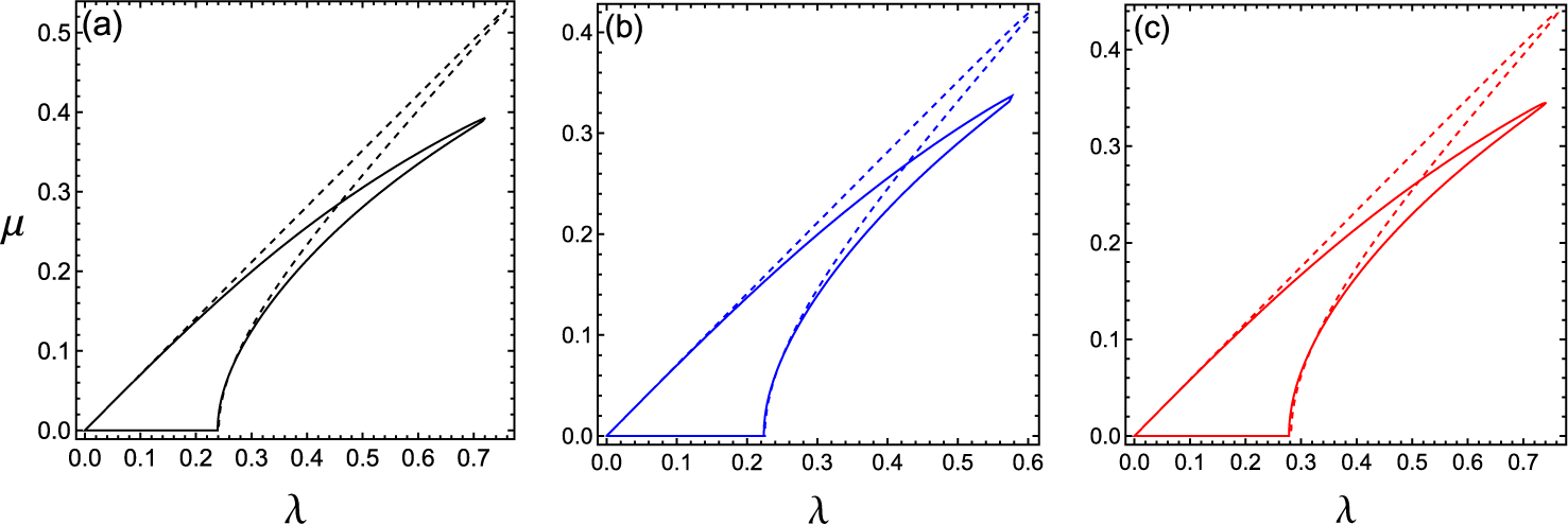
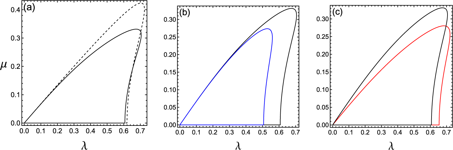
The instability regions obtained from equations (4.11) and (4.17) corresponding to broader bandwidth and narrow bandwidth, respectively, for depth $d=6$ and wave steepness $\alpha _0=0.1$ , $0.2$ , are shown in Figures 3 and 4. Figure 3(a) for $u=0$ , $\kappa =0$ is identical with [Reference Trulsen and Dysthe29, Figure 5]. Thus, we can verify that this limiting case is reproduced properly.

Figure 3

The $(\lambda ,\mu )$ instability diagrams for $d=6$ and $\alpha _0=0.1$ : (a) $u=0,~\kappa =0$ ; (b) $u=0.4,~\kappa =0$ ; (c) $u=0,~\kappa =0.035$ . Solid lines show the new broader-banded result, dashed lines show the narrow-banded result.

Figure 4

The $(\lambda ,\mu )$ instability diagrams for $d=6$ and $\alpha _0=0.2$ : (a) $u=0,~\kappa =0$ ; (b) $u=0.4,~\kappa =0$ ; (c) $u=0,~\kappa =0.035$ . Solid lines show the new broader-banded results, dashed lines show the narrow-banded results.

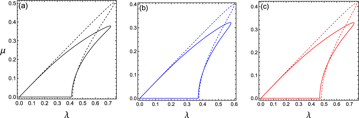
Figures 5 and 6 show the modulational instability regions obtained from equations (4.11) and (4.17) for $\alpha _0=0.2$ and $0.4$ , respectively, in the case of an infinite depth of water. The region bounded by the solid line corresponding to new broader-banded result of Figure 5(a) for $u=0$ , $\kappa =0$ , $\alpha _0=0.2$ is found to nearly overlap with the region obtained from numerical computation of McLean et al. [Reference McLean, Ma, Martin, Saffman and Yuen21, Figure 1(a)]. Therefore, we conclude that the new NLSE for broader bandwidth gives excellent long wavelength two-dimensional instability regions for finite but small wave steepness.

Figure 5

The $(\lambda ,\mu )$ instability diagrams for infinite depth of water and $\alpha _0=0.2$ : (a) $u=0,\kappa =0$ , solid line shows the new broader-banded result, dashed line shows the narrow-banded result. Instability regions for new broader-banded result: (b) $\kappa =0$ , black line shows $u=0$ , blue line shows $u=0.4$ ; (c) $u=0$ , black line shows $\kappa =0$ , red line shows $\kappa =0.035$ . (Colour available online.)

Figure 6

The $(\lambda ,\mu )$ instability diagrams for infinite depth of water and $\alpha _0=0.4$ : (a) $u=0,\kappa =0$ , solid line shows the new broader-banded result, dashed line shows the narrow-banded result. Instability regions for new broader-banded result: (b) $\kappa =0$ , black line shows $u=0$ , blue line shows $u=0.4$ ; (c) $u=0$ , black line shows $\kappa =0$ , red line shows $\kappa =0.035$ . (Colour available online.)

From these figures, we have observed a significant change of the instability regions obtained from broader-banded and narrow-banded results. It is also found that both depth-uniform current and surface tension have a small effect on the instability regions. Furthermore, the instability regions become wider with the increase of $\alpha _0$ .

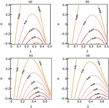
In Figure 7, the contour plots of the growth rate of modulational instability $\Omega _i$ given by equation (4.13) in the $(\lambda ,u)$ plane have been plotted for $d=6$ and two values of $\kappa $ and $\alpha _0$ . We observe that the depth-uniform adverse current increases the growth rate, whereas the following current decreases the growth rate. Further, the growth rate increases with the increase of wave steepness. It is also found that the effect of capillarity is to decrease the growth rate giving a stabilizing influence.

Figure 7

Contour plots of growth rate $\Omega _i(\lambda ,u)$ for $d=6.~\alpha _0=0.2$ : (a) $\kappa =0$ ; (b) $\kappa =0.035$ . $\alpha _0=0.4$ : (c) $\kappa =0$ ; (d) $\kappa =0.035$ .

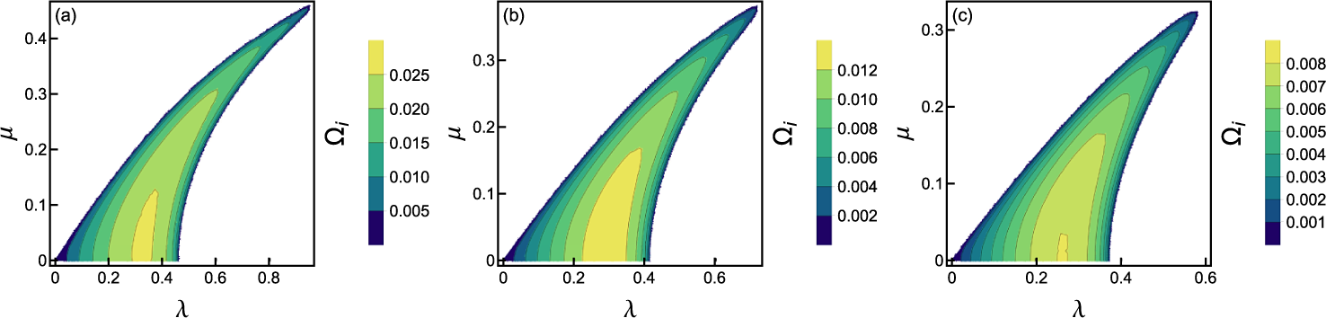
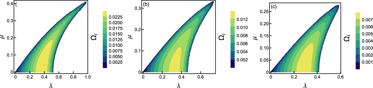
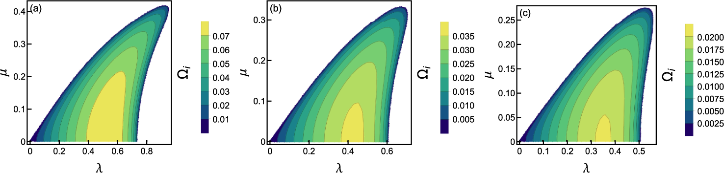
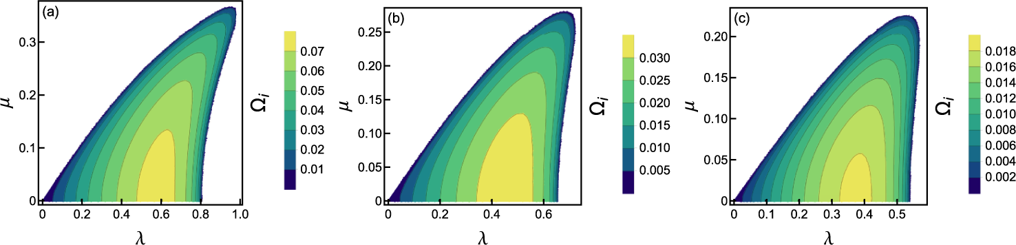
Figures 8–11 show contour plots of instability growth rate $\Omega _i$ given by equation (4.12) in the $(\lambda ,\mu )$ plane for $d=6$ and several values of u, $\kappa $ and $\alpha _0$ corresponding to the new broader-banded result. We have shown that the growth rate decreases with the increase of both u and $\kappa $ , whereas it increases with the increase of $\alpha _0$ . Further, depth-uniform opposing current increases the growth rate. We have also noticed a small change in the shape and span of the contour plots along both the axes.

Figure 8

Contour plots of growth rate $\Omega _i(\lambda ,\mu )$ corresponding to new broader-banded result for $d=6$ , $\alpha _0=0.2$ , $\kappa =0$ : (a) $u=-0.4$ ; (b) $u=0$ ; (c) $u=0.4$ .

Figure 9

Contour plots of growth rate $\Omega _i(\lambda ,\mu )$ corresponding to new broader-banded result for $d=6$ , $\alpha _0=0.2$ , $\kappa =0.035$ : (a) $u=-0.4$ ; (b) $u=0$ ; (c) $u=0.4$ .

Figure 10

Contour plots of growth rate $\Omega _i(\lambda ,\mu )$ corresponding to new broader-banded result for $d=6$ , $\alpha _0=0.4$ , $\kappa =0$ : (a) $u=-0.4$ ; (b) $u=0$ ; (c) $u=0.4$ .

Figure 11

Contour plots of growth rate $\Omega _i(\lambda ,\mu )$ corresponding to new broader-banded result for $d=6$ , $\alpha _0=0.4$ , $\kappa =0.035$ : (a) $u=-0.4$ ; (b) $u=0$ ; (c) $u=0.4$ .

Results for fourth-order NLEE on deep water corresponding to narrow bandwidth may be obtained from equation (3.5) by ignoring the fourth- and fifth-order derivative terms and are given by

(4.14) $$ \begin{align} \Omega=c_g\lambda-\gamma_3\lambda^{3}-\gamma_4\lambda\mu^{2}-\frac{\mu_2}{4}\alpha_0^{2}\lambda\pm\sqrt{P}, \end{align} $$

where

(4.15) $$ \begin{align} P&={\overline{S}\bigg[\overline{S}-\frac{\mu_1}{2}\alpha_0^{2}+\frac{\alpha_0^{2}\lambda^{2}}{\overline{k}\tanh(\overline{k}d)}\bigg]+\frac{\mu_3^{2}}{16}}\alpha_0^{4}\lambda^{2}, \end{align} $$

(4.16) $$ \begin{align} \ \ \overline{S}&=\gamma_1\lambda^2-\gamma_2\mu^2.\qquad\qquad\qquad\qquad\qquad \end{align} $$

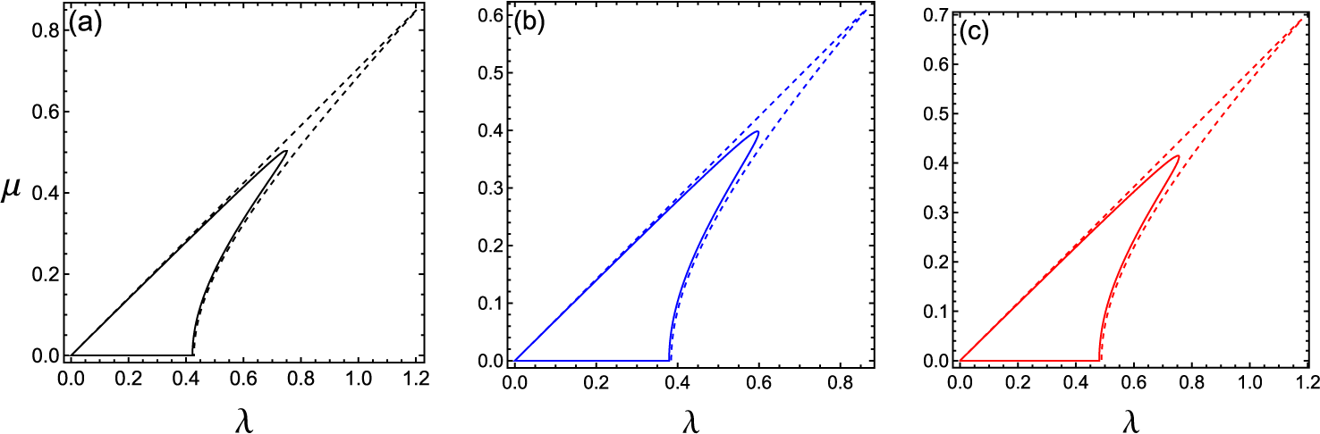
It is important to note that in equation (4.15), the last term $(\mu _3^{2}\alpha _0^{4}\lambda ^{2})/16$ corresponding to the nonlinear term $i\mu _3\alpha ^{2}(\partial \alpha ^{*}/\partial {x})$ of equation (3.5) is insignificant within the fourth-order $O(\epsilon ^{4})$ , and has been often neglected in preceding works [Reference Dhar and Das7, Reference Dysthe10]. However, the actual behaviour of the evolution equation corresponding to narrow bandwidth is described by the full expression of equation (4.15). Considering the last term in equation (4.15) according to Trulsen and Dysthe [Reference Trulsen and Dysthe29], we have observed that its effect is to reduce the extent of the instability region, as shown in Figure 12. As a check, the primary instability regions we obtain in Figure 12(a) for $u=0$ , $\kappa =0$ are compared with those obtained by Trulsen and Dysthe [Reference Trulsen and Dysthe29, Figure 1]. Thus, we can verify that the limiting case is reproduced exactly. Moreover, importance has been attached to the nonlinear term $i\mu _2|\alpha |^2(\partial \alpha /\partial {x})$ of the NLSE in equation (3.5). We find from equation (4.14) that it provides the real $O(\alpha _0^{2})$ correction to the frequency of sufficiently large plane wave perturbations.

Figure 12

The $(\lambda ,\mu )$ instability diagrams for infinite depth and $\alpha _0=0.2$ : (a) $u=0,~\kappa =0$ ; (b) $u=0.4,~\kappa =0$ ; (c) $u=0,~\kappa =0.035$ . Solid lines are based on the full expression of equation (4.15), dashed lines are based on the expression in equation (4.15) excluding the last term.

From equation (4.14), the instability occurs if

(4.17) $$ \begin{align} {\overline{S}\bigg[\overline{S}-\frac{\mu_1}{2}\alpha_0^{2}+\frac{\alpha_0^{2}\lambda^{2}}{\overline{k}\tanh(\overline{k}d)}\bigg]+\frac{\mu_3^{2}}{16}}\alpha_0^{4}\lambda^{2}<0. \end{align} $$

If the condition in equation (4.17) is satisfied, the perturbed frequency $\Omega $ will be complex valued and the growth rate of instability represented by the imaginary part $\Omega _i$ of $\Omega $ becomes

(4.18) $$ \begin{align} \Omega_i=\sqrt{{\overline{S}\bigg[\frac{\mu_1}{2}\alpha_0^{2}-\overline{S}-\frac{\alpha_0^{2}\lambda^{2}}{\overline{k}\tanh(\overline{k}d)}\bigg]-\frac{\mu_3^{2}}{16}}\alpha_0^{4}\lambda^{2}}. \end{align} $$

In the case of one-dimensional perturbation $\mu =0$ , equations (4.17) and (4.18) reduce respectively to

(4.19) $$ \begin{align} {\gamma_1\bigg[\gamma_1\lambda^{2}-\frac{\mu_1}{2}\alpha_0^{2}+\frac{\alpha_0^{2}|\lambda|}{\tanh({d\lambda})}\bigg]+\frac{\mu_3^{2}}{16}}\alpha_0^{4}<0, \end{align} $$

(4.20) $$ \begin{align} \Omega_i=\lambda~\sqrt{{\gamma_1\bigg[\frac{\mu_1}{2}\alpha_0^{2}-\gamma_1\lambda^{2}-\frac{\alpha_0^{2}|\lambda|}{\tanh({d\lambda})}\bigg]-\frac{\mu_3^{2}}{16}}\alpha_0^{4}}. \end{align} $$

Omitting last term of equation (4.19), it becomes

(4.21) $$ \begin{align} \gamma_1^{2}\lambda^{2}-\frac{\gamma_1}{2}\bigg[\mu_1-\frac{2|\lambda|}{\tanh({d\lambda})}\bigg]\alpha_0^{2}<0. \end{align} $$

Note that in the absence of depth-uniform current, instability is possible when

$$ \begin{align*} (2\kappa-1)(3\kappa^{2}+6\kappa-1)>0, \end{align*} $$

from which the ranges of $\kappa $ are given by

$$ \begin{align*} 0<\kappa<(2/\sqrt{3}-1)=0.1547, \quad 0.5<\kappa<\infty. \end{align*} $$

These results are in agreement with the results obtained by Zakharov [Reference Zakharov32]. Herein, the value 0.1547 of $\kappa $ corresponds to the minimum group velocity and the value 0.5 of $\kappa $ to the first Wilton [Reference Wilton31] ripple.

For infinite depth, the expression for maximum growth rate of instability becomes

(4.22) $$ \begin{align} G_m=\frac{|\mu_1|}{4}\bigg[1-\frac{1}{\mu_1}\bigg(\frac{\mu_1}{\gamma_1}\bigg)^{\frac{1}{2}}\alpha_0\bigg]\alpha_0^{2}, \end{align} $$

which occurs for the wavenumber

$$ \begin{align*} \lambda_m=\frac{1}{2}\bigg[\sqrt{\frac{\mu_1}{\gamma_1}}-\frac{3}{4\gamma_1}\alpha_0\bigg]\alpha_0. \end{align*} $$

For $u=0$ , $G_m$ takes the form

(4.23) $$ \begin{align} G_m=\frac{1}{16}\bigg[1+\frac{8}{\sqrt{6}}\alpha_0\bigg]\alpha_0^{2} \end{align} $$

in the case of pure capillary waves, and reduces to

(4.24) $$ \begin{align} G_m=\tfrac{1}{2}\big[1+\tfrac{9}{8}\kappa-2\big(1+\tfrac{73}{16}\kappa\big)\alpha_0 \big]\alpha_0^{2}, \end{align} $$

when $\kappa $ is small.

The expressions for $G_m$ given by equations (4.23) and (4.24) are identical with Hogan’s [Reference Hogan14, equations (3.16b) and (3.16c)], respectively. It is important to note that the correction to the maximum growth rate in equation (4.22) is of fourth-order, involving three terms, namely, the frequency-dispersion term, the nonlinear term and the mean flow term. Since the frequency-dispersion term for pure capillary waves is of opposite sign of pure gravity waves, so too are the corrections to the stability properties.

From equation (4.21), the instability bandwidth for infinite depth is given by

$$ \begin{align*} \lambda=\bigg[\sqrt{\frac{\mu_1}{2\gamma_1}}-\frac{1}{2\gamma_1}\alpha_0\bigg]\alpha_0. \end{align*} $$

At marginal stability, $\Omega _r$ , the real part of $\Omega $ then becomes

(4.25) $$ \begin{align} \Omega_r=c_g\bigg[\sqrt{\frac{\mu_1}{2\gamma_1}}-\frac{1}{2\gamma_1}\alpha_0\bigg]\alpha_0. \end{align} $$

Further, the value of the real part of $\Omega $ corresponding to $\lambda _m$ is

(4.26) $$ \begin{align} \Omega_{rm}=\frac{c_g}{2}\bigg[\sqrt{\frac{\mu_1}{\gamma_1}}-\frac{3}{4\gamma_1}\alpha_0\bigg]\alpha_0. \end{align} $$

Result for the third-order Schrödinger equation analysis on infinite depth has been given previously by Liao et al. [Reference Liao, Dong, Ma and Gao17] for $\Omega =0$ , and may be obtained from equation (4.20) by omitting the fourth-order terms and setting $\kappa = 0$ , and it is given by

(4.27) $$ \begin{align} \frac{\Omega_i}{\alpha_0^{2}}=\frac{\lambda}{\alpha_0}\sqrt{\frac{\gamma_1\mu_1}{2}-\gamma_1^{2}\bigg(\frac{\lambda}{\alpha_0}\bigg)^{2}}. \end{align} $$

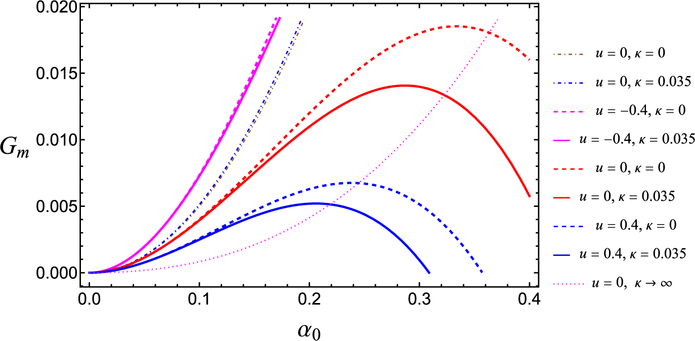
The maximum growth rate of instability $G_m$ given by equation (4.22) is shown in Figure 13 as a function of wave steepness $\alpha _0$ for some values of u and $\kappa $ . For $u=0$ , $\kappa =0$ , the red dashed curve obtained from the fourth-order result nearly overlaps with the curve for class I, $m=1$ of McLean [Reference McLean20, Figure 6]. So we find an excellent agreement with the exact numerical result of McLean [Reference McLean20]. As described by McLean, the class I, $m=1$ instability has a growth rate of second-order of wave steepness for small wave steepness, which is in agreement with the perturbation analysis of Benjamin and Feir [Reference Benjamin and Feir1]. It is also seen from Figure 13 that the maximum growth rate obtained from the fourth-order result first increases with $\alpha _0$ and then decreases, while the growth rate $G_m$ computed from the third-order result (shown as dash–dotted line) increases steadily with $\alpha _0$ . The depth-uniform following current first increases and then decreases the modulational instability, whereas an opposing current significantly increases the growth rate. In the absence of depth-uniform current, we observe a significant change of the maximum growth rate obtained from equations (4.23) and (4.24) for pure capillary waves ( $\kappa \rightarrow \infty $ , shown as a dotted line) and pure gravity waves ( $\kappa =0$ , shown as a red dashed line), respectively, due to the sign change of the frequency-dispersion term. Further, the effect of surface tension is to decrease the growth rate of instability.

Figure 13

Plot of $G_m$ versus $\alpha _0$ for several values of u and $\kappa $ . Solid, dashed and dotted lines show the fourth-order results, dash–dotted lines show the third-order results.

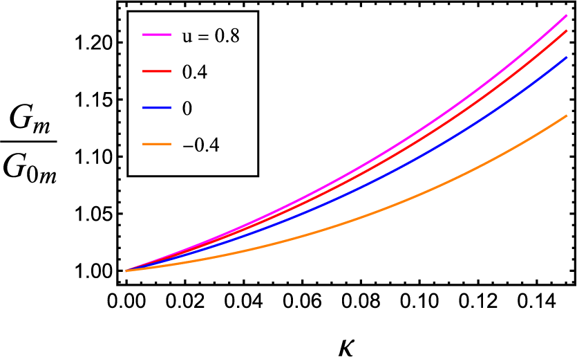
In Figure 14, the ratio of the maximum growth rate of instability to its value in the absence of capillarity corresponding to the third-order result obtained from equation (4.22) has been plotted against $\kappa $ for different values of depth-uniform current u. We observe that the effects of both capillarity and depth-uniform current are to increase steadily the maximum growth rate.

Figure 14

Normalized maximum growth rate versus $\kappa $ for some values of u.

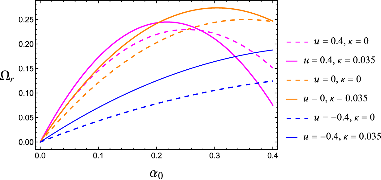
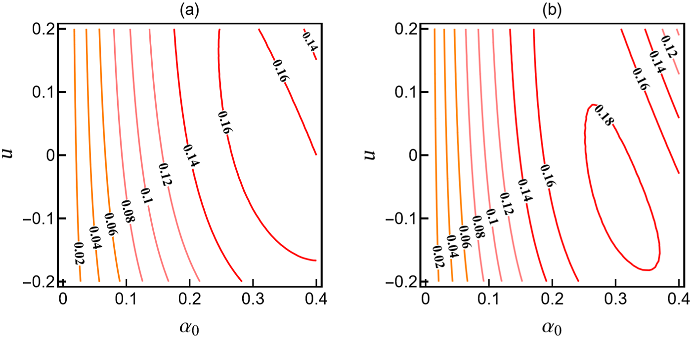
The perturbed frequency $\Omega _r$ at marginal stability given by equation (4.25) has been plotted in Figure 15 against $\alpha _0$ for different values of u and $\kappa $ . For $u = 0$ , $\kappa = 0$ , it is observed that equation (4.25) is fairly close to the exact results of Longuet-Higgins [Reference Longuet-Higgins18] for $\alpha _0 < 0.3$ . In Figure 16, the contour plots of $\Omega _{rm}(\alpha _0,u)$ given by equation (4.26) have been plotted for two values of $\kappa $ .

Figure 15

Curves of marginal stability versus $\alpha _0$ for some values of u and $\kappa $ .

Figure 16

Contour plots of frequency separation of fastest growing sideband $\Omega _{rm}(\alpha _0,u)$ : (a) $\kappa =0$ ; (b) $\kappa =0.035$ .

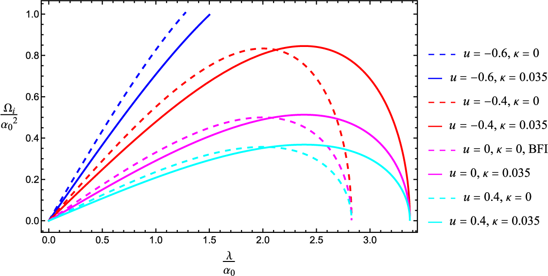
Figure 17 shows the growth rate $\Omega _i/\alpha _0^{2}$ given by equation (4.27) as a function of $\lambda /\alpha _0$ at different values of u and $\kappa $ . We find that the depth-uniform adverse current can largely expand the onset criterion and significantly enhances the instability growth rate, whereas the depth-uniform following current decreases the growth rate, consistent with the result of Liao et al. [Reference Liao, Dong, Ma and Gao17]. Furthermore, the influence of the capillary is to depress the instability growth rate due to modulation.

Figure 17

Plot of growth rate of instability $\Omega _i/\alpha _0^{2}$ versus $\lambda /\alpha _0$ for several values of u and $\kappa $ . BFI refers to the Benjamin–Feir instability.