







1. Introduction
Gravity current (GC) is a generic name for the flow of a thin layer of fluid into another fluid (the ambient) of a different density. The flow is over/under a horizontal or down-slope/up-slope boundary. The density difference is due, typically, to (a) temperature or composition (e.g. cold air in warm air, or saline in fresh water), and (b) the presence of small suspended particles or drops, which form the particle-driven or turbidity GC. The understanding of turbidity currents has application in geophysical and environmental situations, like the transport of silt, avalanches, volcanic pyroclastic flows and clouds and safety of submarine structures. A review of the state of knowledge (e.g. Ungarish Reference Ungarish2020 referred below as U20) reveals that the initial (slumping phase) propagation of a lock-release gravity GC over a down slope has received little attention, in particular when the driving force is due to suspended particles (turbidity currents). The gaps of knowledge have been emphasized by the recent experimental studies of GMRL and HHLWG for GCs over slopes  $\gamma$ of up to approximately
 $10^\circ$; the lock of length
 $x_0$ and height
 $h_0$ was filled with a dilute suspension of dense particles which settle during the propagation (figure 1). Hereafter, we use the following abbreviation for literature references: D13 = Dai (Reference Dai2013), GMRL = Gadal et al. (Reference Gadal, Mercier, Rastello and Lacaze2023), HHLWG = Han et al. (Reference Han, He, Lin, Wang, Guo and Yuan2023), M10 = Maxworthy (Reference Maxworthy2010), U20 = Ungarish (Reference Ungarish2020).
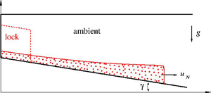
Sketch of the systems (a) without ramp  $x_{slope} =0$, and (b) with ramp
 $x_{slope} =x_0$. The GC is initially (
 $t=0$) in the lock (dashed line) of dimensions
 $x_0, h_0$. (In realistic laboratory systems the lock in configuration (a) is slightly different, such as box or a horizontal top interface. We ignore this detail.)

The work in GMRL concluded, empirically, that, for a sufficiently small settling velocity of the dispersed particles, the inclined particle-driven GC behaves like the classical counterpart, i.e. the simple case of a homogeneous fluid (saline) released from a rectangular lock over a horizontal bottom (much longer than the lock) into a homogeneous ambient fluid (fresh water) of constant height, at a large Reynolds number. This classical GC displays a constant  $u_N$ (speed of propagation) for a significant slumping time (and length) interval, as recorded by experiments and predicted by a simplified theory (e.g. Rottman & Simpson Reference Rottman and Simpson1983; Ungarish Reference Ungarish2020). The theoretical interpretation, and modelling, of these observation of GMRL is deficient. Some experimental studies for GCs on a slope (e.g. M10 and D13) attempted to match the data with the propagation formula of the ‘thermal theory’ (Beghin, Hopfinger & Britter Reference Beghin, Hopfinger and Britter1981). This approximation models the dense fluid as a box of oval shape, and is rather a descriptive (not predictive) tool, reliant on adjustable constants that must be determined empirically. Moreover, this model suggests a
 $t^{-1/3}$ decay of
 $u_N$ for most of the slumping interval, in clear-cut contrast with the insights of GMRL (details will be presented latter). A reliable interpretation of the main conclusions of GMRL requires a sharper theoretical tool. The best candidate is the shallow-water (SW) theory, that performs well for a large class of GCs in horizontal propagation; see U20. This motivated the present work whose main objective is the use of an appropriate SW model for the analysis of the configurations under consideration. This includes the formulation, solutions and comparisons with the available data.
Some previous works in these directions, for composite GCs on a slope, have been published before. The book U20 section 11.2 presented a SW one-layer formulation (no return flow in the ambient above the GC) and Zemach et al. (Reference Zemach, Ungarish, Martin and Negretti2019) presented a two-layer counterpart (but without entrainment and drag). These models must be significantly modified for the present problem. The significant data are for full-depth (or close to it) lock release, and hence the proper physical model is a two-layer formulation, with entrainment and drag. Moreover, since we focus on particle-driven GCs, it is essential to incorporate this effect into the SW formulation.
The SW classical GC has constant density (i.e. zero entrainment and no particle settling), propagates in a horizontal channel of constant height and encounters no drag. The driving effect is the constant reduced gravity, and the reaction of the fluid is inertial acceleration. The extended SW GC, which is considered in this study, is affected by what we call ‘source terms’ (‘source’ is a generic name for the non-homogeneous terms in the governing balance differential equations, and physically this includes a ‘sink’ when the contribution is negative). In the extended formulation the source (sink) of volume and mass of the GC (and hence of density) is caused by particle settling and entrainment, and the source (sink) of momentum is contributed by the slope and drag. However, in many cases of interest the source terms are relatively small as compared with the main contributors to the governing balances of volume, mass and momentum. Consequently, the insights and results provided by the classical GC (zero source terms) are useful references and guidelines for the extended analysis.
The structure of the paper is as follows. Section 2 gives the formulation of the SW governing equations and boundary conditions, and a short discussion of the slumping concept. Results of the SW theory and comparisons with experimental data are presented in § 3. First, in § 3.1, we focus attention on configurations close to these of GMRL: we discuss the effects of the settling speed dimensionless parameter  $\beta$, aspect ratio
 $(x_0/h_0)$, slope
 $\gamma$ and the depth of the ambient. Then, we consider the system of HHLWG in § 3.2 with fixed
 $\gamma = 9^\circ$,
 $(x_0/h_0) = 2.1$, and particles with two settling speeds. Finally, in § 3.3 we consider some systems of compositional GCs; for these cases, data for long propagation (after the slumping phase) are available for comparisons. Concluding remarks are presented in § 4. Appendices A and B clarify the front-jump condition used in the SW formulation, and the associated effect of the open top on the result. A list of abbreviations is given next.
2. Formulation
2.1. The governing equations
We use dimensional variables unless stated otherwise. The variables of the ambient fluid are denoted by the subscript  $a$, while these of the current are without subscript (or with subscript
 $c$ when emphasis is needed). We use the Cartesian
 $xz$ two-dimensional system with
 $x$ horizontal and
 $z$ vertically upward, and corresponding
 $u,w$ velocity components. Gravity
 $g$ acts in the -
 $z$ direction. The geometry is as follows (figure 1). The top and bottom of the channel are at
 $z=z_T = {\rm const.}$ and
 $z_B(x)$. The height and slope of the channel are
 \begin{equation} H = H(x) = z_T - z_B(x), \quad \gamma = \gamma(x) ={-} \frac{ {\rm d} z_B}{{\rm d} x}. \end{equation}
For simplicity, and in accord with the laboratory systems relevant to this paper, we assume that  $\gamma = 0$ for
 $x< x_{slope}$ (a ramp, if present) and a constant for larger
 $x$. The lock is defined by the backwall
 $x=0$, dam (gate) at
 $x=x_0$ and is of height
 $h_0$ above the bottom. We shall assume a constant
 $h_0$ (although this is slightly inconsistent with some practical systems. When
 $x_{slope} = 0$ the interface of the lock may be horizontal, or a rigid wall of a box).
The ambient fluid is of constant density  $\rho _{a}$. The current is a suspension of particles of radius
 $a_p$ and density
 $\rho _p> \rho _{a}$ that occupy a volume fraction
 $\alpha$ (initially
 $\alpha _0$); the density of the interstitial fluid is
 $\rho _{a}$ (same as that of the ambient). Therefore, the density of the GC is
 \begin{equation} \rho_{c} = \rho_{a} + \alpha (\rho_p - \rho_{a}). \end{equation}
We shall assume that the suspension is dilute (i.e.  $\alpha _0 \ll 1$) and the system is Boussinesq (abbreviated as Bq), i.e.
 $\alpha _0 (\rho _p - \rho _{a})/\rho _{a} \ll 1$. The settling speed of the particles
 $W_S$ is known, either by measurement, or by the Stokes formula
 \begin{equation} W_S = (2/9) (\rho_p/\rho_{a} -1) g a_p^2/\nu, \end{equation}
where  $\nu$ is the kinematic viscosity of the fluid.
We introduce the initial reduced gravity
 \begin{equation} g' = \alpha(0) \frac{\rho_p - \rho_{a}}{\rho_{a}} g. \end{equation}
The balance SW equations consider a quite general system; see U20. Since the GC is a thin layer, attention is focused on the longitudinal behaviour, for depth-averaged  $u(x,t), u_a(x,t)$ and
 $\alpha (x,t)$, where
 $t$ is the time from the release (dam-break) occurrence. We define the scaled volume fraction
 \begin{equation} \phi = \phi(x,t) = \frac{\alpha(x,t)}{\alpha_0}. \end{equation}
Initially,  $\phi = 1$ in the lock, then
 $\phi$ decreases due to settling and entrainment. The effective reduced gravity is
 $\phi g'$.
The thin-layer hypothesis implies  $|w/u| \ll 1$. Consequently, the
 $z$-momentum equation is well approximated by the hydrostatic balance. We note that, for consistency with the
 $|w/u| \ll 1$ assumption, we must also assume that the entrainment coefficient
 $E$ (see below) is small, and the slope angle
 $\gamma$ is not large.
Let  $q = u h$,
 $\tilde {u} = u-u_a$. The global continuity in the channel yields
 \begin{equation} q_a = u_a (H - h) ={-}q, \quad u_a ={-}q /(H - h). \end{equation}
The volume continuity equation of the current is
 \begin{equation} \frac{\partial h}{\partial t} +\frac{\partial q}{\partial x} = E |\tilde{u}|, \end{equation}
where  $E$ is a dimensionless entrainment coefficient (to be specified later). The particle (dispersed phase) balance is
 \begin{equation} \frac{\partial \alpha h }{\partial t} +\frac{\partial \alpha q }{\partial x} ={-}W_S \alpha. \end{equation}
The momentum equations need some manipulations. The  $z$-pressure balance is hydrostatic,
 $\partial p_k /\partial z = -(\rho _k - \rho _{a}) g, \ (k = a,c)$, where
 $p$ is the reduced pressure (upon addition of
 $\rho _{a} g z$). Consequently,
 $p_a = p_a(x,t)$, a
 $z$-independent function. The pressure is continuous,
 $p_c(x,t,z) = p_a(x,t)$, at the interface
 $z = z_B(x) + h(x,t)$. The shear and turbulent stresses are neglected (which implies free-slip top and bottom boundaries). The depth-averaged
 $x$-momentum equations for the layers of ambient and suspension (current) are expressed as
 $$\begin{gather} \frac{\partial \rho_{a} q_a }{\partial t} + \frac{\partial }{\partial x} \frac{\rho_{a} q_a^2}{H - h} ={-}(H - h) \frac{\partial p_a }{\partial x} + D, \end{gather}$$
 $$\begin{gather}\frac{\partial \rho_{c} q }{\partial t} +\frac{\partial }{\partial x} \frac{\rho_{c} q^2}{h} ={-} h \frac{\partial p_a }{\partial x} - \rho_{a} g' \frac{\partial}{\partial x} \left(\frac{1}{2} \phi h^2\right) + \rho_{a} g' \tan \gamma \phi h - D, \end{gather}$$
where  $D = \rho _{a} c_D |\tilde {u}| \tilde {u}$ is the interfacial drag and
 $c_D$ is a dimensionless coefficient.
We recall the Bq simplification  $\rho _{a} \approx \rho _{c}$, eliminate
 $\partial p_a/\partial x$ between (2.9) and (2.10) and substitute
 $q_a = -q$. We obtain a partial differential equation (PDE) for
 $q(x,t)$ as follows:
 \begin{equation} \frac{\partial q }{\partial t} + \left (1 - \frac{h}{H}\right ) \frac{\partial}{\partial x} \left ( \frac{q^2}{h} + \frac{1}{2} \mathrm{g}' \phi h^2 \right ) - \frac{h}{H} \frac{\partial}{\partial x} \left ( \frac{q^2}{H -h} \right ) =\left (1 - \frac{h}{H} \right ) S, \end{equation}
where
 \begin{equation} S = \tan \gamma \cdot g' \phi h - \left ( \frac{H}{H-h} \right )^2 c_D u^2 ; \end{equation}
(in the drag term we assume  $u \ge 0$).
We switch to dimensionless variables, defined as follows:  $x$ is scaled with
 $x_0$, heights with
 $h_0$, velocity with
 $U = (g' h_0)^{1/2}$, time with
 $T = x_0/U$ and volume with
 $x_0 h_0$. Since the vertical and horizontal lengths are scaled differently, the aspect ratio of the lock,
 $\lambda = x_0/h_0$ enters into the governing equation (actually, into the source terms). The dimensionless settling speed is
 \begin{equation} \check{\beta} = \frac{W_S}{U}. \end{equation}
The literature (Bonnecaze, Huppert & Lister Reference Bonnecaze, Huppert and Lister1993; U20, GMRL) use the parameter
 \begin{equation} \beta = \frac{W_S}{U} \frac{x_0}{h_0} = \check{\beta} \frac{x_0}{h_0}. \end{equation}
Here,  $\beta$ (called Stokes number in GMRL) is the ratio of two typical time intervals: the propagation of the GC over one lock length and the settling of a particle over the height of the lock. Therefore, we are interested in systems with
 $\beta \ll 1$, otherwise the particles settle out from the suspension before a significant GC develops.
It is also convenient to introduce the variable  $\varphi = \phi h$, which expresses the buoyancy of the GC at the position
 $x$ at time
 $t$. Recall,
 $u = q/h$.
In dimensionless form, the governing equations for the variable  $h, \varphi, q$ read
 $$\begin{gather} \frac{\partial h}{\partial t} +\frac{\partial q}{\partial x} = E \frac{x_0}{h_0} |\tilde{u}|, \end{gather}$$
 $$\begin{gather}\frac{\partial \varphi }{\partial t} +\frac{\partial \varphi u }{\partial x} ={-} \beta \varphi/h, \end{gather}$$
 $$\begin{gather}\frac{\partial q }{\partial t} + \left (1 - \frac{h}{H}\right ) \frac{\partial}{\partial x} \left ( \frac{q^2}{h} + \frac{1}{2} \varphi h \right ) - \frac{h}{H} \frac{\partial}{\partial x} \left ( \frac{q^2}{H -h} \right ) = \left (1 - \frac{h}{H} \right ) S \frac{x_0}{h_0}, \end{gather}$$
where
 \begin{equation} S = \tan \gamma \cdot \varphi - \left ( \frac{1}{1-h/H} \right )^2 c_D u^2. \end{equation}
The terms associated with  $E, c_D, \gamma$ and
 $\beta$ are referred to as ‘source terms’ for obvious reasons; we reiterate that, physically, a negative source is a sink. In practice, we have control (or reliable knowledge) of the values of
 $\gamma$ and
 $\beta$, while
 $E$ and
 $c_D$ are provided by some indirect (and less reliable) estimates of which we have no control. In any case, there is good evidence that
 $E$ and
 $c_D$ are small for typical Bq GCs (Johnson & Hogg Reference Johnson and Hogg2013; Negretti, Flor & Hopfinger Reference Negretti, Flor and Hopfinger2017). Consequently, it is justified to assume that the source terms in our analysis are small (intrinsically and by design), and hence the extended SW solutions will bear qualitative similarities to the classical GCs (zero source terms).
To close the system we need a front-jump condition and correlations for  $c_D$ and
 $E$. For the front condition we use a straightforward extension of the classical GC case, namely
 \begin{equation} u_N = \frac{{\rm d} x_N}{{\rm d} t} = Fr(a) \varphi^{1/2}, \end{equation}
where  $a = h_N/H(x_N)$ at the nose and
 $Fr(a)$ is a standard nose-Froude formula. We shall use the theoretical formula of Benjamin (Reference Benjamin1968) as
 \begin{equation} Fr(a) = [(2-a)(1-a)/(1+a)]^{1/2}. \end{equation}
We recall that  $Fr$ increases from
 $0.71$ to
 $1.4$ as
 $a$ decreases from
 $0.5$ to
 $0$. As shown by Benjamin (Reference Benjamin1968) and confirmed by others (see U20 § 4.3) the front jump is dissipative for
 $a<0.5$ but needs energy supply for
 $a>0.5$, and hence GCs with
 $a>0.5$ are non-physical. The derivation of (2.20) is rigorous for a horizontal channel. We argue, see Appendix A, that (2.19)–(2.20) are a fair approximation for
 $|\gamma | < 15^\circ$ (estimated error <10 %), and are expected to provide acceptable qualitative results up to
 $\gamma \approx 30^\circ$. The along-slope speed of propagation is simply
 $u_N/\cos \gamma$, but since the difference is only 2 %–3 % for most cases discussed in this paper, we shall ignore the
 $1/ \cos \gamma$ correction, and refer to
 $u_N$ and
 $x_N$ as the along-slope values, unless stated otherwise.
The coefficients  $c_D$ and
 $E$ are attributed to interfacial instabilities associated with the bulk Richardson number defined here as (using dimensionless variables)
 \begin{equation} Ri = Ri(x,t) = \frac{\varphi }{\tilde{u}^2} = \frac{\varphi}{u^2} (1 - h/H)^2. \end{equation}
For  $c_D$ we use a constant value, 0.10, unless stated otherwise, for
 $Ri \le 1$ and 0 for
 $Ri >1$; this value is suggested by the experimental data of Negretti et al. (Reference Negretti, Flor and Hopfinger2017), and numerical tests with some different values confirmed its robustness. For entrainment we employ the correlation of Johnson & Hogg (Reference Johnson and Hogg2013) as
 \begin{equation} E = \frac{E_0}{1 + k Ri}, \end{equation}
with  $E_0 = 0.075$,
 $k= 27$. These are empirical correlations with adjustable constants. In this sense, the SW formulation is not self-contained. However,
 $E$ and
 $c_D$ are ‘off the shelf’ inputs, expected to be of broad validity, not some undetermined parameters that should be calibrated again and again for any particular experiments. We shall keep the same
 $E$ and
 $c_D$ for all the comparisons made in this work. We emphasize that the SW model is not restricted to these particular closures for
 $E$ and
 $c_D$, and other correlations can be used when more information becomes available.
The initial conditions are  $h = 1$,
 $u = 0$,
 $\varphi = 1$ in the lock
 $0 \le x <1$,
 $x_N(t = 0) = 1$, and at the backwall
 $x=0$ we impose
 $q(0,t) = 0$.
An inspection of the equations reveals that the analysis of the propagation of the GC stage is in general a complex task. Even under the Bq simplification, the flow is governed by a large number of dimensionless parameters: the slope  $\gamma$, the changing height
 $H(x)$, the entrainment correlation
 $E(Ri)$, the drag coefficient
 $c_D$, the particle settling coefficient
 $\check {\beta }$ and the lock aspect ratio
 $\lambda =(x_0/h_0)$.
2.2. Boundary values
The behaviour of the GC at the endpoints  $x=0$ and
 $x = x_N$ is of interest, and also a needed condition for numerical solutions. Some useful results are provided by (2.15) and (2.16).
For  $x=0$, we impose
 $u= q$ = 0. We obtain
 $$\begin{gather} \frac{{\rm d} h(0,t)}{{\rm d}t} ={-} \frac{\partial q}{\partial x}(x = 0), \end{gather}$$
 $$\begin{gather}\frac{{\rm d} \varphi(0,t)}{{\rm d}t} ={-} \frac{\varphi(0,t)}{h(0,t)} \left [\frac{\partial q}{\partial x}(x = 0) + \beta \right ]. \end{gather}$$
For  $x = x_N(t)$ (a moving point) we first transform the equations of motion from dependency on
 $x,t$ to dependency on
 $\xi, t$ where
 $\xi = x/x_N(t) \in [0,1]$ (see U20), then analyse the behaviour at
 $\xi = 1$. We obtain
 $$\begin{gather} \frac{{\rm d} h_N}{{\rm d}t} ={-} h_N \left.\frac{\partial u}{\partial x}\right|_N + E \frac{x_0}{h_0} u_N, \end{gather}$$
 $$\begin{gather}\frac{{\rm d} \varphi_N}{{\rm d}t} ={-} \varphi_N \left [ \left.\frac{\partial u}{\partial x}\right|_N + \beta \frac{1}{\displaystyle{h_N}} \right ] . \end{gather}$$
2.3. Reductions: compositional GC and one-layer model
The compositional (homogeneous) GC formulation is recovered as follows. We represent the density excess  $\rho _{c}(t=0) - \rho _{a}$, and hence the appropriate
 $g'$, as produced by a suspension of non-settling particles (
 $W_S = 0$). The dimensionless equations of motion, with
 $\beta = 0$, remain valid. In this case, the reduced volume fraction
 $\phi (x,t)$ represents the dilution of
 $\rho _{c}$ due to entrainment,
 $\rho _{c}(x,t) = \rho _{a} + [ \rho _{c}(t=0) - \rho _{a} ] \phi (x,t)$.
The one-layer formulation assumes that there is no return flow in the ambient fluid. Formally, the only change in the system of equations and boundary conditions is the setting  $h/H=0$ in the momentum equation (2.20), source term (2.18) and Richardson number (2.21). The one-layer formulation does not capture and reproduce the internal bores (jumps) of the interface which are predicted by the two-layer formulation for
 $H <2$ (see U20 § 6.4), in accord with experiments (Rottman & Simpson Reference Rottman and Simpson1983). The presence/absence of such bores is an important issue in the slumping phase, as clarified below.
2.4. The slumping-phase concept
The dense fluid in the reservoir (lock) is a stationary bulk, bounded by a horizontal interface and two vertical walls. After the removal of the gate, this fluid is activated into motion, and this is reflected by the change of shape of the interface: it spreads out in front of, and behind, the broken gate. After a while the interface displays a thick front bulk followed by an elongating tail, and eventually the tail reaches the front (nose). The GC spreads out a few lock lengths during this stage. Roughly, this quite general rearrangement can be called ‘slumping’. An interesting feature is that, during this adjustment, the nose displays a special pattern of propagation, in some cases with a small (or zero) deceleration (and this changes strongly after the tail reaches the front). The possibility of propagation with a constant  $u_N$ made the slumping stage the focus of practical and theoretical interest in the study of GCs. For example, the widely cited paper of Huppert & Simpson (Reference Huppert and Simpson1980) used the term ‘slumping’ in an attempt to document systematically and explain theoretically the constant
 $u_N$ observed in homogeneous Bq-system experiments in rectangular cross-section channels. Extensions of this effect, by experiment and theory to (a) non-Bq systems, (b) stratified ambient and (c) non-rectangular cross-section were sought, and reported by (a) Lowe, Rottman & Linden (Reference Lowe, Rottman and Linden2005) and Rotunno et al. (Reference Rotunno, Klemp, Bryan and Muraki2011), (b) Maxworthy et al. (Reference Maxworthy, Leilich, Simpson and Meiburg2002) and Ungarish & Huppert (Reference Ungarish and Huppert2002) and (c) Ungarish, Mériaux & Kurz-Besson (Reference Ungarish, Mériaux and Kurz-Besson2014) and Zemach & Ungarish (Reference Zemach and Ungarish2013).
For a sharp discussion of the slumping phase (or slumping) we introduce several restrictions: we consider release from a rectangular lock (of finite length), and follow the behaviour for a propagation to approximately 5–15 lock lengths. The system is Bq, and not stratified.
The slumping concept has been introduced to emphasize a simple, but not trivial, behaviour: the propagation of the lock-release classical GC with a constant  $u_N$ for a significant distance. This pattern has been suggested by observations and subsequently derived as a rigorous solution of the SW equations for the classical GC. This pattern is robust: it appears for full- and part-depth locks. The classical GC is characterized by a constant
 $H$, and
 $\gamma =E=c_D = \beta =0$. This implies that the source terms on the right-hand side of the governing equations (2.15)–(2.17) are zero. Since the aspect ratio
 $(x_0/h_0)$ enters into the formulation as a coefficient in the source terms, we conclude that the (scaled) SW solution of the classical GC is independent of
 $(x_0/h_0)$. (We keep in mind that this simplification is not valid when one of the parameters
 $\gamma, E, c_D, \beta$ is non-zero.) Upon the lack of the source terms, (2.15) and (2.16) predict
 $\varphi = h$, i.e.
 $\phi =1$ (a straightforward physical consequence when there is no entrainment and no particle sedimentation). Equation (2.16), and the associated boundary conditions (2.24) and (2.26), become redundant. The reduced system (2.15), (2.17) and (2.19) can be expressed as standard set of hyperbolic PDEs for the variables
 $h(x,t)$ and
 $u(x,t)$ with the simple initial conditions
 $h=1, u=0$ in the lock, see U20 § 6.3. The motion that occurs by opening the gate at
 $x=1, t=0$ is a classical dam-break problem which can be solved, analytically, by the method of characteristics. (We extend the term ‘analytical’ to include also simple numerical procedures like the iterative calculation of a root and integration of an ordinary differential equation.)
The rigorous dam-break solution (see U20 §§ 3.3 and 6.3) shows a clear-cut stage of propagation for  $0< t \le t_{slump}$ with constant
 $u_N$ for a significant distance of propagation,
 $x_N(t_{slump}) = x_{slump}$. (Some discussions measure the slumping distance from the gate,
 $x_{slump} -1$.) The values of the slumping
 $u_N$ and
 $x_{slump}$ are functions of
 $H$ only: the first increases (from approximately 0.5 to 0.8) the latter significantly decreases (from approximately 13 to 4) while
 $H$ increases (from 1 to 4 and beyond). (In the dam-break solution of the SW equations,
 $u_N$ attains the slumping value instantaneously, while in a realistic flow some initial pre-slumping stage of acceleration must exist; we assume that this time interval is much smaller than
 $t_{slump}$.)
During the slumping stage, the fluid behind the nose undergoes significant changes. For a proper description, we must distinguish between two sub-classes of slumping, see figure 2: (a,b) with a bore, for  $H<2$, and (c,d) smooth flow, for
 $H>2$ (see U20 § 6.1). In each of these sub-classes, we note two sub-stages: first, the activation of the stationary fluid in the reservoir by a back-moving expansion wave (or bore), and next the formation of a tail that elongates toward the nose, led by the reflected expansion wave (or bore). The main point in the slumping stage is that the nose of the GC is not affected by the changes that occur in the
 $0< x< x_N(t) = 1+ u_N {\cdot } t$ domain.
Sketch of height  $h(x,t)$ profile of the GC during the classical slumping stage. Panels (a) and (b) are the first and second sub-stages when position
 $L$ is a smooth expansion wave. Panels (c) and (d) are the first and second sub-stages when position
 $L$ is a jump (bore). The slumping ends when the tail attains the nose, i.e. point
 $L$ reaches point
 $N$.

In the dam-break solution, the height and speed of the nose are determined by the match of information  $(h,u)$ from the reservoir (carried by a
 $c_+$ characteristic) with the jump condition (2.19). This yields
 $h_N$ and
 $u_N$, instantaneously, at
 $t=0+$. During the first sub-stage, the information from the rear is constant (the conditions at point
 $L$ are constant due to the initial conditions) and hence
 $u_N$ is constant. In the second sub-stage, the domain with initial conditions vanishes, and a thin tail spreads out toward the nose; however, this new information propagates with a finite speed, and reaches the nose at time
 $t_{slump}$. Until
 $t_{slump}$ (the end of slumping) the current propagates with the initial
 $u_N$. In the smooth-interface cases, typically
 $t_{slump} = 4$,
 $x_{slump} = 3$. (In our analysis, the keywords sedimentation, slope and slumping start with ‘S’ and therefore, to avoid confusion, we use the full subscript ‘slump’ to denote this stage.) The bore in the
 $H<2$ configuration slows down the communication between the reservoir and the nose. Consequently, the values of
 $t_{slump}$ and
 $x_{slump}$ increase dramatically when
 $H$ approaches 1; the typical values are
 $t_{slump} = 20$ and
 $x_{slump} = 10$.
A rigorous constant  $u_N$ during slumping implies three conditions according to (2.19), (2.25) and (2.26): a constant
 $H$, a constant
 $h_N$ and a constant
 $\varphi _N$ and
 $(\partial u/\partial x)_N= 0$. In the classical GC (
 $\gamma = E = c_D = \beta =0$) these conditions are satisfied by the flow in the front core of figure 2. We emphasize that these SW slumping results do not depend on
 $(x_0/h_0)$; however, we must keep in mind that the governing equations are based on the thin-layer assumptions, and hence the mathematical invariance with
 $(x_0/h_0)$ does not guarantee physical validity and accuracy of the SW approximation for small
 $(x_0/h_0)$.
In the extended SW formulation, these conditions for a constant slumping  $u_N$ cannot be satisfied, in general. When
 $E>0$ the value of
 $h_N$ increases, see (2.25), and the value of
 $Fr$ decreases. When
 $\beta >0$ the value of
 $\varphi _N$ decreases, see (2.26). When
 $\gamma >0$ the value of
 $H(x)$, and hence of
 $Fr$, increases. The slope
 $\gamma >0$ and the drag
 $c_D>0$ also affect the internal acceleration in the
 $x< x_N$ body of the GC, see (2.17). This renders a non-zero
 $(\partial u/ \partial x)_N$. Evidently, a rigorous constant
 $u_N$ is not possible. Strictly speaking, the SW formulation indicates that the dam-break problem does not admit a constant
 $u_N$ solution for the slumping phase, not even in the first sub-stage, when the source terms
 $E, c_D, \gamma, \beta$ are not zero.
On the other hand, we recall that the source terms are small. Conceptually, if we perform a perturbation expansion of the flow-field variables for small  $\gamma, \beta, E, c_D$, the leading terms of a dam-break solution will be the classical slumping result. We therefore expect that the influence of these source terms on the classical
 $u_N$ is a small perturbation, which develops with
 $t$. This suggests that the SW theory may explain the ‘constant velocity regime’ (i.e. a constant
 $u_N$) reported by GMRL for realistic systems with slope and particle settling, within some small band of variation of a few per cent, of the order of magnitude of the scatter and uncertainty of the experimental data. In other words, we expect that an idealized slumping behaviour, represented by an average-constant
 $u_N$, may be a good approximation of the more rigorous SW solution for the general flow field for the time period
 $t_{slump}$ (or length
 $x_{slump}$). Such an approximation is expected to be valid for a restricted range of parameters, and will fail for some larger values of
 $\gamma$ (because of violation of the hydrostatic assumption) and
 $\beta$ (because of rapid decrease of the buoyancy). Here, the values of
 $t_{slump}$ and
 $x_{slump}$ are these of the corresponding classical system, i.e. functions of
 $H$ only. This is also an approximation, because the presence of the source term is bound to affect the transition to the post-slumping strong deceleration phase. This hypothesis is tested and clarified in the next section.
3. Results and comparisons
The SW theoretical predictions are compared with the available experimental data specified in table 1. We consider only flows on a down slope. Data for particle-driven GCs are scarce, and therefore we also include some experiments for compositional (saline) GCs. The present SW formulation assumes that the upper boundary is a fixed free-slip surface, and this is a good approximation for the realistic open top in a Bq system (see U20 § 27.2).
Data used for comparisons. Here,  $\varGamma = \tan \gamma {\cdot } (x_0/h_0)$. All experiments were with Bq systems, and used tanks with an open-top surface. The locks were full depth or close to this setting.

The extended two-layer PDE hyperbolic system (2.15)–(2.18) with the subsidiary conditions (2.19)–(2.26) is too complicated for analytical investigation. The characteristics can be formulated as in the classical case (see U20 § 6.3) but the source terms preclude simple insightful solutions. We shall proceed with finite-difference solutions by a Lax–Wendroff scheme (with a small artificial viscosity term for damping of spurious oscillations, see Morton & Mayers Reference Morton and Mayers1994). The typical grid has 200  $x$-intervals along the GC, and the time step is fixed in accordance with a CFL stability–convergence condition.
The experimental systems used a full-depth lock,  $H(0) = 1$, or a close condition. The SW flow for
 $H$ close to 1 displays various critical-motion peculiarities which encumber the finite-difference solutions. To avoid the complications and long computer runs created by these difficulties, in the SW solutions we use a slightly different system, with
 $H(0) = 1.1$. There is both experimental and theoretical evidence that, in a Bq system, the propagation of the GC and the adjustment in the lock of the
 $H=1.1$ and
 $H=1$ cases are very close. Qualitatively, a hydraulic jump propagates from the lock to the backwall, and is reflected, as observed in laboratory by Rottman & Simpson (Reference Rottman and Simpson1983) and reproduced theoretically as summarized in U20 § 6. Quantitatively, the speeds of propagation of the jumps and nose change by less than 5 % due to the 10 % increase of
 $H$. These insights were derived for homogeneous GCs over a horizontal bottom, but remain valid for the present systems because the contribution of the source terms is negligible during the initial adjustment in the lock. Again, the SW
 $x_N$ and
 $u$ are along the horizontal line, while the data are given along the bottom. The difference
 $(1-\cos \gamma )$ is small and ignored (less than 2 % for
 $\gamma \le 11^\circ$).
3.1. The GMRL configuration
The system is suggested by the laboratory experiments of GMRL (see figure 3 in that paper): full-depth lock release over a slope of  $7^\circ$ (starting at
 $x=0$). We use (in cgs units)
 $x_0= 10$,
 $h_0 = 20$,
 $g' = 45$,
 $\nu = 0.01$. This yields the reference speed and time
 $U= 29.7$,
 $T = 0.337$. Settling will be represented by
 $W_S = 0.32$, 0.74, 1.1, 1.9, 3.2 with the corresponding
 $\beta = 0.05$, 0.012, 0.019, 0. 032, 0.054. The GC suspensions were not sharp monodispersions, and the typical uncertainty of
 $W_S$ was approximately
 $40\,\%$. Note that
 $(x_0/h_0) = 0.5$.
The behaviour of  $x_N$ as a function of
 $t$ for the system of GMRL, experiments (dash-dot line) and SW theory (solid line) for the values of
 $\beta$ shown on the curves.

The work of GMRL focused attention on the propagation during the slumping phase, and hence the available data for comparison cover a relatively short distance of propagation.
The experiments of GMRL with this system covered the effect of  $\beta$, considered in § 3.1.1. To enhance our understanding, we shall also present some SW simulations for changes of other parameters in the original system, like the slope angle, in §§ 3.1.2–3.1.4. These variations of the basic GMRL configuration have not been tested in the laboratory, and hence no comparisons with data are shown.
3.1.1. Effect of  $\beta$

Figure 3 shows experimental (dashed line) and SW results for the propagation  $x_N(t)$, dimensionless, for various values of the settling parameter
 $\beta$ (
 $\beta = 0$ corresponds to a saline GC).
The experimental and SW lines display the same consistent dependency on  $\beta$: the rate of propagation decreases gradually as
 $\beta$ increases from
 $0$ (saline) to
 $19 \times 10^{-3}$; for the large
 $\beta = 54 \times 10^{-3}$ an irregular pattern appears (the GC stops, or disintegrates, after a short propagation). For a better understanding of the slumping speed behaviour we also present plots of
 $u_N$ as a function of
 $t$ and of
 $x_N$ in figure 4.
The behaviour of  $u_N$ as a function of
 $t$ and
 $x_N(t)$ for the system of GMRL, experiments (dash-dot lines) and SW theory, for the values of
 $\beta$ shown on the curves.

For any one of the values of  $\beta$, the experimental line
 $x_N$ vs
 $t$ is below the SW line. The velocities
 $u_N$ show a similar pattern. We attribute this discrepancy to the fact that the experiments were performed in a lock with a small
 $x_0/h_0 = 0.5$ aspect ratio. As pointed out by Bonometti, Ungarish & Balachandar (Reference Bonometti, Ungarish and Balachandar2011), the presence of the backwall in a short lock (
 $x_0/h_0 < 1$) interferes with the development of the head of the GC, and reduces the resulting slumping
 $u_N$ (as compared with the long and thin GC assumed by the SW theory). We see significant oscillations of the measured
 $u_N$. The reason for these oscillation is not clear; we speculate that this is contributed by the open-top perturbations due to the opening of the gate. Prior to release the suspension was vigorously stirred and hence not in ideal hydrostatic equilibrium. In any case, the discussion of a ‘constant slumping
 $u_N$’ in these experiments cannot be conclusive. In our opinion, a close inspection of the data reveals the following pattern: (a) there is an initial acceleration over approximately a half-lock length; (b) the later behaviour is consistent with the SW prediction, i.e. a slow deceleration
 $\propto \beta$ until
 $x_N \approx 10$, then a stronger deceleration. Thus, within some tolerance of a few per cent, one can attribute a constant averaged
 $\bar {u}_N$ to the slumping propagation covered by the data (for
 $\beta \le 19 \times 10^{-3}$).
The influence of the settling  $\beta >0$ on the slumping
 $u_N$ is clearly revealed by the SW results shown in figure 4. The interpretation (and approximation) is provided by the boundary condition (2.26). This equation indicates that
 $\beta$ is a direct cause for the reduction of the buoyancy at the nose,
 $\varphi _N$. Supposing
 $(\partial u/\partial x)_N = 0$ and a constant
 $h_N$, we can estimate
 \begin{equation} \varphi_N(t) \approx \varphi_N(t=0) \exp \left [- \beta \frac{1}{\displaystyle{h_N}} t \right ] . \end{equation}
To proceed, we need an estimate for the slumping  $h_N$. The classical dam-break solution for close to full-depth release suggests
 $h_N \approx 0.5$ as a convenient value in our subsequent evaluations (see U20 § 6). Using (2.19), assuming a constant
 $Fr$, and using the estimate
 $h_N \approx 0.5$, we obtain
 \begin{equation} u_N(t) \approx u_N(t = 0) \exp (- \beta t ). \end{equation}
Here,  $t=0$ means the flow after the removal of the gate (dam break). In the SW framework, the flow is instantaneous. The change of
 $u_N/u_N(0)$ due to particle settling during the slumping phase is therefore estimated as
 \begin{equation} \varDelta (\beta) = \exp (- \beta t_{slump} ) - 1 \approx{-} \beta t_{slump}. \end{equation}
For the case  $\beta = 19 \times 10^{-3}$ and
 $t_{slump}= 20$ we obtain
 $\varDelta = - 0.32$. However, the estimate (3.3) covers only a part of the process observed in the laboratory. We must keep in mind that the experiments of GMRL were performed with a full-depth lock and propagation on a slope in a container with an open top. This geometry contributes an increase of
 $Fr(a)$ during the propagation, because
 $a = h/H$ decreases. The increase of
 $Fr$ opposes the reduction estimated by (3.3). The contribution of
 $Fr$ to the change of
 $u_N/u_N(t=0)$ during slumping is represented by
 $C(\varGamma )$ (recall,
 $\varGamma = \tan \gamma {\cdot } (x_0/h_0)$) as discussed in Appendix B. Combining the two effects, we estimate the average speed during slumping as
 \begin{equation} \bar{u}_N = u_N(0) ( 1 + 0.5 [ \varDelta (\beta) + C (\varGamma) ] ), \end{equation}
where  $C >0$ is given in figure 17. The estimated
 $Fr$ increase is able to compensate for a significant part of (the negative)
 $\varDelta (\beta )$. Indeed, the SW results of figure 4 demonstrate that
 $u_N$ decreases more slowly than estimated by (3.2). Figure 5(a) shows the behaviour of
 $Fr$ during the propagation of the GC. These are SW predictions, for which no data are available for comparison.
The behaviour of  $Fr$ and of the particle volume fraction
 $\phi _N$ at the nose as functions of
 $t$ for the system of GMRL, SW theory,
 $\beta$ shown on the curves.

We conclude that, overall, the SW theory gives the correct interpretation of the ‘almost constant’  $u_N$ during the slumping phase, as reported by GMRL. The estimated change of
 $u_N$ is not sharp because
 $\varDelta (\beta )$ and
 $C(\varGamma )$ were derived using bold simplifications (such as a constant
 $h_N = 0.5$).
Figure 5(b) also shows the decrease of the particle volume fraction at the nose,  $\phi _N$ with
 $t$. These are SW predictions, for which no data are available for comparison. The effect of
 $\beta$ is quite strong. For
 $\beta = 19 \times 10^{-3}$,
 $\phi _N$ decreases to 0.4 during the slumping
 $t=20$ time. The effect on
 $u_N$ is much less pronounced because this variable depends on
 $\varphi _N = (h_N \phi _N)^{1/2}$. The value of
 $h_N$ increases slightly due to entrainment, but the stronger effect is due to the square root.
Overall, the SW theory points out the complexity of the effects that determine the behaviour of the initial  $u_N$ in a realistic particle-driven down-slope system.
3.1.2. The effect of $(x_0/h_0)$

The SW formulation indicates that the aspect ratio of the lock,  $\lambda = (x_0/h_0)$, may be a significant factor in the slumping behaviour of a given suspension. To investigate this effect, we considered the physical system of GMRL, with a change of the lock length from the original 10 to 20, 30 and 40 (cm). All other parameters (
 $g', \gamma, E, c_D, h_0$) are unchanged (see § 3.1). We consider a fixed suspension with particle settling speed
 $W_S = 1.1\ \text {cm s}^{-1}$. The reference speed is unchanged,
 $U= 29.7\ \text {cm s}^{-1}$.
In the first series of tests, the value of  $\check {\beta } = W_S/U =37 \times 10^{-3}$ is fixed, but the effective
 $\beta = \check {\beta } (x_0/h_0)$ increases with
 $x_0$ from
 $19 \times 10^{-3}$ to
 $74 \times 10^{-3}$; see figure 6. The prediction is that, for a given system, the increase of
 $(x_0/h_0)$ will reduce the average speed of propagation. This could be expected, because
 $\beta$ increases, and hence the major effect is as discussed in the previous subsection.
Effect of aspect ratio  $(x_0/h_0)$ for a given suspension. System of GMRL with fixed
 $W_S = 1.1$ cm s
 $^{-1}$, SW results. The values of
 $\lambda = (x_0/h_0) = 0.5$, 1, 1.5, 2 are given on the lines. Here,
 $\beta = 37 \times 10^{-3} {\cdot } (x_0/h_0)$ varies.

Another series of test considers the change of  $(x_0/h_0)$ for a fixed value of
 $\beta$. This means that the settling speed
 $W_S$ decreases as
 $(x_0/h_0)$ increases. The corresponding SW results are shown in figure 7. We start with the system of GMRL with
 $(x_0/h_0) =1/2$ and
 $W_S = 1.1$ and increase
 $x_0$ by factors 2, 3 and 4, while
 $W_S$ is decreased accordingly; this keeps
 $\beta = 19 \times 10^{-3}$ in all cases. We see that the scaled propagation
 $x_N$ vs
 $t$ is (almost) unaffected by the variation of the aspect ratio. There is not perfect agreement between the systems with the same
 $\beta$ because the change of the aspect ratio
 $(x_0/h_0)$ affects other effects: entrainment, drag and slope acceleration.
Effect of aspect ratio  $\lambda = (x_0/h_0)$ for a fixed
 $\beta = 19 \times 10^{-3}$. System of GMRL with
 $W_S = 1.1$ cm s
 $^{-1}$ for
 $(x_0/h_0) =0.5$, then increasing
 $x_0$ while decreasing
 $W_S$, SW results.

The difference between the behaviour of figure 7 and that of figure 6 reveals an interesting (and not expected) point: the change of  $(x_0/h_0)$ is important mostly for the settling effect. Formally,
 $(x_0/h_0)$ is a coefficient in the entrainment source term
 $E u$ and in the momentum source term
 $(\tan \gamma {\cdot } \varphi - c_D u^2)$, see (2.15), (2.17) and (2.18). It turns out that these terms have a smaller effect on the slumping behaviour for the tested system. The apparent reason is that the entrainment and momentum source terms do not affect directly the boundary condition for
 $u_N$, while the settling effect does affect directly the value of the buoyancy at the nose,
 $\varphi _N$ (see (2.26)).
3.1.3. Effect of the bottom slope
The typical lock-release system is that of GMRL with settling particles with  $W_S = 1.1$ (
 $\beta = 19 \times 10^{-3}$). We compare the SW predictions for the slopes
 $\gamma = 0$,
 $7^\circ$ and
 $15^\circ$, see figures 8 and 9.
Effect of change of slope  $\gamma = 0,\ 7^\circ,\ 15 ^\circ$, SW results vs
 $t$. Here,
 $\beta = 19 \times 10^{-3}$.

Effect of change of slope  $\gamma = 0,\ 7^\circ,\ 15 ^\circ$, SW results,
 $u_N$ vs.
 $x_N$. Here,
 $\beta = 19 \times 10^{-3}$.

The work of GMRL pointed out that there is some empirical evidence that the speed of the slumping propagation increases with the slope  $\gamma$. This trend is expected from the presence of the
 $\tan \gamma$ source term in the momentum equation; see (2.17) and (2.18). The details are quite complex because the nose of the GC is a hydraulic jump subject to dynamic control-volume balances and dam-break conditions. The SW model provides insights into the flow-field behaviour. We recall that the height of the ambient fluid increases,
 $H(x) = 1+ \tan \gamma {\cdot } (x_0/h_0) x$ in the simple full-depth lock-release case. Recall that the nose
 $Fr(a)$ increases when
 $a = h_N/H(x_N)$ decreases. Supposing that the height of the current is constant,
 $h_N \approx 0.5$, we realize that the nose
 $Fr(a)$ may increase by a significant amount from
 $x_N=1$ to
 $x_N =10$ due to the presence of the slope. A quantitative estimate of this effect is presented in Appendix B and typical results are illustrated in figure 17. This increase of
 $Fr$ is expected to contribute to the increase of the average speed of propagation of the current, see (2.19). The increase of slope also enhances the slope buoyancy term in (2.18). Therefore, overall, the effect of the increase of the slope on
 $u_N$ is proportional to
 $(x_0/h_0) \tan \gamma$ in the typical experimental system. However, the dependency is not linear.
Experiments and SW predictions show that the change of the slumping  $u_N$ is less dramatic than expected from the change of
 $(x_0/h_0) \tan \gamma$ between systems. This is because the increase of velocity enhances the opposing mechanisms of entrainment and drag. The source term in the momentum equation (2.17) behaves like
 $(x_0/h_0) [\tan \gamma \varphi - c_D u^2]$. Since
 $u^2 \sim \varphi$, the drag suppresses the slope acceleration.
Further insight into the effect of the slope is provided by figure 10, which shows SW profiles of  $h, u, \phi$ for cases
 $\gamma = 0$ and
 $\gamma = 10^\circ$, all other parameters fixed (in particular,
 $\beta = 19 \times 10^{-3}$,
 $x_0/h_0 = 0.5$).
System of GMRL,  $\beta = 19 \times 10^{-3}$.
 $\gamma =0$ (a,c,e) and
 $\gamma =10$ (b,d,f). Profiles of
 $h,u,\phi$ vs
 $x$ for various
 $t$ (SW results).

3.1.4. Effect of $H(0)$ (part-depth lock)

We consider the system of GMRL with a fixed  $\beta =19 \times 10^{-3}$, asking, what is the effect when the lock is submerged in deeper ambients, i.e. larger values of
 $H(0)$? This configuration is called the part-depth lock (in contrast with the full-depth lock
 $H(0) \approx 1$).
Figure 11 displays SW results for  $H(0)= 1.1$, 2, 3. We observe that the overall propagation
 $x_N(t)$ is not much affected by this parameter. However, the slumping behaviour expressed by
 $u_N$ is strongly affected by the change from
 $1.1$ to 2. First, the initial
 $u_N(t=0)$ is larger for the large
 $H(0)$; this is straightforward result of the larger initial
 $Fr$. Next, the slumping distance
 $x_{slump}$ (of small changes of
 $u_N$) decreases from approximately
 $10$ to
 $6$. This is because in the deeper ambient the disturbances are propagated by waves, not jumps, as explained in § 2.4. For
 $H(0) >2$ the SW system attains an asymptotic behaviour of independence of
 $H(0)$ because the dynamic effects of the return flow, of the order of
 $(u_a/u)^2$, are small.
Effect of change of ambient depth  $H(0) = 1.1$, 2, 3, SW results. Here,
 $\beta = 19 \times 10^{-3}$.

For  $H(0) = 3$ we also show predictions of the one-layer SW formulation. The agreement with the two-layer model is very good. Other tests, not shown here, revealed further improvement of the agreement for
 $H(0)>3$.
Again, we note that the behaviour of the variable  $x_N(t)$ is not a reliable criterion for the assessment of the slumping behaviour. This is because
 $x_N$ is a time integral of
 $u_N$. The GCs with a shorter
 $t_{slump}$ usually have a larger slumping
 $u_N$. These differences cancel out in the integral
 $x_N$. Practically, when
 $x_N(t)$ is of concern, the one-layer model is a good approximation for all values of
 $H(0)$.
3.2. The HHLWG system
The study of HHLWG was actually focused on the effect of vegetation-like obstacles on the down-slope propagation of particle-driven GCs. The experimental data for the tests without vegetation (runs 1, 5 and 9) are relevant to the present investigation and amenable to comparisons with our SW predictions.
The set-up of HHLWG released the full-depth GC from a ramp, followed by a slope of  $9^\circ$, see figure 1(b). The lock was of dimensions
 $x_0 = 19$,
 $h_0 = 9$ and in all tests
 $g' = 4.9$, hence
 $U = 6.64$,
 $T = 2.86$ (cgs units). The suspensions were not sharp monodispersions, and we use
 $\beta$ calculated by (2.3) for the median particle size. There are some significant parameter differences with the system of GMRL. Here, the aspect ratio is
 $(x_0/h_0) = 2.1$ (instead of
 $0.5$). The slope angle is only slightly larger,
 $\gamma = 9^\circ$ (instead of
 $7^\circ$), but we keep in mind that
 $\tan \gamma$ is multiplied by
 $(x_0/h_0)$ in the equations of motion. The maximum
 $\beta = 8.6 \times 10^{-3}$ (instead of
 $54 \times 10^{-3}$). We recall that there was no ramp in the system of GMRL. Finally, we note that the maximum
 $x_N$ was approximately 9 (instead of approximately 15 in the system of GMRL). The comparisons between data and SW predictions for
 $x_N$ and
 $u_N$ are presented in figures 12 and 13. There is good qualitative agreement and fair quantitative agreement between data and theory. The experiment reveals a quite long initial acceleration, which cannot be captured by the SW theory. Surprisingly, after this acceleration the experimental
 $u_N$ exceeds the theoretical prediction for
 $\beta = 0$ and
 $0.4 \times 10^{-3}$. We have no explanation to this discrepancy (which is the opposite from the trend of the GMRL data).
The behaviour of  $x_N$ as a function of
 $t$ and
 $x_N(t)$ for system of HHLWG, experiments (dashed line) and SW theory. The values of
 $\beta$ are given on the lines. The SW lines for
 $\beta = 0$ and
 $0.4 \times 10^{-3}$ coincide.

The behaviour of  $u_N$ as a function of
 $t$ and
 $x_N(t)$ for system of HHLWG, experiments (dashed lines) and SW theory. The values of
 $\beta$ are given on the lines.

The SW results indicate that  $x_{slump} \approx 8.5$, then a sharp deceleration of
 $u_N$ occurs (figure 13). The data are not sharp about this issue, because of the restricted length of the experimental slope. The corresponding results for the GMRL system (figure 4) indicate
 $x_{slump} \approx 10.5$. We attribute this discrepancy to the larger
 $\varGamma = \tan \gamma (x_0/h_0)$ in the HHLWG system. The value of
 $H(x_N)$ increases faster in the HHLWG system (see Appendix B), and hence, after a while, most of the GC is submerged in a fairly deep ambient. A deeper ambient reduces
 $x_{slump}$.
Figure 13 shows the behaviour of  $u_N$ as a function of
 $t$ and
 $x_N$. Again, the speed of the particle-driven GC (runs 5 with
 $\beta = 0.4 \times 10^{-3}$ and 9 with
 $\beta = 8.6 \times 10^{-3}$) is smaller than that of the compositional GC (run 1 with
 $\beta =0$), and the discrepancy increases with
 $\beta$. There is fair agreement with the SW predictions (after an initial acceleration interval that is not considered by the theory.) In accord with the suggestion of GMRL, it makes sense to define the behaviour for
 $x_N< x_{slump} \approx 9$ as ‘slumping’. The SW theory predicts a strong deceleration for
 $x_N>9$, but there are no experimental data for this domain. We note the differences between this figure and the similar figure 4 for GMRL. The latter data show much larger oscillations. The reason for these discrepancies is not clear. We speculate that the GC in the short lock
 $(x_0/h_0) =0.5$ of GMRL is more perturbed by the removal of the gate than the counterpart in the long lock
 $(x_0/h_0) = 2.1$.
3.3. Some tests for compositional $\beta = 0$ GCs

Here, we compare the predictions of the extended SW two-layer model with some data for compositional GCs on a slope, as follows:
(i) M10 released saline GCs along slopes of
$\gamma = 5.9^\circ$ and $10.6^\circ$. The locks varied $5.5 \le x_0 \le 20$, $2.5 \le h_0 \le 10$ (cm) and $g'$ also varied. However, most of the data have been reported in implicit form and we could not extract accurate values for a reliable comparison. We consider only experiment 6/3/06-3 for which explicit $x_N$ vs $t$ points were reported (figure 4 in that paper), with $\gamma = 10.6^\circ$, $h_0 = 9.7$, $x_0 = 20$, $g' = 11.6$ and hence $U = 10.6$, $T=1.89$, $\lambda = (x_0/h_0) = 2.1$ (cgs units).(ii) D13 released saline GCs along slopes of various
$\gamma \le 9^\circ$. The lock was $x_0 = 10$, $h_0 = 8$ and $g' = 17.1$, and hence $U = 11.7$, $T = 0.85$ (cgs units). We compare with experiment 10/03/12-1 for $\gamma = 9^\circ$.(iii) HHLWG, as discussed in the previous section, but with saline.


The slope of the three systems is almost the same, but there are some differences concerning the lock. The set-up of HHLWG has a ramp, while M10 and D13 have a box with a gate, parallel to the slope, and submerged in the ambient (the upper end of the box was 5 and 10 cm below the open surface in M10 and D13, respectively). The set-up of D13 has  $(x_0/h_0) = 1.25$ (smaller than
 $2.1$ of the other systems) and has a long distance of propagation, approximately 20 (lock lengths), while those of M10 and HHLWG have only approximately 8 and 10, respectively. Therefore, only the data of D13 cover significantly the post-slumping phase.
Figure 14 compares propagation results for three systems (M10, D13 and HHLWG) of saline GCs on approximately the same slope (9–10.6 $^\circ$). Overall, the experimental curves of
 $x_N$ vs
 $t$ almost coincide. The system of M10 with the larger slope shows a slightly faster propagation. The reason why the propagation of D13 is slightly faster than that of HHLWG is not clear cut. Both have the same slope
 $\gamma = 9^\circ$, but HHLWG has a larger
 $(x_0/h_0)$ that is expected to enhance the effect of the slope. On the other hand, while HHLWG has a ramp lock, D13 had a submerged box lock. It turns out that the height of the ambient encountered by the GC (which is larger for D13 system) is the stronger effect, and hence the D13 GC is faster. The SW predictions are in good agreement with the data, and in particular reproduce correctly which system has the faster propagation. The slumping-phase comparison between the different experiments is encumbered by the different lock settings, and the elucidation of this issue must be left for future work.
Value of  $x_N$ vs
 $t$ for saline GCs on a slopes of
 $9^\circ$–
 $10.6^\circ$ for experiments (dash–dot line) and SW theory (solid line). Red for M10, blue for HHLWG, green for D13. Panel (b) is a log–log plot for
 $t \ge 5$; the lines for slope 1 and 2/3 indicate the theoretical slumping and similarity stages.

The behaviour of  $u_N$ vs
 $t$ of these experiments, not shown here, displays the same pattern as the particle-driven systems: there is an initial acceleration, followed by oscillations about a mean smooth line.
We use the present section for the clarification of the serious contradiction between the conclusions of GMRL concerning the slumping phase with constant  $u_N$ propagation, and the claim of M10 that the propagation
 $x_N \propto t^{2/3}$ is a ‘remarkably robust pattern’ relevant from a quite early stage. The present analysis indicates that the claim of M10 is misleading. We present the following arguments.
The first argument is based on the log–log plot of the propagation  $x_N$ vs
 $t$, shown in figure 14(b). Is evident that the three tested experiments indicate a larger slope than
 $2/3$. The SW results also show larger slopes, in agreement with the data.
The second argument follows from a revisit of the analysis of M10. The procedure of M10 was as follows. The data  $x_N-x_0$ vs
 $t$ of figure 4, in dimensional form, were fitted to the formula
 $(x_N + A)^{3/2} = K (t+ B)$ in figure 6 (we refer to figures in the M10 paper;
 $A$ and
 $B$ are constants denoted
 $x_0$ and
 $t_0$ in that paper, we changed the notation to avoid confusion). Figure 6 of M10 shows a very good collapse of data to that fit for
 $t$ between 10 and 28 s (end of propagation). This good collapse suggested that
 $x_N \propto t^{2/3}$ is the robust physical behaviour of the GC. However, for a reliable conclusion, this suggestion should be subjected to further tests. We note that the 10–28 s time interval corresponds, in scaled form, to 5–15, which is clearly included in the (extended) slumping phase. The analysis of GMRL suggests a constant
 $u_N$ for this interval, and actually indicates that the entire experiment of figure 4 of M10 is in the slumping phase, and hence the proper fit should be
 $x_N = x_0 + c t$. Our figure 15 reconsiders the
 $x_N(t)$ data of M10 (symbols). We observe an initial short adjustment (acceleration) followed by a constant-speed (slumping) stage, then a deceleration. This figure confirms that the linear fit is the correct one for the initial (slumping) propagation. The experimental data of figure 14(b) reveal a slope slightly smaller than the theoretical
 $1$; this could be expected, because the theoretical predictions are an idealized approximation.
Data of M10 experiment 6/3/06-3,  $x_N-x_0$ vs
 $t$ for saline GCs on a slope of
 $10.6^\circ$ (symbols), the original fit (green) and the present linear fit (red). (a) In dimensional form and (b) dimensionless form, also showing the SW prediction (black line).

Figure 15(a) here is a variant of figure 4 of M10, presenting  $x_N(t) - x_0$ (distance from the gate) as a function of
 $t$, in dimensional form. The symbols are measured points. The green line is the fit of M10
 $x_N -x_0 = -100 + [197.2 (t + 0.5)]^{2/3}$ and the red line is the linear fit
 $x_N -x_0 = 8.75 t$ (suggested here). We observe that the linear fit is a better approximation to the data. In any case, it is evident that the attribution of a
 $t^{2/3}$ propagation to this experiment is unreliable. The attempt of fitting a wrong formula succeeded because the power
 $2/3$ is close to 1, and thus over a restricted range the difference can be accommodated by the fitted constants
 $A,B,K$. Figure 15(b) is the dimensionless counterpart of frame 15(a), with the addition of the SW prediction line. (In dimensionless form the linear fit reads
 $x_N = 1 + 0.83 t$.)
The third argument is physical. The  $(x_N + A)^{3/2} = K (t+ B)$ formula is based on the box-model, or momentum-integral, analysis (called ‘thermal theory’) of Beghin et al. (Reference Beghin, Hopfinger and Britter1981). This model describes the GC as a box of self-similar predetermined oval shape subject to some global balances, ignores the front-jump conditions and the possible bores and introduces adjustable constants that for practical use must be calibrated, or extrapolated, from experimental data. There is no physical justification to these assumption, and it is not possible to determine theoretically the range of validity (in any case, there is consensus that similarity is a long-time pattern). The nose jump is considered an essential component in the modelling of the GC since the seminal work of Benjamin (Reference Benjamin1968). A GC on a small slope (as considered in this study) cannot be physically different from the horizontal counterpart with the same rectangular lock in the early (slumping) phase, and hence the agreement between the motion of the thermal box (an oval with no front jump and no backwall reflection condition) and the GC of same initial volume and
 $g'$ during the slumping phase is no more than a coincidence (see also Appendix C). Consequently, the use of the thermal theory propagation formula for the slumping motion should be considered no more than a curve fit to experimental
 $x_N$ vs
 $t$ data, not a physical predictive model. The ‘good’ agreement of the fit with the data is enforced, and proves the versatility of the algebraic relationship, not the physical validity of the
 $t^{2/3}$ propagation. This leaves the ground open to various misleading conclusions. For example, the investigation of M10 missed the possible slumping-phase behaviour detected by GMRL, and attributed
 $t^{2/3}$-like propagation to significantly more rapid GCs. The extended SW formulation, based on fluid-mechanics equations and realistic boundary conditions, is evidently a superior framework, and the SW solution shown in figure 14(a) does not support the
 $t^{2/3}$ propagation of that box-model simplification.
A closer inspection of  $u_N$ in M10 experiment reveals that some initial acceleration and oscillations appeared, and hence the linear slumping behaviour, with
 $u_N = 0.83$, is a smoothed approximation, like in the other cases considered in this study. The SW slumping
 $u_N = 0.70$ (dimensionless) is smaller than the measured
 $0.83$. We think that the reason is the difference between the practical lock (a solid box with an open end) and the SW simplification (figure 1).
4. Concluding remarks
We investigated the initial propagation of a lock-release GC over a down slope, with and without suspended particles, using SW (novel) predictions and experimental data (previously published M10, D13, GMRL and HHLWG). The systems were in the Bq inertia–buoyancy (large Reynolds number) regime. We focused attention on full-depth (or close to it) locks in tanks with open-to-the atmosphere top ambient fluid, because these are the type of available data that motivated this study. We emphasize that our conclusions are restricted to such systems. We also restrict our conclusions to moderate slopes ( ${<}15^\circ$ say) because our analysis ignores vertical accelerations that may invalidate the hydrostatic-pressure approximation incorporated in the SW formulation.
We found that, in general, the propagation on the slope displays a phase that can be called ‘slumping’ because it shares patterns with the classical slumping phase with constant  $u_N$ observed experimentally and derived theoretically for a horizontal compositional GC. This is in accord with the empirical conclusions of GMRL. However, we argue that, when a slope or particles are present in the system, the slumping
 $u_N$ is not truly constant, but rather varies by a few per cent over the ‘slumping interval’ (time and distance) relevant to the classical case. Next, a significant deceleration of
 $u_N$ appears.
The theoretical support is provided by a two-layer SW formulation, extended to incorporate slope, entrainment, drag and particle settling (referred to as source terms). This demonstrates that the extended slumping phase is dominated by the same mechanisms as the classical case: the front jump, and back and forth propagation of an internal jump (bore). (In a deep ambient, the bore is replaced by a faster expansion wave, and this reduces significantly the slumping interval.) The source terms preclude a constant  $u_N$ dam-break solution, but the analysis reveals that the additional effects are typically small, and may act in opposite directions, therefore the variation of
 $u_N$ during the slumping is small in many cases of interest. For example, we showed that the sedimentation of particles is bound to reduce
 $u_N$, while propagation into a deepening ambient (the result of the horizontal open top) is bound to increase
 $u_N$; the combination of the two effects is a small change of
 $u_N$ during the slumping interval, in accord with the observations of GMRL.
We showed that the contributions of the various source terms are nonlinear and coupled (e.g. a larger velocity increases both the drag and the entrainment; the entrainment increases the thickness, and this reduces the settling), and hence it is not possible to make sharp estimates concerning the influence of the input parameters (slope, sedimentation speed, lock type and aspect ratio, height of ambient) on the slumping behaviour. We can say with confidence that the extended system displays a slightly modified version of the classical slumping (and in particular, the slumping lengths are approximately the same), but we have no reliable quantitative estimate of the differences. This reveals the advantage of the present SW model. This formulation takes into account realistic input parameters and boundary conditions, and provides convenient finite-difference solutions for the depth-averaged flow and, in particular, for the propagation distance  $x_N(t)$ and speed
 $u_N(t)$. The slumping phase is a straightforward result, not an imposed pattern. The SW predictions are in good qualitative agreement with the available data, and provide insights into the process. There are some quantitative discrepancies between the theoretical predictions and the measured variables. The exact reason for these discrepancies is at the present evasive. One factor is the intrinsic error of the approximation: the assumptions of a thin layer of dense fluid, sharp interface, free-slip boundaries, hydrostatic pressure, form of drag and entrainment correlation, are not fully satisfied in a realistic system. Another factor is the imperfection and inconsistencies of the experimental set-ups: different locks and gate-opening methods, non-monodisperse particles and various stirring methods before release. We hope that future experiments will throw more light on these issues.
Some of the assumptions of the present study can be relaxed. The SW model can accommodate more complex geometries of the bottom and top boundaries, such as a curved bottom  $\gamma (x)$, and more complex correlations for the settling speed, entrainment and drag. A
 $Fr$ formula different from Benjamin's (2.20) may also be of interest. This requires a separate investigation that will be relevant when sufficient relevant data (obtained from experiments or Navier–Stokes simulations) are available for comparisons. A major assumption of the present SW model is that the dam-break effect is instantaneous, i.e. the slumping
 $u_N$ appears at
 $t=0$. The experiments reveal that there is a pre-slumping adjustment time interval. It is presently unclear if and how this adjustment phase can be incorporated in the model.
We pointed out that most experimental data concerning the effect of the slope  $\gamma$ were obtained for systems with a full-depth (or close to it) lock. The theory indicates that, in such cases, there is an unavoidable increase of the nose Benjamin-type
 $Fr$, because the height of the ambient increases with the propagation. This compensates for various effects in the body of the GC that may decrease the driving buoyancy, such as entrainment and particle sedimentation. The increase of the depth of the ambient also reduces the effect of the return flow. Overall, the change of the height of the ambient along the slope cannot be ignored (unless the GC is deep from the beginning). The conclusion is that the generalization of data from a (almost) full-depth release condition to other GCs is unreliable and may be misleading. This insight is in particular relevant for the slumping data, because the most interesting (long slumping interval) cases are for non-deep locks.
The slumping properties  $u_N$ and
 $x_{slump}$ (scaled) of the classical SW Bq GC depends only on the height ratio
 $H$. When particles, entrainment and drag are present, the aspect ratio of the lock
 $(x_0/h_0)$ is also relevant (most important concerning the sedimentation).
In the extended SW flow, the aspect ratio  $(x_0/h_0)$ is of evident importance: it explicitly affects the properly scaled contributions of the slope, entrainment, drag and particle sedimentation. Unlike the classical case, for the inclined GC the generalization of empirical information based on the available data is unreliable. For example, M10, D13 and GMRL use
 $(x_0/h_0) = 2.1$,
 $1.25$ and
 $0.5$, respectively. Thus, for the same physical slope
 $\gamma$, the scaled behaviour of a saline GC is expected to differ between these parties. If we adjust the data to the desired
 $\tan \gamma {\cdot } (x_0/h_0)$, there still will be a difference in
 $E (x_0/h_0)$ and
 $c_D (x_0/h_0)$. The situation is exacerbated for particle-driven GCs because, in a system of fixed slope and suspension, the change of the lock will affect both the effects of the inclination and sedimentation. In other words, data with different
 $(x_0/h_0)$ cannot be combined, at the present state of knowledge.
We showed that there is a significant scatter of the experimental data for GCs over an inclined bottom. The major reason is the lack of consistency of the release conditions used by the different parties, such as a different  $(x_0/h_0)$ of the lock, different settings of the lock (with or without a ramp before the slope, with or without a solid box) and different stirring methods of the suspension. The measured velocities display some spurious oscillations which encumber the comparisons. Data for particle-driven flow are scarce. In such circumstances, it is difficult to assess the quantitative accuracy of the SW predictions.
On the other hand, our study demonstrates the qualitative predictive power of the SW models. The theory provides a clear-cut set of governing equations, insightful scaling of the variable and delineates the physical input parameters that govern the flow.
The entrainment and drag coefficients are of empirical origin. However, these are not ‘adjustable constants’ for fitting the theory to a specific set of experiments. We attempt the use of some generally accepted off-the-shelf results, that can be applied for a wide range of parameters. We use the same  $E$ and
 $c_D$ for experiments performed in different laboratories at different times. The SW formulation admits other correlations, that could perhaps improve the quantitative agreement with data. Such optimization must be left for future work, because it requires a big effort and needs a large set of accurate data for comparisons over a wide range of parameters and long distances of propagation.
Another topic of interest for further work is the GC in an inclined channel (i.e. the top and bottom are parallel plates). The numerical simulations of Birman et al. (Reference Birman, Battandier, Meiburg and Linden2007) indicate some non-trivial differences from the open-top case considered in our study. In particular, Birman et al. (Reference Birman, Battandier, Meiburg and Linden2007) observed an acceleration of  $u_N$ along the slope which is not a result of the increase of
 $H_N$ in the open-top systems. A clear-cut conclusion is not possible, because in addition to the top condition, there are other significant differences between the systems of our paper (table 1) and that paper. Birman et al. (Reference Birman, Battandier, Meiburg and Linden2007) solved only for the homogeneous GC
 $\beta =0$, used
 $\lambda = 10$ and the propagation is shown for a short distance,
 $x_N <2$. Most details are given for a large angle,
 $\gamma = 30^\circ$. The
 $\gamma = 10^\circ$ solution has
 $\varGamma = \lambda \tan \gamma = 1.8$, while
 $\varGamma$ in our table 1 is 0.06–0.39. These difference preclude reliable comparisons with the systems discussed in our paper. Due to the small
 $x_N$ and lack of details, even the corresponding
 $\gamma = 10^\circ$ simulation cannot be shown with confidence in our figure 14. In our opinion, the time is ripe for a revisit of the investigation of Birman et al. (Reference Birman, Battandier, Meiburg and Linden2007), using simulations for longer times of propagation, part-depth locks and particle driving. We emphasize that comparisons with the
 $\gamma = 30^\circ$ case may be misleading, because the standard hydrostatic-pressure approximation, which is an essential component of the SW theory, becomes invalid for a large inclination,
 $\gamma > \gamma _{max}$. There is little knowledge on the limit of validity
 $\gamma _{max}$ and what happens beyond, and future work on these topics will be beneficial.
List of abbreviations
- Bq
Boussinesq
- GC
gravity current
- D13
Dai (Reference Dai2013)
- GMRL
Gadal et al. (Reference Gadal, Mercier, Rastello and Lacaze2023)
- HHLWG
Han et al. (Reference Han, He, Lin, Wang, Guo and Yuan2023)
- M10
Maxworthy (Reference Maxworthy2010)
- SW
shallow water
- U20
Ungarish (Reference Ungarish2020)
Acknowledgements
The author thanks Professors C. Gadal, Z. He and D. Han for providing the experimental data used in this paper and for useful discussions.
Declaration of interests
The author reports no conflict of interests.
Appendix A. The front-jump condition
The SW formulation yields a system of hyperbolic PDEs for the variables  $h,u, \phi$ as functions of
 $x$ and
 $t$. The velocity of the characteristics of the system are
 $c_+$,
 $c_-$ and
 $u$, with
 $c_+$,
 $c_-$ given by the same expressions as for the classical two-layer formulation, see § 6.3 in U20. Consequently, the same types of internal and front jumps appear in the present problem as in the classical problem. However, the source terms contributed by the slope and particle settling complicate the balances along the characteristics and across the jump. Since the jumps are
 $x$-thin structures, their reaction is fast, and hence we expect that, upon using the local instantaneous values of density and height, the classical jump conditions provide a good approximation also when
 $\gamma, E, c_D$ and
 $\beta$ are non-zero but small. We shall illustrate the justification of this assumption for the front jump.
We argue that the jump is vertical because the pressures on the up- and down-stream sides are hydrostatic. We consider the system of a GC of height  $h$ in an inclined channel of height
 $H$ with free-slip boundaries, sketched in figure 16. We use dimensional variables. The
 $x,z$ coordinates are attached to the jump, and
 $O$ is the stagnation point of the GC; BCDE is a control volume attached to the nose.
Sketch of the control volume attached to the front jump.

Let  $a = h/H$. The velocity of the dense layer is
 $0$. In the ambient, the velocity (parallel to the boundary) is
 $U$ and
 $U/(1 - a)$ on the upstream and downstream boundaries CD and AE, respectively.
To simplify the analysis, we discard the dissipation (headloss).
The reduced pressure (by  $+ \rho _{a} g z$) is denoted
 $p$, and we set
 $p_D=0$. By Bernoulli's equation, on the streamline DE we obtain
 $p_E = (1/2) \rho _{a} U^2 [1 - (1-a)^{-2}]$. Next, calculation of
 $p$ along EABO yields
 \begin{equation} p_O = \Delta \rho [h + (x_B- x_O) \tan \gamma ] g + \tfrac12 \rho_{a} U^2 [1 -(1-a)^{{-}2}] , \end{equation}
where  $\Delta \rho =\rho _{c}-\rho _{a}$. Using the path DCO and Bernoulli's equation, we obtain
 \begin{equation} p_O = \tfrac12 \rho_{a} U^2. \end{equation}
Pressure continuity at  $O$ yields
 \begin{equation} \frac{U}{(g'_a h)^{1/2}} = \sqrt{2} (1 - a) \left[1 + \frac{x_B - x_O}{h} \tan \gamma \right]^{1/2}, \end{equation}
where  $g'_a = (\Delta \rho /\rho _{a}) g$.
For a jump,  $(x_B - x_O)/h$ is assumed small (
 $\to 0$). By neglecting this term, (A3) reduces to
 $Fr(a) = \sqrt {2}(1-a)$ (called the circulation-based formula), which is in very good agreement with Benjamin's
 $Fr(a)$ result (2.20) (obtained by a more complex analysis using a similar control volume). Drag and entrainment are internal effects in the control volume and are not expected to affect the global balance. The parameter
 $U$ in (A3) corresponds to
 $u_N/\cos \gamma$ in our SW formulation, but this is a small deviation for the typical values of
 $\gamma$ considered in our paper (e.g.
 $\cos 15^\circ = 0.97$).
In the realistic GC along the slope, the vertical velocity component is  $u (\sin \gamma )$ which contributes
 $\sim (1/2) U^2 (\sin \gamma )^2$ to the pressure balances. This suggests that the effect of the inclination on the value of
 $Fr$ is of the order of
 $(\sin \gamma )^2$, and hence for
 $|\gamma | < 15^\circ$ the error made by using the classical horizontal
 $Fr$ formula is <10 %.
We admit that this discussion is not a rigorous proof of the validity of the nose-jump condition (2.19)–(2.20) used in our paper, just a supporting argument that indicates that the jump is governed by the local condition around the control volume, and that the contribution of the slope is unimportant for  $\gamma <15^\circ$, approximately.
Appendix B. Change of $Fr$ due to increasing depth

In a container with open top the height of the ambient encountered by the nose of the GC increases as (dimensionless)
 \begin{equation} H_N = H(x_N) = H(1) + \varGamma (x_N - 1), \quad \varGamma = \tan \gamma \cdot (x_0/h_0). \end{equation}
Consequently,  $Fr(a)$ increases because
 $a = h_N/H_N$ decreases, see (2.20). Physically, the return flow
 $-u_Nh_N/H_N$ in the ambient fluid above the nose decreases and hence the motion of the GC is less hindered;
 $H(1)$ depends on
 $H(0)$ and
 $x_{slope}$ (presence/absence of the ramp).
We estimate the contribution of this effect during slumping, for a given lock (i.e. given  $H(0)$ and
 $x_{slope}$). We assume that
 $h_N = 0.5$. and calculate
 \begin{equation} C = C(\varGamma) = Fr(a_2)/Fr(a_1) - 1, \end{equation}
where points 1 and 2 correspond to the values of  $H_N$ at
 $x_N=1$ and
 $x_N = x_{slump}$.
Consider the typical cases  $x_{slump}=10$. For simplicity, we assume that there is no ramp (
 $x_{slope}=0$). Some results are shown in figure 17. We see that this effect may be a significant contribution for a non-deep GC (
 $H(0) < 2$) even for small values of
 $\varGamma$. Since
 $u_N = Fr \varphi ^{1/2}$, the increase of
 $Fr$ due to the geometry is expected to compensate for the decay of the driving buoyancy due to internal effects.
Change (relative) of  $Fr$ due to slope for
 $x_{slump} =10$,
 $x_{slope}=0$, various
 $H(0)$.

In the typical system of GMRL,  $\varGamma = 0.06$,
 $H(0) = 1$,
 $x_{slope} = 0$, we obtain
 $C = 0.27$. In the system of HHLWG,
 $\varGamma = 0.3$,
 $H(0) = 1$,
 $x_{slope} = 1$. We obtain
 $C = 0.7$. We keep in mind that this
 $C$ is just an estimate, not a rigorous result.
Appendix C. The asymptote $x_N \sim t^{2/3}$

The SW equations for a compositional GC indicate a power-law propagation for a long time after release (U20). In some cases this is a part of a rigorous similarity solution of the equations, in other cases this is just an approximate asymptote. Experiments confirm this asymptotic trend. We therefore investigate this possibility for the present formulation by applying a scaling analysis.
Suppose  $x_N \sim t^ \omega$,
 $h \sim t^ P$,
 $u \sim t^Q$,
 $\varphi \sim t^R$. The objective is to find the values of the exponents. We use the governing equations (2.15)–(2.19) and boundary conditions (2.23)–(2.26). We substitute the supposed behaviour of the variables, and use
 $\partial [ \ ] / \partial x \sim [ \ ] t^{-\omega }$. We assume that
 $\beta =0$,
 $Fr, E, c_D$ are constants, and
 $h/H \to 0$ (deep current).
Since  $u \sim u_N = {\rm d} x_N/ {\rm d}t$, we obtain
 $Q = \omega -1$. Equation (2.15) then yields
 $P = \omega$, and (2.19) gives
 $R = 2 Q = 2 (\omega -1)$. An inspection of the other equations shows that this is the correct solution for the entire system. In other words, the differential equations do not determine the value of
 $\omega$.
The additional physical condition is the conservation of buoyancy, or mass of the dense fluid, expressed as
 \begin{equation} x_N \cdot \varphi = \text{const.} \sim t^\omega t ^R = t^{3 \omega - 2}. \end{equation}
This yields  $\omega = 2/3$. We summarize:
 $x_N \sim t^{2/3}$,
 $h \sim t^{2/3}$,
 $u \sim t^{-1/3}$,
 $\varphi \sim t^{-2/3}$.
The asymptote  $x_N \sim t^{2/3}$ is in agreement with the result of Beghin et al. (Reference Beghin, Hopfinger and Britter1981), but this does not mean that there is much physical compatibility between the SW and thermal theories.
In any case, the asymptotic behaviour is not a useful prediction tool, because it is not clear when it becomes relevant, and what the coefficients of the time variation functions are. The importance of these coefficients is emphasized by the thickening of the GC  $h \sim t^{2/3}$, which apparently contradicts the deep-current thin-layer flow. However, the coefficient is expected to be of the order of
 $E \sim 10^{-2}$ (see (2.25)) and hence it may take a long time (100 dimensionless units) to inflate
 $h_N$ by one unit. During this long time, the SW model is expected to become invalid due to viscous effects.
The formula  $(x_N + A)^{3/2} = K (t + B)$ with constant
 $A, B, K$ recovers that asymptotic propagation for
 $t \to \infty$, and hence matching at some finite
 $t$ with experimental or numerical data is expected to provide the constants. Our derivation of the asymptote from the SW equations indicates that
 $A,B$ and
 $K$ (in dimensionless form) are expected to depend on the input parameters of the SW formulation (
 $\gamma, x_0/h_0, H(0)$), presence/absence of the ramp and, indirectly, on the correlations of
 $E$ and
 $c_D$. This is the reason for the many calibrations that were needed in the attempts to fit data to that formula (M10, D13, HHLWG).
The scaling analysis indicates that the SW equations admit a similarity solution of the form
 \begin{equation} x_N = K t^{2/3}, \quad h = {\mathcal{H}}(\xi) t^{2/3}, \quad u = {\mathcal{U}}(\xi) t^{{-}1/3}, \quad \phi = {\mathcal{P}}(\xi) t^{{-}4/3}, \end{equation}
where  $\xi = x/x_N(t), \ \xi \in [0,1]$. The analysis reveals that physically acceptable profiles
 ${\mathcal {H}}(\xi )$,
 ${\mathcal {U}}(\xi )$,
 ${\mathcal {P}}(\xi )$ exist, but their realization may take a very long time
 $\propto \gamma ^{1/4}/E$ (see Ungarish Reference Ungarish2024). The understanding of the transition from the slumping stage to this predicted flow requires a dedicated investigation, and experiments that cover much longer propagation than presently available.


 Open access

