





1. Introduction
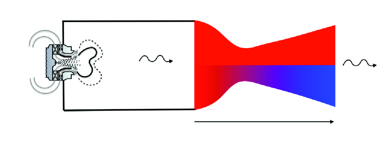
Reducing noise pollution around airports and heliports has become a significant concern due to stricter regulations and associated environmental challenges (European Environment Agency 2020). To address noise pollution, particularly from engines, efforts have primarily focused on reducing jet and fan noise. However, combustion noise has recently regained attention due to its increasing relative contribution to overall noise levels.
Combustion noise is split into two contributions. As flames are turbulent in the combustion chamber, this results in an unsteady combustion heat release, which leads to the generation of noise known as direct noise. Moreover, the exhaust gases downstream of the combustion chamber exhibit inhomogeneities in temperature and composition, along with the presence of vortical structures. As these inhomogeneities travel through and are accelerated or decelerated by the turbine, they produce the so-called indirect noise (Marble & Candel Reference Marble and Candel1977).
The first evaluation of the noise generation mechanisms was proposed by Marble & Candel (Reference Marble and Candel1977), who provided analytical predictions through nozzles. This analytical model has been subsequently extended to turbine flows by Cumpsty & Marble (Reference Cumpsty and Marble1977). Nonetheless, previous models were limited to predicting the transfer function for zero-frequency perturbations, while the transfer function change with perturbation frequencies (Stow & Dowling Reference Stow and Dowling2001; Goh & Morgans Reference Goh and Morgans2011). To overcome this limit and extend to all perturbation frequencies, an exact solution of the quasi-one-dimensional Euler equations, describing wave propagation through a nozzle, has finally been proposed by Duran & Moreau (Reference Duran and Moreau2013). To do so, several assumptions are still assumed for modelling noise propagation through a nozzle (Duran & Moreau Reference Duran and Moreau2013), or any medium (Poinsot & Veynante Reference Poinsot and Veynante2012). However, the hypotheses have been progressively examined in the literature, as discussed below.
(i) Negligible viscous forces is a classical assumption that has been investigated recently in the literature (De Domenico, Rolland & Hochgreb Reference De Domenico, Rolland and Hochgreb2019; Huet, Emmanuelli & Ducruix Reference Huet, Emmanuelli and Ducruix2021; Jain & Magri Reference Jain and Magri2022). Various modelling approaches have been developed, but they have resulted in the lack of clear consensus on its importance. (ii) Zero volume heat sources. The presence of heat fluxes at the walls has been analytically investigated by Yeddula et al. (Reference Yeddula, Guzmán-Iñigo and Morgans2022a
). By extending the exact solution (Duran & Moreau Reference Duran and Moreau2013) accounting for heat source terms, significant influence on noise transfer functions has been reported, especially at low frequencies. Moreover, thermal diffusion within flows is neglected under this assumption, which has been numerically verified by Huet (Reference Huet2017) through a nozzle guide vane. (iii) Non-reactive flows. This last assumption was assessed first by Jain, Giusti & Magri (Reference Jain, Giusti and Magri2023), modelling only weakly reacting flows. (iv) Isentropic flow variation is a result of (i) , (ii) and (iii). (v) Linear perturbations are commonly assumed, but their effectiveness may be diminished in flow downstream of the combustion chamber, where temperature fluctuations like hot spots exist. To this aim, Huet & Giauque (Reference Huet and Giauque2013) proposed a nonlinear model. (vi) Single-species gas flow is also commonly assumed. Its extension to multi-species flow was first proposed by Magri, O’Brien & Ihme (Reference Magri, O’Brien and Ihme2016) and Magri (Reference Magri2017), showing significant indirect composition noise contributions. However, Gentil et al. (Reference Gentil, Daviller, Moreau and Poinsot2024a
,Reference Gentil, Daviller, Moreau, Treleaven and Poinsot
b
) demonstrated that the use of a variable dependent wave decomposition vector in Magri et al. (Reference Magri, O’Brien and Ihme2016) leads the models (Magri et al. Reference Magri, O’Brien and Ihme2016; Magri Reference Magri2017) to completely overestimate indirect compositional noise. To circumvent this issue, a new composition noise model has been proposed by Gentil et al. (Reference Gentil, Daviller, Moreau and Poinsot2024a
,Reference Gentil, Daviller, Moreau, Treleaven and Poinsot
b
) and validated with unsteady numerical simulations. (vii) Quasi-one-dimensional flow is an assumption that allows neglect of the transverse mean-flow contributions. To overcome this assumption, a new model, in which constant transverse mean and fluctuating flow contributions are accounted for, has been developed by Duran & Morgans (Reference Duran and Morgans2015) with the assumption of thin annular nozzles. Moreover, quasi-one-dimensional flow often results in an overestimation of indirect entropy or composition planar noise transfer function moduli. A correction for entropy planar waves can be applied, as studied and proposed by Yeddula et al. (Reference Yeddula, Guzmán-Iñigo, Morgans and Yang2022c
). Finally, the flow is assumed to be a (viii) calorifically perfect gas mixture, i.e. the specific heat capacities for the different flow species at constant pressure are set to constants (
 $c_{p,k} =$
constant). Yet, this assumption may lead to significant errors in combustion noise prediction of real turbines since the temperature is quite variable within the successive rows of a turbine. To sidestep that limit, thermally perfect gas flow can be considered, such that the specific heat capacity of the
 $k$
th species is temperature dependent,
 $c_{p,k} = c_{p,k}(T)$
. Huet (Reference Huet2017) firstly examined that assumption by performing unsteady simulations of single-species flow with superimposed entropy incident waves. These results highlighted
 $10\,\,\%$
variations in indirect entropy noise modulus prediction between the two mixture assumptions. Despite that, the study remains limited to the considered and simulated choked flow nozzle and a single mechanism.
This paper aims at numerically and analytically examining the impact of the mixture hypothesis in the propagation of all three mechanisms: direct, indirect entropy and compositional noise as well as for two different nozzle flow configurations: subsonic or choked. Several objectives are pursued below, namely: to better understand the underlying mechanisms of noise generation, to derive analytical prediction models for both mixture assumptions and to generalise results from Huet (Reference Huet2017).
After deriving the quasi-one-dimensional linearised Euler equations, the noise prediction model is analysed in § 2. Two analytical solutions of the resulting system of equations, based on the assumption of low perturbation frequencies and on the Magnus expansion that is extensively described in Blanes et al. (Reference Blanes, Casas, Oteo and Ros2009), are then studied. Both models extend the prior model of Gentil et al. (Reference Gentil, Daviller, Moreau and Poinsot2024a
,Reference Gentil, Daviller, Moreau, Treleaven and Poinsot
b
) to a thermally perfect gas mixture and for low-frequency and all frequency perturbations, respectively. Three simulation test cases, similar to those in Gentil et al. (Reference Gentil, Daviller, Moreau and Poinsot2024a
,Reference Gentil, Daviller, Moreau, Treleaven and Poinsot
b
), are then numerically studied and described in § 3, assuming both mixture assumptions. These three nozzle flows have been simulated with different types of incident wave at various frequencies using the
 $AVBP$
solver (Schønfeld & Rudgyard Reference Schønfeld and Rudgyard1999). The post-processed transfer function moduli are then compared with the analytical predictions. Lastly, a parametric study is carried out in § 4 in order to evaluate the relative errors in the steady-state mean-flow values and noise transfer function moduli, between considering constant and variable heat capacities, for various choked flow nozzle configurations.
2. Combustion noise prediction model for thermally perfect gas mixture flows
To model the behaviour of the gas flow mixture entering the nozzle, it is assumed hereafter to be multi-species, adiabatic, chemically frozen, thermally perfect, at high Reynolds number, reversible and thus isentropic, quasi-one-dimensional flow. Therefore, the conservation equations (Bailly, Bogey & Candel Reference Bailly, Bogey and Candel2010) reduce to the quasi-one-dimensional Euler equations as follows:
 \begin{equation} \frac {\textrm {D} \rho }{\textrm {D} t}+\rho \frac {\partial u}{\partial x} = - \frac { \rho u}{A} \frac { \partial A}{ \partial x} ,\qquad \rho \frac {\textrm {D} u}{\textrm {D} t}+\frac { \partial p}{ \partial x}=0,\qquad \frac {\textrm {D} s}{\textrm {D} t}=0 ,\qquad \frac {\textrm {D} Y_{k}}{\textrm {D} t} =0, \end{equation}
where the substantial derivative is defined as
 $({\textrm {D}}/({\textrm {D}t})) = ({\partial }/({\partial t})) + u ({\partial }/({\partial x}))$
;
 $\rho$
,
 $u$
,
 $p$
and
 $T$
are the fluid density, the axial velocity, the static pressure and the static temperature respectively;
 $s$
is the specific entropy;
 $Y_k$
are the mass fractions of the
 $k$
th species respectively.
The set of equations (2.1) is closed using the perfect gas law equation
 \begin{equation} p = \rho \frac {\mathcal{R}_{u}}{W} T = \rho \,r\,T ,\end{equation}
where
 $\mathcal{R}_{u}$
is the universal gas constant and
 $W$
is the mean molar mass such that:
 $1/W=\sum _{k=1}^{N} Y_k/W_k$
;
 $W_k$
is the molar mass of the
 $k$
th species;
 $N$
is the total number of species;
 $r$
is the specific mixture gas constant
 $r = \sum _{k=1}^{N} r_k Y_k$
and
 $r_k$
is the specific gas constant of the
 $k$
th species.
In the assumptions of a multi-species and thermally perfect gas mixture, the specific heat capacities of the
 $k$
th species are temperature dependent
 $c_{p,k} = c_{p,k}(T)$
and are expressed hereafter as a polynomial of degree
 $N_l$
in temperature
 $T$
such that
 \begin{equation} c_{p,k} = \sum _{l = 0}^{N_l} a_{k,l} T^l ,\end{equation}
where
 $a_{k,l}$
are the polynomial coefficients of the
 $k$
th species and
 $l$
is the superscript corresponding to the power. Other thermodynamic variables such as the specific heat capacity, specific enthalpy and specific entropy of the mixture can be further derived, as detailed in Appendix A.
Assuming small dimensionless fluctuations denoted by
 $(\hat {\ })$
around a steady-state mean flow, the quasi-one-dimensional (quasi-1-D) Euler equations (2.1) are linearised, describing thus the propagation of the fluctuations. This is achieved by taking into account variables for multi-species flows as outlined below
 \begin{equation} \begin{aligned} \rho = \bar {\rho } ( 1 + \hat {\rho }),\quad p = \bar {p}(1+ \bar {\gamma } \hat {p}),\quad u = \bar{u}(1+\hat {u}),\quad Y_k = \bar {Y}_k+\hat {Y}_k \\ s = \bar {s} + \bar {c}_p \hat {s}, \quad s_k = \bar {s}_k + \overline {c}_{p,k} \hat {s}_k, \quad \gamma = \bar {\gamma }(1 + \hat {\gamma }), \quad r = \bar {r}(1 + \hat {r}) \\ \quad T = \overline {T}(1 + \hat {T}), \quad c_{p} = \overline {c}_p(1 + \hat {c}_{p}), \quad c_{p,k} = \overline {c}_{p,k}(1+\hat {c}_{p,k}) ,\end{aligned} \end{equation}
where
 $\gamma = c_p/c_v$
is the adiabatic index,
 $c_v$
is the mixture specific heat capacity at constant volume and (
 $s_k, h_k$
) are the specific entropy and enthalpy of the
 $k$
th species.
The mean steady-state flow is a solution of the quasi-1-D Euler equations (2.1) and is expressed as follows:
 \begin{equation} \cfrac {\partial \bar {\rho } \bar{u} A}{\partial x} = 0, \quad \bar {\rho } \bar{u} \frac {\partial \bar{u}}{\partial x} + \frac {\partial \bar {p}}{\partial x}= 0 , \quad \bar{u} \cfrac {\partial \bar {s} }{\partial x} = 0, \quad \bar{u} \cfrac {\partial \bar {Y}_k }{\partial x} = 0, \quad \cfrac { \partial \bar {c}_p }{\partial x } = \kappa \cfrac { \partial \bar {T}}{\partial x }, \end{equation}
where
 $\kappa$
is defined in equation (A7).
Similarly, as defined by Gentil et al. (Reference Gentil, Daviller, Moreau and Poinsot2024a
,Reference Gentil, Daviller, Moreau, Treleaven and Poinsot
b
), the entropy fluctuation and mixture fraction space fluctuation, denoted
 $\hat {s}_n$
and
 $\hat {Z}$
, respectively, can be introduced when linearising, as also proposed in Magri et al. (Reference Magri, O’Brien and Ihme2016), Magri (Reference Magri2017) and Gentil et al. (Reference Gentil, Daviller, Moreau, Treleaven and Poinsot2024b
), and are defined such that
 \begin{equation} \hat {s}_n = \cfrac {s_n^{\prime }}{\bar {c}_p} = \sum _{k=1}^N \frac {\overline { c_{p,k} }}{\overline {c_{p}}} \bar {Y_k} \hat {s_k} = \hat {T} + (1-\bar {\gamma }) \hat {p} , \quad \hat {Y}_k = \frac { \textrm {d} Y_k}{ \textrm {d} Z} \hat {Z} \quad \text{and} \quad \left [\frac {\partial }{\partial t} + \bar{u}\frac {\partial }{\partial x} \right ] \hat {Z} = 0 .\end{equation}
Introducing the dimensionless fluctuations in (2.4),
 $\hat {s}_n$
and
 $\hat {Z}$
in equation (2.6) into equations (2.1) and neglecting higher-order terms, leads us to write the quasi-one-dimensional linearised Euler Equations for non-reacting, multi-species and thermally perfect gas flow as below
 \begin{align} \left [\cfrac {\partial }{\partial t} + \bar{u} \cfrac {\partial }{\partial x}\right ]\left ( \hat {p} - \hat {s}_n \right ) + \bar{u} \cfrac {\partial \hat {u}}{\partial x} & = 0 ,\end{align}
 \begin{align}\left [\cfrac {\partial }{\partial t} + \bar{u} \cfrac {\partial }{\partial x}\right ]( \hat {u} ) + \cfrac {\bar {c}^2}{ \bar{u} }\cfrac {\partial \hat {p}}{\partial x} & = -\left ( 2\hat {u} - \Lambda \hat {Z} - \hat {s}_n + \left [ -(\bar {\gamma }-1) + (\bar {\gamma }-1)^2 \cfrac {\kappa \bar {T}}{\bar {c}_p} \right ] \hat {p} \right ) \cfrac { \textrm{d} \bar{u}}{ \textrm{d} x}, \end{align}
 \begin{align} \left [\cfrac {\partial }{\partial t} + \bar{u} \cfrac {\partial }{\partial x}\right ] \hat {s}_n & = - \left ( \bar {\gamma }-1\right ) \bar {M}^2 \left [ \left ( \Lambda - \chi \right ) \hat {Z} - \cfrac {\kappa \bar {T}}{\bar {c}_p} \hat {s}_n \right ] \cfrac { \textrm{d} \bar{u}}{ \textrm{d} x} ,\end{align}
 \begin{align} \left [\cfrac {\partial }{\partial t} + \bar{u} \cfrac {\partial }{\partial x}\right ] \hat {Z} & = 0 ,\end{align}
where
 $\bar {M} = \bar{u}/\bar {c}$
is the mean Mach number
 \begin{equation} \Lambda = \sum _{k=1}^N \frac {\bar {W} }{W_k} \frac {\textrm {d} Y_k}{ \textrm {d} Z} \quad \text{and} \quad \chi = \sum _{k=1}^N \frac {\bar {c}_{p,k}}{\bar {c}_p} \frac {\textrm {d} Y_k}{ \textrm {d} Z}. \end{equation}
Compared with the multi-species model of Gentil et al. (Reference Gentil, Daviller, Moreau and Poinsot2024a ,Reference Gentil, Daviller, Moreau, Treleaven and Poinsot b ), the linearised continuity equation (2.7a ) and species equations (2.7d ) are consistent, whether assuming calorifically or thermally perfect gas mixtures. Yet, additional terms appear in the linearised momentum equation (2.7b ) and energy equation (2.7c ).
When the mean velocity is constant (homogeneous flow) within the system of equations (2.7), i.e.
 $\textrm{d}\bar{u}/\textrm{d}x = 0$
, four decoupled equations called the characteristic equations are obtained for the multi-species flow and correspond to
 \begin{equation} w^{+} = \hat {p} + \bar {M}\hat {u}, \qquad w^{-}= \hat {p} - \bar {M}\hat {u}, \qquad w^{s}_h = \hat {s}_n , \qquad w^{z} = \hat {Z}. \end{equation}
In contrast, when the mean flow is non-homogeneous, i.e.
 $\textrm{d}\bar{u}/\textrm{d} x \ne 0$
, these four waves become coupled through the mean-flow gradient
 $\textrm{d}\bar {M}/\textrm{d}x$
, as detailed below by introducing them into the system of equations (2.7)
 \begin{align} \left [\cfrac {\partial }{\partial t} + (\bar{u} + \bar {c}) \cfrac {\partial }{\partial x} \right ]w^+ & = \left \{ \cfrac {\eta ^+ - \alpha ^- \zeta }{\bar {M}} w^+ + \cfrac {\alpha ^+\zeta - \eta ^+}{\bar {M}} w^- + \iota ^+ \zeta w^s_h + \Gamma ^- \zeta w^z \right \} \bar{u}\cfrac {\textrm{d} \bar {M}}{\textrm{d} x} ,\end{align}
 \begin{align} \left [\cfrac {\partial }{\partial t} + (\bar{u}- \bar {c}) \cfrac {\partial }{\partial x} \right ]w^- & = \left \{ \cfrac {\alpha ^-\zeta - \eta ^-}{\bar {M}} w^+ + \cfrac {\eta ^- - \alpha ^+\zeta }{\bar {M}} w^- - \iota ^- \zeta w^s_h - \Gamma ^+ \zeta w^z \right \}\bar{u}\cfrac {\textrm{d} \bar {M}}{\textrm{d} x}, \end{align}
 \begin{align} \left [\cfrac {\partial }{\partial t} + \bar{u} \cfrac {\partial }{\partial x} \right ] w^s_h & = \left \{ \zeta \cfrac {\iota ^+ - \iota ^-}{2} w^s_h + \zeta \cfrac {\Gamma ^+ - \Gamma ^-}{2} w^z \right \} \bar{u}\cfrac {\textrm{d}\bar {M}}{\textrm{d} x},\\[-8pt]\nonumber \end{align}
 \begin{align} \left [\cfrac {\partial }{\partial t} + \bar{u} \cfrac {\partial }{\partial x} \right ] w^z & = 0 ,\end{align}
where the coefficients
 $\zeta , \alpha ^{\pm }, \iota ^{\pm }$
and
 $\Gamma ^{\pm }$
are given by
 \begin{align} \zeta & = \left ( 1 + \cfrac {\bar {\gamma }-1}{2}\bar {M}^2 - \cfrac {(\bar {\gamma }-1)^2}{2\bar {c}_p}\bar {M}^2 \kappa \bar {T} \right )^{-1}, \quad \eta ^{\pm } = \cfrac {1}{2}\left ( 1 \pm \cfrac {1}{\bar {M}}\right ) ,\end{align}
 \begin{align} \alpha ^{\pm } & = 1 \pm \cfrac {\bar {\gamma }-1}{2} \bar {M} \mp \cfrac {(\bar {\gamma }-1)^2}{2\bar {c}_p} \bar {M}\kappa \bar {T}, \quad \iota ^{\pm } = 1 \pm (\bar {\gamma }-1)\bar {M}\cfrac { \kappa \bar {T}}{\bar {c}_p}, \end{align}
 \begin{align} \Gamma ^{\pm } & = \Lambda \pm (\Lambda -\chi )(\bar {\gamma }-1)\bar {M} .\end{align}
Consequently, the propagation of waves (i.e. fluctuations) through a non-reacting, multi-species, isentropic and thermally perfect gas mixture flow within a nozzle is characterised by equations (2.10). When comparing with the system of equations in Gentil et al. (Reference Gentil, Daviller, Moreau and Poinsot2024a
,Reference Gentil, Daviller, Moreau, Treleaven and Poinsot
b
), only the coefficients
 $\zeta$
,
 $\alpha ^{\pm }$
and
 $\iota ^{\pm }$
are extended with additional terms linked to
 $\kappa$
, i.e. to the temperature dependency of the species specific heat capacities at constant pressure. On the one hand, the system of equations (2.10) reduces to the system of equations found in Gentil et al. (Reference Gentil, Daviller, Moreau and Poinsot2024a
,Reference Gentil, Daviller, Moreau, Treleaven and Poinsot
b
) when
 $\kappa = 0$
. On the other hand, when
 $\kappa \ne 0$
, the system of equations features almost similar noise generation mechanisms to those found in Gentil et al. (Reference Gentil, Daviller, Moreau and Poinsot2024a
,Reference Gentil, Daviller, Moreau, Treleaven and Poinsot
b
), although with different transfer functions because of the changes in the coefficients
 $\zeta$
,
 $\alpha ^{\pm }$
and
 $\iota ^{\pm }$
. More surprisingly, a new inherent mechanism is found when
 $\kappa \ne 0$
and
 $\textrm {d} \bar {M} / \textrm {d} x \ne 0$
and concerns the entropy wave equation (2.10c
). Indeed, the entropy wave acts as either a source or a destructive term of entropy when propagating through the nozzle. This is allowed by the coupling term denoted by,
 $S_{c_p}$
, which is given by
 $S_{c_p} = (\zeta /2) ( \iota ^+ - \iota ^- ) \bar{u} (\textrm {d} M / \textrm {d} x)$
. In a more comprehensive way, when the Mach number gradient is positive
 $\textrm {d} \bar {M} / \textrm {d} x \gt 0$
, the coupling term is positive, and the entropy acts itself as an entropy source term when propagating through the accelerating flow. On the contrary, when
 $\textrm {d} \bar {M} / \textrm {d} x \lt 0$
, the coupling term is negative and the entropy acts as a destructive entropy term. To back up this argument, it should be recalled that the dimensionless entropy fluctuation is defined as
 $\hat {s}_n = s_n^{\prime }/\bar {c}_p$
. In the case of accelerating and isentropic flow, the temperature decreases according to the total temperature conservation. As a result, the mixture specific heat capacity at constant pressure decreases, leading to an increase in the dimensionless fluctuation
 $\hat {s}_n$
, which consequently generates a source term. Note that this demonstration is likewise applicable for showing how it acts as a destructive term. Last but not least, it can be emphasised that the change in this entropy-to-entropy coupling is intricately tied to the variations in static temperature. Consequently, a significant change in static temperature, such as across a nozzle or blade row, must occur to give rise to this entropy–entropy coupling.
Two solutions of that system of equations (2.10) are proposed hereafter in the present study, namely an analytical solution for low-frequency perturbations and an exact solution for all frequencies.
2.1. Low-frequency analytical solution
Similarly as initiated by Marble & Candel (Reference Marble and Candel1977), low-frequency perturbations allow us to assume the nozzle to be compact, so that fluctuations upstream and downstream of any nozzle can be simply related through jump conditions. Thus, temporal gradients are dropped from the system of equations (2.10) (as
 $f \xrightarrow {} 0$
), hence reducing the system of equations to the conservative equations of so-called invariants, denoted
 $I$
, such that
 \begin{equation} \bar{u} \cfrac {\partial I_A}{\partial x} = 0, \quad \bar{u} \cfrac {\partial I_B}{\partial x} = 0, \quad \bar{u} \cfrac {\partial I_C}{\partial x} = 0 \quad \text{and} \quad \bar{u} \cfrac {\partial I_D}{\partial x} = 0 ,\end{equation}
where the latter four invariants, denoted
 $[I_A, I_B, I_C, I_D]$
, are provided as below
 \begin{align}I_{A}& = \hat {u} + \hat {p} - \hat {s}_n , \quad I_B = \cfrac { 1 }{ \bar {h}_t } \left ( \bar {c}_p \bar {T}\left [ \hat {s}_n + \left ( \bar {\gamma }-1\right )\bar {p} \right ] + \left [ \sum _{k=1}^N \bar {h}_k \cfrac {\textrm{d}Y_k }{ \textrm{d}Z }\right ] \hat {Z} + \bar{u}^2 \hat {u} \right ) , \end{align}
 \begin{align} I_{C} & = \cfrac {1}{\bar {s}}\left ( \left [ \sum \limits _{k=1}^{N} \bar {\beta }_k \cfrac {\textrm{d} Y_k }{ \textrm{d} Z }\right ] \hat {Z} + \bar {c}_p \hat {s}_n \right ), \quad I_{D} = \hat {Z}, \end{align}
with
 \begin{equation} \bar {h}_k = \sum _{l=1}^{N_l} \cfrac {a_{k,l}}{l +1}\bar {T}^{l+1} \quad \text{and} \quad \bar {\beta }_k = a_{k,0}\log {\bar {T}} + \sum \limits _{l=1}^{N_l} \cfrac {a_{k,l}}{l} \bar {T}^l - r_k \log {\bar {p}} .\end{equation}
Using the waves defined in equations (2.9) and noting the wave decomposition basis
 $\textbf {W} = [w^+, w^-, w^s_h, w^z ]^t$
, the invariant vector, denoted
 $\textbf {I} = [I_{A}, I_B, I_{C}, I_{D} ]^t$
, can be reformulated in terms of waves as follows:
 \begin{equation} \textbf {I} = \mathcal{D} \textbf {W} \quad \text{and} \quad \mathcal{D} = \left [ \begin{array}{c c c c } \eta ^+ & \eta ^- & -1 & 0 \\[5pt] \cfrac {\bar {c}^2}{2 \bar {h}_t}(1 + \bar {M}) & \cfrac {\bar {c}^2}{2 \bar {h}_t}(1 - \bar {M}) & \cfrac {\bar {c}_p \bar {T}}{\bar {h}_t} & \sum _{k=1}^N \cfrac {\bar {h}_k}{\bar {h}_t} \cfrac { \textrm { d} Y_k } {\textrm { d} Z} \\[15pt] 0 & 0 & \cfrac {\bar {c}_p}{\bar {s}} & \cfrac {1}{\bar {s}} \sum _{k=1}^N \beta _k \cfrac { \textrm { d} Y_k }{\textrm { d} Z} \\[15pt] 0 & 0 & 0 & 1 \end{array} \right ], \end{equation}
where
 $\eta ^{\pm }$
are provided in equation (2.11).
Finally, equations (2.12) allow us to shape the jump conditions between the nozzle inlet and outlet locations, denoted
 $in$
and
 $out$
, respectively, given by
 \begin{equation} \textbf {I}_{in} = \textbf {I}_{out} \quad \xrightarrow []{} \quad \mathcal{D}_{in} \textbf {W}_{in} = \mathcal{D}_{out} \textbf {W}_{out} .\end{equation}
The resolution of equation (2.16) depends on the nozzle flow regime. In the case of subsonic flow, the second columns of matrices
 $D_{in}$
and
 $D_{out}$
need to be permuted and changed in sign in order to isolate ingoing from outgoing waves, before solving the system (2.16). In the case of a choked flow nozzle, the subsonic nozzle part is solved up to the throat position where the flow is choked, i.e.
 $M = 1$
. This last condition corresponds to a specific boundary condition, as extensively described by Marble & Candel (Reference Marble and Candel1977) such that
 $M^{\prime } = 0$
. For a thermally perfect gas mixture flow, the boundary condition reads as follows:
 \begin{equation} w^- = R_{+,\star }^- w^+ + R_{s,\star }^- w^s_h + R_{z,\star }^- w^z ,\end{equation}
where the subscript
 $\star$
corresponds to the choked throat position and the reflection coefficients
 $R_{+,\star }^-,R_{s,\star }^-$
and
 $R_{z,\star }^-$
are given by
 \begin{equation} \begin{aligned} R_{+,\star }^- = \cfrac {3 - \bar {\gamma } + \left ( \bar {\gamma }-1\right ) \bar {\psi } }{ \bar {\gamma } + 1 - \left ( \bar {\gamma }-1\right ) \bar {\psi } } , \qquad R_{s,\star }^- = \cfrac {2 \left ( \bar {\psi } - 1 \right ) }{\bar {\gamma } + 1 - \left ( \bar {\gamma }-1\right ) \bar {\psi } } ,\\ R_{z,\star }^- =- 2 \cfrac { \Lambda + \left (\bar {\gamma }-1\right )\left ( \Lambda - \chi \right ) }{\bar {\gamma } + 1 - \left ( \bar {\gamma }-1\right ) \bar {\psi } } \qquad \text{and} \qquad \bar {\psi } = \cfrac {\bar {\gamma }-1}{\bar {c}_p} \kappa \bar {T} .\end{aligned} \end{equation}
Note that it can be verified that the reflection coefficients in equation (2.18) converge to the ones in Gentil et al. (Reference Gentil, Daviller, Moreau, Treleaven and Poinsot2024b
), when assuming a calorifically perfect gas mixture, i.e.
 $\kappa = 0$
.
Then, the other nozzle part (i.e. from the throat section to the nozzle outlet) described by equation (2.16) is directly solved knowing the invariants and waves at the nozzle throat.
The latter solution is suitable for fast computation of the nozzle transfer functions with the assumption of low-frequency perturbations. Nonetheless, this limitation is important while perturbations may not be considered only at low frequency (Duran & Moreau Reference Duran and Moreau2013). To overcome this constraining assumption, an alternative solution can be calculated for all frequencies, as presented below.
2.2. Exact solution
An exact solution of the system of equations (2.10) is studied below, extending the prior work of Duran & Moreau (Reference Duran and Moreau2013) for a multi-species and thermally perfect gas mixture.
Introducing the dimensionless space and time variables
 $\xi = x/L_n$
and
 $\tau = tf$
, where
 $L_n$
is the nozzle length and
 $f$
is the perturbation frequency, the Helmholtz number
 $\Omega = f L_n/\bar {c}_{in}$
, where
 $\bar {c}_{in}$
is the inlet mean sound speed, and the reduced mean-flow velocity
 $\tilde {u}=\bar{u}/\bar {c}_{in}$
, the system of equations (2.7) can be rearranged as follows:
 \begin{align} \left [ \Omega \cfrac { \partial }{ \partial \tau } + \tilde {u} \cfrac { \partial }{ \partial \xi } \right ] I_{A} & = \tilde {u} \cfrac {\bar {s}\bar {T} }{ \bar{u}^2 } \cfrac {\partial I_{C} }{\partial \xi } - \cfrac {\tilde {u}}{ \bar{u}^2 } \left [ \sum \limits _{k=1}^{N} \left ( \bar {\beta }_k \bar {T} - \bar {h}_k \right ) \cfrac {\textrm {d} Y_k}{ \textrm {d} Z } \right ] \cfrac {\partial I_D }{\partial \xi } - \tilde {u} \cfrac {\bar {h}_t}{\bar{u}^2} \cfrac {\partial I_B }{\partial \xi } ,\end{align}
 \begin{align} \left [ \Omega \cfrac { \partial }{ \partial \tau } + \tilde {u} \cfrac { \partial }{ \partial \xi } \right ] I_B & = - \cfrac {\tilde {u} \bar {c}^2}{\bar {h}_t} \cfrac {\bar {s} }{\bar {c}_p} \cfrac {\partial I_{C} }{\partial \xi } + \cfrac {\tilde {u} \bar {c}^2}{\bar {h}_t} \cfrac { 1 }{\bar {c}_p} \left [\sum \limits _{k=1}^{N} \bar {\beta }_k \cfrac {\textrm {d} Y_k}{ \textrm {d} Z } \right ] \cfrac {\partial I_D }{\partial \xi } - \cfrac {\tilde {u} \bar {c}^2}{\bar {h}_t} \cfrac {\partial I_{A} }{\partial \xi } ,\end{align}
 \begin{align} \left [ \Omega \cfrac { \partial }{ \partial \tau } + \tilde {u} \cfrac { \partial }{ \partial \xi } \right ] I_{C} & = 0,\\[-10pt]\nonumber \end{align}
 \begin{align}\left [ \Omega \cfrac { \partial }{ \partial \tau } + \tilde {u} \cfrac { \partial }{ \partial \xi } \right ] I_D & = 0 .\end{align}
Assuming harmonic perturbations (
 $\textbf {I} = \textbf {I} e^{i\omega t}$
), the system (2.19) reads
 \begin{equation} \textbf {E}(\xi ) \cfrac {\textrm {d} \textbf {I}}{\textrm {d} \xi } = 2\pi \textrm {i} \Omega \textbf {I} ,\end{equation}
where
 $\textrm {i}$
is a pure imaginary complex and the matrix
 $\textbf {E}$
is given by
 \begin{equation} \textbf {E} = - \tilde {u} \left [ \begin{array}{cccc} 1 & \cfrac {\bar {h}_t}{\bar{u}^2 } & -\cfrac {\bar {s}\bar {T} }{ \bar{u}^2 } & \cfrac {1}{ \bar{u}^2 } \left [ \sum \limits _{k=1}^{N} \left ( \bar {\beta }_k \bar {T} - \bar {h}_k\right ) \cfrac {\textrm {d} Y_k}{ \textrm {d} Z } \right ] \\[15pt] \cfrac {\bar {c}^2 }{\bar {h}_t} & 1 & \cfrac {\bar {c}^2}{\bar {h}_t} \cfrac {\bar {s} }{\bar {c}_p} & -\cfrac {\bar {c}^2}{\bar {h}_t} \cfrac { 1 }{\bar {c}_p} \left [\sum \limits _{k=1}^{N} \bar {\beta }_k \cfrac {\textrm {d} Y_k}{ \textrm {d} Z } \right ] \\[15pt] 0 & 0 & 1 & 0 \\[5pt] 0 & 0 & 0 & 1 \end{array} \right ] .\end{equation}
When
 $\bar {M} \ne 1$
, the matrix
 $\textbf {E}$
is invertible and leads to
 \begin{equation} \cfrac {\textrm {d} \textbf {I}}{\textrm {d} \xi } = \mathcal{A}(\xi ) \textbf {I}, \end{equation}
where the matrix
 $\mathcal{A}$
is a non-constant matrix given by
 \begin{align} &\mathcal{A} = \cfrac {-2\pi i \Omega }{ \tilde {u} \left ( \bar {M}^2 - 1 \right ) } \nonumber\\&\left [ \!\!\begin{array}{cccc} \bar {M}^2 & - \cfrac {\bar {h}_t}{\bar {c}^2} & \cfrac {\bar {s}}{\bar {r}} & \cfrac { 1 }{\bar {c}^2} \left [ \sum \limits _{k=1}^{N} \left ( \bar {h}_k - \bar {\beta }_k \bar {\gamma } \bar {T} \right ) \cfrac {\textrm {d} Y_k}{ \textrm {d} Z } \right ] \\[15pt] - \cfrac {\bar{u}^2}{\bar {h}_t } & \bar {M}^2 & -\cfrac {\bar {s}\bar {T} }{ \bar {h}_t} \left ( 1 + \left ( \bar {\gamma }-1 \right ) \bar {M}^2 \right ) & \cfrac {1}{ \bar {h}_t } \left [ \sum \limits _{k=1}^{N} \left ( \bar {\beta }_k \bar {T} \left [ 1 + \left (\bar {\gamma }-1 \right ) \bar {M}^2\right ] - \bar {h}_k \right ) \cfrac {\textrm {d} Y_k}{ \textrm {d} Z } \right ] \\[15pt] 0 & 0 & \bar {M}^2 - 1 & 0 \\[5pt] 0 & 0 & 0 & \bar {M}^2 - 1 \end{array} \!\!\right ] .\end{align}
An exact solution for this system of equations (2.22) can be computed based on a Magnus expansion and depending on the nozzle flow regimes, as already extensively detailed in Duran & Moreau (Reference Duran and Moreau2013) and Gentil et al. (Reference Gentil, Daviller, Moreau, Treleaven and Poinsot2024b
). Finally, by using the subscripts
 $in$
and
 $out$
to describe variables at the nozzle inlet and outlet positions, respectively, the transfer functions are defined as follows:
 \begin{align} R_{aa} & = \cfrac {w^-_{in}}{w^+_{in}}, \quad T_{aa} = \cfrac {w^+_{out}}{w^+_{in}} ,\end{align}
 \begin{align} R_{ea} & = \cfrac {w^-_{in}}{w^s_{h,in}}, \quad T_{ea} = \cfrac {w^+_{out}}{w^s_{h,in}}, \quad T_{ee} = \cfrac {w^s_{h,out}}{w^s_{h,in}} ,\end{align}
 \begin{align} R_{ca} &= \cfrac {w^-_{in}}{w^z_{in}}, \quad T_{ca} = \cfrac {w^+_{out}}{w^z_{in}}, \quad T_{ce} = \cfrac {w^s_{h,out}}{w^z_{in}}, \quad T_{cc} = \cfrac {w^z_{out}}{w^z_{in}} ,\end{align}
where the subscripts of the coefficients
 $ea$
,
 $ee$
,
 $aa$
,
 $ca$
,
 $ce$
and
 $cc$
stand for the type of mechanism involved: the entropy-to-acoustic, entropy-to-entropy, acoustic-to-acoustic, composition-to-acoustic, composition-to-entropy and composition-to-composition mechanisms, respectively. These latter transfer functions are about to be evaluated in some specific test cases and referred to as ‘non-compact solution’.
3. Validation and results
To validate the analytical model for non-constant
 $c_p$
, unsteady simulations of an axisymmetric nozzle have been performed pulsing either incident acoustic, entropy or compositions waves, and using either calorifically or thermally perfect gas mixtures with the solver
 $AVBP$
(Schønfeld & Rudgyard Reference Schønfeld and Rudgyard1999). This explicit, high-order, unstructured and massively parallel solver is applied for solving the compressible Euler equations. Pulsing waves at various frequencies simultaneously allow us to evaluate the characteristic transfer function moduli of the nozzle across a range of frequencies, which can then be compared with the analytical predictions.
As initially investigated in the literature by Gentil et al. (Reference Gentil, Daviller, Moreau, Treleaven and Poinsot2024b ), the three nozzle configurations in the latter are studied again below, as they serve as reference test cases. Thus, these three test cases are firstly described in § 3.1.
After pulsing the different types of incident waves in each configuration, the waves are evaluated from the unsteady simulation results upstream and downstream of each nozzle, as described in Gentil et al. (Reference Gentil, Daviller, Moreau, Treleaven and Poinsot2024b ). Consequently, the transfer function moduli, defined in equations (2.24) are then accessed. Finally, a comparison in the modulus of the transfer function between the exact analytical prediction and the unsteady simulation results is studied.
3.1. Description of the three test cases
The first two test cases involve predicting transfer functions related to the propagation of inlet composition, entropy and acoustic waves through a nozzle, which is either choked or subsonic, and considering either constant or variable specific heat capacities. The latter geometry corresponds to the nozzle of Goh & Morgans (Reference Goh and Morgans2011), meshed using 17 419 triangular cells, and set up with the boundary conditions illustrated in figure 1, similarly to Gentil et al. (Reference Gentil, Daviller, Moreau, Treleaven and Poinsot2024b
). In both cases, each flow is initialised with the mean-flow solution, firstly computed from the mean-flow conditions summed up in table 1. It is noteworthy that the outlet static pressure is fixed to
 $p_{out} = 1.01325 \times 10^{5}$
Pa for the subsonic regime, whereas no outlet static pressure is imposed for the choked flow regime.
Description of the three test cases with the nozzle type, regime, inlet mean flow, mean species composition and considered species fluctuations.

Axisymmetric nozzle domain (x,y) with boundary conditions.

The Navier–Stokes characteristic boundary conditions, described in Gentil et al. (Reference Gentil, Daviller, Moreau, Treleaven and Poinsot2024b
), are used to handle the boundary conditions. Furthermore, composition, entropy and acoustic fluctuations are superimposed separately at the nozzle inlet and simultaneously at 20 different frequencies with a fundamental one at 200 Hz (
 $f \in [0.2, 4]$
kHz). Two points should be noted hereafter: the amplitudes of the considered species fluctuations, listed in table 1, are divided by the number of pulsed frequencies in order to avoid negative species mass fractions, and a constant and random phase shift is added to decorrelate the pulsed frequencies (Duran & Moreau Reference Duran and Moreau2013). Last but not least, the Euler equations are solved for the axisymmetric nozzle using the perfect gas equation (2.2), either constant or variable specific heat capacities and the Lax–Wendroff convection scheme. Finally, a Courant–Friedrichs–Lewy (CFL) number of
 $0.7$
is considered and a total simulation time of
 $T_{sim}=0.4 \textrm {s}$
is achieved for each case.
The final test case is designed to compare the outcomes of the exact analytical model discussed in § 2 assuming either constant or variable specific heat capacities in the unsteady simulation results. To proceed accordingly, the nozzle of Magri (Reference Magri2017), illustrated in figure 2 with the employed boundary conditions, is meshed using
 $21\,5200$
triangle cells as in Gentil et al. (Reference Gentil, Daviller, Moreau, Treleaven and Poinsot2024b
). The flow is then initialised with the mean-flow solution, firstly computed from the mean-flow conditions listed in table 1. Furthermore, no outlet static pressure is imposed downstream of the nozzle, since the nozzle flow regime is choked. Boundary conditions are handled and applied similarly as described for the two first test cases, except that the amplitudes of the species fluctuations are listed in table 1 and divided by the number of pulsed frequencies (20) to avoid negative species mass fractions. Lastly, the Euler equations are solved using the perfect gas equation (2.2), a two-step Taylor–Galerkin convection scheme, which is fourth-order accurate in time and third-order accurate in space (Colin & Rudgyard Reference Colin and Rudgyard2000), a CFL number of
 $0.7$
and a total simulation time of
 $T_{sim}=0.4$
s.
Nozzle computational domain and boundary conditions.

3.2. Steady-state mean flows
For each of the cases in table 1, the steady-state 1-D mean flow is solved analytically as described in Appendix B.1, and compared with the cross-sectionally averaged profiles of mean-flow values from
 $AVBP$
in figures 8, 9 and 10 provided in Appendix B.2. As a result, all mean-flow profiles post-processed from the simulations align closely with the analytical 1-D profiles, validating the assumption of quasi-1-D flow within the nozzles.
3.3. Case 1. Subsonic nozzle
The moduli of acoustic transfer functions are calculated analytically with the exact solution and compared with post-processed simulation results from
 $AVBP$
. The results are actually provided in figure 11 in Appendix B.3, since both the simulation and analytical results are close, alongside with the analytical predictions whatever the mixture assumptions. This result can be attributed to the minimal variation in static temperature along the nozzle (figure 8), leading to negligible changes in mixture heat capacity. As a result, there are only minor differences in the coefficient
 $\kappa$
and, consequently, in the coefficients
 $\zeta$
,
 $\alpha ^{\pm }$
and
 $\iota ^{\pm }$
(2.11). Finally, this leads to small differences, less than
 $5\,\%$
for convergent pulsed waves (i.e.
 $f\gt 0.5$
kHz), in the transmission transfer function modulus between both mixture assumptions.
3.4. Case 2. Choked nozzle
The moduli of transfer functions, listed and defined in equations (2.24), are provided in figure 3 for the choked nozzle of Goh & Morgans (Reference Goh and Morgans2011). While there are almost no differences in the reflection transfer function moduli whatever the type of incident wave, differences are mostly observed for transmission transfer function moduli involving the entropy wave:
 $|T_{ea}|$
,
 $|T_{ce}|$
and
 $|T_{ee}|$
. For the composition-to-entropy transfer function modulus
 $|T_{ce}|$
, analytical and numerical (
 $AVBP$
) results are consistent with each other, showing a maximum relative error of
 $\pm 1.2\,\%$
. In contrast, the results for
 $|T_{ea}|$
and
 $|T_{ee}|$
highlight more significant differences, reaching up to
 $\pm 5\,\%$
. Interestingly, the relative error in
 $|T_{ee}|$
between considering constant and variable specific heat capacities is constant whatever the perturbation frequencies. This outcome can be demonstrated theoretically, recalling the definition of
 $|T_{ee}|$
in equation (2.24b
). Indeed, a difference in transfer function modulus
 $|T_{ee}|$
is simply linked to the scaling of the entropy waves between the inlet outlet positions, namely
 $c_p(T_{in})$
and
 $c_p(T_{out})$
, respectively, such that
 $|T_{ee}|$
can be written as below
 \begin{equation} |T_{ee}| = \cfrac {w^s_{h,out}}{w^s_{h,in}} = \cfrac { s^{\prime }_{out}/c_p(T_{out}) }{ s^{\prime }_{in}/c_p(T_{in}) } = \cfrac { c_p(T_{in}) }{c_p(T_{out})} = 1.042 \quad \text{since $s^{\prime }_{in} = s^{\prime }_{out}$} .\end{equation}
On the contrary, the ratio of the transfer function modulus
 $|T_{ea}|$
predicted assuming a thermally and calorifically perfect gas mixture, evaluated in figure 12 and provided in Appendix B.4, highlights that the relative errors in
 $|T_{ea}|$
are not simply caused by the scaling of the entropy wave. Indeed, the previous ratio, close to
 $1.06$
, does not correspond to the ratio obtained for
 $|T_{ee}|$
, indicating that the origin of the gaps is also linked to the propagation operator. Overall, the frequency dependency of the reflection and transmission transfer function moduli computed with
 $AVBP$
corroborates the predicted ones using the exact solution described in § 2.2, extending the validation of the prediction model.
Modulus of the reflection and transmission transfer functions for various frequencies and test case 2. Non-compact:
 $c_p = cst$
(
 ),
 $c_p(T)$
(
 ).
 $AVBP$
:
 $c_p=cst$
(
 $\circ$
) and
 $c_p(T)$
(
 ).

Modulus of the reflection and transmission transfer functions for various frequencies and test case 3. Non-compact
 $c_p = cst$
(
),
 $c_p(T)$
(
).
 $AVBP$
 $c_p=cst$
(
 $\circ$
) and
 $c_p(T)$
(
).

3.5. Case 3. Choked nozzle
The moduli of the reflection and transmission transfer functions, computed analytically with the model in § 2 and numerically with
 $AVBP$
, are provided in figure 4 for the choked nozzle of Magri (Reference Magri2017) with the assumption of a calorifically and thermally perfect gas mixture. The reflection transfer functions moduli
 $|R_{aa}|$
,
 $|R_{ea}|$
and
 $|R_{ca}|$
are overall consistent with those predicted by the model considering either constant or variable specific heat capacities. Moreover, this hypothesis seems to have no significant impact on the reflection moduli. Similarly, the prediction of the acoustic-to-acoustic transmission transfer function modulus
 $|T_{aa}|$
by the model aligns closely with the numerical results, for all mixture assumptions. Conversely, differences appear for other transmission transfer functions, namely
 $|T_{ea}|$
,
 $|T_{ca}|$
,
 $|T_{ee}|$
,
 $|T_{ce}|$
,
 $|T_{cc}|$
where we notice an increasing gap with frequencies between the prediction and the corresponding simulation results. These frequency effects are well identified in the literature (Morgans, Goh & Dahan Reference Morgans, Goh and Dahan2013; Leyko et al. Reference Leyko, Duran, Moreau, Nicoud and Poinsot2014; Bauerheim et al. Reference Bauerheim, Duran, Livebardon, Wang, Moreau and Poinsot2016; Yeddula et al. Reference Yeddula, Guzmán-Iñigo, Morgans and Yang2022c
) and are caused by the propagation of waves
 $w^z$
and
 $w_{s,h}$
through non-uniform flows, i.e. at different convection speeds in the transverse direction. To support the latter, the profile of non-uniform axial velocity along the nozzle is provided in figure 13 in Appendix B.5. Aside from these frequency effects, it can be verified that the predictions of these transmission transfer function moduli using the analytical models converge with the simulation results at the zero-frequency perturbation for each mixture assumption.
Last but not least, differences in the transmission transfer function modulus between each mixture assumption are noteworthy for
 $|T_{ea}|$
,
 $|T_{ee}|$
and
 $|T_{ce}|$
, as for the other choked nozzle presented in § 3.4. These discrepancies begin even at low-frequency perturbations, with relative errors reaching just over 5 % for
 $|T_{ee}|$
, 1 % for
 $|T_{ce}|$
and under 7 % for
 $|T_{ea}|$
compared with the results assuming constant heat capacities.
To put in a nutshell, reflection transfer function moduli are almost not sensitive to the mixture assumption and to the nozzle flow regime: subsonic or choked. On the contrary, only some specific transmission transfer function moduli are altered by the mixture assumption when the flow is choked. In particular, the definition of the transmission moduli involving the entropy wave shows the greatest discrepancies between the two mixing hypotheses.
4. Parametric study and transfer function comparisons
A parametric study is proposed hereafter in order to evaluate the relative errors on the steady-state mean-flow values and on the noise transfer function moduli defined in equations (2.24), between considering constant and variable heat capacities, for various nozzle configurations. As concluded in § 3, the choked flow regime implies a greater temperature gradient and thus greater gaps in the transmission transfer function moduli. Therefore, only the choked flow regime is about to be considered in the following, in addition to being the most representative regime at take-off conditions. In the following, note that the notation has been dropped from the steady-state variables for the sake of clarity.
Prior to proceeding further, the choice of fixing the specific heat capacity constants (at constant pressure), determined at a certain static temperature, may modify significantly the mean-flow path and noise predictions. In contrast, this choice vanishes when directly considering thermally perfect gas mixtures. As an example from the literature and according to the kinetic theory of ideal gases, the air is commonly assumed to be a diatomic ideal gas such that
 \begin{equation} c_ p =\cfrac {7}{2} \cfrac {\mathcal{R}_u}{W}, \quad c_v = \cfrac {5}{2} \cfrac {\mathcal{R}_u}{W}, \quad \gamma = \cfrac {7}{5} = 1.4, \quad \text{where} \quad T = 300\ \text{K}. \end{equation}
Nonetheless, the specific heat capacities
 $c_p$
and
 $c_v$
are functions of temperature and a more suitable choice may be to fix them constant at the static temperature, computed at the nozzle inlet assuming variable specific heat capacities, denoted
 $T_{in}$
.
As such, three cases are investigated for a pure air stream with the following assuming: variable heat capacities termed ‘case ref.’ constant heat capacities fixed at
 $T_{in}$
termed ‘case 1’ and constant heat capacities fixed at
 $T = 300$
K termed ‘case 2’. Influence of the three mixture assumptions on the steady-state mean flow and on the transmission transfer function moduli for the lowest-frequency perturbations (analytical solution described in § 2.1) are evaluated in § 4.1. Finally, a multi-species gas mixture is also studied in order to assess the influence of the mixture assumptions on species transfer function moduli.
4.1. Pure air stream
The parametric study consists of varying the inlet and outlet Mach numbers,
 $M_{in} \in [0.1, 0.9]$
and
 $M_{out} \in [1.1, 2]$
, respectively, while the inlet total temperature is fixed
 $T_{t,in} = 1050$
K. The mean flow of all cases is solved as described in Appendix C.1. For cases 1 and 2, while relative errors in mean-flow values at the nozzle inlet shown in figure 14 in Appendix C.2 are less than 2 % , those at the outlet nozzle are compared with case ref. in figure 5 for various (
 $M_{in},M_{out}$
). The relative errors in the outlet steady-state mean flows reach up to
 $- 7 \ \,\%$
for
 $T_{out}$
and
 $p_{out}$
for case 2, while they remain below
 $\pm 2.6\ \,\%$
for case 1. Consequently, the choice of static temperature in fixing constant heat capacities significantly alters the steady-state mean-flow variables.
Relative errors in the steady-state outlet mean-flow values
 $[p_{out}, T_{out}, u_{out}, M_{out}]$
for case 1 (upper figures) and case 2 (bottom figures), compared with the case ref., and various (
 $M_{in},M_{out}$
).

After propagating the waves upon the mean flow for case ref., the modulus of the acoustic-to-acoustic, entropy-to-acoustic and entropy-to-entropy transmission transfer functions, denoted
 $|T_{aa}|_{Ref}$
,
 $|T_{ea}|_{Ref}$
and
 $|T_{ee}|_{Ref}$
, respectively, are presented in figure 6. Moreover, the relative errors for cases 1 and 2 are also compared with case ref. Figure 6 highlights discrepancies up to
 $5.5\,\%$
in
 $|T_{aa}|_{Ref}$
for case 2, whereas they are beneath
 $1\,\% |T_{aa}|_{Ref}$
for case 1. Furthermore, differences in
 $|T_{ea}|_{Ref}$
lie between
 $-2\,\%$
and
 $-8.9\,\%$
for both cases 1 and 2. Finally, the modulus of
 $|T_{ee}|$
is superior to
 $1$
for case ref., and results in relative errors with cases 1 and 2 up to a maximum of
 $-6.6\ \,\% |T_{ee}|_{Ref}$
.
On the one hand, the relative differences in transfer function modulus for case 2 are most likely explained by the similar order of relative errors in the steady-state mean flows. On the other hand, fixing constant heat capacities at the nozzle inlet static temperature is a fair compromise (case 1) in order to lower relative errors in the predictions of steady-state mean-flow values and the direct noise modulus. However, the prediction of the indirect entropy noise modulus and the entropy-to-entropy transmission transfer function modulus remains sensitive to whether thermally or calorifically perfect gas is assumed, with relative errors up to
 $-8.9 \ \,\%$
.
Furthermore, it is worth mentioning here that the mean static temperature varies in a range between
 $- 41\,\%$
and
 $-6 \,\%$
, as illustrated in figure 15 in Appendix C.2, leading to a maximum underestimate in indirect entropy noise of almost
 $9\,\%$
when assuming a calorifically perfect mixture (case 1). In general, greater temperature gradients can be found downstream of the combustion chamber, in particular between fresh air injected (
 $\approx 300$
K) through dilution holes and burnt gases in the combustion chamber (
 $\approx 1000$
K). These steeper gradients may exacerbate the shortcomings in the prediction of indirect combustion noise.
The effect of the mixture assumption on indirect composition noise is then addressed in the subsequent section.
Values of
 $|T_{aa}|_{Ref}$
,
 $|T_{ea}|_{Ref}$
and
 $|T_{ee}|_{Ref}$
for case ref., in addition to the relative errors in transfer function modulus for case 1 and case 2 in comparison with case ref. for various (
 $M_{in},M_{out}$
).

4.2. Multi-species flow
To compare nozzle composition transfer functions on a similar framework with constant and variable specific heat capacities and upon a multi-species flow, some incident composition mean-flow values and fluctuations are essential. To accomplish this, the species fluctuations and mean-flow values outlined in table 1 (test case number 3) are used in the subsequent analysis. Various geometries and choked flow nozzles are investigated, based on the methodology described in § 4.1 for the pure air stream. Nevertheless, only case ref. and case 1 are studied hereafter.
As for the pure air stream, the very small differences between the inlet and outlet mean-flow variables, illustrated in Appendix C.3 and reaching a maximum relative error of 2.7 %, can be considered negligible. After propagating waves through the choked nozzle in the compact assumption, the composition-to-acoustic
 $|T_{ca}|_{Ref}$
and composition-to-entropy
 $|T_{ce}|_{Ref}$
transmission transfer function moduli are presented in figure 7 for both cases. It is noteworthy that other moduli of the transmission transfer function are provided instead in Appendix C.4, since they do not provide any additional or different information than already commented for the pure air stream case. Almost no relative discrepancies in
 $|T_{ca}|_{Ref}$
are recovered for case 1, although they lie between
 $0\,\%$
and
 $-4\,\%$
of
 $|T_{ce}|_{Ref}$
. Consequently, the choice of constant specific heat capacities fixed at the nozzle inlet static temperature (case 1) proves to be an effective compromise for minimising the prediction in the composition-to-acoustic and composition-to-entropy transfer function moduli compared with case ref.
Values of
 $|T_{ca}|_{Ref}$
and
 $|T_{ce}|_{Ref}$
for case ref in addition to the relative errors for case 1 for various (
 $M_{in},M_{out}$
).

5. Conclusion
A new system of quasi-one-dimensional linearised Euler equations has been derived to describe the propagation of fluctuations through nozzles for thermally perfect gas and multi-species mixtures. The resulting model stresses a new entropy-to-entropy mechanism due to the variation of
 $c_p$
along the nozzle and scaling of the entropy wave, which does not appear when assuming constant heat capacities.
Two analytical solutions have been derived from the model, one of which is a solution for low-frequency perturbations, while the other one is an exact solution of the underlying equations. Unsteady simulations of axisymmetric nozzles with superimposed inlet acoustic, entropy and composition planar waves at various frequencies have been performed. Post-processing of the simulation results allows the validation of previous analytical solutions for two different nozzles and flow regimes: subsonic and choked.
Overall, reflection transfer function moduli are less sensitive to the mixture assumptions, whereas only some specific transmission transfer function moduli are altered by them, in particular the ones involving the entropy wave in their definitions. This supports the numerical results found by Huet (Reference Huet2017) for incident entropy wave and extends them for incident acoustic and composition fluctuations. Aside from the 2-D effects linked to flow dispersion on transfer function moduli, two other reasons explain the resulting discrepancies, namely: the scaling of the entropy wave, and the propagation operator. Additionally, variations in the transmission transfer function modulus remain limited and are closely linked to the sharpness of the static temperature gradient. This explains why the greatest differences occur for the two chocked flow nozzle cases, whereas they are negligible for the subsonic nozzle case.
To further investigate the influence of the mixture assumptions, a parametric study has been conducted to evaluate the variation in mean-flow variables and characteristic transfer function modulus, considering various nozzle configurations and choked flows. To do so, a pure air stream and a multi-species flow have been studied. Fixing specific heat capacities either at the static temperature of inlet nozzle or 300 K leads to at most
 $10\,\%$
error in mean flow, direct noise and entropy/composition noise, whereas using a thermally perfect gas eliminates these errors.
Last but not least, these variations in transmission transfer function modulus are closely tied to the steepness of the static temperature gradient. Therefore, in turbine stages where significant static temperature gradients occur, it can be expected that the prediction of combustion noise will be sensitive to the mixture assumptions made. Furthermore, blade cooling is another factor that strengthens temperature gradients, encountered in the high pressure turbine parts. As a consequence, the relative errors in combustion noise predictions by models assuming constant heat capacities may be further amplified, compared with models assuming variable heat capacities. Few perspectives of that work can be conducted: by studying that mixture assumptions with heat sources, as first initiated by Yeddula et al. (Reference Yeddula, Guzmán-Iñigo and Morgans2022b ) for a calorifically and single species perfect gas mixture, or by studying the influence of the mixture assumption on the noise transfer function in a real turbine stage configuration.
Funding
The CIRRUS project has received funding from the Clean Sky 2 Joint Undertaking under the European Union’s Horizon 2020 research and innovation program under grant agreement N
 $^\circ$
886554. This publication reflects only the author’s view and the JU is not responsible for any use that may be made of the information it contains. This work was performed using HPC resources from GENCI-TGCC (Grant 2023-A0132B10157).
Declaration of interests
The authors report no conflict of interest.
Appendix A. Thermodynamic functions for thermally perfect gas mixtures
A.1. Specific entropy and enthalpy of an ideal gas:
 $s_k$

Differentiating the specific entropy and enthalpy of a pure species, denoted
 $s_k(T,p)$
and
 $h_k(T)$
, yields
 \begin{equation} \textrm {d}s_k = \left (\cfrac {\partial s_k}{\partial T}\right )_p \textrm {d} T + \left (\cfrac {\partial s_k}{\partial p}\right )_T \textrm {d} p \quad \text{and} \quad \textrm {d}h_k = \left (\cfrac {\partial h_k}{\partial T}\right )_p \textrm {d} T. \end{equation}
Since a perfect gas is considered, the partial derivatives are provided in DeHoff (Reference DeHoff1993) as follows:
 \begin{equation} \left (\cfrac {\partial s_k}{\partial T}\right )_p = \cfrac {c_{p,k}}{T}, \quad \left (\cfrac {\partial s_k}{\partial p}\right )_T = -\cfrac {r_k}{p} \quad \text{and} \quad \left (\cfrac {\partial h_k}{\partial T}\right )_p = c_{p,k}. \end{equation}
With the assumption of a thermally perfect gas, the specific heat capacity is considered to be temperature dependent:
 $c_{p,k} = c_{p,k}(T)$
. To allow simple algebraic integration of equations (A1), the specific heat capacity is expressed as a polynomial of degree
 $N_l$
in temperature
 $T$
as provided in equation (2.3).
Integrating equations (A1) from a reference state (
 $T^{\circ },p^{\circ }$
) to a considered state, denoted (
 $T,p$
), gives
 \begin{align} s_k & = s_k^{\circ } + a_{k,0} \log \left ( T\right ) - r_k \log \left (p\right ) + \sum _{l=1}^{N_l} \cfrac {a_{k,l}}{l} T^l ,\end{align}
 \begin{align} h_k & = h_k^{\circ } + \sum _{l = 0}^{N_l} \cfrac {a_{k,l}}{l+1} T^{l+1}, \end{align}
where
 $s_k^{\circ } = -a_{k,0} \log ( T^{\circ } ) + r_k \log (p^{\circ } )$
and
 $h_k^{\circ } = \sum _{l = 0}^{N_l} [a_{k,l}/(l+1)] (T^{\circ })^{l+1}$
.
A.2. Specific entropy and enthalpy of a mixture of ideal gases:
$s$

When considering a mixture of ideal gases, the specific heat capacities of the mixture becomes
 \begin{equation} \left . \begin{array}{l l } c_{p,k} & = \sum\limits _{l=0}^{N_l} a_{k,l} T^l \\[9pt] c_p & = \sum\limits _{k=1}^N c_{p,k} Y_k \end{array} \right \} \xrightarrow {} c_p = \sum _{k=1}^N \left ( \sum _{l = 0}^{N_l} a_{k,l} T^l \right ) Y_k ,\end{equation}
where
 $c_{p,k}$
are the specific heat capacities of the pure species.
In addition, the specific entropy and enthalpy of the mixture are provided by
 \begin{equation} s = \sum _{k=1}^N \left [ s_k - r_k \ln {(X_k)}\right ] Y_k \quad \text{and} \quad h = \sum _{k=1}^N h_k Y_k, \end{equation}
which becomes, when introducing equations (A3a ) and (A3b ),
 \begin{align} s & = s^{\circ } + \left ( \sum _{k=1}^N a_{k,0} Y_k \right ) \log \left ( T \right ) - r \log \left (p\right ) + \sum _{k=1}^N\left [ \sum _{l=1}^{N_l} \cfrac {a_{k,l}}{l} T^l - r_k \ln {(X_k)} \right ] Y_k ,\end{align}
 \begin{align} h & = h^{\circ } + \sum _{k=1}^N \left [ \sum _{l = 0}^{N_l} \cfrac {a_{k,l}}{l+1} T^{l+1} \right ] Y_k ,\end{align}
where
 $s^{\circ } = \sum _{k=1}^N s^{\circ }_k Y_k$
,
 $h^{\circ } = \sum _{k=1}^N h^{\circ }_k Y_k$
and
 $r = \sum _{k=1}^N r_k Y_k$
.
A.3. Linearisation of equations
If considering steady-state mean-flow values, the specific heat capacity, denoted
 $\bar {c}_p$
in equation (A4), is no longer zero as it is for calorically perfect gas mixtures and is provided such that
 \begin{equation} \cfrac { \partial \bar {c}_p }{\partial x } = \kappa \cfrac { \partial \bar {T}}{\partial x } \quad \text{where} \quad \kappa = \sum _{k=1}^N \left ( \sum _{l = 1}^{N_l} l a_{k,l} \bar {T}^{l-1} \right ) \bar {Y}_k .\end{equation}
Linearising the mixture specific entropy
 $s$
provided in equation (A6a
), with fluctuations in equations (2.4), and introducing the result in equation (2.1), finally provides
 \begin{equation} \cfrac {\mathrm{D} }{\mathrm{D} t}[\hat {T} + (1-\bar {\gamma }) \hat {p}] + \left ( \bar {\gamma }-1\right ) \bar {M}^2 \left [ \sum _{k=1}^N \left ( \cfrac {r_k}{r} - \cfrac { \bar {c}_{p,k} }{\bar {c}_p}\right ) \hat {Y}_k - \cfrac {\kappa \bar {T}}{\bar {c}_p} [\hat {T} + (1-\bar {\gamma }) \hat {p}] \right ] \cfrac {\textrm{d} \bar{u}}{ \textrm{d} x} = 0 ,\end{equation}
where
 $\bar {M} = \bar{u}/\bar {c} = \bar{u}/\sqrt {(\bar {\gamma } \bar {r} \bar {T})}$
is the mean axial Mach number.
Cross-sectionally averaged Mach number (a), static pressure (b), static temperature (c) and mixture heat capacity (d) profiles for test case 1 with subsonic flow: 1-D model with constant (
) and non-constant
 $c_p$
(
) and
 $AVBP$
with constant (
 $\circ$
) and non-constant
 $c_p$
(
).

Cross-sectionally averaged Mach number (a), static pressure (b), static temperature (c) and mixture heat capacity (d) profiles for test case 2 with choked flow: 1-D model with constant (
) and non-constant
 $c_p$
(
) and
 $AVBP$
with constant (
 $\circ$
) and non-constant
 $c_p$
(
).

Cross-sectionally averaged Mach number (a), static pressure (b), static temperature (c) and mixture heat capacity (d) profiles for case 3 with choked flow: 1-D model with constant (
) and non-constant
 $c_p$
(
) and
 $AVBP$
with constant (
 $\circ$
) and non-constant
 $c_p$
(
).

Appendix B. Mean flow and additional results
B.1. Quasi-one-dimensional mean flow through nozzles
Assuming steady-state variables within the equations (2.1) allows us to retrieve four invariants that are conserved along the nozzle. Note that the bar over a variable
 $X$
(
 $\overline {X}$
) is dropped hereafter for the sake of clarity. They correspond to the mass-flow rate invariant
 $\dot {m}$
, the total enthalpy invariant
 $h_t$
, the entropy invariant and the species mass fraction invariants. In addition to using equations (A6b
) and (A6a
), they read
 \begin{align} \dot {m} & = \rho u_x A = cst ,\end{align}
 \begin{align} h_t &= h + u^2/2 = \sum _{k=1}^N \left [ \sum _{l = 0}^{N_l} \cfrac {a_{k,l}}{l+1} \left ( T^{l+1} - (T^{\circ })^{l+1}\right ) \right ] Y_k + \cfrac {u_x^2}{2}=cst ,\end{align}
 \begin{align} s &= \left ( \sum _{k=1}^N a_{k,0} Y_k \right ) \log \left ( \cfrac {T}{T^{\circ }}\right ) - r \log \left (\cfrac {p}{p^{\circ }}\right )\nonumber\\& \quad + \sum _{k=1}^N\left [ \sum _{l=1}^{N_l} \cfrac {a_{k,l}}{l} \left ( T^l - (T^{\circ })^l \right ) - r_k \ln {(X_k)} \right ] Y_k =cst .\end{align}
The resolution of that flow within a nozzle for thermally perfect gas mixture is almost similar to the one provided for calorifically perfect gas mixture in Duran Garcia-Rama (Reference Duran Garcia-Rama2013). Depending on the considered flow regimes, the steady-state mean flow is solved differently. To do so, it is common to impose the inlet temperature and inlet mass-flow rate, denoted
 $T_{in}$
and
 $\rho u_{in}$
, instead of inlet static variables, in addition to the outlet static pressure denoted
 $p_{out}$
. Then, depending on the minimum cross-section ratio within the nozzle and outlet static pressure, the nozzle flow regime can be determined, before solving the flow across the overall nozzle.
B.2. Mean-flow comparison
The cross-sectionally averaged profiles of static pressure, static temperature, mixture heat capacity and Mach number from
 $AVBP$
are compared with the 1-D solutions along the nozzle in figure 8 for case 1 in figure 9 for case 2 and finally in figure 10 for case 3.
B.3. Case 1. Subsonic nozzle
While the predictions of the entropy and composition-to-acoustic transfer function moduli (figure 11) are within close range of the corresponding simulations results, the ones for incident acoustic waves have difficulty converging for the lowest-frequency perturbations. Nonetheless, the acoustic-to-acoustic transfer function moduli from the simulation are close, alongside the analytical predictions. Note that assuming constant or variable heat capacities does not significantly alter the transfer function moduli for the subsonic case.
Modulus of the reflection and transmission transfer functions for various frequencies. Non-compact:
 $c_p = cst$
(
),
 $c_p(T)$
(
) and
 $AVBP$
:
 $c_p=cst$
(
 $\circ$
) and
 $c_p(T)$
(
).

B.4. Case 2. Choked nozzle
For the choked flow nozzle of case 2, the ratio of the transfer function modulus
 $|T_{ea}|$
predicted assuming a thermally and calorifically perfect gas mixture is illustrated in figure 12.
Ratio of
 $|T_{ea}|_{c_p(T)} / |T_{ea}|_{c_p(T_{in})}$
predicted with analytical model (
) and computed with
 $AVBP$
for various frequencies (
 $\circ$
) for case 2.

B.5. Case 3. Choked nozzle
The steady-state field of axial velocity within the nozzle is illustrated in figure 13.
Contour of axial velocity in the choked nozzle of case 3.

Relative errors in the steady-state mean-flow values
 $[p_{in}, T_{in}, u_{in}, M_{in}]$
for case 1 (
 ) and case 2 (
 ), compared with case ref., and various
 $M_{in}$
.

Axial variation of static pressure (a), static temperature (b) and specific mixture heat capacity (c) along the nozzle for case ref.

Appendix C. Additional results for the parametric study
C.1. Mean-flow calculation
To impose a choked flow, it is common to impose the inlet isentropic total temperature and inlet total pressure, denoted
 $T_{t,in}$
and
 $p_{t,in}$
, instead of inlet static variables, in addition to the outlet static pressure, denoted
 $p_{out}$
. The parametric study to determine the mean flows and transfer functions is split hereafter over two regions: the subsonic region until the throat position, where
 $M_{\star } = 1$
, and the supersonic region until the nozzle outlet.
First region. The goal is to first consider case 1 with constant heat capacities. The evaluation of
 $T_{in}$
uses the definition of isentropic total temperature
 $T_{t,in}$
, considering different inlet Mach numbers, denoted
 $M_{in}$
. Then, the cross-section ratio between the inlet and throat sections, denoted
 $A_{in}/A_{\star }$
, is secondly determined, considering
 $M_{in}$
,
 $M_{\star } = 1$
and the constant heat capacities. Finally, imposing
 $T_{t,in}$
,
 $p_{t,in}$
, the steady-state mean-flow characteristics are then totally deduced at the nozzle inlet.
For the other mixture assumptions, similar cross-section
 $A_{in}/A_{\star }$
, total temperature
 $T_{t,in}$
, total pressure
 $p_{t,in}$
and throat Mach number
 $M_{\star } = 1$
are considered. Equations B1 are then solved for each mixture assumptions, resulting in the evaluation of
 $ [p_{in}, T_{in}, u_{in}, p_{\star }, T_{\star } ]$
.
Second region. For the second region, case 1 with constant heat capacities, fixed at
 $T_{in}$
, is first considered. Choosing different outlet Mach numbers, denoted
 $M_{out}$
, allows us to fix indirectly the cross-section ratio between the throat and outlet sections, denoted
 $A_{\star }/A_{out}$
, knowing
 $M_{throat}$
. After fixing the divergent nozzle geometry and since all flow variables are known at the throat position, the steady-state mean-flow characteristics at the nozzle outlet are then evaluated using equations (B1).
For the other mixture assumptions, similar cross-section ratios
 $A_{\star }/A_{out}$
are considered and since the mean-flow values are known at the throat position, all the outlet variables can be deduced, yielding:
 $ [p_{out}, T_{out}, u_{out} ]$
.
Relative errors in the steady-state inlet mean-flow values
 $[p_{in}, T_{in}, u_{in}, M_{in}]$
for case 1 compared with case ref. for various
 $M_{in}$
.

Relative errors in the steady-state outlet mean-flow values
 $[p_{out}, T_{out}, u_{out}, M_{out}]$
for case 1 compared with case ref. for various (
 $M_{in},M_{out}$
).

Axial variation of static pressure (a), static temperature (b) and specific mixture heat capacity (c) along the nozzle for case ref.

C.2. Pure air stream
The relative errors in the mean-flow values at the inlet nozzle are illustrated in figure 14, and compared with case ref. for various (
 $M_{in},M_{out}$
).
Values of
 $|T_{aa}|_{Ref}$
,
 $|T_{ea}|_{Ref}$
and
 $|T_{ee}|_{Ref}$
for case ref. in addition to the relative errors for case 1.

The axial variations in static temperature, static pressure and mixture heat capacity between the inlet and outlet nozzle positions are provided in figure 15 for case ref.
C.3. Multi-species flow
After solving for the mean-flow values for the multi-species flow, the relative errors in the inlet and outlet mean-flow variables are illustrated in figures 16 and 17, respectively, for case 1, and compared with case ref. for various (
 $M_{in},M_{out}$
).
C.4. Transmission transfer functions in the case of the multi-species mixture
The modulus of the acoustic-to-acoustic, entropy-to-acoustic and entropy-to-entropy transmission transfer functions for the multi-species mixture in § 4.2 and several choked flows are provided in figure 19. Overall, similar differences and orders of magnitudes are found with the case of pure air (§ 4.1) in terms of moduli of the transmission transfer functions
 $|T_{aa}|_{Ref}$
,
 $|T_{ea}|_{Ref}$
and
 $|T_{ee}|_{Ref}$
.



