1 Introduction
Ice sheets, such as those that cover Greenland and Antarctica, transport inland ice to the ocean. The flow of ice is driven by hydrostatic pressure gradients associated with the thickness and topography of the ice and resisted by viscous coupling at the base (Rignot, Mouginot & Scheuchl Reference Rignot, Mouginot and Scheuchl2011; Schoof & Hewitt Reference Schoof and Hewitt2013). While the topography and thickness of these land-fast ice masses have been carefully mapped using remote observations, it is more difficult to determine the spatial and dynamical pattern of coupling at the base. Previous efforts to constrain the basal conditions have included bore-hole measurements of subsurface conditions (Fischer et al. Reference Fischer, Iverson, Hanson, Hooke and Jansson1998; Clarke Reference Clarke2005), which provide pointwise estimates of basal properties, and large-scale inversions (Larour et al. Reference Larour, Seroussi, Morlighem and Rignot2012; Sergienko & Hindmarsh Reference Sergienko and Hindmarsh2013; Sergienko, Creyts & Hindmarsh Reference Sergienko, Creyts and Hindmarsh2014), which use the large-scale viscous flow of an ice sheet with known topography and surface velocity to infer the basal traction. Despite these efforts, the response to changing properties at the base of ice sheets remains poorly understood, particularly as the base of glaciers remains difficult to access. It has been observed that, in general, the flow of the Greenland ice sheet accelerates at the beginning of the melt season when much of the water is thought to be directed to the bed (Stevens et al. Reference Stevens, Behn, Das, I., Noel, van den Broeke and Herring2016), but questions remain as to the surface and subsurface hydrology of melt water and the spatial and temporal patterns of ice flow associated with enhanced melt rates. A contributing factor in the ambiguity between melt water production and basal sliding is the difficulty in quantifying the volume of melt water reaching the bed as a function of time. For this reason, observations of the response of glacial sliding to the drainage of a known volume of melt water from supraglacial lakes provide an important constraint on processes within the subglacial environment.
In the past decade, observations of the drainage of supraglacial lakes have been made in a number of melt seasons (Das et al.
Reference Das, Joughin, Behn, Howat, King, Lizarralde and Bhatia2008; Stevens et al.
Reference Stevens, Behn, McGuire, Das, Joughin, Herring, Shean and King2015), which help to constrain the local response to lake drainage events. Using seismometers, a surface GPS network and pressure transducers deployed within the supraglacial lakes, these studies characterised the precursor, drainage and sliding response of the ice sheet. Supraglacial lake drainage events can be extremely rapid, with large (
 $5{-}10~\text{km}^{2}$
) lakes draining in as little as 1–2 h. While there is some debate as to the mechanism by which these drainage events are initiated, the more recent observations suggest that catastrophic drainage is preceded by a slow uplift and increase in sliding velocity. This precursor, and its influence on the ice velocity, has been thought to indicate that some melt water initially lubricates the glacial bed, promoting divergence of the ice velocity field and fracturing. After this initial transient, observations suggest a measurable uplift of the ice in a broad, shallow dome, and a related patch of enhanced ice velocity, both of which spread with time (Stevens et al.
Reference Stevens, Behn, McGuire, Das, Joughin, Herring, Shean and King2015).
These observations of subglacial drainage have spurred a number of modelling studies, which have focused, in the main, on the initial hours of lake drainage. Tsai & Rice (Reference Tsai and Rice2010) used a two-dimensional theory of linear elastic fracture mechanics to model the growth of a subglacial cavity in which melt water fractures the contact between solid bedrock and elastic ice. Their study focused on the rapid drainage of the lake, attempting to quantify the rate of lake drainage by solving for the elastic deformation using a turbulent parameterisation for the flow of the subglacial water and a fracture criteria at the leading edge. Dow et al. (Reference Dow, Kulessa, Rutt, Tsai, Pimentel, Doyle, van As, Lindback, Pettersson, Jones and Hubbard2015) subsequently examined the formation of channelised flow in the larger-scale subglacial system around the drainage event, by coupling a model of turbulent, flow-driven fracture propagation (Tsai & Rice Reference Tsai and Rice2010) with a model of subglacial channel formation (Pimentel & Flowers Reference Pimentel and Flowers2011). Perhaps the most comparable study to the present investigation is that of Adhikari & Tsai (Reference Adhikari and Tsai2015), who examined the effect of a pre-existing drainage network. They modelled this network as a thin, pre-existing aperture below the ice, which acts as a pre-wetting film for the flow, by analogy with the study of laminar injection below an elastic sheet by Lister, Peng & Neufeld (Reference Lister, Peng and Neufeld2013). They again consider a planar cavity spreading below a semi-infinite elastic medium, and above a non-porous base, and apply a turbulent parameterisation of the flow throughout the fracture and the pre-existing hydrological network.
In this paper, we consider the impact of subglacial till, as modelled by a saturated, deformable porous layer, on the drainage of supraglacial lakes. More specifically, we develop a theoretical model accounting for the radial spread of fluid at the base of an elastic sheet resting on a saturated porous layer. The model describes the formation and spread of a subglacial, water-filled cavity driven by a rapid influx of lake water, providing localised flotation of the glacier, and the diffusion of pore pressure within, and leakage of fluid into, the subglacial till. We make a number of simplifying assumptions in order to focus on the fluid dynamical processes associated with spreading over a deformable porous base: we employ lubrication theory throughout, and assume an axisymmetric geometry, a simple rheological specification of the till and a simplified description of the flexural response of glacial ice as that of an elastic bending beam.
Beyond the direct application to supraglacial drainage, there has been renewed interest in the fluid mechanics associated with spreading below an elastic sheet, driven by applications in different settings including hydraulic fracturing (Wang & Detournay Reference Wang and Detournay2018), magmatic intrusions (Thorey & Michaut Reference Thorey and Michaut2016), soft robotics (Rubin et al. Reference Rubin, Tulchinsky, Gat and Bercovici2017) and control of viscous-fingering instabilities (Pihler-Puzovic, Juel & Heil Reference Pihler-Puzovic, Juel and Heil2014). It is well known that the spread of a shallow fluid layer beneath a bending elastic beam depends sensitively on the conditions at its front or nose (Lister et al. Reference Lister, Peng and Neufeld2013; Hewitt, Balmforth & De Bruyn Reference Hewitt, Balmforth and De Bruyn2015b ; Peng et al. Reference Peng, Pihler-Puzovic, Juel and Heil2015). In particular, within the framework of lubrication theory, fluid cannot propagate between an elastic sheet and the base without some form of regularisation at the nose, such as being connected to a thin pre-wetted fluid layer or the presence of a vapour tip near the nose. One of the primary goals of this work is to demonstrate that an underlying rigid or deformable porous layer allows propagation without any regularisation at the nose, and to explore the effects of such a layer on the dynamics of spreading.
We begin in § 2 with a description of the model set-up. In § 3 we consider laminar flow in the limit in which deformation of the till is negligible, and then re-introduce till deformation and diffusion of pore pressure in § 4. In § 5, we relax the assumption of laminar flow and, using a simple hybrid parameterisation, examine the role of turbulence on the spread of the subglacial cavity. Given the potential application of this work for enhanced understanding of the transient response of ice sheets to supraglacial lake drainage, we briefly discuss the relevance of our findings to recently published observations of lake drainage events in § 6.
2 Model set-up
Consider a glacier of thickness
 $d$
and density
 $\unicode[STIX]{x1D70C}_{i}$
resting on a shallow, deformable, porous and saturated till of unstressed thickness
 $b_{0}$
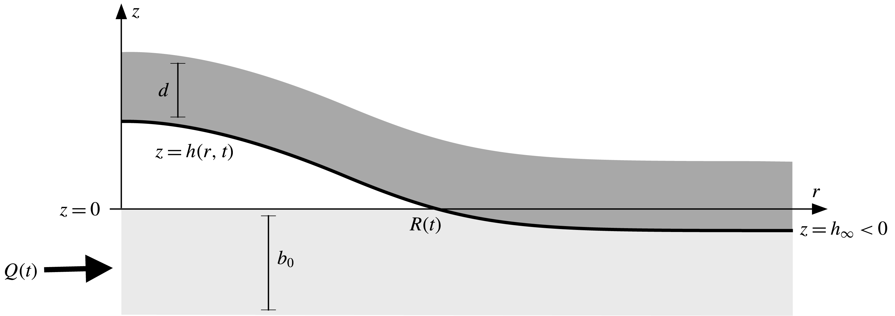
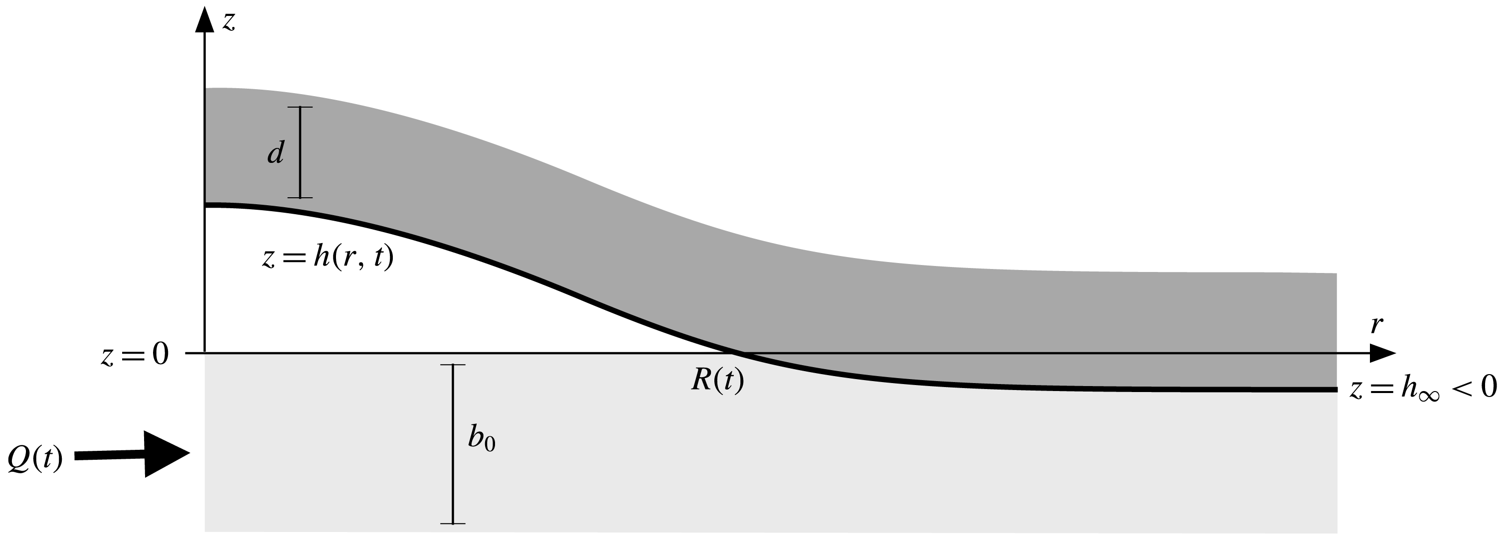
. Adhesive forces between the till and glacier are assumed to be weak, such that the glacier rests on the till rather than being frozen onto it, as would be the case for temperate glaciers or at the margins of the Greenland ice sheet during the melt season. For simplicity, in this derivation any basal topography is ignored, although it could readily be incorporated in the existing model framework. Motivated by the observations by Stevens et al. (Reference Stevens, Behn, McGuire, Das, Joughin, Herring, Shean and King2015) of a roughly radial signal, we assume the subglacial spreading is axisymmetric and work in a polar coordinate system
 $(r,z)$
, as sketched in figure 1, with the base height
 $z=0$
set to be level with the height of the unstressed till. At equilibrium, the till is compressed by the glacier below this point, such that the base of the glacier lies at a height
 $z=h_{\infty }\leqslant 0$
. Fluid is injected into the till beneath the glacier at
 $r=0$
with flux
 $Q(t)$
, causing the till to expand and the base of the glacier to rise to a height
 $z=h(r,t)$
. If sufficient fluid is injected, the till can expand to its unstressed height
 $h=0$
, and any increase in pressure beyond this point will cause the ice to lift off the till completely (
 $h>0$
), forming a fluid-filled cavity between the till and the ice (figure 1). If
 $h>0$
anywhere, we define the touchdown point or nose
 $r=R(t)$
of the cavity to be the smallest radius at which
 $h=0$
. Note that
 $Q(t)$
is simply a parameter in this model: we do not attempt to incorporate any description of how fluid propagates through the ice to its base (see e.g. Rice et al.
Reference Rice, Tsai, Fernandes and Platt2015).
Schematic (not to scale) of the rapid inflation of a subglacial cavity in a radial geometry, driven by an injection flux
 $Q(t)$
at the origin. The base of the glacier, which initially compresses the saturated till by an amount
 $-h_{\infty }$
, is uplifted to
 $z=h(r,t)$
. Where
 $h>0$
, a cavity of fluid opens up between the glacier and the fully expanded till, which has depth
 $b_{0}$
.
We proceed by assuming that the characteristic radial length scales of flow below the glacier are much larger than the uplift or the depth of the till, and so we use lubrication theory to describe the spreading through the till and cavity.
2.1 The till
We treat the till as a saturated, linear poroelastic medium, characterised by an effective stress tensor which is linearly related to the strain in the till. In the limit of a rigid till, the till reduces to a standard incompressible porous medium. In the shallow limit, we need only consider the vertical force balance on the till, which is dominated by the vertical normal stress
 $\unicode[STIX]{x1D6F4}$
(see e.g. Hewitt, Neufeld & Balmforth Reference Hewitt, Neufeld and Balmforth2015a
). The stress
 $\unicode[STIX]{x1D6F4}$
can be decomposed into the isotropic fluid pore pressure
 $p$
and an ‘effective’ network stress
 $\unicode[STIX]{x1D70E}$
, giving
 $\unicode[STIX]{x1D6F4}=p+\unicode[STIX]{x1D70E}$
(cf. Terzaghi’s principle in solid mechanics (Wang Reference Wang2000)). Given that deformations are small, the network stress
 $\unicode[STIX]{x1D70E}$
can be linearly related to the vertical strain
 $\unicode[STIX]{x1D716}$
via
 $$\begin{eqnarray}\unicode[STIX]{x1D70E}=-M\unicode[STIX]{x1D716},\end{eqnarray}$$
where
 $M=K+4G/3\gg 1$
is the stiffness (or, more precisely, the
 $p$
-wave modulus, defined in terms of the bulk and shear moduli of the till
 $K$
and
 $G$
; see Hewitt et al. (Reference Hewitt, Neufeld and Balmforth2015a
)).
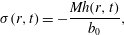
In steady state, the strain will, in general, vary through the depth of the till to balance the lithostatic gradient. If, however, the stiffness of the till is large (relative to its weight) then the variation in strain across the shallow till is small; equivalently, the compaction length of the till is much greater than its depth. In this limit, which we assume here, the strain is independent of depth to leading order, and the stress is thus
 $$\begin{eqnarray}\unicode[STIX]{x1D70E}(r,t)=-\frac{Mh(r,t)}{b_{0}},\end{eqnarray}$$
provided
 $h<0$
(such that there is no overlying cavity), and
 $\unicode[STIX]{x1D70E}=0$
otherwise. Strictly, equation (2.2) is a quasi-steady expression, which relies on an assumption that the till evolves rapidly in the vertical in response to a change in stress. This assumption is consistent with the shallow framework introduced in § 2.3. We note, however, that it could be violated if the external time scales of flow (at the injection point or nose of the cavity, for example) are much faster, as could be the case if the till permeability or stiffness is small (see § 2.5).
At equilibrium the till is compressed by the weight of the glacier alone. As such, the equilibrium height, or far-field compression height, is simply
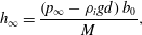 $$\begin{eqnarray}h_{\infty }=\frac{\left(p_{\infty }-\unicode[STIX]{x1D70C}_{i}gd\right)b_{0}}{M},\end{eqnarray}$$
where
 $p_{\infty }<\unicode[STIX]{x1D70C}_{i}gd$
is the background pore pressure in the till relative to atmospheric pressure. In the limit of a rigid porous till,
 $M\rightarrow \infty$
, the medium is able to withstand arbitrary stress, and so
 $h_{\infty }\rightarrow 0$
.
2.2 The ice
We work under the assumption that the uplift of the cavity and the depth of the till are small relative to the ice thickness
 $d$
, such that tensional stresses are negligible, and that the radial scales of the flow
 ${\sim}R(t)$
are long relative to
 $d$
. As such, we model the overlying ice as an elastic beam of bending stiffness
 $B=E_{i}d^{3}/12(1-\unicode[STIX]{x1D708}^{2})$
, in terms of its Young’s modulus
 $E_{i}$
and Poisson ratio
 $\unicode[STIX]{x1D708}$
. Ice uplifted by an amount
 $h(r)$
thus exerts a bending stress
 $B\unicode[STIX]{x1D6FB}^{4}h$
, where in radial coordinates
 $\unicode[STIX]{x1D6FB}^{4}=[r^{-1}\unicode[STIX]{x2202}_{r}(r\unicode[STIX]{x2202}_{r})]^{2}$
. This formulation transforms an otherwise non-local description of elastic deformation into a local bending-beam description, allowing for analytically tractable and interpretable solutions.
While the first assumption above is certainly reasonable, the second (
 $R\gg d$
) is less likely to be strictly valid in the geophysical context of subglacial drainage. The observations of Stevens et al. (Reference Stevens, Behn, McGuire, Das, Joughin, Herring, Shean and King2015) and the typical parameter ranges outlined in § 2.5 suggest that
 $R$
and
 $d$
are broadly comparable in size, although the radial scales of deformation in the till can be rather larger, while the region near the nose of the cavity, which is found below to play a crucial role in the dynamics, can be rather smaller. For the purposes of this paper, we nevertheless proceed under the assumption of a bending beam, in order to focus in detail on the effect of a porous and deformable substrate on the dynamics of a spreading cavity. Detailed study of the accuracy of the beam assumption in this context is left for future work, although we note that this issue was considered in a related study of turbulent fracture near a free surface (Tsai & Rice Reference Tsai and Rice2012).
Lastly, we also note that the ice in this model is purely elastic, and does not creep. This is likely to be a reasonable approximation over the relatively short time scales associated with the initial spread of the cavity (
 ${<}O(1)$
day), but we would expect viscous deformation to affect the forcing from, and response of, the ice at larger times.
2.3 Shallow-layer model
The shallow geometry indicates that vertical velocities are small, and hence that the fluid pressure
 $p$
in both the cavity and the till is hydrostatic,
 $$\begin{eqnarray}p(r,z,t)=P_{g}(r,t)+\unicode[STIX]{x1D70C}g(h-z),\end{eqnarray}$$
where
 $\unicode[STIX]{x1D70C}$
is the density of water and
 $P_{g}$
the pressure at the base of the ice. Above the fluid-filled cavity,
 $P_{g}$
simply consists of the overburden weight and the bending stresses of the ice. Where there is no cavity, however, part of the pressure from the ice is instead taken up by the network stress of the till itself, (equation (2.2)). Thus
 $$\begin{eqnarray}P_{g}(r,t)={\mathcal{H}}(-h)\frac{Mh}{b_{0}}+\unicode[STIX]{x1D70C}_{i}gd+B\unicode[STIX]{x1D6FB}^{4}h,\end{eqnarray}$$
where
 ${\mathcal{H}}$
is the unit Heaviside step function. The three terms in (2.5) represent, respectively, the network stress in the till, which is non-zero only when
 $h$
is negative, the weight of the overlying ice and the bending stresses from the overlying ice with bending stiffness
 $B$
.
The radial flow
 $u$
is given by Darcy’s law within the till. In the cavity, we initially assume that the flow remains laminar (we relax this assumption in § 5) and, as such, is described by standard lubrication theory with no slip beneath the glacier at
 $z=h$
. In both till and cavity, the flow is driven by the radial pressure gradient,
 $$\begin{eqnarray}\displaystyle & \displaystyle u=-\frac{k}{\unicode[STIX]{x1D707}}\frac{\unicode[STIX]{x2202}p}{\unicode[STIX]{x2202}r}\quad \text{for }z<0, & \displaystyle\end{eqnarray}$$
 $$\begin{eqnarray}\displaystyle & \displaystyle u=\frac{z(z-h)}{2\unicode[STIX]{x1D707}}\frac{\unicode[STIX]{x2202}p}{\unicode[STIX]{x2202}r}-\frac{(z-h)u_{b}}{h}\quad \text{for }z>0, & \displaystyle\end{eqnarray}$$
 $k$
, viscosity of water
 $\unicode[STIX]{x1D707}$
, and slip velocity
 $u_{b}=u(z=0^{+})$
at the contact between cavity and till, discussed below. Note that while
 $u$
represents the true fluid velocity for
 $z>0$
, it represents the Darcy flux, or flux of fluid per unit area, for
 $z<0$
within the till. We return to consider the effect of turbulent flow in the cavity in § 5.
The velocity
 $u_{b}$
in (2.6b
) describes the degree of slip between the flow in the till and in the cavity above. The relevant slip velocity at a fluid–medium interface is equivalent to an extension of the fluid region by a distance of roughly the pore scale,
 ${\sim}\sqrt{k}$
(Beavers & Joseph Reference Beavers and Joseph1967; Le Bars & Worster Reference Le Bars and Worster2006). Given that we expect the permeability to be small (
 $k\ll b_{0}^{2}$
; see § 2.5), this distance is extremely small, and so we take the Darcy flux in (2.6a
), evaluated at
 $z=0$
, as a good estimate for
 $u_{b}$
. In fact, since this flux is also very small (
 $O(k)$
) relative to the flow in the cavity, we instead simply set
 $u_{b}=0$
, which simplifies the subsequent expressions. Although this simplification could, in principle, be problematic in the vicinity of the nose of the cavity where the height drops to become comparable to the pore scale, in appendix A we demonstrate that, even in the nose region, the slip velocity plays a negligible role in the dynamics.
Thus, given that
 $u_{b}=0$
, the radial fluid flux
 $q$
results from integrating over the depth of the current,
 $$\begin{eqnarray}\displaystyle & \displaystyle q(r,t)=-\left[\frac{h^{3}}{12\unicode[STIX]{x1D707}}+\frac{kb_{0}}{\unicode[STIX]{x1D707}}\right]\frac{\unicode[STIX]{x2202}p}{\unicode[STIX]{x2202}r}\quad \text{for }h>0, & \displaystyle\end{eqnarray}$$
 $$\begin{eqnarray}\displaystyle & \displaystyle q(r,t)=-\frac{k(b_{0}+h)}{\unicode[STIX]{x1D707}}\frac{\unicode[STIX]{x2202}p}{\unicode[STIX]{x2202}r}\quad \text{for }h<0, & \displaystyle\end{eqnarray}$$
 $h$
rather than the relative size of the radius
 $r$
and the touchdown point of the cavity
 $R(t)$
. It is almost always the case that
 $r>R(t)$
is equivalent to
 $h<0$
, but we will find that, in certain solutions, oscillations in the uplift can allow for very small regions of positive
 $h$
ahead of the touchdown point.
Given these fluid fluxes, conservation of fluid mass within each vertical slice further requires that
 $$\begin{eqnarray}\frac{\unicode[STIX]{x2202}\bar{h}}{\unicode[STIX]{x2202}t}+\frac{1}{r}\frac{\unicode[STIX]{x2202}}{\unicode[STIX]{x2202}r}rq=0;\quad \bar{h}=\left\{\begin{array}{@{}cc@{}}\unicode[STIX]{x1D719}_{0}b_{0}+h & \,\,(h>0),\\ \unicode[STIX]{x1D719}(b_{0}+h) & \,\,(h<0),\end{array}\right.\end{eqnarray}$$
in terms of the effective fluid height
 $\bar{h}$
, which is itself a function of the fluid volume fraction or porosity
 $\unicode[STIX]{x1D719}$
in the till. The porosity of the fully saturated till is a constant,
 $\unicode[STIX]{x1D719}=\unicode[STIX]{x1D719}_{0}$
, while, when the till is compressed, conservation of solid in any slice indicates that
 $(1-\unicode[STIX]{x1D719})(b_{0}+h)=(1-\unicode[STIX]{x1D719}_{0})b_{0}$
. As such,
 $\unicode[STIX]{x2202}\bar{h}/\unicode[STIX]{x2202}t=\unicode[STIX]{x2202}h/\unicode[STIX]{x2202}t$
everywhere. Thus, using (2.4), (2.5), and (2.7), we arrive at equations that describe the evolution of the uplift
 $h$
,
 $$\begin{eqnarray}\displaystyle & \displaystyle \frac{\unicode[STIX]{x2202}h}{\unicode[STIX]{x2202}t}-\frac{1}{r}\frac{\unicode[STIX]{x2202}}{\unicode[STIX]{x2202}r}\left\{r\left(\frac{h^{3}+12kb_{0}}{12\unicode[STIX]{x1D707}}\right)\left[\unicode[STIX]{x1D70C}g\frac{\unicode[STIX]{x2202}h}{\unicode[STIX]{x2202}r}+B\frac{\unicode[STIX]{x2202}}{\unicode[STIX]{x2202}r}\unicode[STIX]{x1D6FB}^{4}h\right]\right\}=0\quad (h>0), & \displaystyle\end{eqnarray}$$
 $$\begin{eqnarray}\displaystyle & \displaystyle \frac{\unicode[STIX]{x2202}h}{\unicode[STIX]{x2202}t}-\frac{1}{r}\frac{\unicode[STIX]{x2202}}{\unicode[STIX]{x2202}r}\left\{r\frac{k}{\unicode[STIX]{x1D707}}(h+b_{0})\left[\left(\unicode[STIX]{x1D70C}g+\frac{M}{b_{0}}\right)\frac{\unicode[STIX]{x2202}h}{\unicode[STIX]{x2202}r}+B\frac{\unicode[STIX]{x2202}}{\unicode[STIX]{x2202}r}\unicode[STIX]{x1D6FB}^{4}h\right]\right\}=0\quad (h<0). & \displaystyle\end{eqnarray}$$
These equations are solved subject to the initial condition on the far-field compression of the till,
 $h=h_{\infty }$
, and the following boundary conditions,
 $$\begin{eqnarray}h^{\prime }=h^{\prime \prime \prime }=0\quad \text{as }r\rightarrow 0,\end{eqnarray}$$
 $$\begin{eqnarray}h=[h^{\prime }]=[h^{\prime \prime }]=[h^{\prime \prime \prime }]=[h^{(\text{iv})}]=0,\quad \frac{M}{b_{0}}h^{\prime }=-B[h^{(v)}]\quad \text{at }r=R(t),\end{eqnarray}$$
 $$\begin{eqnarray}h\rightarrow h_{\infty },\quad h^{\prime \prime }\rightarrow 0,\quad h^{\prime \prime \prime }\rightarrow 0\quad \text{as }r\rightarrow \infty ,\end{eqnarray}$$
 $r$
, and
 $[f]$
indicates the jump in
 $f$
at the specified value of
 $r$
. These conditions describe, respectively: the symmetry constraints on the deflection of the beam at the origin; continuity conditions at the touchdown point
 $r=R(t)$
, including continuity of fluid flux; and conditions of a free beam in the far field. These conditions provide twelve constraints (since
 $h=0$
at
 $r=R$
constitutes two conditions); a thirteenth constraint, which allows for determination of the unknown extent of the cavity,
 $R(t)$
, imposes the total fluid flux, expressed here in terms of a volume flux
 $Q(t)$
, and can be written in terms of global mass conservation,
 $$\begin{eqnarray}V(t)=\int _{0}^{t}Q\,\text{d}t=2\unicode[STIX]{x03C0}\int _{0}^{\infty }r(h-h_{\infty })\,\text{d}r,\end{eqnarray}$$
where
 $V(t)$
is the total volume of fluid injected. The final relationship in (2.11) follows from writing the fluid volume in both the till and the cavity in terms of the porosity
 $\unicode[STIX]{x1D719}$
, and cancelling terms using the relationships discussed after (2.8) that follow from conservation of solid. We note that, as in (2.9), the dependence on the porosity
 $\unicode[STIX]{x1D719}$
of the till cancels out of the expression for the total volume.
2.4 Scalings
We render the model dimensionless by the introduction of a vertical length scale
 $H$
and characteristic elasto-gravity radial length scale
 $L$
and time scale
 $T$
,
 $$\begin{eqnarray}H\sim b_{0},\quad L\sim \left(\frac{B}{\unicode[STIX]{x1D70C}g}\right)^{1/4},\quad T\sim \frac{L^{2}\unicode[STIX]{x1D707}}{H^{3}\unicode[STIX]{x1D70C}g}\equiv \left(\frac{B\unicode[STIX]{x1D707}^{2}}{b_{0}^{6}\unicode[STIX]{x1D70C}^{3}g^{3}}\right)^{1/2}.\end{eqnarray}$$
In terms of the resultant non-dimensional variables, the governing equations become
 $$\begin{eqnarray}\displaystyle & \displaystyle \frac{\unicode[STIX]{x2202}h}{\unicode[STIX]{x2202}t}-\frac{1}{r}\frac{\unicode[STIX]{x2202}}{\unicode[STIX]{x2202}r}\left\{r\left(\frac{h^{3}}{12}+Da\right)\left(\frac{\unicode[STIX]{x2202}h}{\unicode[STIX]{x2202}r}+\frac{\unicode[STIX]{x2202}}{\unicode[STIX]{x2202}r}\unicode[STIX]{x1D6FB}^{4}h\right)\right\}=0\quad (h>0), & \displaystyle\end{eqnarray}$$
 $$\begin{eqnarray}\displaystyle & \displaystyle \frac{\unicode[STIX]{x2202}h}{\unicode[STIX]{x2202}t}-\frac{1}{r}\frac{\unicode[STIX]{x2202}}{\unicode[STIX]{x2202}r}\left\{rDa(h+1)\left[\left(1+\tilde{M}\right)\frac{\unicode[STIX]{x2202}h}{\unicode[STIX]{x2202}r}+\frac{\unicode[STIX]{x2202}}{\unicode[STIX]{x2202}r}\unicode[STIX]{x1D6FB}^{4}h\right]\right\}=0\quad (h<0), & \displaystyle\end{eqnarray}$$
 $$\begin{eqnarray}Da=\frac{k}{b_{0}^{2}},\quad \tilde{M}=\frac{M}{\unicode[STIX]{x1D70C}gb_{0}},\quad \tilde{h}_{\infty }=\frac{h_{\infty }}{b_{0}}\end{eqnarray}$$
are the Darcy number, or dimensionless permeability, the dimensionless stiffness of the till and the dimensionless equilibrium compression depth, respectively. The initial condition is
 $h(r,0)=\tilde{h}_{\infty }$
and the boundary conditions are as in (2.10), with (2.10b–f
) now written as
 $$\begin{eqnarray}h=[h^{\prime }]=[h^{\prime \prime }]=[h^{\prime \prime \prime }]=[h^{(\text{iv})}]=0,\quad \tilde{M}h^{\prime }=-[h^{(v)}]\quad \text{at }r=R(t),\end{eqnarray}$$
 $$\begin{eqnarray}h\rightarrow \tilde{h}_{\infty },\quad h^{\prime \prime }\rightarrow 0,\quad h^{\prime \prime \prime }\rightarrow 0\quad \text{for }r\rightarrow \infty ,\end{eqnarray}$$
 $R(t)$
is now the dimensionless radial position of the nose. Global conservation of mass (2.11) in terms of the dimensionless flux or volume is
 $$\begin{eqnarray}\tilde{V}=\int _{0}^{t}\tilde{Q}\,\text{d}t=2\unicode[STIX]{x03C0}\int _{0}^{\infty }r(h-\tilde{h}_{\infty })\,\text{d}r,\end{eqnarray}$$
where the non-dimensional constant volume flux
 $\tilde{Q}$
and volume
 $\tilde{V}$
are
 $$\begin{eqnarray}\tilde{Q}=\frac{Q\unicode[STIX]{x1D707}}{\unicode[STIX]{x1D70C}gb_{0}^{4}},\quad \tilde{V}=V\left(\frac{\unicode[STIX]{x1D70C}g}{b_{0}^{2}B}\right)^{1/2}.\end{eqnarray}$$
2.5 Relevant parameter range for subglacial drainage
To motivate our numerical and analytical solutions, we estimate the magnitude of the characteristic scales and key parameters using typical field values and, where available, data from the glacier examined by Stevens et al. (Reference Stevens, Behn, McGuire, Das, Joughin, Herring, Shean and King2015). In that study, the depth of the ice sheet was
 $d\simeq 980~\text{m}$
, which, together with an estimate of the Young’s modulus of the ice
 $E_{i}=0.32{-}3.9~\text{GPa}$
(Vaughan Reference Vaughan1995; Krawczynski et al.
Reference Krawczynski, Behn, Das and Joughin2009) and Poisson’s ratio
 $\unicode[STIX]{x1D708}=0.3$
(Tsai & Rice Reference Tsai and Rice2010) gives
 $$\begin{eqnarray}B=\frac{E_{i}d^{3}}{12(1-\unicode[STIX]{x1D708}^{2})}\simeq 3-34\times 10^{16}\text{ Nm}.\end{eqnarray}$$
The elasto-gravity length scale is hence of order
 $L\simeq 1.4{-}2.5~\text{km}$
, comparable with the flexure observed in the GPS measurements. The properties of the porous till are unknown at the site. Previous general estimates of the depth and permeability of subglacial till vary widely, with depths ranging from
 $b_{0}=0.01{-}10$
m and permeabilities estimated as
 $k\simeq 10^{-11}{-}10^{-19}~\text{m}^{2}$
(Fischer et al.
Reference Fischer, Iverson, Hanson, Hooke and Jansson1998), all of which imply that the Darcy number is small, but may vary over a wide range:
 $Da=10^{-7}{-}10^{-21}$
. In the present study, we are limited by computational constraints to numerical simulations with
 $Da\geqslant 10^{-9}$
, although our analytical results allow reliable extrapolation to much smaller values of
 $Da$
. The large range in till thickness,
 $b_{0}$
, also suggests an extremely large range of possible characteristic time scales,
 $T\simeq 2\times 10^{-4}{-}6\times 10^{5}$
s. Similar measurements of the subglacial till give stiffnesses in the range
 $M\simeq 10^{6}{-}10^{10}$
Pa (Fischer et al.
Reference Fischer, Iverson, Hanson, Hooke and Jansson1998), and hence a dimensionless stiffness
 $\tilde{M}\simeq 10^{1}{-}10^{8}$
. These estimates suggest that deformation of the till may vary substantially between glacial settings, with a correspondingly large variation in the far-field compression,
 $\tilde{h}_{\infty }$
, although we note that physical properties are often correlated in some manner, which reduces this variation (e.g. systems of clay and silt are highly compressible and relatively impermeable, whereas coarse sand and gravel are essentially rigid but highly permeable). Finally, during the drainage events reported in Stevens et al. (Reference Stevens, Behn, McGuire, Das, Joughin, Herring, Shean and King2015) the lake volume
 $V\simeq 0.0036{-}0.0077~\text{km}^{3}$
which drained over 3–5 h, resulting in a dimensional flux of the order of
 $Q\simeq 200{-}710~\text{m}^{3}~\text{s}^{-1}$
. Hence, given the range of
 $b_{0}$
, the dimensionless flux could lie anywhere between
 $\tilde{Q}\simeq 2\times 10^{-9}{-}6.5\times 10^{3}$
.
Given the enormous range of possible parameter values, and numerical limitations, we focus in the following sections on computations for which
 $Da\ll 1$
but
 $Da\geqslant 10^{-9}$
,
 $\tilde{M}\gg 1$
and
 $\tilde{Q}\simeq 1$
. We use these results to validate our analytical solutions, which more readily span the range of possible scales. We emphasise that the large range of parameters, which results from the significant uncertainties and variability in differing geophysical settings, suggests that the modelling framework developed here could most usefully be used to infer the properties of the subglacial environment through an analysis of the temporal and spatial dependence of the observed uplift pattern.
2.6 Summary of the model formulation and solution method
In summary, the dimensionless uplift
 $h(r,t)$
, and the location of the nose of the cavity
 $R(t)$
, are given by the solution of (2.13) subject to (2.10a
), (2.15a–e
) and (2.16). Initially, there is no cavity (
 $R=0$
) and, for finite till stiffness, the glacier has uniformly compressed the till to a level
 $h=\tilde{h}_{\infty }$
. The problem is characterised by four dimensionless parameters: the Darcy number, or dimensionless permeability of the till,
 $Da\ll 1$
; the till stiffness relative to the weight of saturating fluid,
 $\tilde{M}\gg 1$
; the injected volume
 $\tilde{V}(t)$
or volume flux
 $\tilde{Q}(t)$
; and the initial compression of the till
 $\tilde{h}_{\infty }<0$
. The problem reduces to flow over a rigid porous base in the joint limit
 $\tilde{M}\rightarrow \infty$
and
 $\tilde{h}_{\infty }\rightarrow 0$
, while the model becomes ill-posed in the limit of an impermeable till
 $Da\rightarrow 0$
, at which point the cavity cannot propagate at a finite speed without invoking additional physics in the vicinity of the contact at
 $r=R$
(Lister et al.
Reference Lister, Peng and Neufeld2013; Hewitt et al.
Reference Hewitt, Balmforth and De Bruyn2015b
).
In the following sections we analyse the model and make comparison with numerical simulations. For these simulations, we solved (2.13) numerically on a single domain, using a standard second-order finite difference spatial discretisation on a regular grid, for which the flux into and out of each grid cell was calculated using the relevant expression in (2.13) depending on the local sign of
 $h$
. We then used a semi-implicit scheme to advance in time. The constraint of global mass conservation (2.16) was imposed as a boundary condition on the flux at the origin such that the terms inside the curly braces in (2.13) were set equal to
 $Q/2\unicode[STIX]{x03C0}$
at
 $r=0$
. The continuity conditions at
 $r=R$
(2.15a
) were all implicitly enforced. The touchdown point
 $r=R(t)$
was determined by interpolation of the height profile in the first grid cell where
 $h$
changed from positive to negative, and the flux into any cells in which
 $h$
crossed zero was determined by a weighted average of the two expressions in (2.13a
) and (2.13b
), based on the interpolated distance to the crossing point. All simulations used sufficient grid resolution to resolve the bending scale at the touchdown point, and were carried out on a domain that was sufficiently long to capture the diffusion of pressure through the till. These sizes varied significantly depending on the parameters, but for a typical simulation we used a domain
 $0<r<200$
with a grid size
 $\text{d}r=1/50$
.
3 Rigid till
We consider first the limit in which deformation of the till is negligible, as might be the case if it were composed of coarse sand or gravel, for example. In this limit,
 $\tilde{M}\rightarrow \infty$
and
 $\tilde{h}_{\infty }\rightarrow 0$
; the till behaves as a rigid porous medium and the flow is parameterised by the permeability
 $Da$
of the till and the flux
 $\tilde{Q}$
(or volume
 $\tilde{V}$
) of injected fluid. The governing equations (2.13) reduce to
 $$\begin{eqnarray}\frac{\unicode[STIX]{x2202}h}{\unicode[STIX]{x2202}t}-\frac{1}{r}\frac{\unicode[STIX]{x2202}}{\unicode[STIX]{x2202}r}\left\{r\left(\frac{h^{3}}{12}+Da\right)\left(\frac{\unicode[STIX]{x2202}h}{\unicode[STIX]{x2202}r}+\frac{\unicode[STIX]{x2202}}{\unicode[STIX]{x2202}r}\unicode[STIX]{x1D6FB}^{4}h\right)\right\}=0,\end{eqnarray}$$
for
 $r<R(t)$
, and
 $h=0$
otherwise, subject to
 $h^{\prime }=h^{\prime \prime \prime }=0$
at
 $r=0$
,
 $h,\,h^{\prime },\,h^{\prime \prime }\rightarrow 0$
at
 $r=R(t)$
. There can be no flux through the nose
 $r=R(t)$
in this limit, since the till ahead is rigid, saturated and unbounded, such that an infinite pressure drop would be required to drive flow. The injected flux or total volume is given by mass conservation (2.16) over the region
 $r<R(t)$
, which can equivalently be converted into a flux condition at the origin. The boundary conditions at
 $r=R$
correspond to vanishing height, slope and bending moment where the glacier touches down, which are the relevant conditions for a ‘free’ beam peeling off a substrate with no adhesive force or fracture criteria. Ahead of the nose, the rigid till is undeformed and
 $h=0$
.
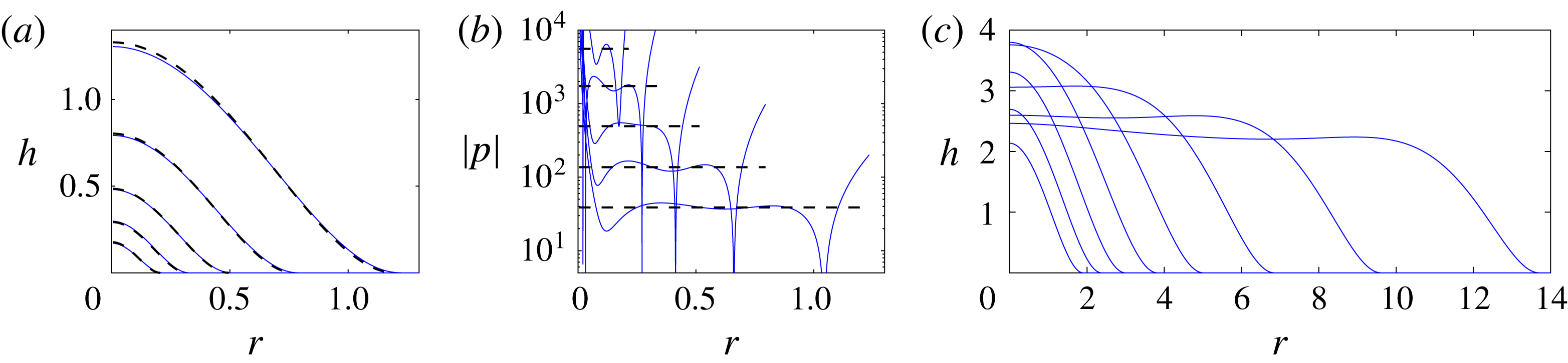
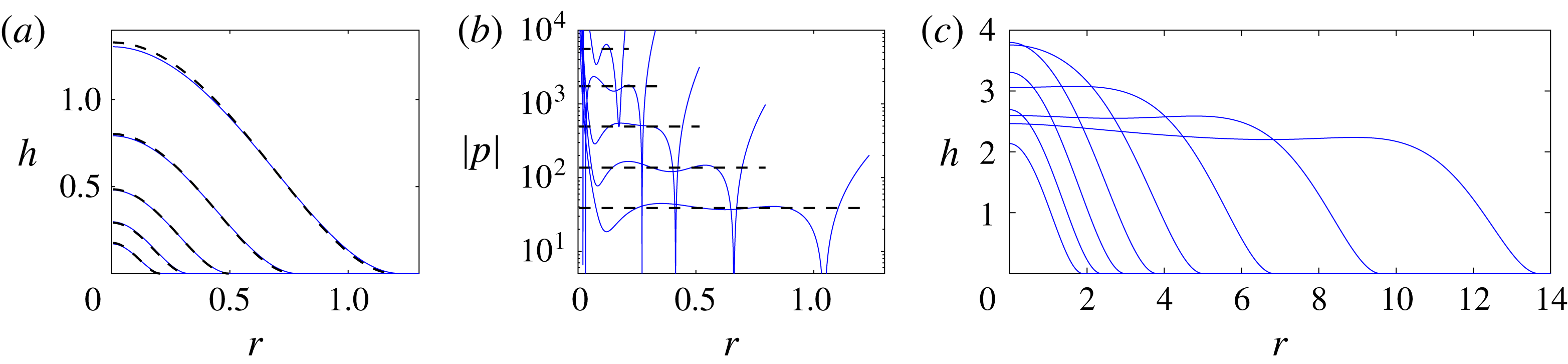
Fluid injected into the rigid till immediately creates a cavity, lifting up the overlying glacier (figure 2
a). The subsequent flow and uplift evolve through a series of regimes over time, in which the spreading of the cavity exhibits different behaviours. These are briefly outlined here. Very rapidly after injection starts (once
 $h^{3}>O(Da)$
), the majority of injected fluid flows through the cavity rather than the till. In this situation, the dominant resistance to flow comes from the flow in the vicinity of the touchdown point or nose (
 $r=R(t)$
), where the cavity narrows and propagation is driven by peeling up the overlying glacier and sucking fluid out of the porous till beneath. The majority of the radial pressure drop therefore occurs across this peeling region, and the pressure over the rest of the cavity is almost uniform (see figure 2(b); cf. Lister et al.
Reference Lister, Peng and Neufeld2013, Hewitt et al.
Reference Hewitt, Balmforth and De Bruyn2015b
).
Until the cavity grows sufficiently large, elastic bending stresses from the overlying glacier dominate the pressure gradient everywhere. Once
 $R>O(1)$
, however, gravitational forces play a role in the spreading: first, gravity affects the shape of the cavity while peeling by bending at the nose still controls the spreading rate; then, for
 $R\gg 1$
, the pressure drop is dominated by viscous losses over the whole the cavity, which subsequently evolves like a classical viscous gravity current (figure 2
c; cf. Huppert Reference Huppert1982).
In this paper, we will focus predominantly on the evolution of the cavity before gravity plays a role (i.e. when
 $R<O(1)$
), when bending by peeling at the nose controls its spread. The evolution at very early times, when the flow is largely within the porous till, is discussed in § 4.1.
3.1 A fixed flux
Once
 $h^{3}>O(Da)$
, which occurs very rapidly since
 $Da\ll 1$
, the pressure drop is largely taken up by peeling at the nose
 $r=R(t)$
. Thus the pressure over the cavity is roughly uniform (figure 2
b), such that the flux through the cavity is small and the height adopts a quasi-static profile. Given that the pressure is dominated by bending stresses from the overlying glacier,
 $p\approx \unicode[STIX]{x1D6FB}^{4}h$
from (2.4)–(2.5), which can be integrated four times to give the quasi-static profile
 $$\begin{eqnarray}h\approx \frac{3V^{\ast }}{\unicode[STIX]{x03C0}R^{2}}\left(1-\frac{r^{2}}{R^{2}}\right)^{2},\end{eqnarray}$$
where
 $V^{\ast }\approx \tilde{V}=\tilde{Q}t$
is the volume of fluid in the cavity. As the uplift approaches the nose, (3.2) is locally quadratic with curvature
 $\unicode[STIX]{x1D705}\sim \tilde{V}/R^{4}$
, which matches to the peeling profile at the nose.
Snapshots for injection at a constant flux
 $\tilde{Q}=1$
into a rigid medium, with
 $Da=1\times 10^{-9}$
. (a,c) The height profile
 $h(r,t)$
at times (a) separated by powers of four between
 $t=2^{-7}$
and
 $t=2$
, and (c) separated by powers of two between
 $t=2^{3}$
and
 $t=2^{10}$
. (b) The pressure
 $p(r,t)$
at
 $z=h$
, for the same times as in (a). The theoretical predictions for a constant-pressure cavity from (3.2) are also shown in (a) and (b) (black dashed).
This quasi-static interior profile must be matched to the peeling edge, where the radial pressure gradient is significant and drives flow in the cavity and the porous till. In the vicinity of the nose, we look for steady travelling-wave solutions to (2.13a
) moving with speed
 ${\dot{R}}$
and satisfying
 $$\begin{eqnarray}-{\dot{R}}h^{\prime }=[(h^{3}/12+Da)h^{(v)}]^{\prime },\end{eqnarray}$$
in terms of the local variable
 $x=r-{\dot{R}}t$
, where
 $^{\prime }$
denotes a derivative with respect to
 $x$
. This nose region is characterised by vertical and horizontal length scales
 $h\sim Da^{1/3}$
and
 $x\sim (Da/{\dot{R}})^{1/5}$
respectively, which are the height at which the horizontal flux through the underlying till and the cavity are comparable, and the local bending or peeling length at the tip, respectively. Given these scalings, and after integrating once,
 $$\begin{eqnarray}c-f=(f^{3}+1)f^{(v)},\end{eqnarray}$$
where
 $f=f(\unicode[STIX]{x1D709})=h(12Da)^{-1/3}$
,
 $\unicode[STIX]{x1D709}=x(Da/{\dot{R}})^{-1/5}$
and
 $c$
is a constant of integration that gives the flux across the contact radius
 $\unicode[STIX]{x1D709}=0$
. Since the till is an unbounded rigid medium ahead of the cavity, there is no leakage flux and we must set
 $c=0$
. In order to match to the quadratic behaviour of the cavity (3.2) at the nose, we solve (3.4) subject to
 $f\sim A\unicode[STIX]{x1D709}^{2}/2$
as
 $\unicode[STIX]{x1D709}\rightarrow -\infty$
, for some curvature
 $A$
, and
 $f=f^{\prime }=f^{\prime \prime }=0$
at
 $\unicode[STIX]{x1D709}=0$
. Numerical solution of this eigenvalue problem gives
 $A\approx 1.58$
.
The speed of the nose then follows from a balance of curvature between the nose and the cavity,
 $$\begin{eqnarray}{\dot{R}}=\left(\frac{\unicode[STIX]{x1D705}}{A}\right)^{5/2}\left(\frac{Da}{12^{5}}\right)^{1/6},\end{eqnarray}$$
where
 $\unicode[STIX]{x1D705}=24\tilde{V}/\unicode[STIX]{x03C0}R^{4}$
is the curvature of the cavity as it approaches the nose. Thus, for a constant flux,
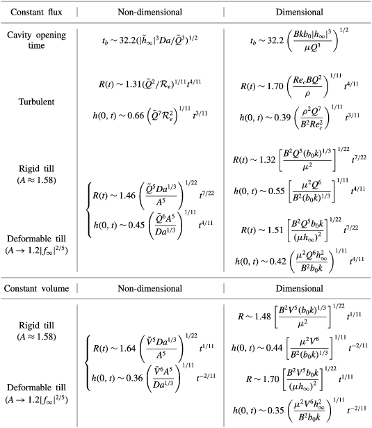
 $$\begin{eqnarray}R(t)\approx 1.46\left(\frac{\tilde{Q}^{5}Da^{1/3}}{A^{5}}\right)^{1/22}t^{7/22},\quad h(r=0,t)\approx 0.45\left(\frac{\tilde{Q}^{6}A^{5}}{Da^{1/3}}\right)^{1/11}t^{8/22},\end{eqnarray}$$
with
 $A=1.58$
. Note that, up to the value of the prefactor, these predictions are essentially the same as solutions for flow over an impermeable base with a pre-wetted film (Lister et al.
Reference Lister, Peng and Neufeld2013), with the film thickness in that situation being replaced by the local height scale
 ${\sim}Da^{1/3}$
of the nose. Accordingly, the solutions have an extraordinarily weak dependence on
 $Da$
, with
 $R\sim Da^{1/66}t^{7/22}$
. The fluid spreads effectively independently of the permeability of the base, provided that the permeability is small (but, crucially, non-zero).
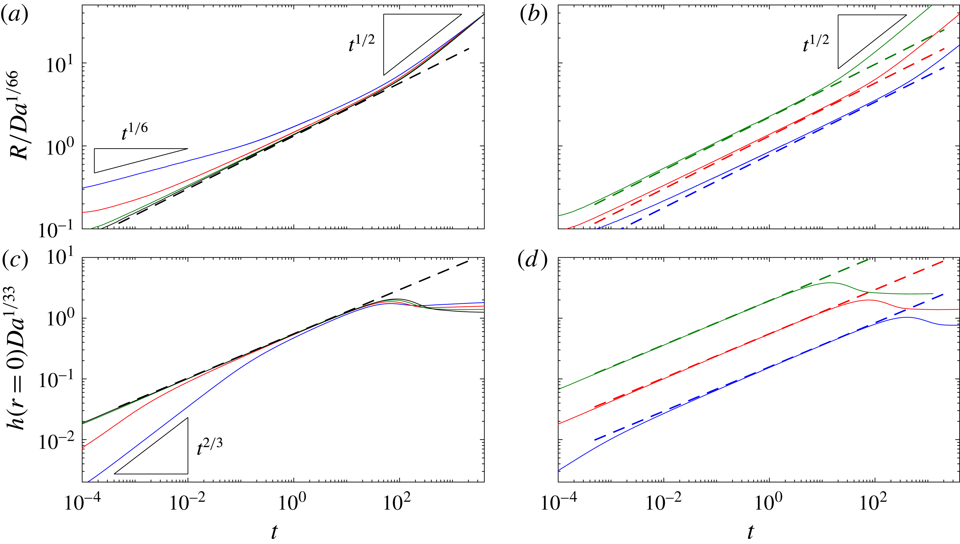
Data from computations with a rigid till and constant injection flux, showing (a,b) the scaled position of the nose
 $R(t)/Da^{1/66}$
, and (c, d) the scaled height of the uplift at the origin
 $h\,Da^{1/33}$
. (a,c) Solutions for
 $Da=10^{-3}$
(blue),
 $Da=10^{-5}$
(red),
 $Da=10^{-7}$
(green) and
 $Da=10^{-9}$
(black), all with
 $\tilde{Q}=1$
. (b,d) Solutions for
 $\tilde{Q}=0.1$
(blue),
 $\tilde{Q}=1$
(red) and
 $\tilde{Q}=10$
(green), all with
 $Da=10^{-7}$
. The dashed lines show the predictions in (3.6). At very early times, the flow is dominated by flow through the porous till and
 $R\sim (Da\,t)^{1/6}$
(see § 4.1). For
 $R\gg 1$
, gravity affects the dynamics and the flow spreads like a classical gravity current with
 $R\sim t^{1/2}$
.
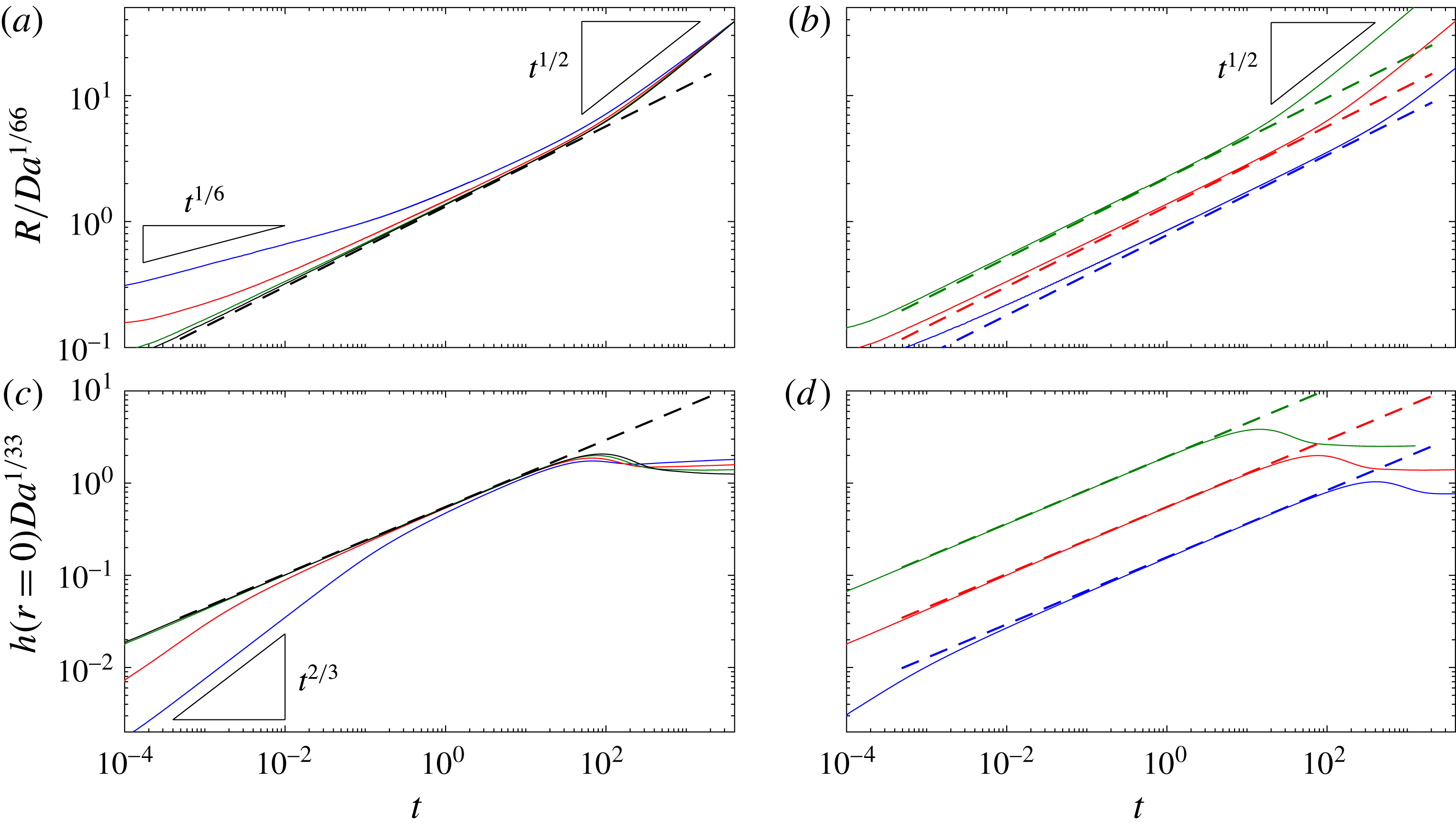
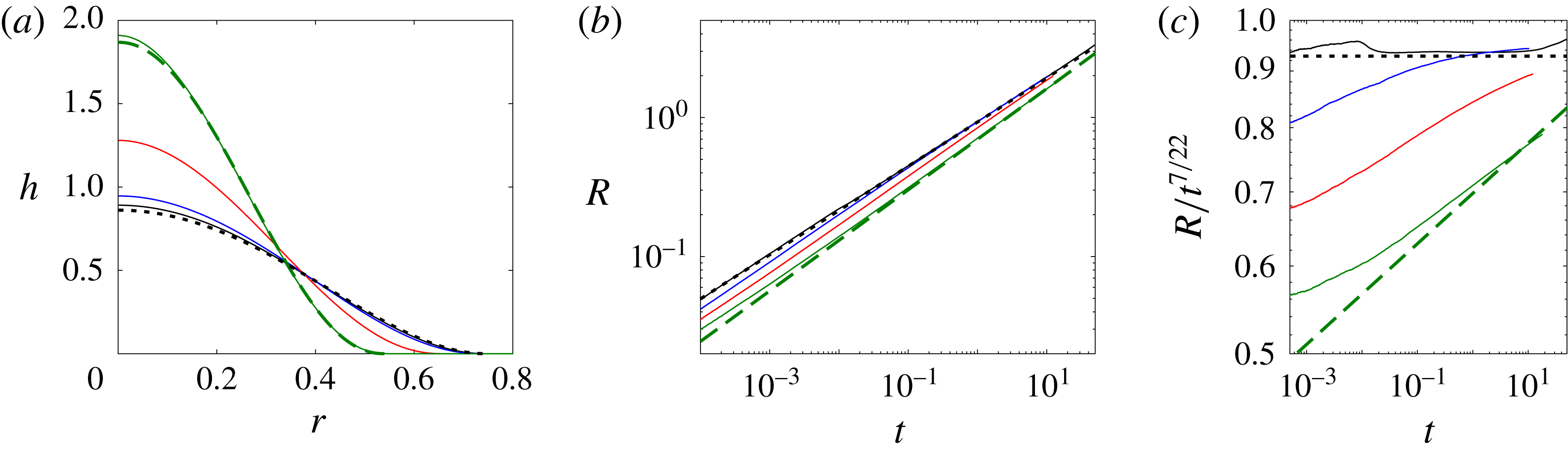
Figure 3 shows a selection of data from numerical simulations which verify the predictions in (3.6). The predictions give excellent agreement when
 $Da$
is small, as in the relevant geophysical limit, although the numerical solutions suggest a slightly stronger dependence on
 $Da$
than that in (3.6) when
 $Da$
is relatively large. This discrepancy arises because the assumption of a constant-pressure cavity breaks down in this limit: if
 $Da$
is too large there is only weak resistance to peeling at the nose; both length and height scales of the travelling-wave solution,
 ${\sim}Da^{1/5}/{\dot{R}}$
and
 ${\sim}Da^{1/3}$
, become large, and the pressure drop can no longer be assumed to be localised to the nose.
As discussed at the start of this section, once the current has spread to a radius
 $R>O(1)$
, the gradient in hydrostatic pressure across the current becomes comparable to the pressure drop across the nose. For intermediate times, bending stresses associated with peeling at the nose still dominate the pressure gradient, but gravity enters the pressure balance over the quasi-static cavity, which results in a different expression in (3.2), and leads to a prediction
 $R\sim t^{7/12}$
and
 $h(r=0)\sim t^{-1/6}$
in (3.6) (cf. Lister et al.
Reference Lister, Peng and Neufeld2013). At later times, the viscous losses associated with the flow across the cavity become so large that the spreading becomes dominated by gravity, except in the vicinity of the nose and around the origin where bending stresses continue to play a role. The cavity then spreads like a viscous gravity current with
 $R\sim t^{1/2}$
and
 $h(r=0)$
roughly constant. This ultimate transition can be observed clearly in the snapshots of figure 2(c).
3.2 A fixed volume
If the flux
 $\tilde{Q}$
is stopped at some time
 $t_{v}$
, the injected volume of fluid
 $\tilde{V}=\tilde{Q}t_{v}$
continues to spread, as would be the case for the rapid drainage of a finite volume supraglacial lake. The travelling-wave solution at the nose in this case is identical to the previous section, but now the integral of (3.5) indicates the cavity spreads according to
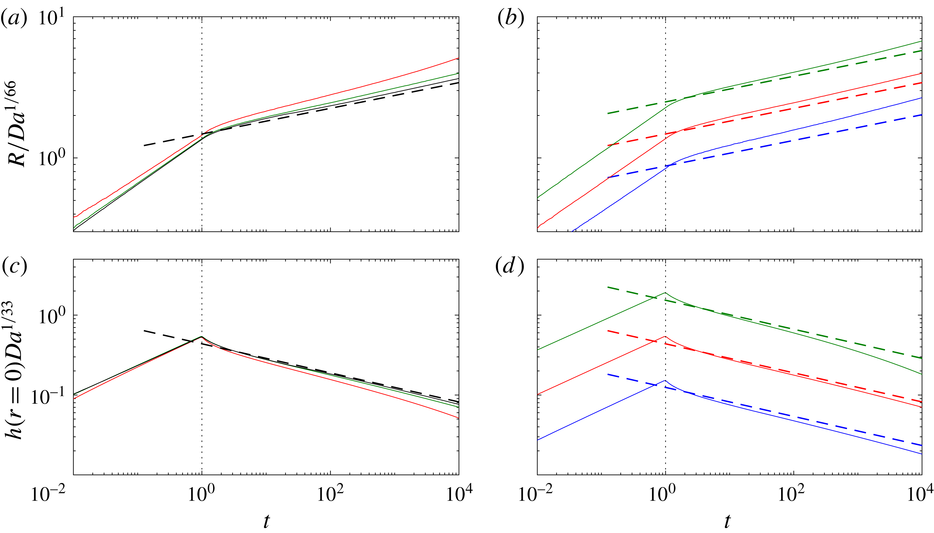
 $$\begin{eqnarray}R(t)\approx 1.64\left(\frac{\tilde{V}^{5}Da^{1/3}}{A^{5}}\right)^{1/22}t^{1/11};\quad h(r=0,t)\approx 0.36\left(\frac{\tilde{V}^{6}A^{5}}{Da^{1/3}}\right)^{1/11}t^{-2/11},\end{eqnarray}$$
where, again,
 $A\approx 1.58$
. As in (3.6), the dependence on
 $Da$
is effectively negligibly weak. Note that the radius of the cavity continues to spread, but much more slowly, while the height at the origin drops.
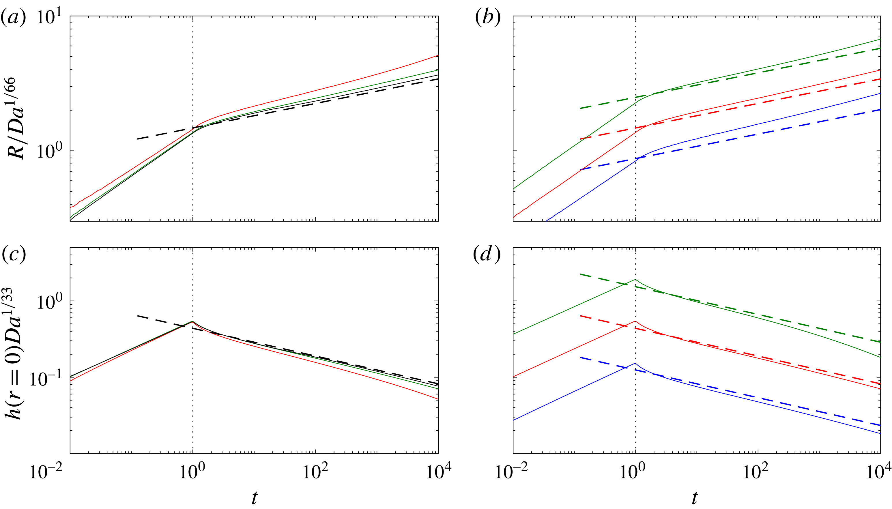
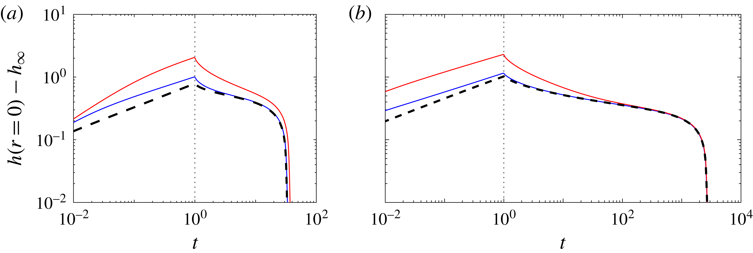
Figure 4 shows data from numerical simulations in which a constant flux of fluid is injected up to
 $t=1$
, followed by the slumping of a constant volume of fluid. As expected, the model again gives increasingly good agreement as
 $Da$
is made smaller (figure 4
a,c). Over time, and for smaller volumes of fluid, there is a weak drift from the asymptotic prediction, which arises as the length scale of the nose region
 ${\sim}(Da/{\dot{R}})^{1/5}$
grows. Results for larger volumes of fluid also deviate from the asymptotic predictions (figure 4
b,d), as the radius more rapidly grows to a size large enough for gravity to affect the flow.
In summary, spreading with either a fixed flux or fixed volume is made possible by the presence of an underlying saturated porous medium, but for a rigid till the dependence of the propagation rate on the properties of the media in each case is negligibly weak.
Data from computations with a rigid till showing the spread of a fixed volume with
 $t_{v}=1$
. (a,b) The scaled position of the nose
 $R(t)/Da^{1/66}$
, and (c,d) the scaled height of the uplift at the origin
 $h\,Da^{1/33}$
. (a,c) Solutions for
 $Da=10^{-5}$
(red),
 $Da=10^{-7}$
(green) and
 $Da=10^{-9}$
(black), all with
 $\tilde{Q}=\tilde{V}=1$
. (b,d) Solutions for
 $\tilde{Q}=\tilde{V}=0.1$
(blue),
 $\tilde{Q}=\tilde{V}=1$
(red) and
 $\tilde{Q}=\tilde{V}=10$
(green), all with
 $Da=10^{-7}$
. The dashed lines show the predictions in (3.7). The vertical dotted line signifies
 $t=t_{v}$
, when the injection flux is set to zero.
4 Deformable till
The case of a rigid till is given by the joint limit
 $\tilde{h}_{\infty }\rightarrow 0$
and
 $\tilde{M}\rightarrow \infty$
. If the till is not perfectly rigid but is instead initially compressed to some height
 $\tilde{h}_{\infty }<0$
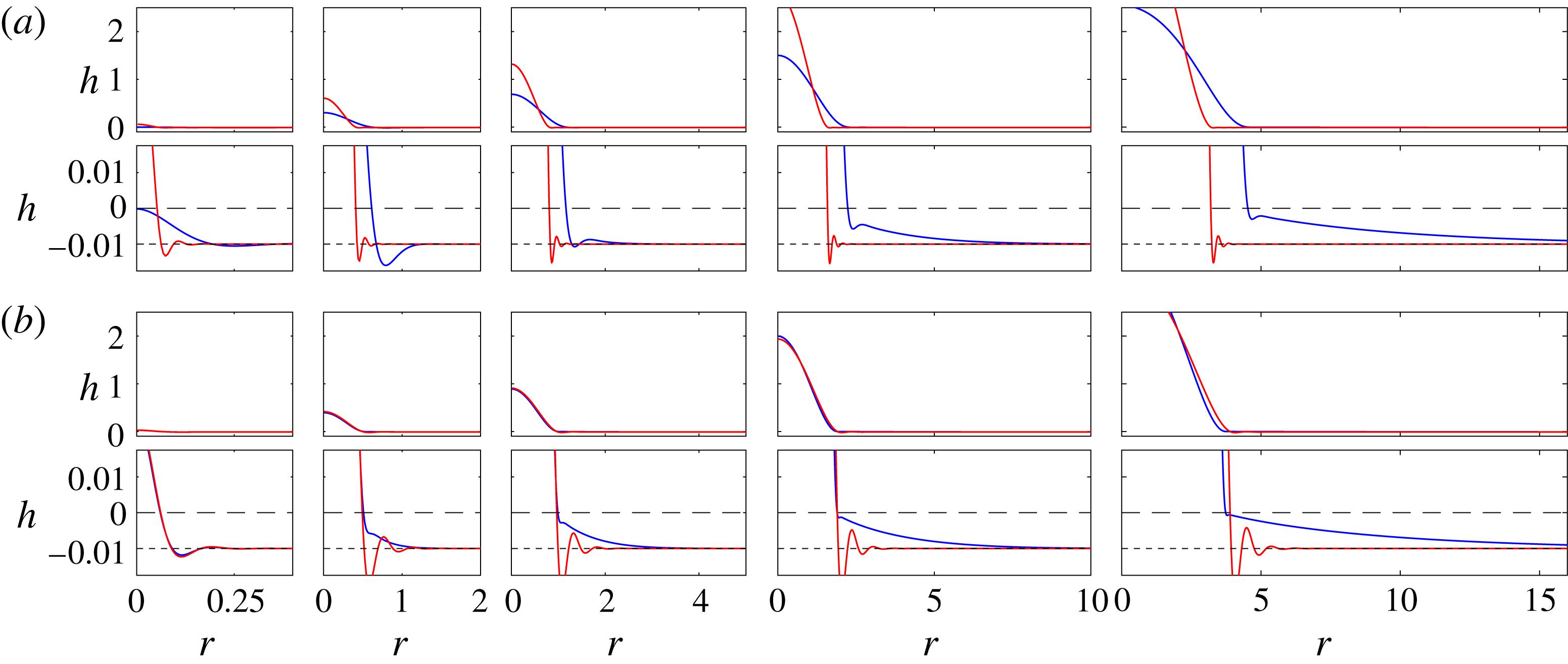
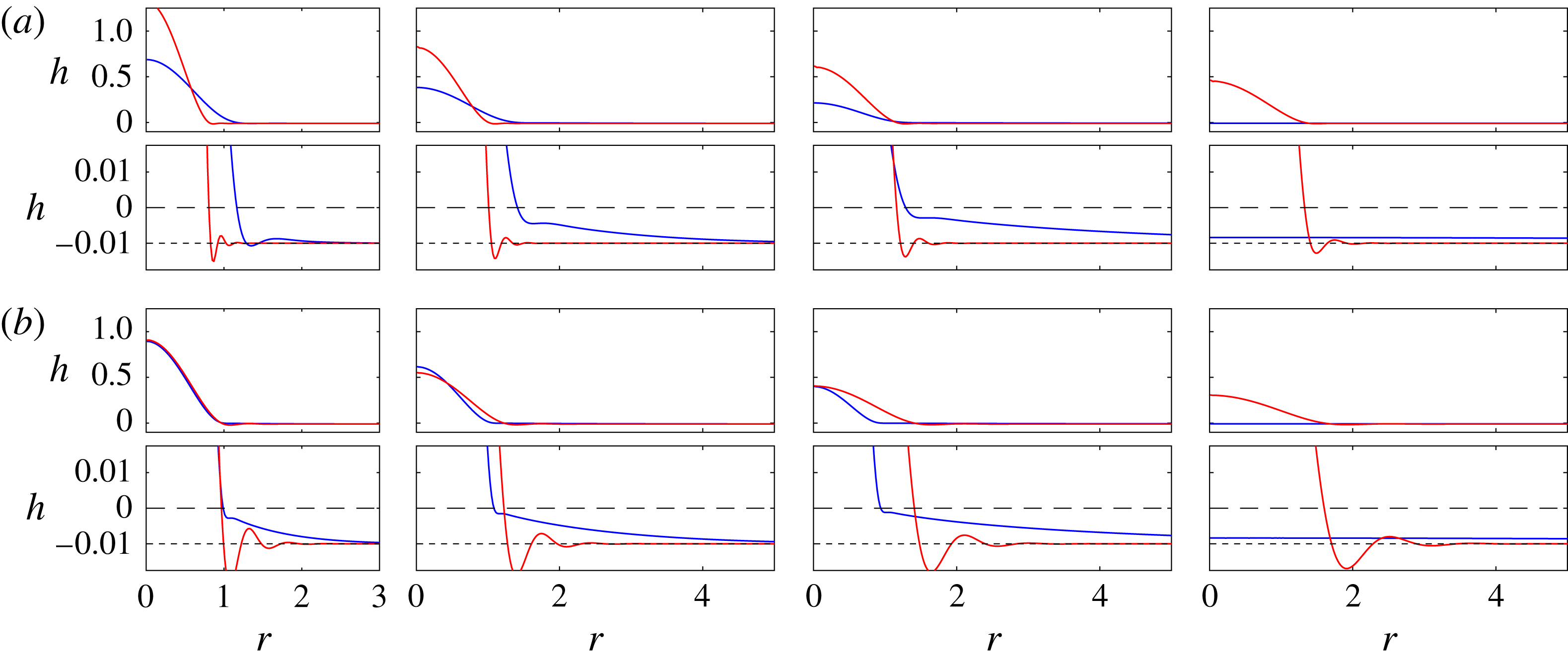
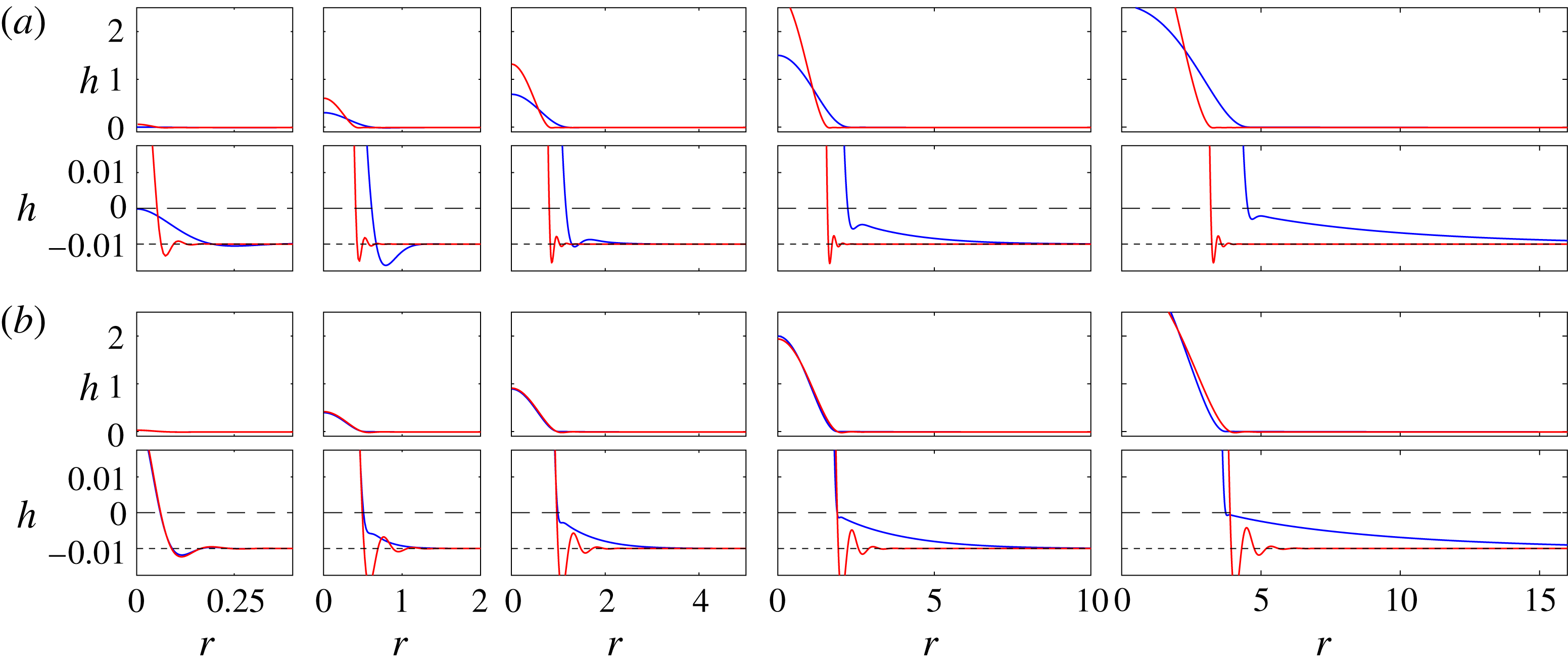
, the deformation in the till must be coupled with the uplift of the glacier. We begin this section by presenting some snapshots (figure 5) from numerical solutions to motivate the subsequent analysis. When the till is deformable, a fluid-filled cavity does not immediately form; instead, fluid initially flows into the till, causing it to expand as the increased fluid pressure reduces the load on the matrix (e.g. first panel in figure 5
a). In general, after some time the till becomes fully saturated near the injection point, and the glacier lifts off the base as fluid flows into a cavity above the till. The subsequent spread of the cavity is qualitatively similar to flow above a rigid base, except that the deformation of the till ahead of the nose can affect its spread. Figure 5 demonstrates two different behaviours: for small till permeability,
 $Da$
, or small till stiffness,
 $\tilde{M}$
, the deformation signal can remain localised to the nose, taking the form of an oscillatory bending wave, while for larger
 $Da$
or
 $\tilde{M}$
, deformation appears to propagate increasingly far ahead of the nose. The qualitative effect of the deformation ahead of the nose on the spread of the cavity is not immediately clear: in figure 5(a) the solution with more localised deformation at the nose lags behind the other, while in figure 5(b) it spreads very slightly ahead.
We explore this behaviour in the following subsections. We begin in § 4.1 by describing the initial spread when the majority of fluid flows through the till and, in § 4.2, the subsequent spreading in the till ahead of the cavity. We then examine in some detail the spread of the cavity, driven by peeling at its nose.
Snapshots of the uplift
 $h(r,t)$
from numerical solutions with
 $\tilde{Q}=1$
, and
 $\tilde{h}_{\infty }=-10^{-2}$
, for different parameters representing relatively high or low values of the till permeability and stiffness. Profiles are shown in each panel at times, from left to right,
 $t=2^{-12}$
,
 $t=2^{-3}$
,
 $t=1$
,
 $t=2^{3}$
and
 $t=2^{6}$
. Lower panels show an enlarged version of the same data, to reveal the form of the uplift in the till; black lines show
 $z=0$
(long dashed) and
 $z=\tilde{h}_{\infty }$
(short dashed) for reference. (a) ‘High’ permeability (
 $Da=10^{-3}$
, blue) and ‘low’ permeability (
 $Da=10^{-8}$
, red), each with
 $\tilde{M}=10^{4}$
. (b) ‘High’ stiffness (
 $\tilde{M}=10^{6}$
, blue) and ‘low’ stiffness (
 $\tilde{M}=10^{2}$
, red), each with
 $Da=10^{-6}$
.
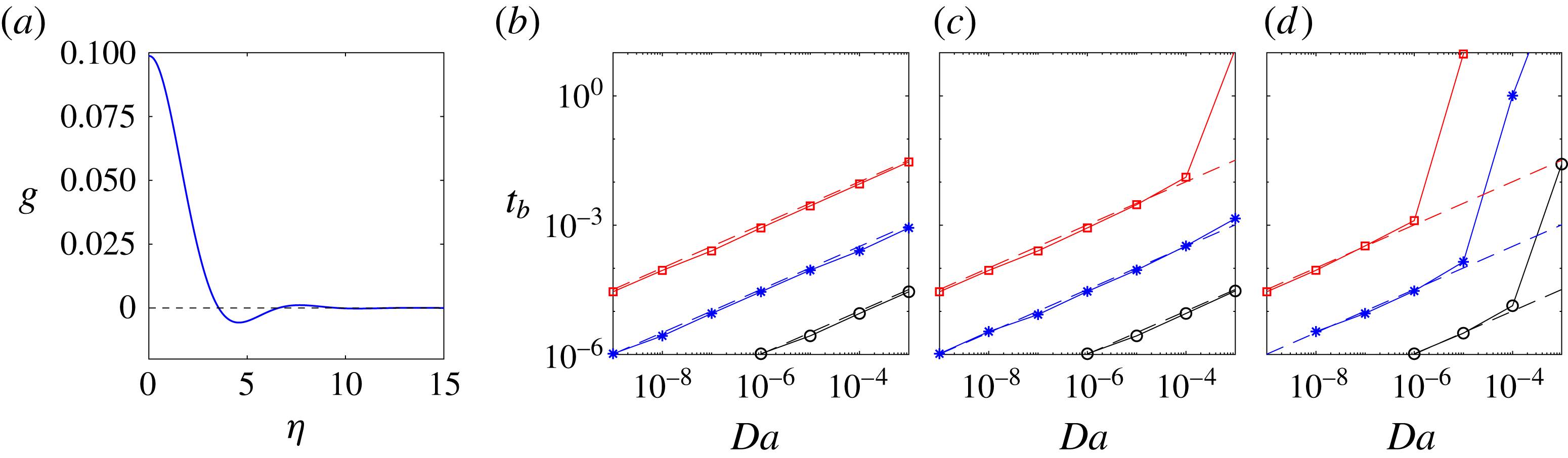
4.1 Initial uplift from a poroelastic till
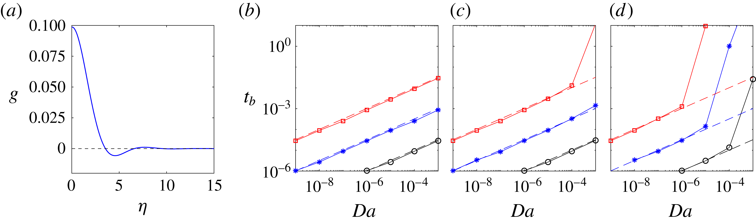
(a) The similarity solution
 $g(\unicode[STIX]{x1D702})$
for the initial uplift, from (4.2). (b–d) The time
 $t_{b}$
at which the glacier first lifts off the base, extracted from numerical computations with
 $\tilde{Q}=1$
, as a function of
 $Da$
and for stiffness (b)
 $\tilde{M}=10^{2}$
, (c)
 $\tilde{M}=10^{4}$
and (d)
 $\tilde{M}=10^{6}$
. The initial compression of the till is
 $\tilde{h}_{\infty }=-10^{-3}$
(black circles),
 $\tilde{h}_{\infty }=-10^{-2}$
(blue stars) and
 $\tilde{h}_{\infty }=-10^{-1}$
(red squares). Dashed lines show the asymptotic prediction
 $t_{b}\approx 32.2(|\tilde{h}_{\infty }|^{3}Da/\tilde{Q}^{3})^{1/2}$
, which is independent of
 $\tilde{M}$
but breaks down if
 $Da\,\tilde{M}|\tilde{h}_{\infty }|/\tilde{Q}$
is sufficiently large (see (4.5)).
Fluid initially flows into the pore spaces in the compressed till. After some time
 $t=t_{b}$
, the till in the vicinity of
 $r=0$
becomes saturated and the glacier is lifted up by the formation of a fluid-filled cavity. Up until this time, the flow is governed by (2.13b
) and (2.16), and, provided the radial extent of the flow remains small, is dominated by the bending stresses from the overlying glacier, rather than by gravity or the elasticity of the till. The dominant balances in those equations are thus
 $h/t\sim Da\,h/r^{6}$
, which describes fluid and pore-pressure diffusion under an elastic membrane, and
 $\tilde{Q}t\sim r^{2}(h-\tilde{h}_{\infty })$
.
Assuming the injection flux is constant, these scalings motivate the search for an early-time similarity solution of the form
 $$\begin{eqnarray}h=\tilde{h}_{\infty }+\frac{\tilde{Q}\,t^{2/3}}{Da^{1/3}}g(\unicode[STIX]{x1D702});\quad \unicode[STIX]{x1D702}\equiv \frac{r}{(Da\,t)^{1/6}}.\end{eqnarray}$$
The solution
 $g(\unicode[STIX]{x1D702})$
satisfies the sixth-order ordinary differential equation (ODE)
 $$\begin{eqnarray}\frac{2}{3}g-\frac{1}{6}\unicode[STIX]{x1D702}\frac{\unicode[STIX]{x2202}g}{\unicode[STIX]{x2202}\unicode[STIX]{x1D702}}=\frac{1}{\unicode[STIX]{x1D702}}\frac{\unicode[STIX]{x2202}}{\unicode[STIX]{x2202}\unicode[STIX]{x1D702}}\left[\unicode[STIX]{x1D702}\frac{\unicode[STIX]{x2202}}{\unicode[STIX]{x2202}\unicode[STIX]{x1D702}}\left(\frac{1}{\unicode[STIX]{x1D702}}\frac{\unicode[STIX]{x2202}}{\unicode[STIX]{x2202}\unicode[STIX]{x1D702}}\unicode[STIX]{x1D702}\frac{\unicode[STIX]{x2202}}{\unicode[STIX]{x2202}\unicode[STIX]{x1D702}}\right)^{2}g\right],\end{eqnarray}$$
together with
 $g^{\prime }=g^{\prime \prime \prime }=0$
at
 $\unicode[STIX]{x1D702}=0$
,
 $g=g^{\prime \prime }=g^{\prime \prime \prime }=0$
as
 $\unicode[STIX]{x1D702}\rightarrow \infty$
and
 $2\unicode[STIX]{x03C0}\int _{0}^{\infty }\unicode[STIX]{x1D702}g\,\text{d}\unicode[STIX]{x1D702}=1$
. Numerical solution of this ODE (figure 6
a) shows that the uplift decays away from the origin and exhibits strongly damped oscillations about
 $g=0$
(
 $h=\tilde{h}_{\infty }$
).
A cavity will form above the till once the height rises to
 $h=0$
, which is when the effective solid stress has dropped to zero and the till is fully saturated. The highest uplift is evidently at the origin (see solution in figure 6
a), and the numerical solution gives
 $g\rightarrow 0.0988$
as
 $\unicode[STIX]{x1D702}\rightarrow 0$
. This value, from (4.1), gives
 $h=0$
when
 $$\begin{eqnarray}t_{b}\approx 32.2\left(\frac{|\tilde{h}_{\infty }|^{3}Da}{\tilde{Q}^{3}}\right)^{1/2}.\end{eqnarray}$$
This prediction for the lift-off time
 $t_{b}$
is independent of the stiffness of the till, and gives good agreement with numerical results over a range of parameter space (figure 6). The prediction breaks down, however, if the radial scale of the flow
 ${\sim}(Da\,t)^{1/6}$
becomes comparable to the length scale at which stiffness in the till balances the bending stresses,
 ${\sim}\tilde{M}^{-1/4}$
, before the till is fully saturated; i.e. if
 $$\begin{eqnarray}t_{b}\gtrsim t_{s}\equiv \frac{1}{\tilde{M}^{3/2}Da},\end{eqnarray}$$
or
 $$\begin{eqnarray}\frac{|\tilde{h}_{\infty }|Da\tilde{M}}{\tilde{Q}}\gtrsim O(0.1).\end{eqnarray}$$
If (4.5) holds, the flow in the till changes to a classical poroelastic diffusive current and spreads much more rapidly (
 $r\sim t^{1/2}$
, as discussed in § 4.2 below). This transition will therefore significantly delay the formation of a cavity, as can be seen in the data from simulations in figure 6.
4.2 Deformation in the till
Once
 $t\gtrsim t_{s}$
, as defined in (4.4), the stiffness of the till, rather than the bending stress of the overlying ice, dominates the radial pressure gradient in the till. Irrespective of whether a cavity has formed near
 $r=0$
or not, the deformation in the till far from the origin is governed by classical poroelastic diffusion after this time, and (2.13b
) reduces to the linear diffusion equation
 $$\begin{eqnarray}\frac{\unicode[STIX]{x2202}h}{\unicode[STIX]{x2202}t}\approx \frac{Da\tilde{M}}{r}\frac{\unicode[STIX]{x2202}}{\unicode[STIX]{x2202}r}r\frac{\unicode[STIX]{x2202}h}{\unicode[STIX]{x2202}r},\end{eqnarray}$$
provided
 $\tilde{h}_{\infty }\ll 1$
and
 $\tilde{M}\gg 1$
. Equation (4.6) gives diffusive radial spreading over a length scale
 $r\sim (Da\tilde{M}\,t)^{1/2}$
, which we will return to in the following sections and thus denote by
 $X(t)$
. Subsequently, we will show that the ratio of this poroelastic deformation length
 $X\sim (Da\tilde{M}\,t)^{1/2}$
to the radius of the cavity
 $R(t)$
controls the evolution of the system.
4.3 The spread of the cavity
Once the glacier has lifted off the base and the cavity has grown large enough (
 $h^{3}>O(Da)$
), the fluid-filled cavity spreads in a manner analogous to spreading over a rigid till in § 3: peeling by bending at the nose over a narrow region of length
 $(Da/{\dot{R}})^{1/5}$
controls the spread of the roughly uniform-pressure cavity behind, which evolves quasi-statically as in (3.2). However, the details of peeling at the nose are different, and depend on the manner in which the cavity matches to deformation in the till ahead of the nose.
The matching depends crucially on whether the cavity radius
 $R(t)$
is large or small relative to the characteristic length scale
 $X(t)$
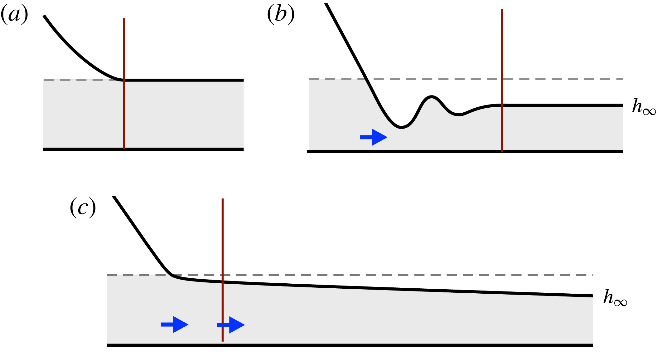
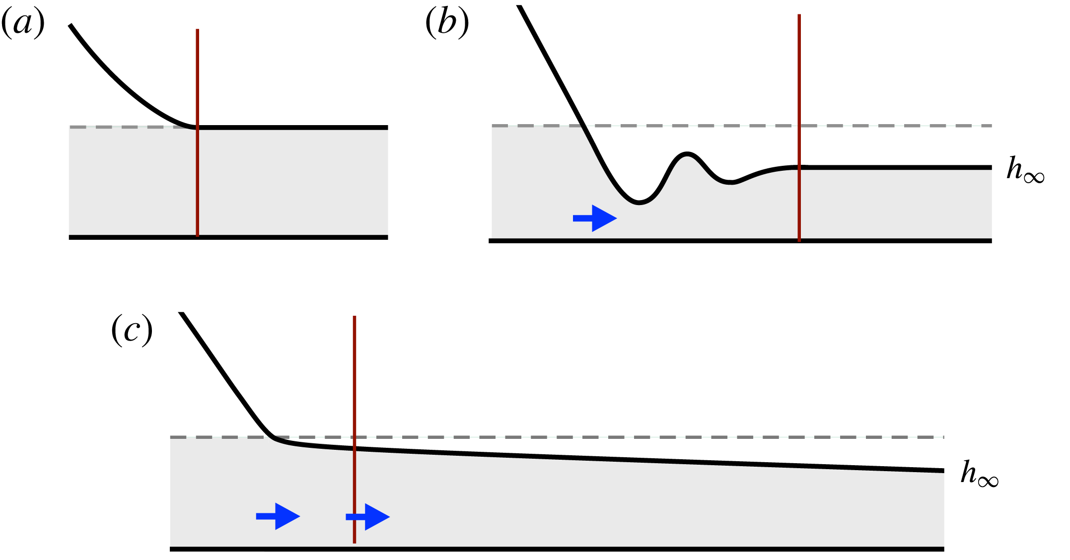
of deformation in the till discussed in § 4.2. The two cases are shown schematically in figure 7(b,c), respectively. When the cavity radius is large compared to deformation in the till,
 $R\gg X$
, there is a compact travelling-wave region around the nose which matches smoothly to an undeformed profile ahead, and propagation is by peeling. In contrast, when the deformation in the till extends over a larger region than the cavity radius,
 $X\gg R$
, the travelling-wave region matches the quasi-static cavity behind to a spreading region of deformation in the till ahead of the nose. Generically, we find that the flow evolves from the former case towards the latter, but that the influence of gravity on the flow may take hold before this transition can occur at
 $R\gtrsim 1$
.
As in § 3, the shape of the quasi-static cavity is given by (3.2), while the evolution of the nose is again described by a local travelling-wave solution,
 $$\begin{eqnarray}-{\dot{R}}h^{\prime }\approx \left\{\begin{array}{@{}ll@{}}[(h^{3}/12+Da)h^{(v)}]^{\prime }\quad & \text{if }x\leqslant 0,\\ Da[h^{(v)}+\tilde{M}h^{\prime }]^{\prime }\quad & \text{if }x>0,\end{array}\right.\end{eqnarray}$$
from (2.13), where
 $x=r-{\dot{R}}t$
, recalling that we are working in the limit
 $\tilde{M}\gg 1$
. Again, as in § 3, (4.7) can be rescaled by the vertical height scale
 $h\sim Da^{1/3}$
and local bending length
 $x\sim (Da/{\dot{R}})^{1/5}$
, and integrated to give
 $$\begin{eqnarray}c-f=\left\{\begin{array}{@{}ll@{}}(f^{3}+1)f^{(v)}\quad & \text{if }\unicode[STIX]{x1D709}\leqslant 0,\\ f^{(v)}+\unicode[STIX]{x1D6E4}^{4}f^{\prime }\quad & \text{if }\unicode[STIX]{x1D709}>0,\end{array}\right.\end{eqnarray}$$
where
 $f=f(\unicode[STIX]{x1D709})=h/(12Da)^{1/3}$
,
 $\unicode[STIX]{x1D709}=x({\dot{R}}/Da)^{1/5}$
,
 $c$
is a constant of integration that gives the flux across
 $\unicode[STIX]{x1D709}=0$
, and the new parameter
 $$\begin{eqnarray}\unicode[STIX]{x1D6E4}=\left(\frac{Da}{{\dot{R}}}\right)^{1/5}\tilde{M}^{1/4}\end{eqnarray}$$
is the ratio of the characteristic peeling length at the nose,
 $(Da/{\dot{R}})^{1/5}$
, to the length scale over which bending and stiffness balance in the till,
 $\tilde{M}^{-1/4}$
. Equation (4.8) is solved subject to
 $f\rightarrow A\unicode[STIX]{x1D709}^{2}/2$
as
 $\unicode[STIX]{x1D709}\rightarrow -\infty$
and
 $f=[f^{\prime }]=[f^{\prime \prime }]=[f^{\prime \prime \prime }]=[f^{\prime \prime \prime \prime }]=0$
at
 $\unicode[STIX]{x1D709}=0$
, for some curvature
 $A(c,\unicode[STIX]{x1D6E4})$
. The conditions as
 $\unicode[STIX]{x1D709}\rightarrow \infty$
depend on the spatial form of the deformation ahead of the nose, as discussed below.
Once again, the curvature
 $A(c,\unicode[STIX]{x1D6E4})$
determines the spreading rate
 ${\dot{R}}$
via (3.5). Given
 $A$
, the radius
 $R(t)$
and height
 $h(r=0)$
are exactly as in (3.6). However, unlike for (3.4), the flux
 $c$
is not, in general, zero. Instead
 $c$
, and the solution
 $f(\unicode[STIX]{x1D709})$
, are determined by matching to the deformation in the till as
 $\unicode[STIX]{x1D709}\rightarrow \infty$
.
Schematics of the travelling-wave region around the nose for (a) a rigid till, (b) a deformable till with
 $R\gg X$
(here drawn with
 $\unicode[STIX]{x1D6E4}\ll 1$
; see (4.9) and § 4.3.1) and (c) a deformable till with
 $R\ll X$
, where
 $X=(Da\,\tilde{M}\,t)^{1/2}$
is the length scale of poroelastic deformation in the till and
 $R$
is the radius of the cavity. The grey shaded regions denote the till, the vertical lines indicate the right-hand edge of the travelling-wave region, while the thick blue arrows denote the flux of fluid. Only in (c) does fluid spread ahead of the travelling-wave region.
We note here that, given
 $c$
as discussed in the following subsections, the true (unscaled) flux through the nose, which we label
 $q_{R}$
, can be determined by reversing the scalings that yielded (4.8) and integrating around the fixed radius
 $r=R$
to give
 $$\begin{eqnarray}q_{R}=-2\unicode[STIX]{x03C0}R\,c\,{\dot{R}}(12Da)^{1/3}.\end{eqnarray}$$
4.3.1 Compact response:
 $R\gg X$

When the length scale of deformation in the poroelastic till is small compared with the cavity radius,
 $R\gg X=(Da\,\tilde{M}\,t)^{1/2}$
, the travelling-wave solution matches smoothly to
 $h=\tilde{h}_{\infty }$
ahead, as the cavity overruns the characteristic diffusion of pressure in the till. In scaled variables,
 $f\rightarrow f_{\infty }$
as
 $\unicode[STIX]{x1D709}\rightarrow \infty$
, where
 $$\begin{eqnarray}f_{\infty }=\frac{\tilde{h}_{\infty }}{(12Da)^{1/3}},\end{eqnarray}$$
and so
 $c=f_{\infty }$
from (4.8b
).
It is evident from the form of (4.8) that solutions will depend on the size of
 $\unicode[STIX]{x1D6E4}$
. In the limit of a ‘soft’ till,
 $\unicode[STIX]{x1D6E4}\ll 1$
, the stiffness length scale is much greater than the bending scale at the nose, and (4.8) reduces to
 $$\begin{eqnarray}f_{\infty }-f=\left\{\begin{array}{@{}ll@{}}(f^{3}+1)f^{(v)}\quad & \text{if }\unicode[STIX]{x1D709}\leqslant 0,\\ f^{(v)}\quad & \text{if }\unicode[STIX]{x1D709}>0,\end{array}\right.\end{eqnarray}$$
with boundary conditions as for (4.8), and
 $f^{\prime },\,f^{\prime \prime }\rightarrow 0$
as
 $\unicode[STIX]{x1D709}\rightarrow \infty$
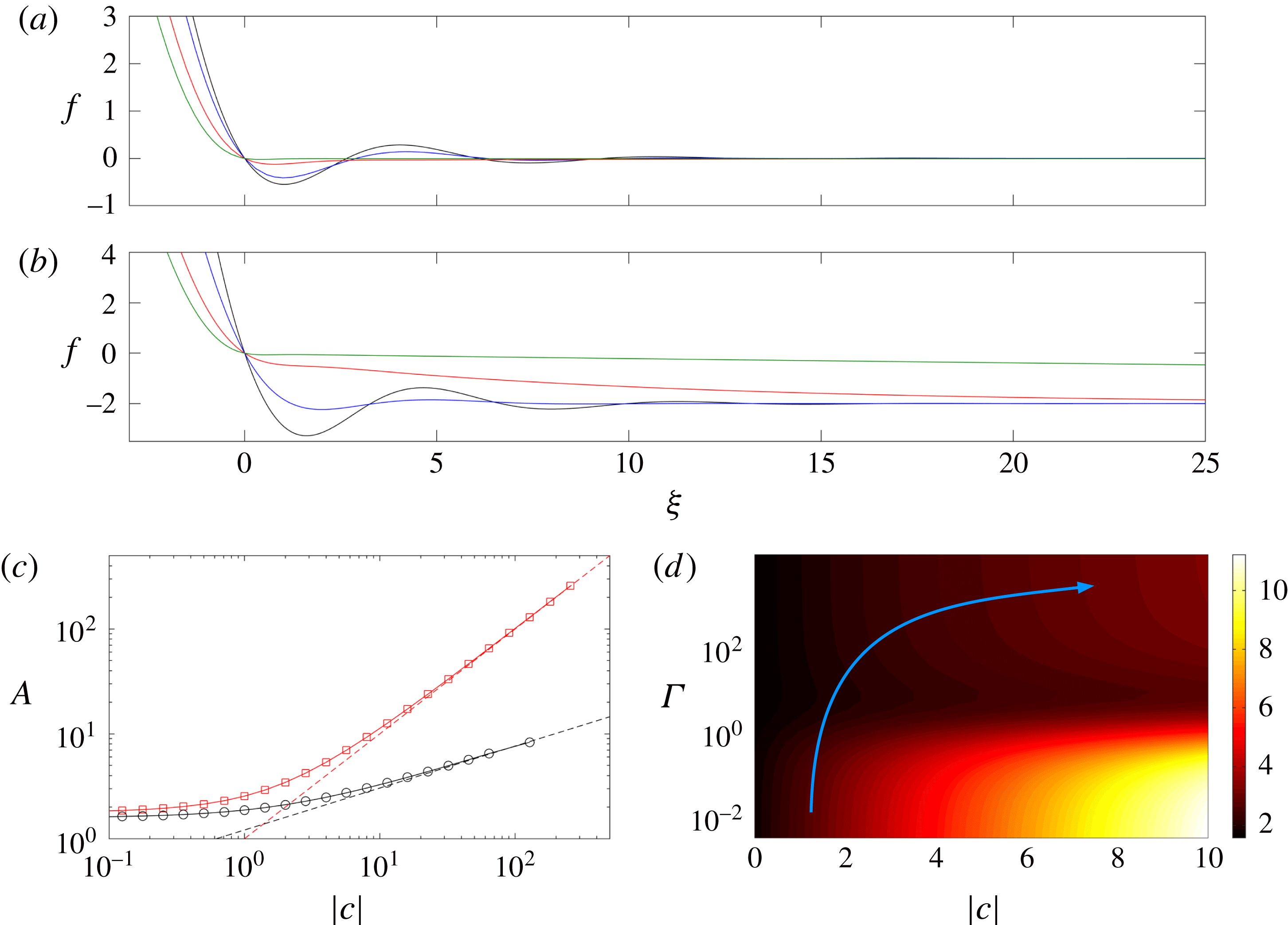
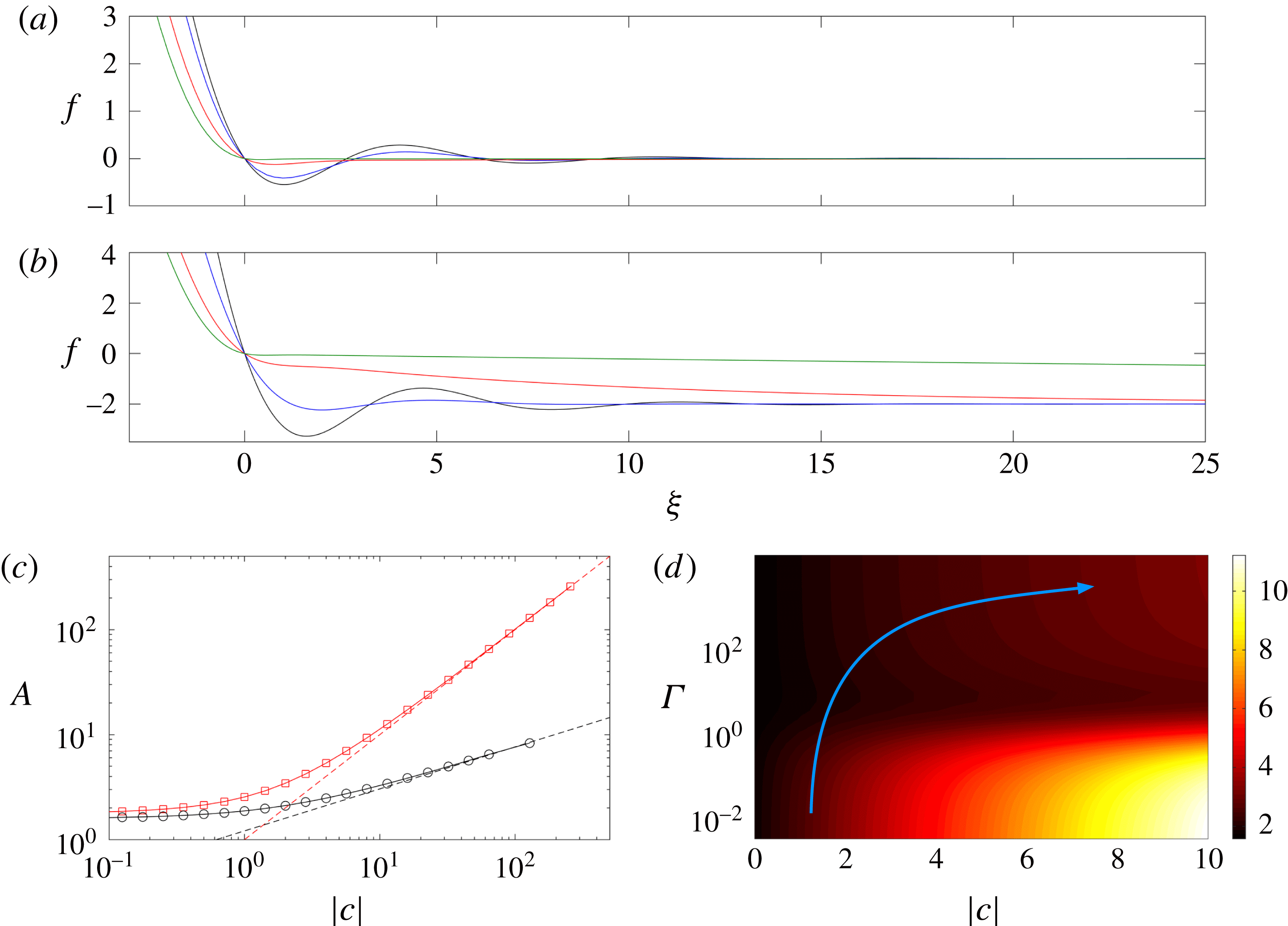
. Solutions of (4.12) take the form of a damped oscillatory bending wave ahead of the nose (see solutions with small
 $\unicode[STIX]{x1D6E4}$
in figure 8
a,b). The curvature
 $A$
that matches to the cavity increases with
 $f_{\infty }$
(figure 8
c) and has a limiting value
 $A\rightarrow 1.78$
as
 $f_{\infty }\rightarrow 0$
. For large
 $|\,f_{\infty }|$
, the relevant height scale of the solutions changes and an asymptotic analysis in this limit gives
 $A\rightarrow |f_{\infty }|$
(figure 8
c).
(a,b) Solutions of the travelling-wave equation (4.8) in the limit
 $R\gg X=(Da\,\tilde{M}\,t)^{1/2}$
, such that the travelling wave matches smoothly to
 $\tilde{h}_{\infty }$
ahead. (a)
 $f_{\infty }=0$
, and (b)
 $f_{\infty }=-2$
, with
 $\unicode[STIX]{x1D6E4}=0$
(black),
 $\unicode[STIX]{x1D6E4}=1$
(blue),
 $\unicode[STIX]{x1D6E4}=10^{1/4}$
(red) and
 $\unicode[STIX]{x1D6E4}=100^{1/4}$
(green). (c) The curvature
 $A=f^{\prime \prime }(\unicode[STIX]{x1D709}\rightarrow -\infty )$
of the travelling-wave profile, as a function of the scaled flux
 $c$
, in the soft-till limit
 $\unicode[STIX]{x1D6E4}=0$
(red squares) and in the rigid-till limit
 $\unicode[STIX]{x1D6E4}\rightarrow \infty$
(black circles). The dashed lines show the asymptotic predictions for large
 $c$
:
 $A\rightarrow |c|$
and
 $A\rightarrow 1.2|c|^{2/5}$
. (d) A density map of the curvature
 $A(c,\unicode[STIX]{x1D6E4})$
, calculated from (4.8) for different
 $\unicode[STIX]{x1D6E4}$
and
 $c$
. Recall that
 $c$
evolves between the two limits
 $c=f_{\infty }=\tilde{h}_{\infty }/(12Da)^{1/3}$
for
 $R\gg X$
and (4.20) for
 $R\ll X$
. The blue arrow sketches a typical trajectory of the curvature over time (see § 4.4).
In the opposite limit of a ‘stiff’ till,
 $\unicode[STIX]{x1D6E4}\gg 1$
, the uplift ahead of the nose is dominated by relaxation of the network stress – that is, the effective solid stress – in the till. In this limit, based on the form of (4.8) we expect a narrow boundary layer of width
 $\unicode[STIX]{x1D6E4}^{-1}$
immediately in advance of the nose, where bending and deformation in the till balance. Beyond this layer, the uplift relaxes to its far-field value
 $\tilde{h}_{\infty }$
over a long scale
 ${\sim}\unicode[STIX]{x1D6E4}^{4}$
. We therefore look for a travelling-wave solution divided into three regions,
 $$\begin{eqnarray}\displaystyle & \displaystyle f_{\infty }-f=(f^{3}+1)f^{(v)};\quad -\infty <\unicode[STIX]{x1D709}\leqslant 0, & \displaystyle\end{eqnarray}$$
 $$\begin{eqnarray}\displaystyle & \displaystyle 0=\hat{f}^{(v)}+\hat{f}^{\prime };\quad \hat{f}(\unicode[STIX]{x1D701})=\unicode[STIX]{x1D6E4}^{3}f,\unicode[STIX]{x1D701}=\unicode[STIX]{x1D6E4}\unicode[STIX]{x1D709};\quad 0\leqslant \unicode[STIX]{x1D701}<\infty , & \displaystyle\end{eqnarray}$$
 $$\begin{eqnarray}\displaystyle & \displaystyle f_{\infty }-f=f^{\prime };\quad \unicode[STIX]{x1D712}=\unicode[STIX]{x1D6E4}^{-4}\unicode[STIX]{x1D709};\quad 0\leqslant \unicode[STIX]{x1D712}<\infty , & \displaystyle\end{eqnarray}$$
 $\unicode[STIX]{x1D709}$
, the boundary-layer scale
 $\unicode[STIX]{x1D701}=\unicode[STIX]{x1D6E4}\unicode[STIX]{x1D709}$
, and the long scale
 $\unicode[STIX]{x1D712}=\unicode[STIX]{x1D6E4}^{-4}\unicode[STIX]{x1D709}$
, respectively. By consideration of the matching conditions between these regions, it can be shown that asymptotically consistent solutions to (4.13) require continuity of the third derivative of
 $h$
(that is, the shear force) at
 $\unicode[STIX]{x1D709}=0$
. All lower derivatives must therefore vanish as
 $\unicode[STIX]{x1D709}\rightarrow 0^{-}$
, which provides sufficient constraints to specify fully the solution for
 $\unicode[STIX]{x1D709}<0$
. Thus the region ahead of the nose has no impact on the dynamics of the cavity in this limit: the cavity evolves exactly as though the till were rigid, except with a non-zero value of
 $c=f_{\infty }$
from (4.11). Numerical solution of this problem shows that the curvature
 $A$
again increases with
 $f_{\infty }$
(figure 8
c), with limiting values
 $$\begin{eqnarray}A\rightarrow 1.58\quad \text{as }f_{\infty }\rightarrow 0,\quad A\rightarrow 1.2|f_{\infty }|^{2/5}\quad \text{as }f_{\infty }\rightarrow -\infty .\end{eqnarray}$$
The former of these limits is simply the solution for a rigid till (§ 3), while the latter can be found by an asymptotic analysis of (4.13a
) after rescaling the radial scale by
 $\unicode[STIX]{x1D709}\sim |\,f_{\infty }|^{-1/5}$
.
Given this solution for
 $\unicode[STIX]{x1D709}<0$
, the profile ahead of the nose can be calculated from the matching conditions at
 $\unicode[STIX]{x1D709}=0$
. In the boundary layer, equation (4.13b
) subject to
 $\hat{f}(0)=\hat{f}^{\prime \prime \prime \prime }(0)=0$
,
 $\hat{f}^{\prime \prime \prime }(0^{+})=f^{\prime \prime \prime }(0^{-})$
and
 $\hat{f}$
bounded as
 $\unicode[STIX]{x1D701}\rightarrow \infty$
, gives
 $$\begin{eqnarray}\hat{f}=\sqrt{2}f^{\prime \prime \prime }(0^{-})\sin (\unicode[STIX]{x1D701}/\sqrt{2})\exp (-\unicode[STIX]{x1D701}/\sqrt{2}).\end{eqnarray}$$
Ahead of the boundary layer, the profile described by (4.13c
) decays exponentially over a wide region of width
 $\unicode[STIX]{x1D6E4}^{4}$
, with
 $f=f_{\infty }[1-\exp (-\unicode[STIX]{x1D709}/\unicode[STIX]{x1D6E4}^{4})]$
(see solutions with large
 $\unicode[STIX]{x1D6E4}$
in figure 8
a,b).
4.3.2 Diffusion ahead of the cavity:
$R\ll X$

If, instead, diffusion of pore pressure occurs over a length greater than the cavity radius,
 $R\ll X=(Da\tilde{M}t)^{1/2}$
, the cavity lags far behind the pressure signal in the till. This situation can only arise if
 $\unicode[STIX]{x1D6E4}\gg 1$
, since
 $\unicode[STIX]{x1D6E4}^{5}\sim \tilde{M}^{1/4}(Da\,\tilde{M}t)/R\gg 1$
, and so we consider only that limit here.
As pointed out above, the cavity spreads independently of the solution ahead of the nose when
 $\unicode[STIX]{x1D6E4}\gg 1$
. Thus the only effect of the spreading current ahead of the nose is to change the constant
 $c$
. In the previous subsection, we set
 $c=f_{\infty }$
by matching with the undisturbed till ahead of the nose. Here, however, this can no longer be the case, because the diffusive pressure signal in the till has already spread far ahead of the nose, changing the uplift there. Equivalently, the flux through the nose (4.10) does not accumulate within the travelling-wave region in this limit, but instead passes through the nose to supply the diffusive spread in the till beyond (see figure 7
c), thereby reducing the fluid volume in the cavity.
The uplift in the till ahead of the nose is governed by the linear diffusion equation (4.6). This equation has a similarity solution
 $h(\unicode[STIX]{x1D702})$
that satisfies
 $$\begin{eqnarray}\unicode[STIX]{x1D702}\frac{\unicode[STIX]{x2202}h}{\unicode[STIX]{x2202}\unicode[STIX]{x1D702}}=\unicode[STIX]{x1D6FD}\exp (-\unicode[STIX]{x1D702}^{2}/4),\quad h(\unicode[STIX]{x1D702}\rightarrow \infty )=\tilde{h}_{\infty };\quad \unicode[STIX]{x1D702}\equiv \frac{r}{(Da\,\tilde{M}\,t)^{1/2}}.\end{eqnarray}$$
The coefficient
 $\unicode[STIX]{x1D6FD}$
in (4.16a
) is determined by matching the height profile in the vicinity of the touchdown point
 $r=R$
with the local travelling-wave solution there (given by (4.15) as
 $\unicode[STIX]{x1D701}\rightarrow \infty$
). This condition gives
 $h(\unicode[STIX]{x1D702}\rightarrow \unicode[STIX]{x1D702}_{R})\rightarrow 0$
, where
 $\unicode[STIX]{x1D702}_{R}=\unicode[STIX]{x1D702}(r=R)\ll 1$
. The solution of (4.16a
) for small
 $\unicode[STIX]{x1D702}$
takes the form
 $$\begin{eqnarray}h\sim \tilde{h}_{\infty }+\unicode[STIX]{x1D6FD}\log (\unicode[STIX]{x1D702})+O(\unicode[STIX]{x1D702}^{2}),\end{eqnarray}$$
from which we deduce that
 $$\begin{eqnarray}\unicode[STIX]{x1D6FD}\sim \tilde{h}_{\infty }\left[\log \left(\frac{(Da\,\tilde{M}\,t)^{1/2}}{R}\right)\right]^{-1}\sim \frac{2\tilde{h}_{\infty }}{\log (Da\,\tilde{M}\,t)},\end{eqnarray}$$
provided
 $R\ll X=(Da\tilde{M}\,t)^{1/2}$
.
The goal of this analysis is to determine the scaled leakage flux
 $c$
in (4.8). This can be achieved by balancing the true (unscaled) flux across the nose, given in (4.10), with the flux into the till given from (4.6), which is
 $q_{R}=-Da\tilde{M}\,\int _{0}^{2\unicode[STIX]{x03C0}}\unicode[STIX]{x2202}h/\unicode[STIX]{x2202}R|_{r=R}R\,\text{d}\unicode[STIX]{x1D703}=-Da\tilde{M}\,\int _{0}^{2\unicode[STIX]{x03C0}}\unicode[STIX]{x2202}h/\unicode[STIX]{x2202}\unicode[STIX]{x1D702}|_{\unicode[STIX]{x1D702}=\unicode[STIX]{x1D702}_{R}}\unicode[STIX]{x1D702}_{R}\,\text{d}\unicode[STIX]{x1D703}$
. Equating these expressions for the flux, and using (4.16a
) and (4.18), gives
 $$\begin{eqnarray}\frac{q_{R}}{2\unicode[STIX]{x03C0}}\sim -cR{\dot{R}}(12Da)^{1/3}\sim -Da\,\tilde{M}\unicode[STIX]{x1D6FD}\sim \frac{2Da\,\tilde{M}|\tilde{h}_{\infty }|}{\log (Da\,\tilde{M}\,t)},\end{eqnarray}$$
and so the scaled leakage flux
 $$\begin{eqnarray}c\sim \frac{2Da\,\tilde{M}\,f_{\infty }}{R{\dot{R}}\log (Da\,\tilde{M}\,t)},\end{eqnarray}$$
where
 $f_{\infty }=\tilde{h}_{\infty }/(12Da)^{1/3}$
. Solutions in this limit are thus again characterised by (4.14) and figure 8(c), but now with
 $f_{\infty }$
replaced by
 $c$
from (4.20). Note that while the true flux
 $q_{R}$
in (4.19) decays over time like
 $1/\log (t)$
, the scaled flux
 $c\sim 1/R{\dot{R}}\log (t)$
grows over time in this limit, which affects the evolution of the curvature
 $A$
in (4.14), and thus the spread of the cavity.
4.4 Summary: spread of the cavity for a fixed flux
In summary, the evolution of the cavity and the propagation of pressure in the till depend on the relative size of the radius of the cavity and the poroelastic length scale in the till. They are further determined by the size of
 $\unicode[STIX]{x1D6E4}=(Da/{\dot{R}})^{1/5}\tilde{M}^{1/4}$
, which compares the bending length of the nose region with the characteristic length scale of pore-pressure diffusion, and
 $f_{\infty }=\tilde{h}_{\infty }/(12Da)^{1/3}$
, which compares the compression depth to the height of the nose region.
If the till is fairly impermeable or soft, then
 $\unicode[STIX]{x1D6E4}$
is small and there is a constant flux
 $c=f_{\infty }$
into the travelling-wave region around the nose. The nose takes a form shown schematically in figure 7(b), and deformation in the till ahead of the cavity is slaved to the location of the nose. The curvature
 $A$
is given by the red curve in figure 8(c), and the spreading is unaffected by the stiffness
 $\tilde{M}$
of the till.
If, on the other hand, the till is fairly permeable or stiff, then
 $\unicode[STIX]{x1D6E4}$
can be large. In this case, the local travelling-wave region extends out ahead of the nose a distance
 $O(\unicode[STIX]{x1D6E4}^{4})$
. As long as this distance is much smaller than the extent of the cavity, then again
 $c=f_{\infty }$
and the deformation of the till is slaved to the location of the nose. The curvature
 $A$
is given by the black curve in figure 8(c). If, however, this distance becomes large, then the pressure in the till diffuses ahead of the cavity, and the nose takes the form shown schematically in figure 7(c). Fluid flows across the nose region and feeds the diffusive spread in the till ahead. The scaled flux
 $c$
grows over time according to (4.20).
In each case, the approximate spread of the cavity is simply given by the rigid prediction (3.6), with the relevant curvature
 $A(c,\unicode[STIX]{x1D6E4})$
. Of course,
 $\unicode[STIX]{x1D6E4}$
grows over time like
 $1/{\dot{R}}^{1/5}$
, and so the flow generically evolves from the former limit (
 $\unicode[STIX]{x1D6E4}\ll 1$
) towards to the latter (
 $\unicode[STIX]{x1D6E4}\gg 1$
). The flux
 $c$
can also grow over time in the latter limit. The time dependence of these factors leads to slight variations from the time scale
 $R\sim t^{7/22}$
in (3.6). The evolution of
 $A$
over time can be visualised in figure 8(d), which shows a numerically calculated phase plane of
 $A(c,\unicode[STIX]{x1D6E4})$
, together with a sketch of a sample trajectory in time. When
 $R\gg X$
, trajectories move vertically upwards as
 $\unicode[STIX]{x1D6E4}$
grows in time and
 $c=f_{\infty }$
is fixed. Once
 $R\ll X$
, trajectories will bend to the right, as fluid leaks through the nose and
 $c$
grows. Of course, the location and extent of this trajectory depend on the specific parameters of the system, and we note that the curvature does not necessarily vary monotonically along a trajectory.
The radius
 $R(t)$
of the cavity from simulations with
 $\tilde{Q}=1$
and (a)
 $Da=10^{-8}$
,
 $\tilde{h}_{\infty }=-10^{-2}$
, (b)
 $Da=10^{-8}$
,
 $\tilde{h}_{\infty }=-10^{-3}$
, and (c)
 $Da=10^{-4}$
,
 $\tilde{h}_{\infty }=-10^{-2}$
. In each case, the till has stiffness
 $\tilde{M}=10^{2}$
(black),
 $\tilde{M}=10^{4}$
(blue) and
 $\tilde{M}=10^{6}$
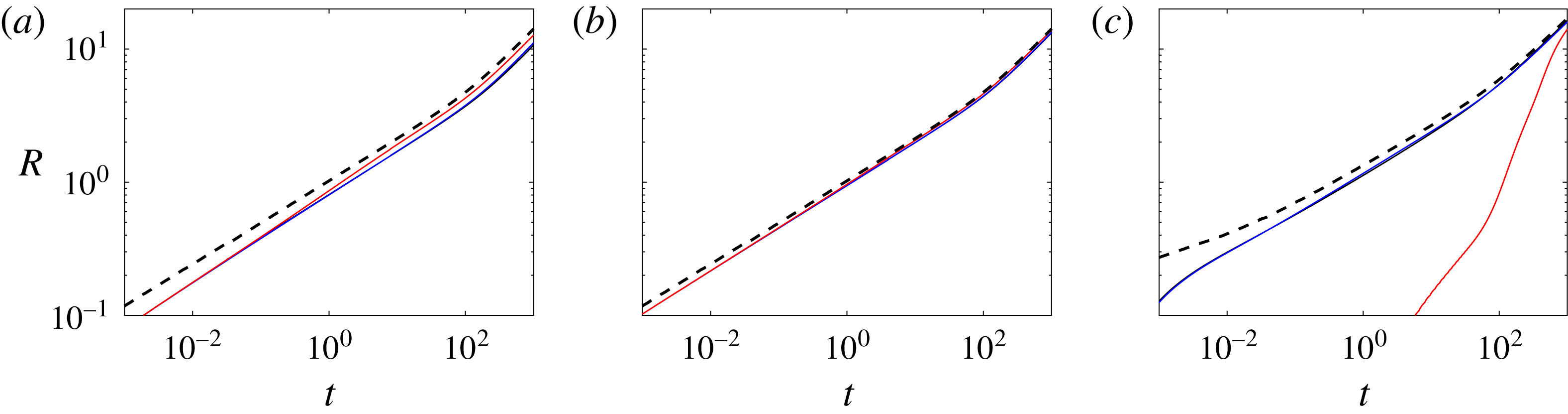
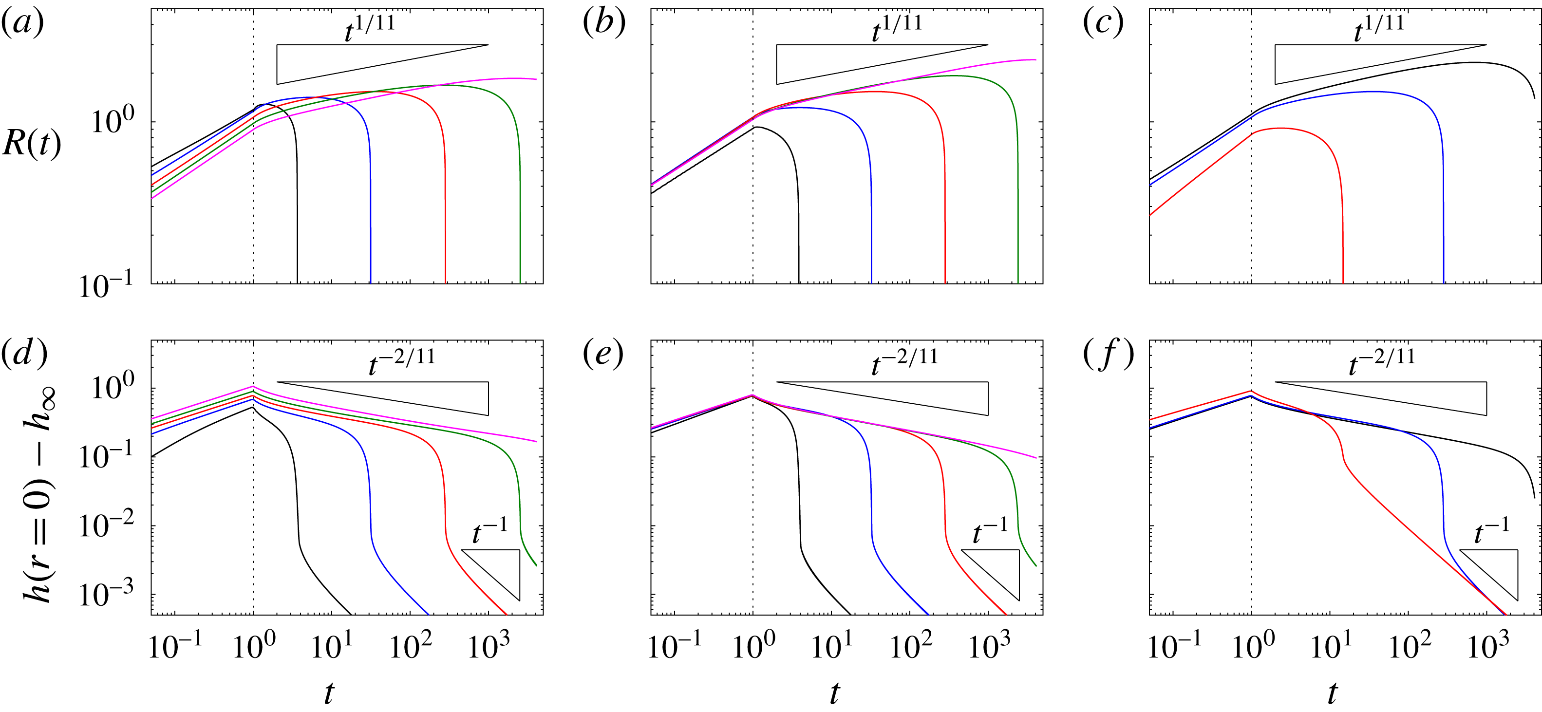
(red). The black dashed line shows the corresponding solution with a rigid till.
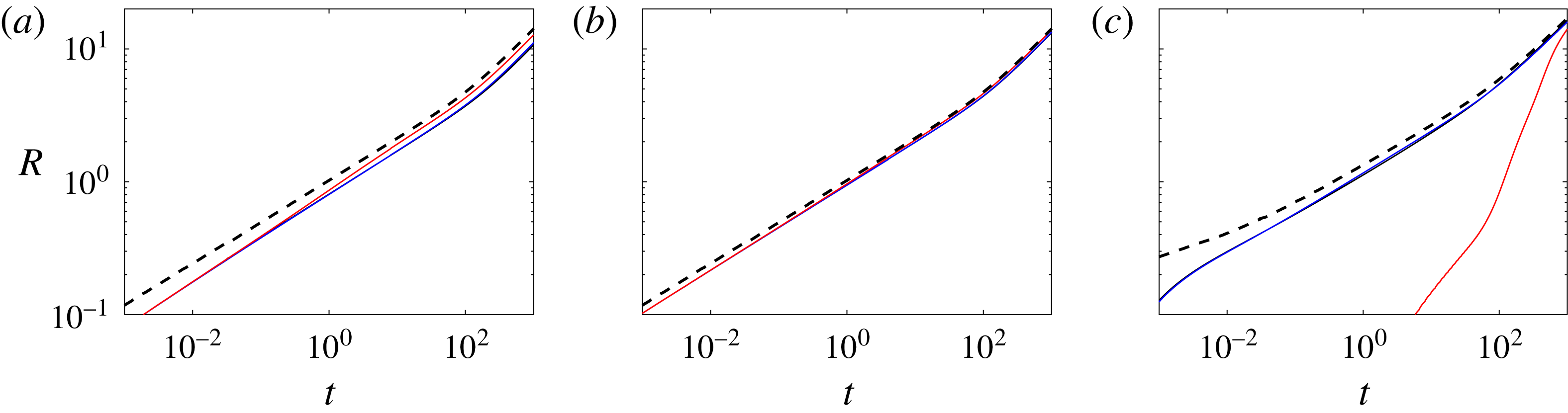
The simplest conclusion of this analysis is thus that the cavity spreads as though it were above a rigid medium, but with roughly
 $O(1)$
variations in the curvature
 $A$
. This conclusion is demonstrated by the solutions in figure 9, which show that the radius of the cavity for a variety of computations is relatively well approximated by the solution for a rigid till. Note that the cavity above a deformable till is always shorter and higher than that above a rigid till, because the rigid limit
 $A\rightarrow 1.58$
is a minimum of the curvature (see figure 8
d). Note also that figure 9(c) shows one calculation in which the cavity evolves quite differently: here the cavity only forms at all after a very long time (
 $t_{s}$
in (4.4) is very large), and the majority of the injected fluid has already spread through the till rather than forming a cavity.
Snapshots and data from computations with
 $Da=10^{-8}$
and
 $\tilde{M}=10^{4}$
(blue) and
 $\tilde{M}=10^{6}$
(red). (a,b) Snapshots of the uplift, focused on the nose, at (a)
 $t=2^{-3}$
and (b)
 $t=2^{5}$
. (c) The radius of the cavity
 $R(t)$
(thin solid lines) and extent of the deformation in the till
 $R_{\infty }(t)$
(thick solid lines). (d) The height of the uplift at the origin. The early-time bending scaling
 $t^{1/6}$
and diffusion scaling
 $t^{1/2}$
are also shown, together with the predictions of
 $R$
and
 $h$
from (3.6), for
 $\unicode[STIX]{x1D6E4}\ll 1$
and
 $f_{\infty }=\tilde{h}_{\infty }/(12Da)^{1/3}=-2.03$
, for which
 $A=3.46$
(dashed lines in (c) and (d)). The other parameters are
 $\tilde{Q}=1$
and
 $\tilde{h}_{\infty }=-0.01$
, and the green stars in (c,d) indicate the times of the snapshots in (a,b). Note that the kinks in
 $R_{\infty }$
correspond to oscillations in the uplift ahead of the cavity.

Two more detailed examples, which highlight the subtle differences in the solutions, are shown in figures 10 and 11. The figures show snapshots of both radius and height of the cavity, together with a measure of the extent
 $R_{\infty }$
of the deformation in the till, which we define to be the smallest radius such that
 $h(R_{\infty })$
is within
 $1\,\%$
of its far-field value
 $\tilde{h}_{\infty }$
.
Figure 10(a,b) shows snapshots at two different till stiffnesses for a low till permeability. Both solutions exhibit a low-
 $\unicode[STIX]{x1D6E4}$
bending wave at the nose initially (figure 10
a), but, over time, the signal of deformation begins to grow ahead of the nose for the solution with the larger stiffness (figure 10
b). This behaviour, which is indicative of the growth of
 $\unicode[STIX]{x1D6E4}$
over time, can also be observed in the data in figure 10(c):
 $R_{\infty }$
exhibits a transition to a diffusive scaling
 ${\sim}t^{1/2}$
while the cavity continues to spread like
 $t^{7/22}$
. Ultimately both
 $R$
and
 $R_{\infty }$
scale with
 $t^{1/2}$
, once gravity dominates the flow. Note that the higher-stiffness solution spreads slightly faster and has a slightly lower uplift than the lower-stiffness solution: this is a consequence of the higher value of
 $\unicode[STIX]{x1D6E4}$
here, which leads to a lower value of
 $A$
in (3.6). Note also that the lower-stiffness solution is well described by the theory with
 $\unicode[STIX]{x1D6E4}\ll 1$
until gravity plays a role.
Snapshots and data from computations with
 $Da=10^{-5}$
and
 $\tilde{M}=10^{4}$
(blue) and
 $\tilde{M}=10^{6}$
(red). (a,b) Snapshots of the uplift, focused on the nose, at (a)
 $t=2^{-3}$
and (b)
 $t=2^{5}$
. (c) The radius of the cavity
 $R(t)$
(thin solid lines) and extent of the deformation in the till
 $R_{\infty }(t)$
(thick solid lines). (d) The height of the uplift at the origin. The early-time bending scaling
 $t^{1/6}$
and diffusion scaling
 $t^{1/2}$
are also shown, as is the prediction of the height at early times from (4.1) (dotted line in d). Predictions of
 $R$
and
 $h$
from (3.6), for
 $\unicode[STIX]{x1D6E4}\ll 1$
and
 $f_{\infty }=\tilde{h}_{\infty }/(12Da)^{1/3}=-0.0203$
, for which
 $A=1.79$
, are also shown in (c) and (d) (dashed lines). The other parameters are
 $\tilde{Q}=1$
and
 $\tilde{h}_{\infty }=-0.01$
, and the green stars in (c,d) indicate the times of the snapshots in (a,b). Note again that the kinks in
 $R_{\infty }$
correspond to oscillations in the uplift ahead of the cavity.

Figure 11 shows the same data but for computations with a higher till permeability. Thus,
 $\unicode[STIX]{x1D6E4}$
is slightly larger and the snapshots (figure 11
a,b) show a clear evolution towards stiffness-dominated uplift ahead of the nose, much earlier than before. Despite this, the theoretical prediction for
 $\unicode[STIX]{x1D6E4}\ll 1$
still gives a good fit with the lower-stiffness computation (in which we estimate
 $\unicode[STIX]{x1D6E4}\approx 0.3$
initially, growing by roughly an order of magnitude over the course of the simulation). Note that, unlike in the previous figure, the cavity spreads more slowly here when the stiffness is larger. This is because the diffusive signal in the till spreads far ahead of the cavity, causing an increase in the flux
 $c$
and thus a larger curvature
 $A$
(as in figure 8
d).
4.5 Spread of the cavity for a fixed volume
Snapshots of the uplift
 $h(r,t)$
when
 $\tilde{Q}=1$
for
 $t<1$
and then
 $\tilde{Q}=0$
, to give a constant volume
 $\tilde{V}=1$
. Profiles are shown in each panel at times, from left to right,
 $t=1$
,
 $t=2^{2}$
,
 $t=2^{4}$
and
 $t=2^{6}$
. Lower panels show an enlarged version of the same data, to reveal the form of the uplift in the till; black lines show
 $z=0$
(long dashed) and
 $z=\tilde{h}_{\infty }$
(short dashed) for reference. (a) ‘High’ permeability (
 $Da=10^{-4}$
, blue) and ‘low’ permeability (
 $Da=10^{-8}$
, red), each with
 $\tilde{M}=10^{4}$
. (b) ‘High’ stiffness (
 $\tilde{M}=10^{6}$
, blue) and ‘low’ stiffness (
 $\tilde{M}=10^{2}$
, red), each with
 $Da=10^{-6}$
.

We end this section by considering the spread of a fixed volume over a deformable till. Given the conclusions in the previous subsection, if the injection flux is set to zero at time
 $t_{v}$
we expect the fluid-filled cavity to evolve like the solution for the rigid till (3.7), but with a curvature
 $A(c,\unicode[STIX]{x1D6E4})$
given by matching to the deformation in the till ahead.
Figure 12 shows snapshots over time of the spread of a constant volume over a deformable till, for different parameters. Unlike in the previous section, the figure suggests that the evolution of the flow is strongly dependent on the till permeability and stiffness, with the cavity rapidly draining away completely into the till if it is sufficiently permeable or stiff. This behaviour is corroborated by the results of a set of simulations in figure 13. The figure shows that, after the injection flux stops, the fluid initially spreads as it would over a rigid base, as described by (3.6). However, the radius of the cavity recedes relatively rapidly over some critical time, and the height drops away much faster than predicted. The time scale for collapse of the cavity appears to scale roughly with the inverse of
 $Da$
,
 $\tilde{M}$
and
 $\tilde{h}_{\infty }$
. This strong dependence on the parameters, in particular the stiffness
 $\tilde{M}$
, contrasts with the behaviour for a fixed flux, where the evolution of the cavity does not vary significantly across a wide range of parameters.
Data from numerical solutions when
 $\tilde{Q}=1$
for
 $t<1$
and then
 $\tilde{Q}=0$
, to give a constant volume
 $\tilde{V}=1$
. (a–c) The position
 $R(t)$
of the nose, and (d–f) the total height of the uplift
 $h-\tilde{h}_{\infty }$
at the origin. Different columns show solutions for different parameters: (a,d)
 $Da=(10^{-3},10^{-4},10^{-5},10^{-6},10^{-7})$
, (b,e)
 $\tilde{M}=(10^{6},\,10^{5},\,10^{4},10^{3},\,10^{2})$
and (c,f)
 $\tilde{h}_{\infty }=-(10^{-3},\,10^{-2},\,10^{-1})$
(in each case, black, blue, red, green, pink, respectively). Other parameters in each case are
 $Da=10^{-5}$
,
 $\tilde{M}=10^{4}$
and
 $\tilde{h}_{\infty }=-10^{-2}$
. Vertical dotted lines show the time at which the flux is set to zero. Black triangles show theoretical scalings.

The drainage of the cavity into the till here is a result of the leakage flux
 $q_{R}$
through the nose (4.10). When the cavity is being fed by a constant volume flux, the scaled flux
 $c$
is either constant (if the nose matches directly to
 $\tilde{h}_{\infty }$
ahead) or given by (4.20) (if the nose matches to a diffusive signal ahead). In either case, the magnitude of
 $q_{R}$
remains negligibly small relative to the constant injection flux, and
 $V^{\ast }\approx \tilde{Q}t$
remains a good approximation for the volume of fluid in the cavity in (3.2). However, once the injection flux stops, the volume lost by leakage may no longer be negligible relative to the now fixed volume
 $\tilde{V}$
in the cavity. In fact, since the spread of the cavity becomes much slower after injection,
 ${\dot{R}}$
becomes much smaller and
 $\unicode[STIX]{x1D6E4}$
grows significantly. Diffusion of pressure in the till thus rapidly overtakes the cavity once injection stops, which indicates that the leakage flux rapidly evolves to be given by (4.19):
 $$\begin{eqnarray}q_{R}\sim \frac{4\unicode[STIX]{x03C0}Da\,\tilde{M}\,|\tilde{h}_{\infty }|}{\log (Da\,\tilde{M}\,t)}.\end{eqnarray}$$
A balance of the available volume
 $\tilde{V}$
in the cavity with the integrated volume lost over time by leakage into the till ahead (4.21) suggests that the cavity will have collapsed after a time scale
 $$\begin{eqnarray}t\sim \frac{\tilde{V}}{Da\tilde{M}|\tilde{h}_{\infty }|},\end{eqnarray}$$
(ignoring logarithmic corrections and
 $O(1)$
constants). That is, the time to drain the cavity scales inversely with
 $Da$
,
 $\tilde{M}$
and
 $\tilde{h}_{\infty }$
, in agreement with the results in figure 13.
Once the cavity has drained, the remaining relaxation of the till is governed by classical poroelastic diffusion (4.6). The radial extent of the pressure signal spreads over a scale
 $r\sim (Da\tilde{M}t)^{1/2}$
and the height at the origin drops like
 $t^{-1}$
(seefigure 13
d–f).
In summary, when the rate of advance of the cavity is rapid, as it is for a constant volumetric influx or initially for the spreading of a constant volume, the qualitative spread of the cavity is unaffected by the properties of the till, although they have some signature in the uplift ahead of the cavity. However, as the cavity slows and poroelastic diffusion outpaces the advance of the cavity, a significant fluid volume leaks into the far field, resulting in a relatively rapid cavity collapse. Given the weak dependence on till properties during the initial propagation, it is therefore worth noting that the major observable feature that might constrain the properties of the subglacial till would be the scale over which the cavity collapses.
5 Turbulent flow in the cavity
The drainage of supraglacial lakes is sufficiently rapid that in many cases the initial flow is likely to be turbulent over a significant fraction of the cavity, as modelled previously by Tsai & Rice (Reference Tsai and Rice2010) in a limit in which the glacier was frozen to the bedrock. In this final section, we briefly consider the effect of turbulent, rather than laminar, flow in the cavity. In particular, and unlike in previous studies, we focus here on determining when turbulence, rather than laminar peeling at the front, determines the rate of propagation.
Since the height of the cavity, and thus the effective local Reynolds number of the flow, always decreases to zero where the glacier touches the till, there must still be a region of laminar flow sufficiently close to the nose, irrespective of how vigorously the fluid flows through the bulk of the cavity. Thus, following previous work for flow in fractures (Dontsov Reference Dontsov2016), we introduce a very simple phenomenological relationship between the driving radial pressure gradient in the cavity and the mean flow
 $U$
, which is parameterised by an effective local Reynolds number
 $Re$
for the flow. This relationship reduces to the laminar and turbulent limits,
 $\unicode[STIX]{x2202}p/\unicode[STIX]{x2202}r\sim U$
as
 $Re\rightarrow 0$
and
 $\unicode[STIX]{x2202}p/\unicode[STIX]{x2202}r\sim U^{2}$
as
 $Re\rightarrow \infty$
. To avoid overly muddying the analysis, we choose an extremely simple relationship: the aim here is not so much to provide a detailed empirical description for flow in the cavity at arbitrary Reynolds number, but rather to gain qualitative insight into the relative importance of turbulence in the interior, as opposed to viscous peeling at the front, in determining the propagation of the cavity.
5.1 Simple model for hybrid turbulent–laminar flow
Following standard formulations for flow in channels and pipes, we introduce a Darcy–Weisbach friction factor
 $f_{D}(Re)$
for flow in the cavity, which relates the driving pressure gradient
 $\unicode[STIX]{x2202}p/\unicode[STIX]{x2202}r$
to the mean radial flow
 $U$
via
 $$\begin{eqnarray}-\frac{\unicode[STIX]{x2202}p}{\unicode[STIX]{x2202}r}=f_{D}(Re)\frac{\unicode[STIX]{x1D70C}U^{2}}{4h},\end{eqnarray}$$
in terms of the (dimensional) height of the cavity
 $h$
, density of fluid
 $\unicode[STIX]{x1D70C}$
, and Reynolds number
 $$\begin{eqnarray}Re\equiv \frac{\unicode[STIX]{x1D70C}Uh}{\unicode[STIX]{x1D707}}.\end{eqnarray}$$
For laminar flow, this relationship has already been determined in (2.7a
) (with
 $U\equiv q/(rh)$
, and considering only the contribution from the cavity in that expression), and gives
 $$\begin{eqnarray}-\frac{\unicode[STIX]{x2202}p}{\unicode[STIX]{x2202}r}=\frac{12\unicode[STIX]{x1D707}}{h^{2}}U,\quad \;\Longrightarrow \;\quad f_{D}(Re\rightarrow 0)\rightarrow \frac{48}{Re}.\end{eqnarray}$$
For turbulent flow with
 $Re\gg 1$
, we instead make a phenomenological argument that the mean turbulent flow
 $U$
is bounded by viscous shear layers of width
 $\unicode[STIX]{x1D6FF}\ll h$
against the top (ice) and bottom (till) surfaces of the cavity. We can estimate the scale of these layers by assuming the local boundary-layer Reynolds number is held at some critical value
 $Re_{c}\sim O(10^{3})$
(this parameter also incorporates the effects of wall roughness and can vary significantly; see e.g. Dontsov Reference Dontsov2016) such that
 $$\begin{eqnarray}\frac{\unicode[STIX]{x1D70C}U\unicode[STIX]{x1D6FF}}{\unicode[STIX]{x1D707}}\simeq Re_{c}.\end{eqnarray}$$
A balance of the pressure gradient with the viscous stresses from the two boundaries thus gives
 $$\begin{eqnarray}-\frac{\unicode[STIX]{x2202}p}{\unicode[STIX]{x2202}r}h\simeq 2\unicode[STIX]{x1D707}\frac{U}{\unicode[STIX]{x1D6FF}}\simeq 2\unicode[STIX]{x1D707}U\frac{\unicode[STIX]{x1D70C}U}{\unicode[STIX]{x1D707}Re_{c}},\end{eqnarray}$$
and hence
 $$\begin{eqnarray}f_{D}(Re\gg 1)\simeq \frac{8}{Re_{c}}.\end{eqnarray}$$
Perhaps the simplest possible patch of the two limits in (5.3) and (5.6) is an additive composite,
 $$\begin{eqnarray}f_{D}(Re)\simeq \frac{8}{Re_{c}}+\frac{48}{Re},\end{eqnarray}$$
for which (5.1) reduces to
 $$\begin{eqnarray}-\frac{4\unicode[STIX]{x1D70C}h^{3}}{\unicode[STIX]{x1D707}^{2}}\frac{\unicode[STIX]{x2202}p}{\unicode[STIX]{x2202}r}=Re^{2}\left(\frac{8}{Re_{c}}+\frac{48}{Re}\right).\end{eqnarray}$$
More usefully, we can invert this relationship and combine with (5.2) to give
 $$\begin{eqnarray}Uh=\text{sgn}(G)\frac{3\unicode[STIX]{x1D707}Re_{c}}{\unicode[STIX]{x1D70C}}\left(\sqrt{1+\left|\frac{G}{72Re_{c}}\right|}-1\right),\end{eqnarray}$$
where
 $\text{sgn}(x)$
signifies the sign of
 $x$
, and
 $$\begin{eqnarray}G(h)=-\frac{4\unicode[STIX]{x1D70C}h^{3}}{\unicode[STIX]{x1D707}^{2}}\frac{\unicode[STIX]{x2202}p}{\unicode[STIX]{x2202}r}.\end{eqnarray}$$
We note that other empirical turbulence relationships incorporating wall roughness can be readily included in the analysis (see appendix C), but that this does not significantly alter either the physical model or the spreading behaviour.
Given (5.9), we can simply replace the relevant flux term in (2.7a
), and combine with mass conservation (2.8) to give a new evolution equation for the uplift of the glacier for
 $h>0$
. Such an operation yields
 $$\begin{eqnarray}\frac{\unicode[STIX]{x2202}h}{\unicode[STIX]{x2202}t}+\frac{1}{r}\frac{\unicode[STIX]{x2202}}{\unicode[STIX]{x2202}r}\left(\frac{rkb_{0}}{\unicode[STIX]{x1D707}}\frac{\unicode[STIX]{x2202}p}{\unicode[STIX]{x2202}r}\right)+\frac{1}{r}\frac{\unicode[STIX]{x2202}}{\unicode[STIX]{x2202}r}(r\,Uh)=0,\end{eqnarray}$$
which, when combined with an expression for the pressure gradient from (2.5), replaces (2.9a
) as the governing equation for
 $h>0$
. In terms of dimensionless quantities, scaling as in § 2.4, (5.11) reduces to
 $$\begin{eqnarray}\frac{\unicode[STIX]{x2202}h}{\unicode[STIX]{x2202}t}+\frac{1}{r}\frac{\unicode[STIX]{x2202}}{\unicode[STIX]{x2202}r}\left(r\,Da\frac{\unicode[STIX]{x2202}p}{\unicode[STIX]{x2202}r}\right)+\text{sgn}\left(\frac{\unicode[STIX]{x2202}p}{\unicode[STIX]{x2202}r}\right)\frac{1}{r}\frac{\unicode[STIX]{x2202}}{\unicode[STIX]{x2202}r}\left[\frac{r}{6{\mathcal{R}}_{e}}\left(-1+\sqrt{1+{\mathcal{R}}_{e}h^{3}\left|\frac{\unicode[STIX]{x2202}p}{\unicode[STIX]{x2202}r}\right|}\right)\right]=0,\end{eqnarray}$$
for
 $h>0$
, where
 $\unicode[STIX]{x2202}p/\unicode[STIX]{x2202}r=-(\unicode[STIX]{x2202}/\unicode[STIX]{x2202}r)(h+\unicode[STIX]{x1D6FB}^{4}h)$
is the driving pressure gradient and the parameter
 $$\begin{eqnarray}{\mathcal{R}}_{e}\equiv \frac{1}{18Re_{c}}\frac{b_{0}^{4}}{\unicode[STIX]{x1D707}^{2}}\left(\frac{\unicode[STIX]{x1D70C}^{9}g^{5}}{B}\right)^{1/4}=\frac{2}{3Re_{c}}\left[\frac{b_{0}^{2}}{12\unicode[STIX]{x1D707}}\frac{\unicode[STIX]{x1D70C}gb_{0}}{L}\right]\frac{\unicode[STIX]{x1D70C}b_{0}}{\unicode[STIX]{x1D707}},\end{eqnarray}$$
is a scaled effective Reynolds number, based on the depth of the till and an elasto-gravity velocity scale written in terms of the bending length
 $L$
in (2.12). The original viscous model (2.13a
) is recovered in the limit
 ${\mathcal{R}}_{e}\rightarrow 0$
.
5.2 Implications of the hybrid model
For simplicity we consider flow above a rigid till. In the vicinity of the nose, a local travelling-wave solution of (5.12) satisfies
 $$\begin{eqnarray}-{\dot{R}}h=Dah^{(v)}-\frac{1}{6{\mathcal{R}}_{e}}\left(-1+\sqrt{1-{\mathcal{R}}_{e}h^{3}h^{(v)}}\right),\end{eqnarray}$$
having integrated once, and under the assumption that the pressure gradient is positive throughout the region. If the last term inside the square root is small inside the nose region, then (5.14) reduces to the laminar balance (3.3). Given the height and length scales of the nose region, this constraint reduces to
 $$\begin{eqnarray}\frac{{\mathcal{R}}_{e}(12Da)^{4/3}}{(Da/{\dot{R}})}<O(1),\quad \text{or}\quad {\mathcal{R}}_{e}\lesssim \frac{1}{12{\dot{R}}(12Da)^{1/3}}.\end{eqnarray}$$
In this limit, the pressure drop is still dominated by peeling at the nose, where the flow is laminar. The turbulent cavity thus remains at a uniform pressure to leading order and spreads exactly as before, controlled by laminar peeling at the front.
If, however, (5.15) does not hold, then the nose region is no longer fully laminar. In this situation, we find a qualitative change in the flow: the nose can no longer approach the interior cavity as a quadratic, which suggests that the construction of a constant-pressure cavity and a peeling nose must break down. Indeed, as briefly outlined in appendix B, once turbulence enters the peeling region, the height of the cavity approaches the nose like
 $(R-r)^{5/2}$
and the pressure is no longer uniform to leading order across the cavity. In this limit, the dominant contribution in (5.12) is from turbulent flow in the cavity. Provided that bending stresses, rather than gravity, dominate the pressure gradient (i.e.
 $R\lesssim 1$
), (5.12) reduces to
 $$\begin{eqnarray}\frac{\unicode[STIX]{x2202}h}{\unicode[STIX]{x2202}t}\approx \frac{1}{6\sqrt{{\mathcal{R}}_{e}}r}\frac{\unicode[STIX]{x2202}}{\unicode[STIX]{x2202}r}\left[r\sqrt[\ast ]{h^{3}\frac{\unicode[STIX]{x2202}}{\unicode[STIX]{x2202}r}\unicode[STIX]{x1D6FB}^{4}h}\right],\end{eqnarray}$$
where
 $\sqrt[\ast ]{x}=\text{sgn}(x)\sqrt{|x|}$
is a sign-preserving square root. For a constant injection flux, (5.16), together with (2.16), has a similarity solution which satisfies
 $$\begin{eqnarray}\frac{6}{11}\left(3f-4\unicode[STIX]{x1D702}\frac{\unicode[STIX]{x2202}f}{\unicode[STIX]{x2202}\unicode[STIX]{x1D702}}\right)=\frac{1}{\unicode[STIX]{x1D702}}\frac{\unicode[STIX]{x2202}}{\unicode[STIX]{x2202}\unicode[STIX]{x1D702}}\left[\unicode[STIX]{x1D702}\sqrt[\ast ]{f^{3}\frac{\unicode[STIX]{x2202}}{\unicode[STIX]{x2202}\unicode[STIX]{x1D702}}\left(\frac{1}{\unicode[STIX]{x1D702}}\frac{\unicode[STIX]{x2202}}{\unicode[STIX]{x2202}\unicode[STIX]{x1D702}}\unicode[STIX]{x1D702}\frac{\unicode[STIX]{x2202}}{\unicode[STIX]{x2202}\unicode[STIX]{x1D702}}\right)^{2}f}\right];\quad 2\unicode[STIX]{x03C0}\int _{0}^{\unicode[STIX]{x1D702}_{N}}f\unicode[STIX]{x1D702}\,\text{d}\unicode[STIX]{x1D702}=1,\end{eqnarray}$$
where
 $$\begin{eqnarray}\unicode[STIX]{x1D702}=r\left(\frac{\tilde{Q}^{2}}{{\mathcal{R}}_{e}}\right)^{-1/11}t^{-4/11},\quad h=\left(\tilde{Q}^{7}{\mathcal{R}}_{e}^{2}\right)^{1/11}t^{3/11}f(\unicode[STIX]{x1D702}),\end{eqnarray}$$
and
 $\unicode[STIX]{x1D702}_{N}$
is an eigenvalue which determines the location of the nose. The boundary conditions are
 $f^{\prime }(0)=f^{\prime \prime \prime }(0)=0$
and
 $f\sim (\unicode[STIX]{x1D702}_{N}-\unicode[STIX]{x1D702})^{5/2}$
as
 $\unicode[STIX]{x1D702}\rightarrow \unicode[STIX]{x1D702}_{N}$
(see appendix B), together with an integral constraint for the total volume. Numerical solution of (5.17) gives
 $\unicode[STIX]{x1D702}_{N}=1.308$
or
 $R(t)=1.308(\tilde{Q}^{2}/{\mathcal{R}}_{e})^{1/11}t^{4/11}$
.
Numerical solutions of the hybrid turbulent–laminar model for
 ${\mathcal{R}}_{e}=1$
(black),
 ${\mathcal{R}}_{e}=10$
(blue),
 ${\mathcal{R}}_{e}=100$
(red) and
 ${\mathcal{R}}_{e}=10^{3}$
(green). All computations have a rigid till with
 $Da=10^{-10}$
and a fixed injection flux
 $\tilde{Q}=1$
. (a) Snapshots of the height of the cavity
 $h$
at
 $t=0.5$
, together with the constant-pressure cavity prediction (black dotted) and the turbulent similarity solution of (5.16) (green dashed, for
 ${\mathcal{R}}_{e}=10^{3}$
). (b) The cavity radius
 $R(t)$
, for the same computations, and (c) the scaled cavity radius
 $R/t^{7/22}$
. Again, the prediction for a laminar nose (black dotted, from (3.6)) and that for a turbulent nose (green dashed, for
 ${\mathcal{R}}_{e}=10^{3}$
from (5.18)) are shown. Solutions evolve from the latter toward the former. At later times, gravity dominates and the spreading becomes faster.

Figure 14 shows numerical solutions of the full hybrid problem (5.12) for different values of
 ${\mathcal{R}}_{e}$
, which demonstrate the transition between laminar and turbulent flow at the nose. The clearest qualitative effect of a higher value of
 ${\mathcal{R}}_{e}$
is that the cavity is shorter and higher (figure 14
a), which is a consequence of the increased dissipation in the flow. The evolution of the cavity, however, is remarkably similar between the laminar and turbulent limits: the evolution of
 $R(t)$
described by (3.6) and (5.18) differs only by a factor of
 $(t^{3}/\tilde{Q}^{3}{\mathcal{R}}_{e}^{6}Da)^{1/66}$
, which is reflected by the nearness of the curves in figure 14(b). These curves also show that solutions gradually evolve from a fully turbulent cavity towards a constant-pressure cavity with a laminar nose over time, as the flow slows down. This behaviour is particularly clear if the results are rescaled (figure 14
c). Given the scalings in (5.18) and the laminar nose constraint (5.15), the time over which the flow evolves to the laminar peeling solution is
 $$\begin{eqnarray}t\sim {\mathcal{R}}_{e}^{10/7}\tilde{Q}^{2/7}Da^{11/21},\end{eqnarray}$$
over which time the cavity has reached a size
 $$\begin{eqnarray}R\sim {\mathcal{R}}_{e}^{3/7}\tilde{Q}^{2/7}Da^{4/21}.\end{eqnarray}$$
Note that after this time, the evolution of the cavity is again governed by peeling in the laminar nose region, and the pressure in the cavity is roughly uniform. The flow may still be turbulent in the interior of the cavity, but this has no effect to leading order: the pressure drop associated with any flow in the cavity, turbulent or laminar, is small relative to that required to peel the glacier off the till at the nose.
Once the injection stops, the remaining volume
 $\tilde{V}$
of fluid again continues to spread. In the fully turbulent limit governed by (5.16), the similarity scaling now indicates that
 $R(t)\sim t^{2/11}$
. The rate of advance
 ${\dot{R}}$
is therefore smaller, and so the peeling region will become fully laminar even more quickly, given the constraint (5.15). Thus, the flow will rapidly evolve to a situation in which the previous results for laminar flow again apply. In particular, for flow over a deformable till, the spreading current will again ‘leak’ fluid through the nose into the till ahead, as described in § 4.5, and the cavity will again collapse into the till over the same time scale (4.22). In fact, even if the flow remains fully turbulent at the nose, matching between the turbulent nose and poroelastic diffusion in the till indicates that leakage will occur over the same time scale. Figure 15 shows full solutions of the spread of a constant volume for different
 ${\mathcal{R}}_{e}$
, which demonstrates this behaviour.
Numerical solutions of the hybrid turbulent–laminar model when the injection flux
 $\tilde{Q}=1$
is set to zero at time
 $t_{v}=1$
, and the till is deformable with
 $\tilde{M}=10^{5}$
and
 $\tilde{h}_{\infty }=-0.01$
. Different lines have
 ${\mathcal{R}}_{e}=10$
(blue),
 ${\mathcal{R}}_{e}=10^{3}$
(red) and
 ${\mathcal{R}}_{e}=0$
(i.e. fully laminar; black dashed). (a)
 $Da=10^{-5}$
and (b)
 $Da=10^{-7}$
.

6 Implications
6.1 Geophysical implications
The previous sections outline the various physical processes that may give rise to the observed, transient measurements of uplift and enhanced basal sliding associated with the rapid drainage of supraglacial lakes. Here we briefly discuss some of the implications of our model and discuss how future interpretation of the geophysical data could further constrain the properties of the subglacial till, leaving a detailed comparison with geophysical data for future work.
The drainage, and rapid propagation, of supraglacial melt water has been measured using a dense GPS network in Greenland (Das et al. Reference Das, Joughin, Behn, Howat, King, Lizarralde and Bhatia2008; Stevens et al. Reference Stevens, Behn, McGuire, Das, Joughin, Herring, Shean and King2015). These data sets measure the relative motion of points surrounding the supraglacial lakes throughout the melt season, and have been processed to infer spatial patterns of uplift and enhanced sliding rates of glacial ice associated with the rapid drainage of a reasonably well-constrained volume of melt water. Analysis of the resulting data may enable inference of the properties of the subglacial till and a more detailed examination, on relatively short time scales, of the influence of melt water (or pore pressure) on the coupling between ice velocity and the subglacial environment. To aid in the comparison between predictions of our model and the geophysical observations, table 1 shows a compilation of the non-dimensional and dimensional model results.
Summary of non-dimensional and dimensional model results, showing the time taken for the cavity to first appear, and predictions for the radius and height of the cavity for both turbulent and laminar flow in the cavity. For the laminar case, the predictions are shown both for a rigid and a deformable till. In the latter case, we have shown the results for a fairly stiff till in which the pressure signal does not spread ahead of the travelling-wave region (i.e.
 $\unicode[STIX]{x1D6E4}\gg 1$
;
 $R(t)\gg X(t)$
); in general, the parameter
 $A$
varies over time as discussed in § 4.4. Dimensional variables are all defined in § 2, and
 $h_{\infty }=(p_{\infty }-\unicode[STIX]{x1D70C}_{i}gd)b_{0}/M$
, as in (2.3).
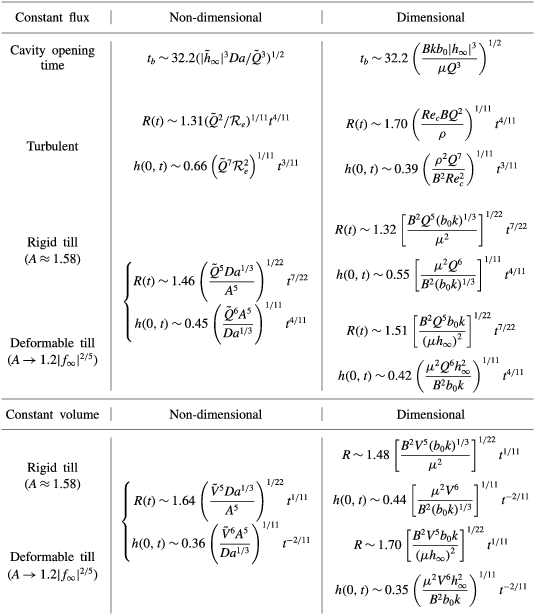
To focus the analysis, we take the results of the 2011 drainage event described in Stevens et al. (Reference Stevens, Behn, McGuire, Das, Joughin, Herring, Shean and King2015) as a specific example. In § 2.5, an estimate of the natural flexural length scale of the glacial ice of 1.4–2.5 km was shown to be comparable to the flexural signal seen in the GPS observations. In addition, the geophysical observations indicate that a lake volume
 $V=0.0077\pm 0.001$
km
 $^{3}$
drained in
 ${\sim}3$
h, from which a mean flux of
 $Q\simeq 710~\text{m}^{3}~\text{s}^{-1}$
can be inferred. Given these predictions, the transition time for turbulent-to-laminar control calculated from (5.19) is
 $\simeq 4\,000$
h, which is far in excess of the
 ${\sim}3$
h initial rapid flux of lake water, and suggests that the initial drainage (over the first 3 h) was controlled by turbulent dissipation. An estimate from the turbulent model in § 5 suggests that the cavity would have grown to a size
 $R\simeq 5.0{-}6.3$
km over these three hours, with a central uplift of
 $h(0,t)\simeq 0.2{-}0.35$
m; both of these predictions are roughly consistent with the GPS observations, which suggest a maximum central uplift of
 ${\sim}0.6~\text{m}$
(Stevens et al.
Reference Stevens, Behn, McGuire, Das, Joughin, Herring, Shean and King2015). We note that, once lake drainage had ceased and the water volume within the cavity was constant, a transition to laminar flow is likely to have occurred rapidly (as discussed at the end of § 5.2), such that subsequent propagation of the cavity would have been controlled by laminar peeling at its nose.
The present analysis is also suggestive of both the initiation of the hydrofracturing event, and the eventual subsidence of the observed uplift. A key conclusion of Stevens et al. (Reference Stevens, Behn, McGuire, Das, Joughin, Herring, Shean and King2015) is that rapid drainage of supraglacial lakes is preceded by a transient uplift, driven by the slow percolation of melt water to the base of the ice sheet, which causes enhanced basal sliding. This enhanced basal sliding naturally produces a localised divergence in the ice velocity, leading to the horizontal fractures, or crevasses, which provide a fast route for water to reach the bed and are characteristic of rapid supraglacial lake drainage events. While we make no attempt here to model the transport of melt water to the base of the glacier (see e.g. Rice et al.
Reference Rice, Tsai, Fernandes and Platt2015), our model suggests that, in the presence of a poroelastic subglacial till, an initial, small, melt water flux to the base may locally increase the pore pressure within the till. After a characteristic time, summarised in table 1, this melt water flux is sufficient to lift the base of the ice sheet off the till, a point certainly concomitant with an enhancement of basal sliding. Subsequent initiation of crevassing would cause a rapid increase in the flux of melt water to the base, triggering the turbulent expansion of the subglacial cavity. During this transient activity, and shortly after the end of the drainage event, the geophysical data (see e.g. the supplementary movies of Stevens et al.
Reference Stevens, Behn, McGuire, Das, Joughin, Herring, Shean and King2015) suggest a flexural signal in the uplift of the ice at the extremities of the expanding cavity, with a vertical amplitude of roughly
 ${\sim}0.1~\text{m}$
.
While it is not possible to constrain all the properties of the subglacial till without a more detailed analysis, we can demonstrate that our model predictions, together with plausible parameter estimates, are consistent with this observation. For example, using a subglacial till thickness
 $b_{0}\simeq 1$
m, permeability
 $k\simeq 10^{-12}~\text{m}^{2}$
, and stiffness
 $M\simeq 10^{8}~\text{Pa}$
, which are consistent with the geophysical data of Stevens et al. (Reference Stevens, Behn, McGuire, Das, Joughin, Herring, Shean and King2015), the results of the model in § 4.3 (after redimensionalisation) suggest that the vertical flexural amplitude would decrease over time from a ‘soft’-till limit
 $|h_{\infty }|\simeq \unicode[STIX]{x1D70C}_{i}gdb_{0}M^{-1}\simeq 0.1~\text{m}$
, which is consistent with the data, towards a ‘stiff’-till limit
 $b_{0}Da^{1/3}=(b_{0}k)^{1/3}\simeq 10^{-4}~\text{m}$
. These same values suggest that for an uplift time of 8 h, corresponding to the duration of the measured precursor (Stevens et al.
Reference Stevens, Behn, McGuire, Das, Joughin, Herring, Shean and King2015), the mean magnitude of the precursor flux would be
 $Q\simeq 0.3~\text{m}^{3}~\text{s}^{-1}$
(using table 1). While these results are suggestive, it is perhaps most pertinent to conclude that the qualitative similarity between the structure of the geophysical observations and the results of the model indicates that the properties of a poroelastic, subglacial till may indeed determine both the initial and the eventual long-term response of ice sheets to the drainage of supraglacial lakes. A more detailed analysis may provide more quantitative estimates of the controlling properties of this subglacial till; we leave such an analysis for future investigation.
6.2 Qualitative comparison with previous models
The modelling framework here is most similar to that used by Tsai & Rice (Reference Tsai and Rice2010) and Adhikari & Tsai (Reference Adhikari and Tsai2015). Both of these studies employed a fully turbulent parameterisation for flow in the cavity, with no porous till, and used a ‘deep’ approximation of the ice as an elastic half space. Tsai & Rice (Reference Tsai and Rice2010) used a model of fracturing at the tip, which does not allow for any leakage or spread of pressure ahead of the cavity. Adhikari & Tsai (Reference Adhikari and Tsai2015) instead coupled the spread of the cavity to a pre-existing subglacial hydrological network, parameterised by thin fluid layer, which allows for propagation of a flexural signal ahead of the cavity. Our investigation contains two significant differences: we account for a deformable porous till below the glacier; and we consider both a laminar and a hybrid turbulent–laminar model for the flow within the cavity. We also employ the opposite approximation of a shallow bending beam for the ice, rather than an elastic half-space (see § 2.2).
If the flow in the cavity is strongly turbulent, the predictions of this work broadly match those of Tsai & Rice (Reference Tsai and Rice2010) and Adhikari & Tsai (Reference Adhikari and Tsai2015): poroelastic deformation in the till plays a negligible role in its spread. It does, however, affect the diffusion of pressure into the wider hydrological system ahead of the cavity, and thus the observable flexural signals in the ice. At later times as the cavity slows, however, laminar control is reasserted and the dynamics changes. A hybrid turbulent–laminar model is crucial for capturing this transition in the physical control of the spreading cavity from turbulent dissipation to laminar peeling and suction through the till at the nose as the cavity spreads; a fully turbulent model, as employed in previous work, would enforce a turbulent parameterisation even in regions where the gap width becomes arbitrarily narrow. Poroelastic deformation in the till also controls the leakage from and eventual collapse of the cavity; this raises the possibility of inferring properties of the subglacial hydrology from measurements of the eventual cavity collapse. Finally, poroelasticity of the till may play a key role in the initial precursor behaviour of slow leakage to the base, local lubrication of the ice sheet and diverging ice velocity, as discussed in the preceding subsection.
7 Conclusions
In this paper, we have developed and analysed a theoretical model of the spread of fluid at the base of an elastic sheet that is resting on a shallow, saturated, poroelastic bed. This model provides a framework in which to interpret observations of the drainage of supraglacial lakes in Greenland made by Das et al. (Reference Das, Joughin, Behn, Howat, King, Lizarralde and Bhatia2008), Stevens et al. (Reference Stevens, Behn, McGuire, Das, Joughin, Herring, Shean and King2015) and others. The model consists of a simplified description of the elastic flexure of glacial ice, using Euler–Bernoulli beam theory, coupled with the shallow flow of water within an expanding subglacial cavity and poroelastic till.
In § 3, we showed that the spreading of a laminar cavity above a rigid till is controlled by peeling at the nose of the cavity. Suction of pore fluid from the porous till allows the cavity to propagate, but the dependence of the spreading rate on the properties of the till is essentially negligible. We then extended this analysis to a deformable till in § 4. For laminar injection with a fixed flux, propagation can be broadly split into two regimes: first, in which variations in pore pressure associated with bending at the front are confined to a travelling wave during relatively rapid propagation; and second, in which diffusion of pore pressure through the till spreads faster than the spreading cavity. Each regime has different signatures in the pressure distribution ahead of the till, but the qualitative impact on the spreading of the cavity is both subtle and relatively weak. Again, the properties of the till have minimal impact on the spread of the cavity, although they do affect the coupling of the cavity to the till ahead. In contrast, for the spread of a fixed volume of fluid, the till properties play the dominant role in controlling the spread of the cavity, via the leakage flux.
In § 5, we used a simple hybrid parameterisation of turbulent–laminar flow to investigate the situation when the flow in the cavity is highly turbulent, as is likely to be the case for rapid supraglacial lake drainage (cf. Tsai & Rice Reference Tsai and Rice2010). In this limit, the cavity spreads self-similarly and is independent of the properties of the till (see the dimensional results quoted in table 1): turbulent dissipation within the cavity results in a large-scale radial pressure gradient across the cavity. However, as the radius of the cavity increases and the rate of expansion decreases, the flow becomes laminar in the nose: the pressure drop instead becomes dominated by peeling and suction from the till at the nose, and the cavity spreads as in the laminar cases discussed above. Note that flow in the majority of the cavity may still be turbulent in this limit provided the dominant pressure drop comes from laminar suction at the nose.
Finally, in § 6 we briefly compared our results with geophysical data, and found a qualitative reproduction of various key observations. This agreement suggests that, particularly during the melt season when supraglacial lakes are observed to drain, it is turbulent dissipation and flow through a poroelastic till which determine the subglacial extent of melt water propagation and hence lubrication. The properties of the till are unlikely to play a role in the rapid spread of the cavity, but will affect diffusion of pressure and leakage of water into the wider subglacial hydrological system, the long-term collapse of the cavity and the precursor and initiation stages of drainage. It is to be hoped that a more detailed comparison between model results and geophysical data might therefore yield further insights into the local lubrication conditions at the base of the Greenland ice sheet, and thus help to explain the observed ice velocity associated with lake drainage events.
Acknowledgements
The authors would like to acknowledge the helpful comments on many aspects of this work by G. G. Peng. The research of J.A.N. is partly supported by a Royal Society University Research Fellowship.
Appendix A. The slip velocity at the nose
We have assumed that the slip velocity
 $u_{b}$
in (2.6b
) is negligible in this paper; if it were included, it would give an additional contribution to the flux of order
 $hu_{b}\unicode[STIX]{x2202}h/\unicode[STIX]{x2202}r$
in (2.13a
). The no-slip condition on the boundary between the fluid and the saturated medium suggests that
 $u_{b}=O(Da)$
, while a more detailed balance gives a correction to this on the scale of the pore size,
 $O(Da^{1/2})$
(Le Bars & Worster Reference Le Bars and Worster2006). Given
 $Da\ll 1$
, the contribution from this flux is certainly negligible over the majority of the cavity, but could, in principle, play a role in the nose region near
 $r=R$
, where the flux through till and cavity become comparable. In that region,
 $h^{3}\sim Da$
, and so the extra contribution to the flux from the slip velocity is
 $O(Da^{4/3})$
. The other contributions to the flux in this region are
 $O(Da)$
, and so the slip velocity is also negligible in the nose region.
Appendix B. Behaviour at the nose in the laminar and turbulent limits
After suitable rescaling, steady solutions in a frame moving with the nose satisfy
 $$\begin{eqnarray}-f=f^{(v)}+f^{3}f^{(v)},\end{eqnarray}$$
if the flow is laminar, or
 $$\begin{eqnarray}-f=f^{(v)}-\sqrt{-f^{3}f^{(v)}},\end{eqnarray}$$
if the flow is fully turbulent. The former equation gives
 $f^{(\text{v})}\sim 1/f^{2}$
in the far field, which might suggest an approach to the nose of
 $f\sim \unicode[STIX]{x1D6FD}(R-r)^{5/3}$
for some
 $\unicode[STIX]{x1D6FD}>0$
. This solution is inconsistent with (B 1), however, which would indicate that
 $\unicode[STIX]{x1D6FD}<0$
. Instead, equation (B 1) matches to a constant-pressure cavity in the interior, and
 $f$
approaches the interior as a quadratic.
The turbulent travelling-wave equation, however, gives
 $f^{(v)}\sim 1/f$
in the far field, which suggests
 $f\sim \unicode[STIX]{x1D6FD}(R-r)^{5/2}$
. In this case, equation (B 2) gives a positive value for
 $\unicode[STIX]{x1D6FD}$
, which suggests that a power-law solution of this form exists. Thus we anticipate a similarity solution for the whole cavity in the fully turbulent limit, which approaches the nose like
 $(R-r)^{5/2}$
. The dominant pressure drop in this case occurs across the whole cavity, as for a viscous gravity current, rather than across the peeling nose.
Appendix C. General scaling behaviour for turbulence models
The turbulence model presented in § 5 is used primarily for the simplicity of presentation and to demonstrate the utility of a composite expression matching between laminar and turbulent behaviours in the spreading blister. However, wall roughness may play a role in the scaling between the imposed pressure gradient and the mean fluid velocity. Tsai & Rice (Reference Tsai and Rice2010), for example, use a Manning–Strickler relationship of the form
 $$\begin{eqnarray}-\unicode[STIX]{x1D735}p\propto \unicode[STIX]{x1D70C}l_{w}^{1/3}\,\frac{U^{2}}{h^{4/3}},\end{eqnarray}$$
where
 $l_{w}$
is the wall roughness length scale. Since the turbulence relationship includes an additional roughness length scale, the dependence on the cavity opening
 $h$
is necessarily altered, and raises the question of the how the mode and speed of propagation depends on this additional parameter. To explore this behaviour more generally, we replace the turbulent limit of (5.1) by a more general power-law relationship,
 $$\begin{eqnarray}-\unicode[STIX]{x1D735}p=\frac{2\unicode[STIX]{x1D70C}\,l_{w}^{\unicode[STIX]{x1D6FE}}U^{2}}{Re_{c}h^{\unicode[STIX]{x1D6FE}+1}},\end{eqnarray}$$
which reduces to the form considered in the main text when
 $\unicode[STIX]{x1D6FE}=0$
. In the limit of large Reynolds number, the turbulent evolution equation (5.16) can be reduced to
 $$\begin{eqnarray}\frac{\unicode[STIX]{x2202}h}{\unicode[STIX]{x2202}t}\approx \frac{1}{6\sqrt{\tilde{{\mathcal{R}}}_{e}}}\frac{1}{r}\frac{\unicode[STIX]{x2202}}{\unicode[STIX]{x2202}r}\left[r\sqrt[\ast ]{h^{\unicode[STIX]{x1D6FE}+3}\frac{\unicode[STIX]{x2202}}{\unicode[STIX]{x2202}r}\unicode[STIX]{x1D6FB}^{4}h}\right],\end{eqnarray}$$
where we redefine the rescaled effective Reynolds number,
 $\tilde{{\mathcal{R}}}_{e}={\mathcal{R}}_{e}(l_{w}/b_{0})^{\unicode[STIX]{x1D6FE}}$
, to incorporate the wall roughness scale
 $l_{w}$
. Assuming that turbulence extends into the nose of the cavity, quasi-steady travelling-wave solutions can be sought with the asymptotic form
 $h\sim A[R(t)-r]^{n}$
, for
 $A,n>0$
. Given this form, a balance of the spatial dependence at the nose requires that
 $n=5/(\unicode[STIX]{x1D6FE}+2)$
, giving a propagation rate
 $$\begin{eqnarray}\frac{\text{d}R}{\text{d}t}=\frac{1}{6}A^{1+\unicode[STIX]{x1D6FE}/2}\sqrt{\frac{5(3-\unicode[STIX]{x1D6FE})(1-2\unicode[STIX]{x1D6FE})(1+3\unicode[STIX]{x1D6FE})(3+4\unicode[STIX]{x1D6FE})}{\tilde{{\mathcal{R}}}_{e}(\unicode[STIX]{x1D6FE}+2)^{5}}}.\end{eqnarray}$$
In the limit
 $\unicode[STIX]{x1D6FE}=0$
, we recover the scaling behaviour
 $h\sim (R-r)^{5/2}$
observed in § 5, while the Manning–Strickler limit
 $\unicode[STIX]{x1D6FE}=1/3$
gives
 $h\sim (R-r)^{15/7}$
. More generally, it is evident from (C 4) that turbulent propagation of this kind is always possible provided the dependence on the roughness length scale results in
 $0\leqslant \unicode[STIX]{x1D6FE}<1/2$
.
As in the case
 $\unicode[STIX]{x1D6FE}=0$
discussed in the main text, equation (C 3) admits a general similarity solution with a constant injection flux, in terms of the similarity variable and self-similar deflection profile,
 $$\begin{eqnarray}\unicode[STIX]{x1D702}\equiv r\left(\frac{\tilde{Q}^{\unicode[STIX]{x1D6FE}+2}}{\tilde{{\mathcal{R}}}_{e}}\right)^{-1/(2\unicode[STIX]{x1D6FE}+11)}t^{-(\unicode[STIX]{x1D6FE}+4)/(2\unicode[STIX]{x1D6FE}+11)},\quad h=\left(\tilde{{\mathcal{R}}}_{e}^{2}\tilde{Q}^{7}\right)^{1/(2\unicode[STIX]{x1D6FE}+11)}t^{3/(2\unicode[STIX]{x1D6FE}+11)}f(\unicode[STIX]{x1D702}).\end{eqnarray}$$
The self-similar profile is given by solution of
 $$\begin{eqnarray}\displaystyle & \displaystyle \left(\frac{6}{2\unicode[STIX]{x1D6FE}+11}\right)\left[3f-(\unicode[STIX]{x1D6FE}+4)\unicode[STIX]{x1D702}f^{\prime }\right]=\frac{1}{\unicode[STIX]{x1D702}}\frac{\unicode[STIX]{x2202}}{\unicode[STIX]{x2202}\unicode[STIX]{x1D702}}\left[\unicode[STIX]{x1D702}\sqrt[\ast ]{f^{3+\unicode[STIX]{x1D6FE}}\frac{\unicode[STIX]{x2202}}{\unicode[STIX]{x2202}\unicode[STIX]{x1D702}}\left(\frac{1}{\unicode[STIX]{x1D702}}\frac{\unicode[STIX]{x2202}}{\unicode[STIX]{x2202}\unicode[STIX]{x1D702}}\unicode[STIX]{x1D702}\frac{\unicode[STIX]{x2202}}{\unicode[STIX]{x2202}\unicode[STIX]{x1D702}}\right)^{2}f}\right], & \displaystyle\end{eqnarray}$$
 $$\begin{eqnarray}\displaystyle & \displaystyle 2\unicode[STIX]{x03C0}\int _{0}^{\unicode[STIX]{x1D702}_{N}}f\unicode[STIX]{x1D702}\,\text{d}\unicode[STIX]{x1D702}=1, & \displaystyle\end{eqnarray}$$
as depicted in figure 16(a). The solutions show a very similar overall structure for different
 $\unicode[STIX]{x1D6FE}$
, with only moderate influence on the prefactor
 $\unicode[STIX]{x1D702}_{N}$
(figure 16
b). The power-law spreading rate is also barely affected by the exponent
 $\unicode[STIX]{x1D6FE}$
, with
 $R\sim t^{0.364{-}0.375}$
for
 $\unicode[STIX]{x1D6FE}\in [0,0.5]$
.
Numerical solutions of the self-similar turbulent model (C 6): (a) the uplift
 $f(\unicode[STIX]{x1D702}/\unicode[STIX]{x1D702}_{N})$
for
 $\unicode[STIX]{x1D6FE}=0$
,
 $1/6$
,
 $1/3$
and
 $0.48$
; and (b) the eigenvalue
 $\unicode[STIX]{x1D702}_{N}(\unicode[STIX]{x1D6FE})$
.