1 Introduction
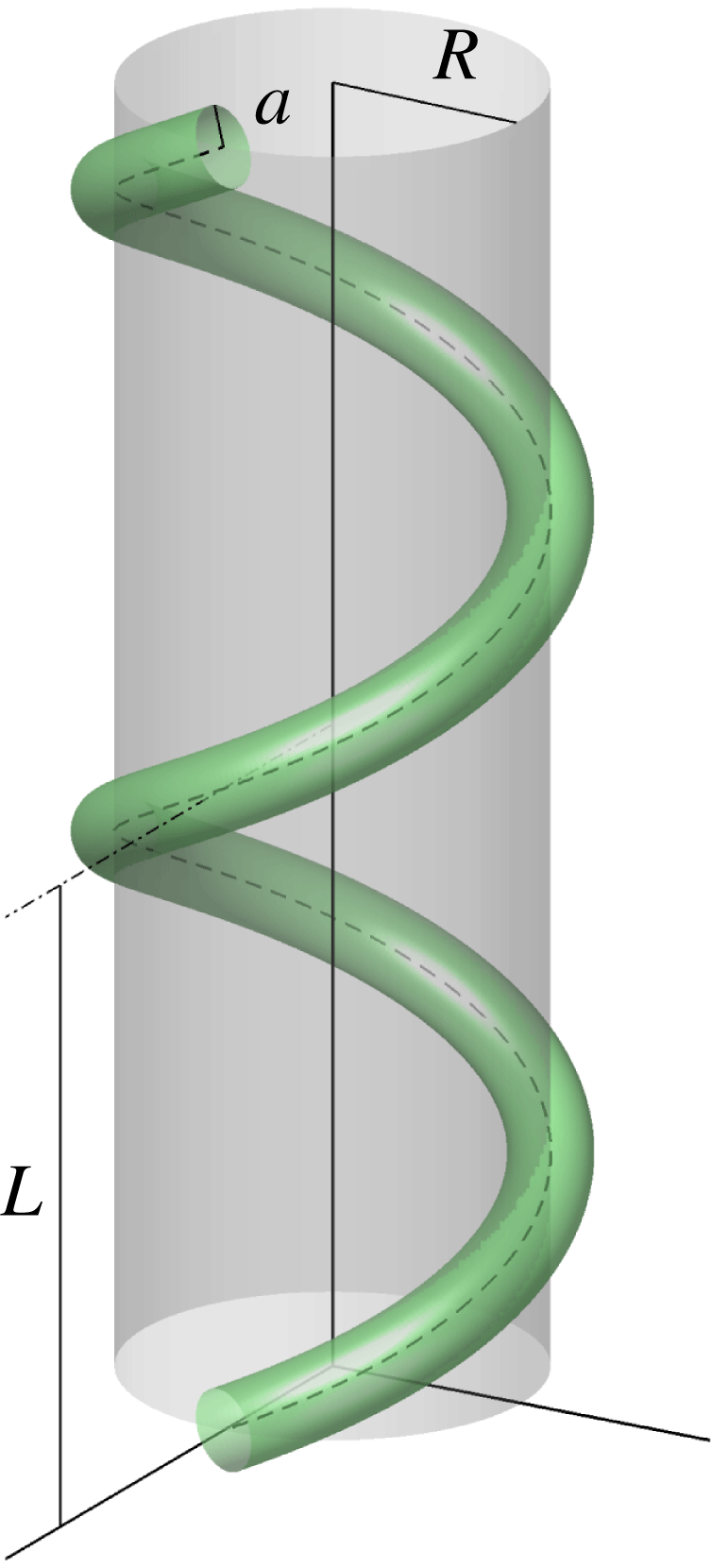
The realization that concentrated helical vortices are frequent features in natural and man-made flows has grown steadily since Parsons (Reference Parsons1901) discovered that ‘a small spiral vortex existed just behind the tips of the propeller blades’ used to generate the thrust needed to move a vessel. The theoretical study of helical vortices has an even longer history. Here, we highlight the earliest results, but see Ricca (Reference Ricca1994) for a detailed review of classical studies of the motion of a single helical vortex in an inviscid unbounded fluid (figure 1). Kelvin (Reference Thomson1880) found that one mode of vibration of a cylindrical vortex of uniform vorticity is a wave that deforms the vortex axis into a helix of small radius and large pitch, and that this wave propagates along the axis with constant speed. Fitzgerald (Reference Fitzgerald1899) assumed that this result was valid for helices of any pitch and radius and speculated about the flow induced by the vortex: ‘there will be, on the whole, a flow along the inside of the spiral, but the motion of the fluid is complex’. Joukowsky (Reference Joukowsky1912) showed that a helical vortex translates and rotates steadily without change of form and found that its velocity is approximately equal to the velocity of an osculating vortex ring; he further stated that any number of equal helical vortices symmetrically arranged with respect to a common axis form a steadily moving arrangement.
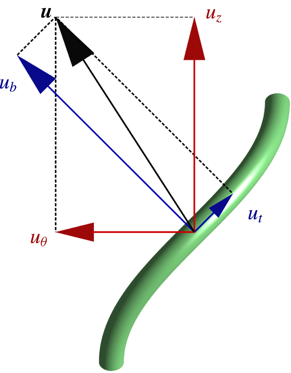
In the last two decades, there has been a renewed interest in helical vortices (Ricca Reference Ricca1994; Kuibin & Okulov Reference Kuibin and Okulov1998; Mezić, Leonard & Wiggins Reference Mezić, Leonard and Wiggins1998; Boersma & Wood Reference Boersma and Wood1999; Wood & Boersma Reference Wood and Boersma2001; Okulov Reference Okulov2004). Most of these works have concentrated on the binormal component of the vortex velocity and have implicitly or explicitly dismissed the tangential component (see figure 2). This component certainly contributes nothing to the time evolution of the Eulerian velocity and vorticity fields, but a vortex is essentially a Lagrangian object (see, e.g., Lugt Reference Lugt, Mueller, Roesner and Schmidt1979; Haller Reference Haller2005), and therefore the correct evaluation of the vortex motion requires the total velocity of the material particles that constitute the vortex. Furthermore, there are practical situations where the tangential velocity is important (Greenwell Reference Greenwell2003). Removal of this component leads to an error that may be small when the vortex has large pitch but becomes significant when the vortex has small pitch, as then the tangential component is approximately one third of the binormal one.
A segment of a thin helical vortex of cross-sectional radius
 $a$
. The vortex extends indefinitely in both directions and its centreline is a helix of pitch
 $L$
and radius
 $R$
lying on the surface of an imaginary supporting cylinder.

The objective of this paper is to obtain expressions for the linear and angular velocities of the vortex (
 $U$
and
 $\unicode[STIX]{x1D6FA}$
respectively) that are accurate over the whole range of pitch values for vortices of small cross-section (when compared with the radius of curvature of their centreline). Our methodology draws on the achievements of previous researchers of this subject.
-
(i) We compute the total velocity in terms of its axial and azimuthal components (Levy & Forsdyke Reference Levy and Forsdyke1928; Widnall Reference Widnall1972), and only later express it in terms of the binormal and tangential components in order to compare with previous analytic results (Boersma & Wood Reference Boersma and Wood1999; Greenwell Reference Greenwell2003).
-
(ii) As most authors have done before (Joukowsky Reference Joukowsky1912; Da Rios Reference Da Rios1916; Levy & Forsdyke Reference Levy and Forsdyke1928; Widnall Reference Widnall1972; Ricca Reference Ricca1994), we assume vortices of circular cross-section and uniform vorticity. These are mere approximations; in a steady solution of the Euler equations, the vorticity varies linearly with the distance from the centre of curvature and the cross-section differs slightly from a circle. However, they are good approximations when the radius of the cross-section is much smaller than the radius of curvature.
-
(iii) We compute the vortex velocity by averaging the velocity field at two diametrically opposed points on the surface of the vortex (Ricca Reference Ricca1994; Boersma & Wood Reference Boersma and Wood1999; Okulov Reference Okulov2004).
-
(iv) We use the approximation of Boersma & Wood (Reference Boersma and Wood1999) for the velocity field of a helical vortex obtained by Hardin (Reference Hardin1982).
Each of these approaches has been shown to be sound; our contribution is to use all of them in a consistent way in order to obtain new expressions for
 $U$
and
 $\unicode[STIX]{x1D6FA}$
.
The velocity of a helical vortex,
 $\boldsymbol{u}$
, represented as the sum of either the azimuthal and axial components (
 $u_{\unicode[STIX]{x1D703}}$
and
 $u_{z}$
respectively) or the tangential and binormal components (
 $u_{t}$
and
 $u_{b}$
respectively).

2 Theoretical results
A helical vortex is a thin tube of infinite length whose centreline is a helix of uniform pitch lying on the surface of an imaginary supporting cylinder (see figure 1). The centreline of the vortex is given, in Cartesian coordinates, as follows:
 $$\begin{eqnarray}\displaystyle & \displaystyle x=R\cos \unicode[STIX]{x1D703}, & \displaystyle\end{eqnarray}$$
 $$\begin{eqnarray}\displaystyle & \displaystyle y=R\sin \unicode[STIX]{x1D703}, & \displaystyle\end{eqnarray}$$
 $$\begin{eqnarray}\displaystyle & \displaystyle z=L\unicode[STIX]{x1D703}/2\unicode[STIX]{x03C0}, & \displaystyle\end{eqnarray}$$
where
 $\unicode[STIX]{x1D703}$
is the angle around the cylinder axis,
 $R$
is the radius of the helix and
 $L$
is the pitch of the helix.
On the circular cross-section of the vortex, the vorticity is uniform in magnitude and direction, which is parallel to the centreline tangent. The vortex thus has circulation
 $\unicode[STIX]{x1D6E4}=\unicode[STIX]{x03C0}a^{2}\unicode[STIX]{x1D714}$
, where
 $a$
is the radius of the cross-section and
 $\unicode[STIX]{x1D714}$
is the magnitude of the vorticity. The four parameters that uniquely define the vortex are then
 $\unicode[STIX]{x1D6E4}$
,
 $R$
,
 $L$
and
 $a$
, but, since the value of
 $\unicode[STIX]{x1D6E4}$
merely changes the time scale of the evolution, we are left with two dimensionless parameters, namely the vortex radius
 $\unicode[STIX]{x1D6FC}=a/R$
and the vortex pitch
 $\unicode[STIX]{x1D70F}=L/2\unicode[STIX]{x03C0}R$
.
Because of the geometry of the problem, the vortex velocity can be expressed in either cylindrical components,
 $u_{\unicode[STIX]{x1D703}}$
,
 $u_{z}$
, pointing in the azimuthal and axial directions respectively, or natural components,
 $u_{t}$
,
 $u_{b}$
, pointing in the tangent and binormal directions respectively (see figure 2). We will use cylindrical coordinates because the translation speed of the vortex,
 $U$
, equals the axial component of the velocity,
 $u_{z}$
, whereas the angular velocity of the vortex,
 $\unicode[STIX]{x1D6FA}$
, equals the azimuthal component divided by the helix radius,
 $u_{\unicode[STIX]{x1D703}}/R$
.
The velocity field produced by an infinitely thin helical vortex was obtained by Hardin (Reference Hardin1982), although some of his results were anticipated by Kawada (see Fukumoto, Okulov & Wood Reference Fukumoto, Okulov and Wood2015). Hardin’s solution, expressed in cylindrical coordinates, is divided into an interior field (valid inside the supporting cylinder) and an exterior field (valid outside the supporting cylinder). Here, we reproduce only the azimuthal and axial components needed for the calculation of the vortex motion,
 $$\begin{eqnarray}\displaystyle & \displaystyle u_{\unicode[STIX]{x1D703}}(r,\unicode[STIX]{x1D719})=\left\{\begin{array}{@{}ll@{}}{\displaystyle \frac{\unicode[STIX]{x1D6E4}R}{\unicode[STIX]{x03C0}rl}}S_{1}(r,\unicode[STIX]{x1D719}) & \text{if }r<R,\\[13.0pt] {\displaystyle \frac{\unicode[STIX]{x1D6E4}}{2\unicode[STIX]{x03C0}r}}+{\displaystyle \frac{\unicode[STIX]{x1D6E4}R}{\unicode[STIX]{x03C0}rl}}S_{2}(r,\unicode[STIX]{x1D719}) & \text{if }r>R,\end{array}\right. & \displaystyle\end{eqnarray}$$
 $$\begin{eqnarray}\displaystyle & \displaystyle u_{z}(r,\unicode[STIX]{x1D719})=\left\{\begin{array}{@{}ll@{}}{\displaystyle \frac{\unicode[STIX]{x1D6E4}}{2\unicode[STIX]{x03C0}l}}-{\displaystyle \frac{\unicode[STIX]{x1D6E4}R}{\unicode[STIX]{x03C0}l^{2}}}S_{1}(r,\unicode[STIX]{x1D719}) & \text{if }r<R,\\[13.0pt] -{\displaystyle \frac{\unicode[STIX]{x1D6E4}R}{\unicode[STIX]{x03C0}l^{2}}}S_{2}(r,\unicode[STIX]{x1D719}) & \text{if }r>R,\end{array}\right. & \displaystyle\end{eqnarray}$$
where
 $\unicode[STIX]{x1D719}=\unicode[STIX]{x1D703}-z/l$
,
 $l=L/2\unicode[STIX]{x03C0}$
and
 $$\begin{eqnarray}\displaystyle & \displaystyle S_{1}(r,\unicode[STIX]{x1D719})=\mathop{\sum }_{m=1}^{\infty }m\text{K}_{m}^{\prime }\left(\frac{mR}{l}\right)\text{I}_{m}\left(\frac{mr}{l}\right)\cos m\unicode[STIX]{x1D719}, & \displaystyle\end{eqnarray}$$
 $$\begin{eqnarray}\displaystyle & \displaystyle S_{2}(r,\unicode[STIX]{x1D719})=\mathop{\sum }_{m=1}^{\infty }m\text{K}_{m}\left(\frac{mr}{l}\right)\text{I}_{m}^{\prime }\left(\frac{mR}{l}\right)\cos m\unicode[STIX]{x1D719} & \displaystyle\end{eqnarray}$$
are Kapteyn-like series involving the modified Bessel functions
 $\text{K}_{m}$
and
 $\text{I}_{m}$
, and their corresponding derivatives
 $\text{K}_{m}^{\prime }$
and
 $\text{I}_{m}^{\prime }$
.
Since we are dealing with vortices of finite cross-section, it is possible to compute the velocity of the vortex by evaluating the velocity field at two diametrically opposed points on the surface of the tubular vortex. The uniformity of the vorticity on the cross-section guarantees that the average of these velocities is the actual velocity of the fluid particles lying on the centreline, i.e. the velocity of the vortex. This approach has been previously used by Ricca (Reference Ricca1994), Boersma & Wood (Reference Boersma and Wood1999) and Okulov (Reference Okulov2004) for the computation of the binormal component; here, we will use it for the computation of the axial and azimuthal components. For simplicity, we choose to evaluate the velocity at points
 $(r,\unicode[STIX]{x1D703},z)=(R\pm a,0,0)$
or, in helical coordinates,
 $(r,\unicode[STIX]{x1D719})=(R\pm a,0)$
. Therefore, the motion of the vortex is given by
 $$\begin{eqnarray}\displaystyle & \displaystyle U={\textstyle \frac{1}{2}}[u_{z}(R-a,0)+u_{z}(R+a,0)], & \displaystyle\end{eqnarray}$$
 $$\begin{eqnarray}\displaystyle & \displaystyle \unicode[STIX]{x1D6FA}=\frac{1}{2R}\left[u_{\unicode[STIX]{x1D703}}(R-a,0)+u_{\unicode[STIX]{x1D703}}(R+a,0)\right]. & \displaystyle\end{eqnarray}$$
A technical issue with this method is that the series
 $S_{1}$
and
 $S_{2}$
converge slowly, particularly when approaching the vortex itself, which hinders the computation of
 $U$
and
 $\unicode[STIX]{x1D6FA}$
. This problem was solved by Boersma & Wood (Reference Boersma and Wood1999), who eliminated the singularities from
 $S_{1}$
and
 $S_{2}$
for the two particular points needed in the computation of the motion,
 $$\begin{eqnarray}\displaystyle & \displaystyle S_{1}(R-a,0)=\frac{1}{4}\frac{\unicode[STIX]{x1D70F}^{2}}{(1+\unicode[STIX]{x1D70F}^{2})^{3/2}}\left(-\frac{2}{\unicode[STIX]{x1D716}}+\ln (\unicode[STIX]{x1D716})+\ln \left(\frac{\sqrt{1+\unicode[STIX]{x1D70F}^{2}}}{2}\right)\right)+\frac{\unicode[STIX]{x1D70F}}{2}-\frac{\unicode[STIX]{x1D70F}^{2}}{4}W(\unicode[STIX]{x1D70F}), & \displaystyle \nonumber\\ \displaystyle & & \displaystyle\end{eqnarray}$$
 $$\begin{eqnarray}\displaystyle & \displaystyle S_{2}(R+a,0)=\frac{1}{4}\frac{\unicode[STIX]{x1D70F}^{2}}{(1+\unicode[STIX]{x1D70F}^{2})^{3/2}}\left(\frac{2}{\unicode[STIX]{x1D716}}+\ln (\unicode[STIX]{x1D716})+\ln \left(\frac{\sqrt{1+\unicode[STIX]{x1D70F}^{2}}}{2}\right)\right)-\frac{\unicode[STIX]{x1D70F}^{2}}{4}W(\unicode[STIX]{x1D70F}), & \displaystyle\end{eqnarray}$$
where terms that tend to
 $0$
when
 $\unicode[STIX]{x1D716}\rightarrow 0$
have been omitted (
 $\unicode[STIX]{x1D716}=a/R_{c}$
, with the radius of curvature
 $R_{c}=R(1+\unicode[STIX]{x1D70F}^{2})$
) and
 $$\begin{eqnarray}\displaystyle & \displaystyle W(\unicode[STIX]{x1D70F})=\int _{0}^{\infty }\left[\frac{\sin ^{2}t}{(\unicode[STIX]{x1D70F}^{2}t^{2}+\sin ^{2}t)^{3/2}}-\frac{1}{(1+\unicode[STIX]{x1D70F}^{2})^{3/2}}\frac{H(1/2-t)}{t}\right]\text{d}t, & \displaystyle\end{eqnarray}$$
where
 $H(\cdot )$
the unit step function. Boersma & Wood (Reference Boersma and Wood1999) computed
 $W(\unicode[STIX]{x1D70F})$
by numerical quadrature for 21 values of
 $\unicode[STIX]{x1D70F}$
in the range
 $[0.01{-}10]$
and obtained approximate analytical forms for large values of
 $\unicode[STIX]{x1D70F}$
(giving less than 1 % error for
 $\unicode[STIX]{x1D70F}\geqslant 3$
) and for small values of
 $\unicode[STIX]{x1D70F}$
(giving less than 1 % error for
 $\unicode[STIX]{x1D70F}\leqslant 0.4$
). Here, we computed the value of
 $W(\unicode[STIX]{x1D70F})$
using the numerical method described by Boersma & Wood (Reference Boersma and Wood1999).
The substitution of these forms of
 $S_{1}$
and
 $S_{2}$
in (2.4)–(2.5) and the subsequent substitution of the resulting expressions for
 $u_{\unicode[STIX]{x1D703}}$
and
 $u_{z}$
in (2.8)–(2.9) give, after some algebra, the dimensionless linear and angular velocities of the vortex,
 $$\begin{eqnarray}\displaystyle & \displaystyle U^{\ast }=\frac{1}{(1+\unicode[STIX]{x1D70F}^{2})^{3/2}}(\ln (2/\unicode[STIX]{x1D716})-\ln (\sqrt{1+\unicode[STIX]{x1D70F}^{2}})+(1+\unicode[STIX]{x1D70F}^{2})^{3/2}W(\unicode[STIX]{x1D70F})), & \displaystyle\end{eqnarray}$$
 $$\begin{eqnarray}\displaystyle \unicode[STIX]{x1D6FA}^{\ast } & = & \displaystyle \frac{\unicode[STIX]{x1D70F}}{(1+\unicode[STIX]{x1D70F}^{2})^{3/2}}\nonumber\\ \displaystyle & & \displaystyle \times \,\left(\frac{2(1+\unicode[STIX]{x1D70F}^{2})+\ln (2/\unicode[STIX]{x1D716})-\ln (\sqrt{1+\unicode[STIX]{x1D70F}^{2}})-(1+\unicode[STIX]{x1D70F}^{2})^{3/2}(2/\unicode[STIX]{x1D70F}-W(\unicode[STIX]{x1D70F}))}{\unicode[STIX]{x1D716}^{2}(1+\unicode[STIX]{x1D70F}^{2})^{2}-1}\right).\nonumber\\ \displaystyle & & \displaystyle\end{eqnarray}$$
The expression for
 $\unicode[STIX]{x1D6FA}^{\ast }$
may be simplified using the assumption
 $\unicode[STIX]{x1D6FC}^{2}\ll 1$
,
 $$\begin{eqnarray}\displaystyle & \displaystyle \unicode[STIX]{x1D6FA}^{\ast }\approx -\frac{\unicode[STIX]{x1D70F}}{(1+\unicode[STIX]{x1D70F}^{2})^{3/2}}\left(\ln (2/\unicode[STIX]{x1D716})-\ln (\sqrt{1+\unicode[STIX]{x1D70F}^{2}})+(1+\unicode[STIX]{x1D70F}^{2})^{3/2}(W(\unicode[STIX]{x1D70F})-2/\unicode[STIX]{x1D70F})+2(1+\unicode[STIX]{x1D70F}^{2})\right). & \displaystyle \nonumber\\ \displaystyle & & \displaystyle\end{eqnarray}$$
The dimensional vortex velocities are obtained by multiplying
 $U^{\ast }$
by
 $\unicode[STIX]{x1D6E4}/4\unicode[STIX]{x03C0}R$
and
 $\unicode[STIX]{x1D6FA}^{\ast }$
by
 $\unicode[STIX]{x1D6E4}/4\unicode[STIX]{x03C0}R^{2}$
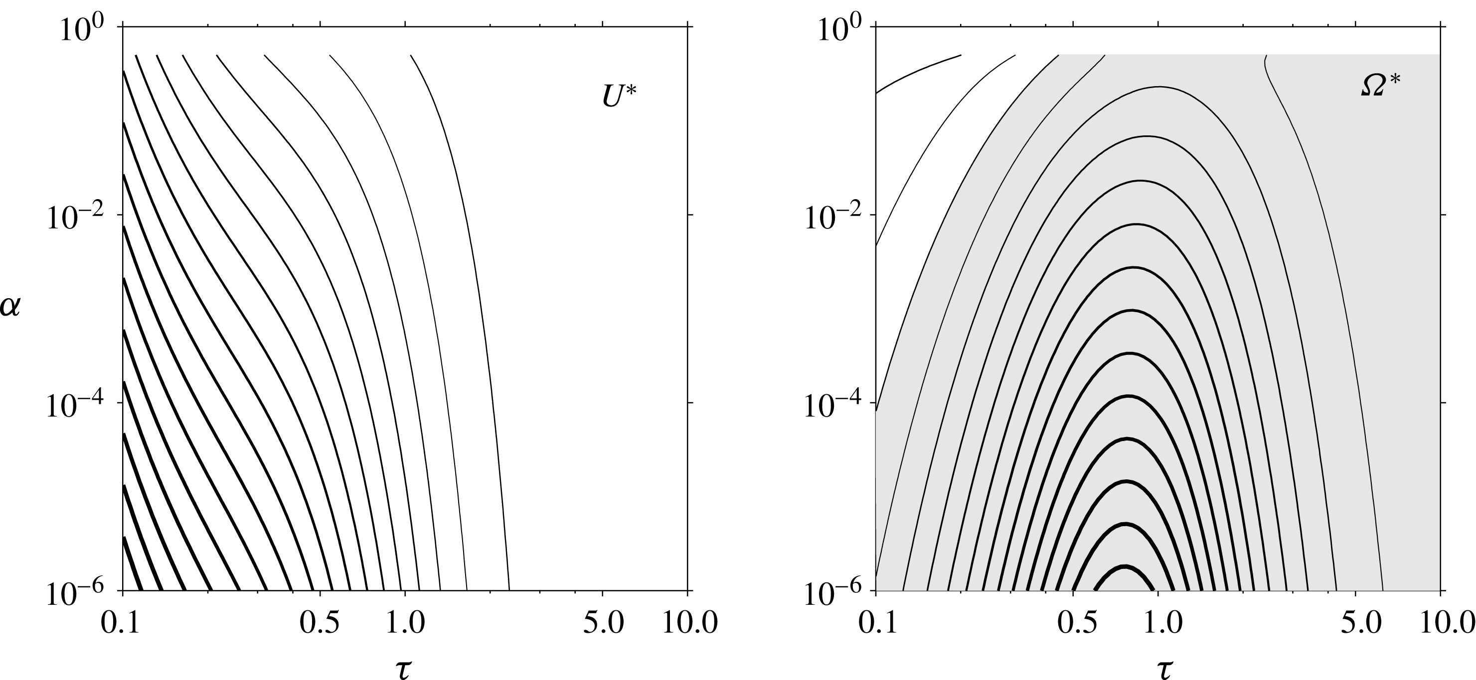
. Figure 3 shows
 $U^{\ast }$
and
 $\unicode[STIX]{x1D6FA}^{\ast }$
(computed using (2.14)) in the region
 $10^{-6}<\unicode[STIX]{x1D6FC}<0.4$
and
 $0.1<\unicode[STIX]{x1D70F}<10$
. Helical vortices always translate in the direction of the axial component of the vorticity; they do so with a velocity that increases as their pitch
 $\unicode[STIX]{x1D70F}$
and radius
 $\unicode[STIX]{x1D6FC}$
decrease.
The non-dimensional linear and angular velocities of a helical vortex (
 $U^{\ast }$
and
 $\unicode[STIX]{x1D6FA}^{\ast }$
respectively) as functions of its pitch and radius (
 $\unicode[STIX]{x1D70F}$
and
 $\unicode[STIX]{x1D6FC}$
respectively). Thicker contours indicate higher absolute values of
 $U^{\ast }$
or
 $\unicode[STIX]{x1D6FA}^{\ast }$
; the grey area indicates the region of the parameter space where
 $\unicode[STIX]{x1D6FA}^{\ast }$
is negative (clockwise rotation of the helix). The smallest value of
 $U^{\ast }$
represented by a contour is 1 and the contour interval is 1.25; the smallest value of
 $\unicode[STIX]{x1D6FA}^{\ast }$
represented by a contour is
 $-$
5.2 and the contour interval is 0.4.

Helical vortices generally rotate opposite to the azimuthal component of the vorticity, i.e. clockwise when seen from the direction in which the vortices translate. This occurs because the centreline of the vortices is a right-handed helix and the binormal velocity is generally much larger than the tangential one (see figure 2). For a fixed radius
 $\unicode[STIX]{x1D6FC}$
, helical vortices rotate with an angular velocity that has a maximum absolute value when their pitch
 $\unicode[STIX]{x1D70F}$
is approximately one; for a fixed pitch
 $\unicode[STIX]{x1D70F}$
, the angular velocity increases in magnitude as the radius of the vortices
 $\unicode[STIX]{x1D6FC}$
decreases. The positive values of
 $\unicode[STIX]{x1D6FA}^{\ast }$
in the upper left corner of figure 3 are explained as follows:
 $u_{\unicode[STIX]{x1D703}}\rightarrow 0$
as
 $\unicode[STIX]{x1D70F}\rightarrow 0$
, whereas
 $u_{t}$
grows with
 $\unicode[STIX]{x1D6FC}$
; therefore, relatively thick vortices of small pitch rotate in the anti-clockwise sense.
It should be noted that the translation speed
 $U^{\ast }$
behaves as the helix curvature,
 $1/R(1+\unicode[STIX]{x1D70F}^{2})$
, which has a maximum value (
 $1/R$
) when
 $\unicode[STIX]{x1D70F}=0$
and then decreases to zero as
 $\unicode[STIX]{x1D70F}$
goes to infinity. Similarly, the magnitude of the rotation speed
 $\unicode[STIX]{x1D6FA}^{\ast }$
behaves as the helix torsion,
 $\unicode[STIX]{x1D70F}/R(1+\unicode[STIX]{x1D70F}^{2})$
, which grows from zero when
 $\unicode[STIX]{x1D70F}=0$
to its maximum value (
 $1/2R$
) when
 $\unicode[STIX]{x1D70F}=1$
and then decreases to zero as
 $\unicode[STIX]{x1D70F}$
goes to infinity.
The natural components of the vortex velocity are related to the cylindrical components by the following expressions:
 $$\begin{eqnarray}\displaystyle & \displaystyle U_{b}=\frac{U-\unicode[STIX]{x1D70F}R\unicode[STIX]{x1D6FA}}{\sqrt{1+\unicode[STIX]{x1D70F}^{2}}},\quad U_{t}=\frac{\unicode[STIX]{x1D70F}U+R\unicode[STIX]{x1D6FA}}{\sqrt{1+\unicode[STIX]{x1D70F}^{2}}}. & \displaystyle\end{eqnarray}$$
Using here the values of
 $U$
and
 $\unicode[STIX]{x1D6FA}$
given by (2.13) and (2.15), we obtain the binormal and tangential components of the vortex velocity,
 $$\begin{eqnarray}\displaystyle & \displaystyle U_{b}^{\ast }=\frac{1}{1+\unicode[STIX]{x1D70F}^{2}}(\ln (2/\unicode[STIX]{x1D716})-\ln (\sqrt{1+\unicode[STIX]{x1D70F}^{2}})+(1+\unicode[STIX]{x1D70F}^{2})^{3/2}W(\unicode[STIX]{x1D70F})-2\unicode[STIX]{x1D70F}\sqrt{1+\unicode[STIX]{x1D70F}^{2}}+2\unicode[STIX]{x1D70F}^{2}), & \displaystyle \nonumber\\ \displaystyle & & \displaystyle\end{eqnarray}$$
 $$\begin{eqnarray}\displaystyle & \displaystyle U_{t}^{\ast }=\frac{2(\sqrt{1+\unicode[STIX]{x1D70F}^{2}}-\unicode[STIX]{x1D70F})}{1+\unicode[STIX]{x1D70F}^{2}}. & \displaystyle\end{eqnarray}$$
These must be multiplied by
 $\unicode[STIX]{x1D6E4}/4\unicode[STIX]{x03C0}R$
to obtain the dimensional velocities. If we write the binormal velocity in the form
 $$\begin{eqnarray}\displaystyle & \displaystyle U_{b}=\frac{\unicode[STIX]{x1D6E4}}{4\unicode[STIX]{x03C0}R}\frac{1}{1+\unicode[STIX]{x1D70F}^{2}}\left(\log \left(\frac{1}{\unicode[STIX]{x1D716}}\right)+C\right), & \displaystyle\end{eqnarray}$$
we find that
 $C$
, the so-called remainder, coincides with the result of Boersma & Wood (Reference Boersma and Wood1999). Similarly,
 $U_{t}^{\ast }/2$
gives the result obtained by Greenwell (Reference Greenwell2003) for the tangential velocity at the initial point of a semi-infinite helical vortex.
3 Comparison with numerical results
We verified (2.13) and (2.14) by computing the velocity of the vortex by numerical integration of the Helmholtz formula,
 $$\begin{eqnarray}\displaystyle & \displaystyle \boldsymbol{u}(\boldsymbol{x})=-{\displaystyle \frac{1}{4\unicode[STIX]{x03C0}}}\int {\displaystyle \frac{[\boldsymbol{x}-\boldsymbol{x}^{\prime }]\times \unicode[STIX]{x1D74E}}{|\boldsymbol{x}-\boldsymbol{x}^{\prime }|^{3}}}\,\text{d}V, & \displaystyle\end{eqnarray}$$
and the Rosenhead–Moore approximation to the Biot–Savart law (e.g. Saffman Reference Saffman1995),
 $$\begin{eqnarray}\displaystyle & \displaystyle \boldsymbol{u}(\boldsymbol{x})=-{\displaystyle \frac{\unicode[STIX]{x1D6E4}}{4\unicode[STIX]{x03C0}}}\int {\displaystyle \frac{[\boldsymbol{x}-\boldsymbol{r}(s)]\times \text{d}\boldsymbol{r}}{\left(|\boldsymbol{x}-\boldsymbol{r}(s)|^{2}+\unicode[STIX]{x1D707}^{2}a^{2}\right)^{3/2}}}, & \displaystyle\end{eqnarray}$$
where
 $a$
is the radius of the cross-section of the tubular vortex and
 $\unicode[STIX]{x1D707}$
is a parameter that depends on the vortex local structure, i.e. its vorticity distribution, curvature and torsion. By our definition, a helical vortex has the same local structure everywhere; therefore,
 $\unicode[STIX]{x1D707}$
is a constant whose value must be determined. This is usually done by choosing
 $\unicode[STIX]{x1D707}$
so that the integral (3.2) produces results in agreement with a known solution obtained with a different method (see, e.g., Saffman Reference Saffman1995). Here, we use
 $\unicode[STIX]{x1D707}=\text{e}^{-3/4}$
because this value leads to the correct velocity for a vortex ring of uniform vorticity, constant curvature and zero torsion; this choice may thus be expected to give a good approximation for a helical vortex of uniform vorticity, constant curvature and constant torsion.
We evaluated the velocity at
 $(x,y,z)=(R,0,0)$
by integrating (3.1) and (3.2) in the interval
 $-nL<z<nL$
, where
 $n$
is an integer and
 $L$
is the dimensional pitch. In the computation of the Rosenhead–Moore integral, we used a single filament represented by
 $M$
straight segments per helix coil. In the computation of the Helmholtz integral, we used 100 filaments, each represented by
 $M$
straight segments per helix coil; none of these filaments coincided with the vortex centreline, so, in contrast to the Biot–Savart case, there was no need to smooth out the singularity and, consequently, there is no free tuning parameter in (3.1). The value of
 $M$
varied between
 $10^{3}$
and
 $10^{4}$
depending on the helix pitch
 $L$
. We chose
 $n$
large enough to make the relative difference between the integrals computed with
 $n$
and
 $n+1$
less than 0.0001 %.
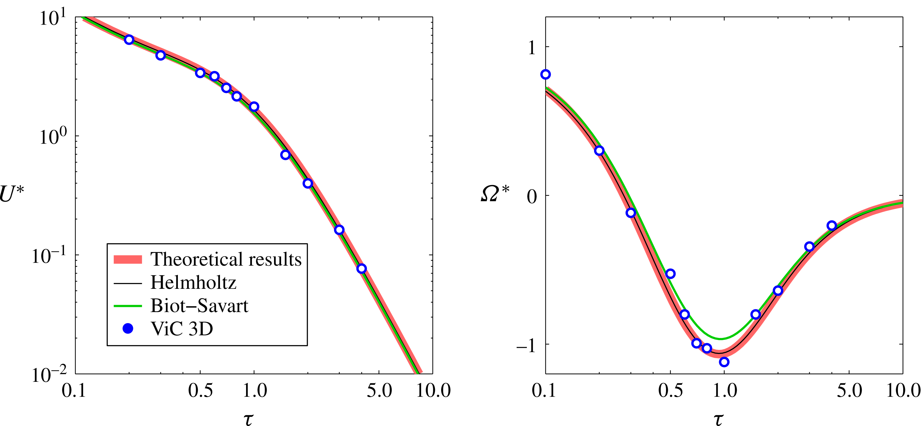
Linear and angular velocities,
 $U^{\ast }$
and
 $\unicode[STIX]{x1D6FA}^{\ast }$
respectively, as functions of the vortex pitch (
 $\unicode[STIX]{x1D70F}$
) for a given vortex radius (
 $\unicode[STIX]{x1D6FC}=0.1$
).

Figure 4 shows the linear and angular velocities,
 $U^{\ast }$
and
 $\unicode[STIX]{x1D6FA}^{\ast }$
respectively, as functions of the vortex pitch (
 $0.1<\unicode[STIX]{x1D70F}<10$
) for a given vortex radius (
 $\unicode[STIX]{x1D6FC}=0.1$
). There is very close agreement between the velocities computed with (2.13)–(2.14) and the Helmholtz integral (the relative difference is approximately
 $0.25\,\%$
). The difference between the theoretical velocities and the velocities obtained with the Rosenhead–Moore calculations is larger, approximately 4.5 %, with the largest values occurring around
 $\unicode[STIX]{x1D70F}=1$
. This is noteworthy because
 $\unicode[STIX]{x1D70F}=1$
is the point of highest torsion, and the value of the free parameter in the Rosenhead–Moore kernel,
 $\unicode[STIX]{x1D707}=\text{e}^{-3/4}$
, was chosen to give the correct result for a vortex of zero torsion.
A third way of verifying our theoretical results was by computing the actual motion of a helical vortex using a vortex-in-cell model that solves the Euler equations in a triple-periodic box (see, e.g., Suaza Jaque & Velasco Fuentes Reference Suaza Jaque and Velasco Fuentes2017). We obtained the velocities by computing the linear and angular displacements of individual vortical particles, dividing those displacements by the elapsed time and taking the average over all particles (
 ${\approx}250\,000$
). These velocities behave more irregularly than those obtained with the Helmholtz integral or the Rosenhead–Moore approximation, but the differences from the theoretical results are in the range 0 %–5 %. More importantly, these simulations verified the validity of the assumptions on which the analytical calculations are based; namely that, throughout the evolution of the vortex, its centreline remains a helix, its cross-section a circle and its vorticity uniform and parallel to the centreline. These three assumptions proved to be right to a very good approximation.
4 Comparison with previous results
Joukowsky (Reference Joukowsky1912) and Da Rios (Reference Da Rios1916) found that, to the order of approximation they used, the velocity is entirely in the binormal direction. They found the binormal velocity,
 $U_{b}$
, to be given by
 $$\begin{eqnarray}\displaystyle U_{b}=\left\{\begin{array}{@{}ll@{}}{\displaystyle \frac{\unicode[STIX]{x1D6E4}}{4\unicode[STIX]{x03C0}R_{c}}}\log \left({\displaystyle \frac{2R_{c}}{a}}\right) & \text{(Joukowsky 1912)},\\[15.60004pt] {\displaystyle \frac{\unicode[STIX]{x1D6E4}}{4\unicode[STIX]{x03C0}R_{c}}}\log \left({\displaystyle \frac{R}{a}}\right) & \text{(Da Rios 1916)},\end{array}\right.\end{eqnarray}$$
where
 $R_{c}=R(1+\unicode[STIX]{x1D70F}^{2})$
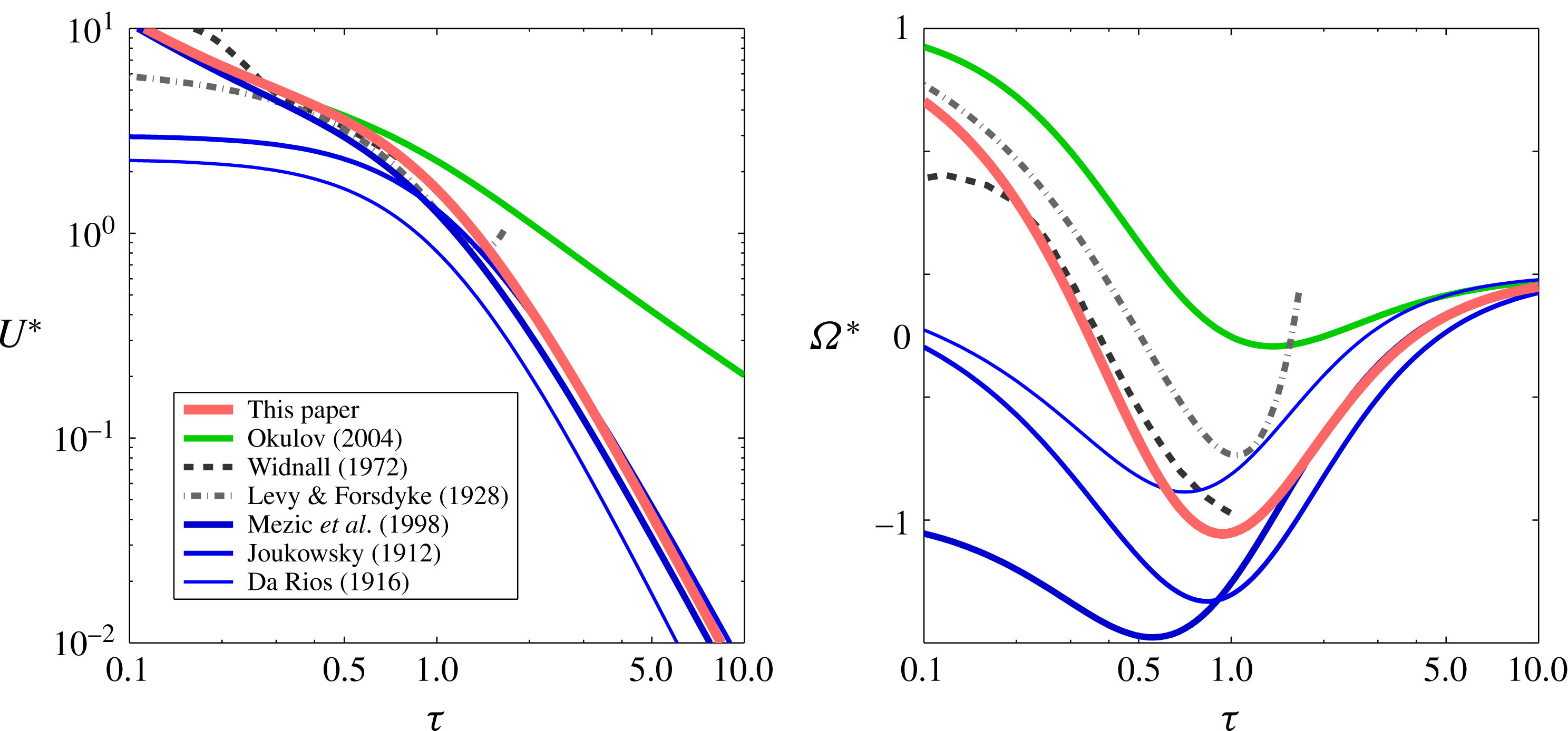
is the radius of curvature. It should be noted that these formulae are variations of the localized induction approximation first enunciated by Schwedoff (Reference Schwedoff1887) and later mathematically formalized by Da Rios (Reference Da Rios1906). We decomposed these velocities in cylindrical components in order to compute
 $U^{\ast }$
and
 $\unicode[STIX]{x1D6FA}^{\ast }$
(see the thin blue lines in figure 5); they are in reasonably good agreement with (2.13)–(2.14), shown in red thick lines, for
 $\unicode[STIX]{x1D70F}>2$
only.
Levy & Forsdyke (Reference Levy and Forsdyke1928) and Widnall (Reference Widnall1972) computed the linear velocity
 $U$
and angular velocity
 $\unicode[STIX]{x1D6FA}$
of helical vortices of small pitch (in the ranges
 $0.25<\unicode[STIX]{x1D70F}<1.25$
and
 $0.1<\unicode[STIX]{x1D70F}<1$
respectively). Levy & Forsdyke (Reference Levy and Forsdyke1928) avoided the singularity in the Biot–Savart law by evaluating part of the integral near, instead of on, the filament; Widnall (Reference Widnall1972) obtained the vortex velocity using the cutoff method and matched asymptotic expansions. In the range
 $0.3<\unicode[STIX]{x1D70F}<1$
, the results of Levy & Forsdyke (Reference Levy and Forsdyke1928) and Widnall (Reference Widnall1972), shown by dashed and dash-dotted lines in figure 5, are in better agreement with (2.13)–(2.14) than any earlier or later result.
Linear and angular velocities,
 $U^{\ast }$
and
 $\unicode[STIX]{x1D6FA}^{\ast }$
respectively, as functions of the vortex pitch (
 $\unicode[STIX]{x1D70F}$
) for a given vortex radius (
 $\unicode[STIX]{x1D6FC}=0.1$
).

Ricca (Reference Ricca1994), Mezić et al. (Reference Mezić, Leonard and Wiggins1998) and Boersma & Wood (Reference Boersma and Wood1999) argued that the tangential velocity is unimportant and computed the binormal velocity (
 $U_{b}$
) only. Mezić et al. (Reference Mezić, Leonard and Wiggins1998) decomposed
 $U_{b}$
to obtain
 $U^{\ast }$
and
 $\unicode[STIX]{x1D6FA}^{\ast }$
; the former shows reasonable agreement with (2.13) for all values of the vortex pitch, the latter shows good agreement with (2.14) for
 $\unicode[STIX]{x1D70F}>1$
only. It should be noted that while
 $U_{b}$
is sufficient to determine the time evolution of the Eulerian velocity and vorticity fields, neglect of the tangential velocity (
 $U_{t}$
) leads to error when studying particle motion in the vicinity of the vortex; see, e.g., the video https://youtu.be/FmrqtHK7wVM (Velasco Fuentes Reference Velasco Fuentes2015). Even more seriously, as the same video shows, neglect of
 $U_{t}$
leads to slippage of irrotational fluid in contact with vortical fluid, i.e. to the appearance of a vortex sheet at the vortex boundary.
Finally, the results of Okulov (Reference Okulov2004) for the binormal component are in good agreement with our results, but his results for
 $U\ast$
and
 $\unicode[STIX]{x1D6FA}\ast$
, shown by green lines in figure 5, differ greatly from ours as a consequence of the use of inconsistent assumptions, as explained below. In what follows, the prefixes ‘R’ and ‘O’ indicate equations in Ricca (Reference Ricca1994) and Okulov (Reference Okulov2004) respectively. Equation (O4.4), which gives
 $\unicode[STIX]{x1D6FA}$
as a function of
 $\unicode[STIX]{x1D70F}$
and
 $U_{b}$
, was obtained using (O2.4) and transformation relations between cylindrical and natural components (see, e.g., (R4.1)). Then,
 $U_{b}$
was computed under the assumption that the vorticity is uniform on the vortex cross-section (see (O4.6) and (R4.12)). A conflict exists because (O2.4) implies (O2.9), which means that the vorticity is parallel to helical lines of constant dimensional pitch (
 $l=L/2\unicode[STIX]{x03C0}$
). Such a vorticity field cannot be uniform on the vortex cross-section; thus, (O4.4) gives an incorrect value of
 $\unicode[STIX]{x1D6FA}$
. The same conflicting assumptions are used by Okulov & Sørensen (Reference Okulov and Sørensen2007, Reference Okulov and Sørensen2010).
5 Conclusions
We have found new expressions for the linear and angular velocities of helical vortices that have, to leading order, uniform vorticity and circular cross-section. These expressions are valid for vortices of any pitch when their cross-sectional radius is much smaller than the helix radius (
 $\unicode[STIX]{x1D6FC}^{2}\ll 1$
).
Numerical computations of the linear and angular velocities of a helical vortex using the exact Helmholtz formula, the approximated Rosenhead–Moore integral and a triple-periodic vortex-in-cell model show that our theoretical results are correct (within the limits of our assumptions) over the whole range of the vortex parameters. Previous analytical formulae generally give good approximations for vortices of large pitch only (say
 $\unicode[STIX]{x1D70F}>5$
), the most notable exception being Widnall (Reference Widnall1972), whose results agree very well with our theoretical formulae and numerical calculations in the range
 $0.3<\unicode[STIX]{x1D70F}<1$
.
Acknowledgements
I gratefully acknowledge Professor D. H. Wood for bringing to my attention the early work of S. Kawada on the velocity field of a helical vortex, and the anonymous referees for their comments and criticisms on previous versions of this paper. This research was supported by CONACyT (México) under grant number 169574.