A. Initial microstructure and true stress–true strain curves

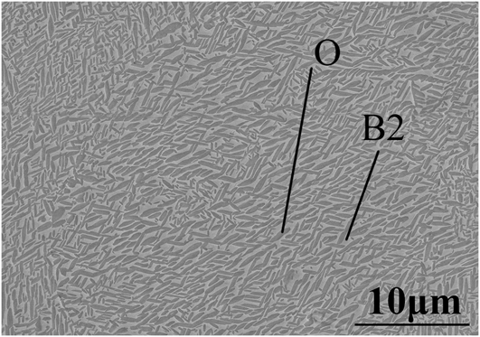
The initial microstructure of the Ti–22Al–25Nb alloy is shown in Fig. 1. The grey matrix phase is B2 phase and the dark phase is the strengthening phase. Energy dispersive X-ray spectroscopy analysis was used to confirm the composition. The result shows that the at.% of titanium and aluminum are 52.0% and 23.9%, respectively, revealing that the lamellar phase is O phase rather than α₂ phase. It can be seen that O phase is uniformly distributed in the B2 matrix.

FIG. 1.

SEM image of the initial microstructure for the Ti–22Al–25Nb alloy.

The true stress–true stain curves under different strain rates and temperatures are shown in Fig. 2. During hot compression process, the flow stress increases sharply, until to the peak at a relatively low strain (lower than 0.05), and then decreases slightly. Some curves may experience steady-flow behaviors at last. It should be noted that the true stress–true strain curves can be divided into two types.

FIG. 2.

True stress versus true stain curves for the Ti–22Al–25Nb alloy at (a) 930 °C, (b) 980 °C, (c) 1030 °C, and (d) 1080 °C.

One type exhibits a sharp stress peak followed by slightly decreasing flow behavior. Some curves may display a steady-state flow ultimately, owing to the dynamic balance between the work hardening and the flow softening, which is mainly induced by DRX or lamellar globularization.^{Reference Li, Huang, Meng, Geng and Cui17}

The other type undergoes a severe drop after the stress peak and then increases slightly to the upper yield stress, followed by a decrease in stress. The work hardening and the rapid propagation of mobile dislocations may account for the sharp increase and the rapid drop, while the following slow increase of flow stress is mainly associated with the interaction of strain hardening with dynamic recovery.^{Reference Wang, Hamasaki, Yamamura, Yamauchi, Maeda, Shirai and Yoshida18,Reference Jia, Zeng, Zhou, Liu and Wang19} As the strain is continuously increased, the softening mechanism plays a dominant role.

It can be seen from Fig. 2 that with the increase of the deformation rate, the value of the stress peak is also increased, as well as the corresponding strain. Meanwhile, the stress peak tends to shift to the opposite direction as the deformation temperature is increased. To further analyze the hot deformation behavior of the alloy, the constitutive equation, the thermal process map, and the DRX kinetics model will be built up.

B. Constitutive equation

Empirical function associated with activation energy has been used to investigate the hot deformation behavior of alloys.^{Reference Dehghan, Abbasi and Momeni20–Reference McQueen and Imbert22} Using a hyperbolic-sine equation proposed by Sellars and Tegart, the relationship between flow stress, strain rate, and deformation temperature during hot deformation at a given strain can be expressed as follows^{Reference Sellars and Tegart23}:

(2)$$Z = \dot \varepsilon \exp \left( {{Q \over {RT}}} \right) = A{\left[ {\sinh \left( {\alpha {\sigma _{\rm{p}}}} \right)} \right]^n}\quad ,$$

where σ is the flow stress (MPa), ε is the strain rate (s⁻¹), T is the absolute deformation temperature (K), Q is the apparent activation energy of deformation (kJ/mol), R is the gas constant (kJ/mol K), and n, α, and A are constants related to the material.

By taking natural logarithm of both sides in Eq. (2), it gives:

(3)$$\ln Z = \ln \dot \varepsilon + {Q \over {RT}} = \ln A + n\ln \left[ {\sinh \left( {\alpha {\sigma _{\rm{p}}}} \right)} \right]$$

and [sinh(ασ_p)] can be expressed as follows^{Reference Meng, Li, Li, Huang and Nie24–Reference Sellars and Tegart27}:

(4)$$\left[ {\sinh \left( {\alpha \sigma } \right)} \right] = \left\{ {\matrix{ {{\sigma ^n}} & {\alpha \sigma \,\lt\, 0.8} \cr {\exp \left( {\beta \sigma } \right)} & {\alpha \sigma > 1.2} \cr} } \quad ,$$

where β and n are all constants and α = β/n.

It is necessary to define the value of β, which can be calculated through Eq. (2) and Eq. (4)^{Reference McQueen and Imbert22}

(5)$$\dot \varepsilon = {A_1}\mathop {{\sigma _{\rm{p}}}}\nolimits^n \,\exp \left( {{{ - Q} \over {RT}}} \right)$$

(6)$$\dot \varepsilon = {A_2}\,\exp \left( {\beta {\sigma _{\rm{p}}}} \right)\exp \left( {{{ - Q} \over {RT}}} \right)$$

Taking natural logarithm of both sides of Eq. (5) and Eq. (6), β and n can be defined as:

(7)$$n = {{\partial \ln \,\dot \varepsilon } \over {\partial \ln \,{\sigma _{\rm{p}}}}}\quad ,$$

(8)$$\beta = {{\partial \ln \,\dot \varepsilon } \over {\partial {\sigma _{\rm{p}}}}}\quad .$$

From Figs. 3(a) and 3(b), the value of stress multiplier n and β can be determined by using the average values of β and n at different T, the stress multiplier α is determined as 0.00753.

FIG. 3.

Linear fittings for (a) ln ε versus ln σ, (b) ln ε versus σ; (c) ln ε versus ln[sinh(ασ)] and (d) ln[sinh(ασ)] versus T ⁻¹.

The Q can be calculated as follows by Eq. (3):

(9)$$Q = R{\left\{ {{{\partial \ln \,\dot \varepsilon } \over {\partial \ln \left[ {\sinh \left( {\alpha {\sigma _{\rm{p}}}} \right)} \right]}}} \right\}_T}\left\{ {{{\partial \ln \left[ {\sinh \left( {\alpha {\sigma _{\rm{p}}}} \right)} \right]} \over {\partial \left( {{1 \mathord{\left/ {\vphantom {1 T}} \right. \kern-\nulldelimiterspace} T}} \right)}}} \right\}\quad .$$

Figures 3(c) and 3(d) can be used to evaluate other parameters,^{Reference Sha28} and the constants values of the explored alloy are listed in Table II.

TABLE II.

Values of material constants and activation energy for the investigated Ti-22Al-25Nb alloy.

The constitutive equation of Ti–22Al–25Nb can be expressed as follows:

$$Z = \dot \varepsilon \,\exp \left( {{{621700} \over {RT}}} \right) = {{\rm{e}}^{54.21}}{\left[ {\sinh \left( {0.00753{\sigma _{\rm{p}}}} \right)} \right]^{3.156}}\quad .$$

Through the constitutive equation, the relationship between the peak stress, the deformation rate, and the processing temperature of the Ti–22Al–25Nb alloy can be analyzed quantitatively. Overall, with the increase of strain rate and the decrease of deformation temperature, the stress peak is increased, which is consistent with the true stress–true strain curve.

The constitutive equation is used to represent the dynamic response of the materials to thermal deformation, which reveals the relationship between true stress, strain rate, and the deformation temperature. It is worth mentioning that the microstructure evolution has a great influence on the property of the alloy, which can hardly be judged by a single equation. So it is necessary to establish processing maps for further analysis.

C. Processing maps

Based on the DMM, processing maps may clarify different domains during plastic deformation, which can facilitate optimization of the hot working processes.^{Reference Prasad, Gegel, Doraivelu, Malas, Morgan, Lark and Barker11}

A processing map of the Ti–22Al–25Nb alloy under the true strain of 0.6 is shown in Fig. 4. In the processing map, the contour numbers represent the efficiency of power dissipation (η), and the shaded areas indicate the instability regions, where there are four different domains. The first domain is the stable region and characterized by the temperature range of 980–1030 °C and the strain rate from 0.1 s⁻¹ to 0.001 s⁻¹, with a peak efficiency of 22% occurring at about 1010 °C and 0.03 s⁻¹. However, the other three domains are unstable regions, which are scattered on the edges of the processing map.

FIG. 4.

Processing map of Ti–22Al–25Nb alloy at a strain of 0.6.

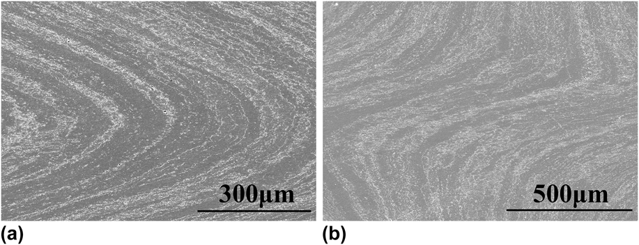
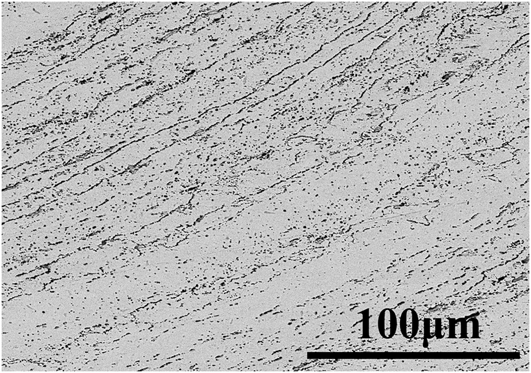
To explore the reasons for occurrence of unstable regions, specimens in these three regions are examined, revealing that all of them have adiabatic shear bands, which are shown in Fig. 5. More details of the adiabatic shear bands are shown in Fig. 6. Globular O phase grains are precipitated along shear zones. The deformation heating generated during the rapid hot deformation cannot be released in time, giving rise to the localized temperature.

FIG. 5.

Microstructures occurring in the instability domain of Ti–22Al–25Nb alloy, (a) shear bands at the edge of the specimen and (b) in the center of the specimen.

FIG. 6.

BSE image of the shear band.

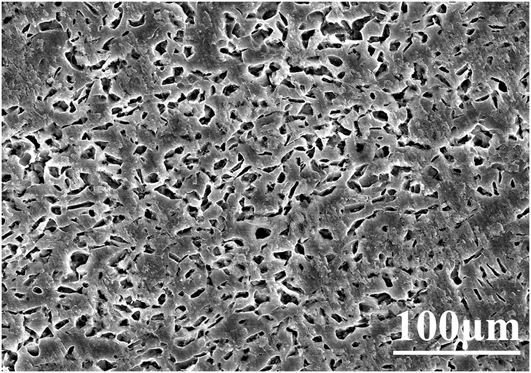
Microstructure examination of stable regions indicates that the factors contributing to high power dissipation are different. At low temperature, the stable region is mainly related to the lamellar globularization,^{Reference Li, Huang, Meng, Geng and Cui17} as shown in Fig. 7, while at high temperature is mainly involved in DRX.^{Reference Sun, Zeng, Zhao, Zhang, Shu and Zhou29} Meanwhile, the shape of B2 grains after deformation is also changed, which is flattened in a direction vertical to the compression direction (see Fig. 8).

FIG. 7.

SEM image of lamellar globularization at 980 °C and 0.001 s⁻¹.

FIG. 8.

OM image of the deformation B2 grains at 1080 °C and 0.001 s⁻¹.

D. Kinetics of DRX

During hot deformation, the tangled dislocations would lead to work hardening, and when the amount of dislocations reaches a certain level, the DRX would be initiated.^{Reference Cheng, Chang, Tang, Kou and Li30} As the strain is increased, some curves finally exhibit steady-state flows, implying the occurrence of the full evolution of DRX. Based on the Avrami-type equation,^{Reference Xu, Hu and Sun15,Reference Lv, Peng, Shi, Tang and Pan16,Reference Cheng, Chang, Tang, Kou and Li30–Reference Liu, Cui and Ruan32} the kinetics model of DRX can be given as:

(10)$${X_{{\rm{DRX}}}} = 1 - \exp \left[ { - k{{\left( {{{\varepsilon - {\varepsilon _{\rm{c}}}} \over {\varepsilon {\rm{*}}}}} \right)}^n}} \right]$$

(11)$${X_{{\rm{DRX}}}} = {{\sigma - {\sigma _{\rm{p}}}} \over {{\sigma _{{\rm{ss}}}} - {\sigma _{\rm{p}}}}}\quad {\rm{,}}$$

where X _DRX is the volume fraction of DRX grains, ε* is the strain for maximum softening rate, ε_c is the critical strain, k and n are the material constants, and σ_p and σ_ss are the peak stress and steady-state stress, respectively.

From Eq. (10), the following equation can be obtained:

(12)$$\ln \left[ { - \ln \left( {1 - {X_{{\rm{DRX}}}}} \right)} \right] = n\,\ln \left[ {{{\varepsilon - {\varepsilon _{\rm{c}}}} \over {\varepsilon {\rm{*}}}}} \right] + \ln \,k\quad .$$

There is a linear relationship between ln[−ln(1 − X _DRX)] and $\ln \left[ {{{\varepsilon - {\varepsilon _{\rm{c}}}} \over {\varepsilon {\rm{*}}}}} \right]$, and the constant n and k can be easily determined.

For a typical flow curve of DRX, the critical strain, peak strain, and the strain for maximum softening rate can be determined from the stress–strain data based on work hardening rate curves.^{Reference Lv, Peng, Shi, Tang and Pan16,Reference Ji, Li, Li, Li and Li33} However, it is difficult to identify the necessary data in the curve plotted by the raw data. Therefore, the original curve is fitted, to eliminate errors in measurement. The nonlinear fitting equation is shown in the following Eq. (13) [see Fig. 10(a)]:

(13)$$\sigma = {{A + B\,\ln \,\varepsilon + C{{\left( {\ln \,\varepsilon } \right)}^2} + D{{\left( {\ln \,\varepsilon } \right)}^3} + E{{\left( {\ln \,\varepsilon } \right)}^4}} \over {F + G\,\ln \,\varepsilon + H{{\left( {\ln \,\varepsilon } \right)}^2} + I{{\left( {\ln \,\varepsilon } \right)}^3} + J{{\left( {\ln \,\varepsilon } \right)}^4}}}\quad {\rm{.}}$$

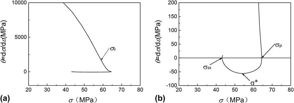
The work hardening rate curves can be obtained by the derivation of the fitting curves.^{Reference Najafizadeh and Jonas34}Figure 9 displays the work hardening rate (θ = dσ/dε) versus true stress (σ) curve at 980 °C and 0.001 s⁻¹.

FIG. 9.

Work hardening rate (θ = dσ/dε) versus true stress (σ) curve at 980 °C and 0.001 s⁻¹, (a) θ range from −2000 to 10,000; (b) θ range from −100 to 200.

In the first stage, the work hardening rate decreases rapidly and reaches an inflection point σ_c, which indicates the onset of DRX. As the hardening rate goes down to a point at which θ = 0, corresponding to the peak stress σ_p, the value of θ changes from positive to negative.^{Reference Ji, Li, Li, Li and Li33,Reference Quan, Wu, Luo, Xia, Zhou, Liu and Gao35} In the second stage, the curve keeps dropping and arrives at the lowest point σ*, while the related ε* indicates the maximum softening rate. In the third stage, the work hardening rate increases until the value of θ becomes 0 again, implying the steady-state flow of the initial σ–ε curve. In this way, the value of different parameters can be found in Table II.

Based on Eq. (11), Eq. (12), and the data in Table III, the constants n and k can be determined by linear fitting of the ln[−ln(1 − X _DRX)] to ln[(ε − ε_c)/ε*], and the slope and intercept are the n and ln k, respectively. Taking the condition of 980 °C, 0.001 s⁻¹ for example, the constant n and k are calculated as 2.50 and 0.77, as shown in Fig. 10(b). Therefore, the DRX kinetics model under this condition is:

$${X_{{\rm{DRX}}}} = 1 - \exp \left[ { - 0.77{{\left( {{{\varepsilon - 0.006747} \over {0.2986}}} \right)}^{2.5}}} \right]\quad .$$

TABLE III.

Values of different parameters.

FIG. 10.

(a) Nonlinear fitting for stress–strain curve and (b) linear fitting for ln[−ln(1 − X _DRX)]–ln[(ε − ε_c)/ε*] at 980 °C and 0.001 s⁻¹.

By applying the same method, all curves of DRX kinetics are shown in Fig. 11. At the beginning of the curve, the volume fraction of DRX grains remains at a relatively low level. It was also observed that the volume fraction of DRX grains increases as the strain increases and the evolution exhibits “slow-rapid-slow” growth trend in terms of S-curves, which has been also reported.^{Reference Liu, Cui and Ruan32}

FIG. 11.

The curves of DRX kinetics on conditions of (a) 980 °C, (b) 1030 °C, (c) 1080 °C and (d) ε = 0.001 s⁻¹.

Furthermore, it can be found that at high temperatures and high strain rates the DRX volume fraction tend to increase at a given strain, since the decrease in strain rate and the increase in temperature would facilitate the mobility of grain boundaries. However, the limit DRX behaviors of some specimens does not accord with the law, showing lower fraction at a given strain. This is because some experimental errors and nonuniformity of component in those samples. The process map (see Fig. 4) shows that all exceptions are in instability regions, revealing that the power dissipation (η) is consistent with the DRX evolution speed. More specifically, the low power dissipation usually contributes to a slow DRX evolution process despite the high temperature and the low strain rate.