1 Introduction
Stemming from early studies of the quantum Hall effect, Avron (Reference Avron1998) showed that apart from the well-known coefficient of viscosity, a classical liquid with broken time-reversal symmetry, either spontaneously or due to an external magnetic field or rotation, is endowed with a second viscosity coefficient termed odd or Hall viscosity. Such arguments had been put forward in the past in the context of plasmas (Lifshitz & Pitaevskii Reference Lifshitz and Pitaevskii1981) but only during the last few years have they received attention in the context of swimming strategies (Lapa & Hughes Reference Lapa and Hughes2014), chiral active liquids (Banerjee et al. Reference Banerjee, Souslov, Abanov and Vitelli2017) and the study of observable effects in incompressible liquids (Ganeshan & Abanov Reference Ganeshan and Abanov2017). Chiral surface waves satisfying a complex Burgers’ equation with imaginary viscosity have been found to exist even in the absence of gravity in such a liquid (Abanov, Can & Ganeshan Reference Abanov, Can and Ganeshan2018).
There are many instances in nature where the time-reversal symmetry of a classical liquid is broken, for instance in biological (Sumino et al. Reference Sumino, Nagai, Shitaka, Tanaka, Yoshikawa, Chaté and Oiwa2012), colloidal (Maggi et al. Reference Maggi, Saglimbeni, Dipalo, De Angelis and Di Leonardo2015) and granular systems (Tsai et al. Reference Tsai, Ye, Rodriguez, Gollub and Lubensky2005), and this new behaviour is expected to play a significant role in the dynamics of such systems, cf. Banerjee et al. (Reference Banerjee, Souslov, Abanov and Vitelli2017) and references therein. In addition, there are experimental observations in magnetic liquids (Chaves, Zahn & Rinaldi Reference Chaves, Zahn and Rinaldi2008) that cannot be explained by employing the classical theory of fluid flows. One such instance is the observation of interface patterns propagating in a direction opposite to the bulk liquid. Since time reversal is broken in such a system, it is expected that odd viscosity would play an important role.
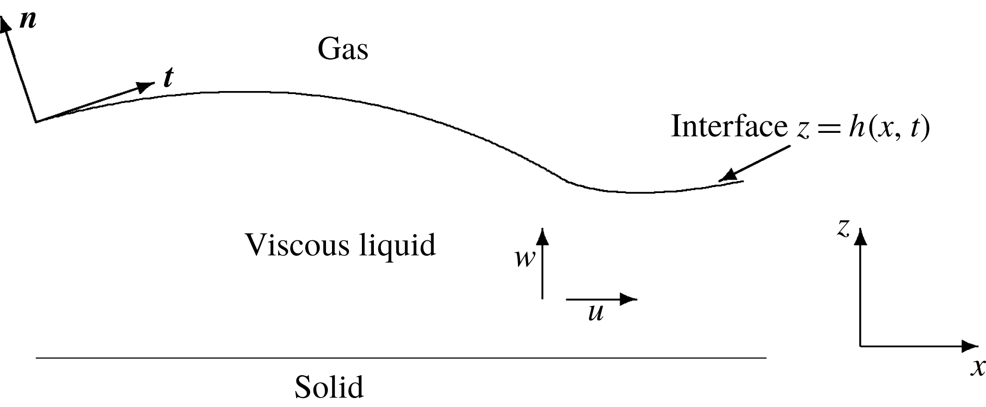
Geometry of the problem: a free interface at
 $z=h(x,t)$
with unit normal and tangent vectors
 $\boldsymbol{n}$
and
 $\boldsymbol{t}$
respectively, separates a gas phase from a viscous liquid (containing both even
 $\unicode[STIX]{x1D702}^{e}$
and odd
 $\unicode[STIX]{x1D702}^{o}$
viscosity coefficients) lying on a solid substrate. Here
 $u$
and
 $w$
are horizontal and vertical liquid velocities respectively. Dimensional quantities are denoted with lower case symbols here.

In this article we consider a classical Newtonian liquid with broken time-reversal symmetry and an odd or Hall viscosity coefficient. We envision that this effect is caused by the presence of an external magnetic field which is for example applied radially in a cylinder of a liquid with a free surface. Then, the Cauchy stress tensor, apart from the rate-of-strain tensor, acquires additional terms that depend on field direction which break the time-reversal symmetry (Lifshitz & Pitaevskii Reference Lifshitz and Pitaevskii1981, § 13). By reducing the problem’s geometry to two dimensions (see figure 1), thus considering the liquid sitting on a solid substrate and surrounded by an ambient gas phase in which the magnetic field is normal to the plane, we show that these new terms give rise to nonlinear viscous capillary waves that may lead to stabilization of an unstable film. We consider a thermocapillary system and show that odd viscosity can suppress the thermocapillary instability. These waves become prominent only when the shear surface stresses are spatially dependent. Two cases are developed in this article: surface stresses that arise due to the spatial variation of the surface tension (Oron, Davis & Bankoff Reference Oron, Davis and Bankoff1997; Davis Reference Davis, Batchelor, Moffatt and Worster2002) and surface shear that may arise from other sources such as blowing air (Davis, Gratton & Davis Reference Davis, Gratton and Davis2010) or applying a suitable temperature gradient (Kataoka & Troian Reference Kataoka and Troian1999).
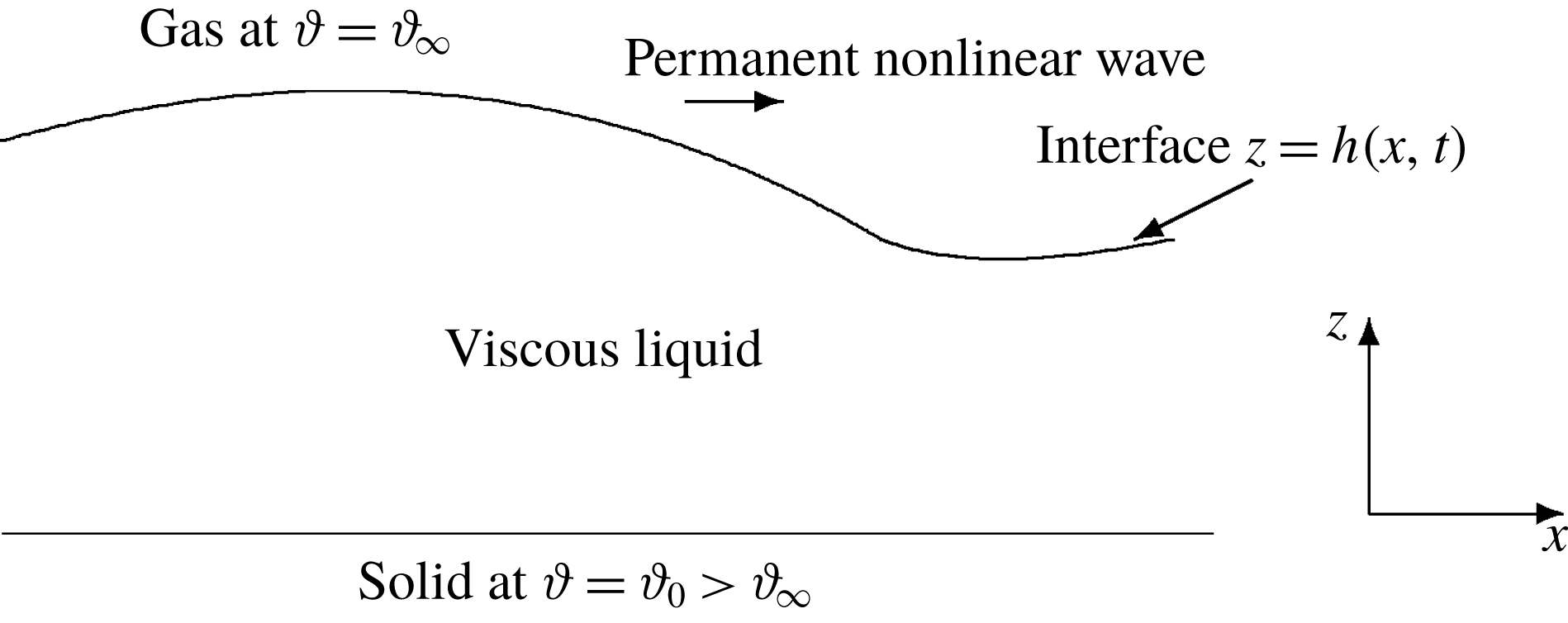
The thermocapillary effect: a free interface
 $z=h(x,t)$
separates a gas phase at temperature
 $\unicode[STIX]{x1D717}=\unicode[STIX]{x1D717}_{\infty }$
from a viscous liquid (containing both even
 $\unicode[STIX]{x1D702}^{e}$
and odd
 $\unicode[STIX]{x1D702}^{o}$
viscosity coefficients) lying on a solid substrate at temperature
 $\unicode[STIX]{x1D717}=\unicode[STIX]{x1D717}_{0}>\unicode[STIX]{x1D717}_{\infty }$
. Interfacial stresses arising from surface tension gradients, which in turn arise due to the temperature gradient, drive fluid from the hot depressions to the cool peaks leading to instability. The odd viscosity will give rise to wave propagation which, under certain circumstances, may lead to stabilization.

In § 2 we develop the theory of odd viscosity in the context of viscous thin liquid films by reducing the Navier–Stokes equations to a single partial differential equation describing the evolution of the liquid–gas interface. This reduction is possible by taking into account the long-wavelength approximation and retaining only the leading-order corrections (the lubrication approximation). Odd viscosity does not alter the shear stress but affects its normal counterpart at the free interface, in agreement with recent literature (Avron Reference Avron1998; Lapa & Hughes Reference Lapa and Hughes2014) where, for instance, a rotating disk experiences an additional pressure due to odd viscosity.
As a particular example in § 3 we employ a thermocapillary system (see figure 2) where interfacial shear stresses arise due to the variation of the surface tension
 $\unicode[STIX]{x1D70E}$
with temperature
 $\unicode[STIX]{x1D717}$
. If this variation is represented by a linear law
 $\unicode[STIX]{x1D70E}-\unicode[STIX]{x1D70E}_{0}\propto -(\unicode[STIX]{x1D717}-\unicode[STIX]{x1D717}_{0})$
valid for common liquids (the subscript denotes reference values), then there is a surface flow from the hot to the cold end. Since bulk fluids are viscous they are dragged along; thus, interfacial temperature gradients induce bulk-liquid motion. This is the thermocapillary effect (Davis Reference Davis1987; Oron et al.
Reference Oron, Davis and Bankoff1997; Davis Reference Davis, Batchelor, Moffatt and Worster2002). In the presence of odd viscosity, this effect gives rise to spatially dependent shear stresses at the liquid–gas interface which in turn enter the pressure gradient and generate nonlinear non-dissipative capillary waves. These waves act in a stabilizing manner: the thermocapillary instability is suppressed and an interfacial pattern persists. We numerically solve the evolution equation to show the existence of these waves.
In § 4.1 a linear stability analysis leads to the dispersion relation for the waves whereby the odd-viscosity contribution is cubic with respect to the wavenumber. Analogous behaviour has been discussed before in the context of soliton dynamics of dispersive nature similar to the Kuramoto–Sivashinsky equation (Kawahara Reference Kawahara1983; Kawahara & Toh Reference Kawahara and Toh1988).
In § 5 we develop a mean-field theory to explain the reason behind the appearance of these waves. Solutions of the evolution equation of the liquid–gas interface are invariant with respect to the
 $O(2)$
symmetry group of translations and reflections when odd viscosity vanishes (
 $\unicode[STIX]{x1D702}^{o}\equiv 0$
). A non-zero value of odd viscosity
 $\unicode[STIX]{x1D702}^{o}$
on the other hand, breaks the
 $O(2)$
reflection symmetry and endows these systems with an
 $SO(2)$
symmetry such that solutions become invariant with respect to parallel translations only. This broken symmetry induces patterns that slowly drift in the frame of reference moving with velocity
 $\unicode[STIX]{x1D702}^{o}$
. We perform a weakly nonlinear analysis of the evolution equation for an arbitrary value of the viscosity coefficient
 $\unicode[STIX]{x1D702}^{o}$
to determine the velocity of the patterns and investigate the stability of the Hopf bifurcation. We establish the conditions under which odd viscosity gives rise to stabilization of an unstable film.
The presence of the magnetic field endows the heat flux with additional terms that depend on the temperature gradient and the field direction (Lifshitz & Pitaevskii Reference Lifshitz and Pitaevskii1981, § 13). However, for a sufficiently thin film where the long-wavelength approximation can be taken into account we show that the balance of energy reduces to well-known expressions found in the literature (Oron et al. Reference Oron, Davis and Bankoff1997; Davis Reference Davis, Batchelor, Moffatt and Worster2002). We include such a discussion in appendix A. In addition, by resorting to the full energy equation of a liquid we show that viscous heating arises only as a consequence of even viscosity and odd viscosity plays no role in the evolution of the entropy of the system, see appendix B. In appendix C we derive the Landau equation for a thermocapillary system with odd viscosity. This result verifies the findings of the mean-field theory developed in § 5.
2 Odd viscosity in free surface viscous flows
Consider a two-dimensional thin liquid film (see figure 1) of thickness
 $h(x,t)$
sitting on a solid substrate surrounded by an ambient gas phase. In a liquid with broken time-reversal symmetry the Cauchy stress tensor
 $\unicode[STIX]{x1D748}$
consists of two parts:
 $$\begin{eqnarray}\unicode[STIX]{x1D748}=\unicode[STIX]{x1D748}^{e}+\unicode[STIX]{x1D748}^{o}.\end{eqnarray}$$
In two dimensions
 $$\begin{eqnarray}\unicode[STIX]{x1D70E}_{ik}^{e}=-p\unicode[STIX]{x1D6FF}_{ik}+\unicode[STIX]{x1D702}^{e}\left(\frac{\unicode[STIX]{x2202}u_{i}}{\unicode[STIX]{x2202}x_{k}}+\frac{\unicode[STIX]{x2202}u_{k}}{\unicode[STIX]{x2202}x_{i}}\right),\quad i,k=1,3,\end{eqnarray}$$
is the standard (even) Cauchy stress tensor with standard (even) viscosity
 $\unicode[STIX]{x1D702}^{e}$
and
 $\unicode[STIX]{x1D748}^{o}$
is the odd part of the Cauchy stress tensor which arises in the presence of time-reversal symmetry-breaking due, for instance, to a magnetic field. The general form of the odd stress tensor is characterized by several odd viscosity coefficients and depends on the orientation of the magnetic field (Lifshitz & Pitaevskii Reference Lifshitz and Pitaevskii1981, § 13), see also appendix A. We consider a planar flow in the
 $x$
–
 $z$
plane and assume that the magnetic field is perpendicular to it. In this case the odd part of the Cauchy stress tensor is characterized by a single odd viscosity coefficient and its components read (Avron Reference Avron1998; Lapa & Hughes Reference Lapa and Hughes2014)
 $$\begin{eqnarray}\unicode[STIX]{x1D70E}_{ik}^{o}=-\unicode[STIX]{x1D702}^{o}(\unicode[STIX]{x1D6FF}_{i1}\unicode[STIX]{x1D6FF}_{k1}-\unicode[STIX]{x1D6FF}_{i3}\unicode[STIX]{x1D6FF}_{k3})\left(\frac{\unicode[STIX]{x2202}u_{1}}{\unicode[STIX]{x2202}x_{3}}+\frac{\unicode[STIX]{x2202}u_{3}}{\unicode[STIX]{x2202}x_{1}}\right)+\unicode[STIX]{x1D702}^{o}(\unicode[STIX]{x1D6FF}_{i1}\unicode[STIX]{x1D6FF}_{k3}+\unicode[STIX]{x1D6FF}_{i3}\unicode[STIX]{x1D6FF}_{k1})\left(\frac{\unicode[STIX]{x2202}u_{1}}{\unicode[STIX]{x2202}x_{1}}-\frac{\unicode[STIX]{x2202}u_{3}}{\unicode[STIX]{x2202}x_{3}}\right),\end{eqnarray}$$
for
 $i,k=1,3$
, or explicitly, letting
 $u_{1}=u$
and
 $u_{3}=w$
,
 $$\begin{eqnarray}\unicode[STIX]{x1D70E}_{13}^{o}=\unicode[STIX]{x1D70E}_{31}^{o}=\unicode[STIX]{x1D702}^{o}(\unicode[STIX]{x2202}_{x}u-\unicode[STIX]{x2202}_{z}w)\quad \text{and}\quad \unicode[STIX]{x1D70E}_{33}^{o}=-\unicode[STIX]{x1D70E}_{11}^{o}=\unicode[STIX]{x1D702}^{o}(\unicode[STIX]{x2202}_{x}w+\unicode[STIX]{x2202}_{z}u),\end{eqnarray}$$
and
 $\unicode[STIX]{x1D702}^{o}$
is the odd viscosity. We emphasize that in the presence of odd viscosity, the Cauchy stress tensor
 $\unicode[STIX]{x1D748}$
remains symmetric.
The Navier–Stokes equations become
 $$\begin{eqnarray}\displaystyle & \unicode[STIX]{x1D70C}[u_{t}+uu_{x}+wu_{z}]=-p_{x}+\unicode[STIX]{x1D702}^{e}(u_{xx}+u_{zz})-\unicode[STIX]{x1D702}^{o}(w_{xx}+w_{zz})-\unicode[STIX]{x1D719}_{x}, & \displaystyle\end{eqnarray}$$
 $$\begin{eqnarray}\displaystyle & \unicode[STIX]{x1D70C}[w_{t}+uw_{x}+ww_{z}]=-p_{z}+\unicode[STIX]{x1D702}^{e}(w_{xx}+w_{zz})+\unicode[STIX]{x1D702}^{o}(u_{xx}+u_{zz})-\unicode[STIX]{x1D719}_{z}, & \displaystyle\end{eqnarray}$$
where
 $\unicode[STIX]{x1D719}$
is a potential representing the effects of gravity, intermolecular forces or other fields.
At the liquid–gas interface
 $z=h(x,t)$
, the shear and normal stresses are respectively
 $$\begin{eqnarray}\boldsymbol{t}\unicode[STIX]{x1D748}\boldsymbol{n}=\frac{\unicode[STIX]{x2202}\unicode[STIX]{x1D70E}}{\unicode[STIX]{x2202}s}+\unicode[STIX]{x1D70F}_{0}\quad \text{and}\quad \boldsymbol{n}\unicode[STIX]{x1D748}\boldsymbol{n}=2\unicode[STIX]{x1D705}\unicode[STIX]{x1D70E}+\unicode[STIX]{x1D6F1},\quad \text{at}\quad z=h(x,t),\end{eqnarray}$$
where
 $\unicode[STIX]{x1D70E}$
is the (variable) surface tension,
 $s$
is arc length along the interface,
 $\unicode[STIX]{x1D705}$
the mean curvature of the surface,
 $\unicode[STIX]{x1D70F}_{0}$
is an external shear stress and
 $\unicode[STIX]{x1D6F1}$
an external normal stress on the boundary (Oron et al.
Reference Oron, Davis and Bankoff1997).
No-slip and no-penetration boundary conditions at the liquid–solid interface are expressed as
 $$\begin{eqnarray}u=0\quad \text{and}\quad w=0,\quad \text{at}\quad z=0.\end{eqnarray}$$
The liquid–gas interface is described by the function
 $z=h(x,t)$
or, equivalently, the space curve
 $\boldsymbol{r}(x,t)=(x,h(x,t))$
. The tangent and normal vectors to the interface are
 $$\begin{eqnarray}\boldsymbol{t}=\frac{(1,h_{x})}{\sqrt{1+h_{x}^{2}}}\quad \text{and}\quad \boldsymbol{n}=\frac{(-h_{x},1)}{\sqrt{1+h_{x}^{2}}}.\end{eqnarray}$$
The shear and normal components of the stress tensor on the liquid–gas interface are respectively
 $$\begin{eqnarray}\boldsymbol{t}\unicode[STIX]{x1D748}\boldsymbol{n}=\frac{1}{1+h_{x}^{2}}(1,h_{x})\left(\begin{array}{@{}cc@{}}\unicode[STIX]{x1D70E}_{11} & \unicode[STIX]{x1D70E}_{13}\\ \unicode[STIX]{x1D70E}_{31} & \unicode[STIX]{x1D70E}_{33}\end{array}\right)\left(\begin{array}{@{}c@{}}-h_{x}\\ 1\end{array}\right)=\frac{1}{1+h_{x}^{2}}[\unicode[STIX]{x1D70E}_{13}-h_{x}^{2}\unicode[STIX]{x1D70E}_{31}+h_{x}(\unicode[STIX]{x1D70E}_{33}-\unicode[STIX]{x1D70E}_{11})]\end{eqnarray}$$
and
 $$\begin{eqnarray}\boldsymbol{n}\unicode[STIX]{x1D748}\boldsymbol{n}=\frac{1}{1+h_{x}^{2}}(-h_{x},1)\left(\begin{array}{@{}cc@{}}\unicode[STIX]{x1D70E}_{11} & \unicode[STIX]{x1D70E}_{13}\\ \unicode[STIX]{x1D70E}_{31} & \unicode[STIX]{x1D70E}_{33}\end{array}\right)\left(\begin{array}{@{}c@{}}-h_{x}\\ 1\end{array}\right)=\frac{1}{1+h_{x}^{2}}[\unicode[STIX]{x1D70E}_{33}+h_{x}^{2}\unicode[STIX]{x1D70E}_{11}-h_{x}(\unicode[STIX]{x1D70E}_{13}+\unicode[STIX]{x1D70E}_{31})],\end{eqnarray}$$
so that
 $$\begin{eqnarray}\frac{1}{1+h_{x}^{2}}[\unicode[STIX]{x1D70E}_{13}-h_{x}^{2}\unicode[STIX]{x1D70E}_{31}+h_{x}(\unicode[STIX]{x1D70E}_{33}-\unicode[STIX]{x1D70E}_{11})]=\frac{\unicode[STIX]{x2202}\unicode[STIX]{x1D70E}}{\unicode[STIX]{x2202}s}+\unicode[STIX]{x1D70F}_{0}\end{eqnarray}$$
and
 $$\begin{eqnarray}\frac{1}{1+h_{x}^{2}}[\unicode[STIX]{x1D70E}_{33}+h_{x}^{2}\unicode[STIX]{x1D70E}_{11}-h_{x}(\unicode[STIX]{x1D70E}_{13}+\unicode[STIX]{x1D70E}_{31})]=2\unicode[STIX]{x1D705}\unicode[STIX]{x1D70E}+\unicode[STIX]{x1D6F1},\end{eqnarray}$$
at the liquid–gas interface
 $z=h(x,t)$
. Equation (2.12) is the shear stress condition and (2.13) the Laplace condition of normal stress balance at the liquid–gas interface. Also,
 $2\unicode[STIX]{x1D705}=h_{xx}/(1+h_{x})^{3/2}$
. To the above one may add the kinematic condition
 $$\begin{eqnarray}w=h_{t}+uh_{x},\end{eqnarray}$$
at the liquid–gas interface.
Considering first the even-viscosity contributions we have (Oron et al. Reference Oron, Davis and Bankoff1997; Davis Reference Davis, Batchelor, Moffatt and Worster2002)
 $$\begin{eqnarray}\boldsymbol{t}\unicode[STIX]{x1D748}^{e}\boldsymbol{n}=\frac{1}{1+h_{x}^{2}}\unicode[STIX]{x1D702}^{e}[(-u_{x}+w_{z})h_{x}+\unicode[STIX]{x1D702}^{e}(1-h_{x}^{2})(w_{x}+u_{z})]\end{eqnarray}$$
and
 $$\begin{eqnarray}\boldsymbol{n}\unicode[STIX]{x1D748}^{e}\boldsymbol{n}=\frac{1}{1+h_{x}^{2}}[-p+2\unicode[STIX]{x1D702}^{e}w_{z}-2\unicode[STIX]{x1D702}^{e}h_{x}(w_{x}+u_{z})+h_{x}^{2}(-p+2\unicode[STIX]{x1D702}^{e}u_{x})].\end{eqnarray}$$
On the other hand, the contribution of the odd viscosity to the shear and normal stress is
 $$\begin{eqnarray}\boldsymbol{t}\unicode[STIX]{x1D748}^{o}\boldsymbol{n}=\frac{1}{1+h_{x}^{2}}\unicode[STIX]{x1D702}^{o}[(u_{x}-w_{z})(1-h_{x}^{2})+2h_{x}(w_{x}+u_{z})]\end{eqnarray}$$
and
 $$\begin{eqnarray}\boldsymbol{n}\unicode[STIX]{x1D748}^{o}\boldsymbol{n}=\frac{1}{1+h_{x}^{2}}\unicode[STIX]{x1D702}^{o}[(w_{x}+u_{z})(1-h_{x}^{2})-2h_{x}(u_{x}-w_{z})],\end{eqnarray}$$
respectively.
2.1 Lubrication approximation
In this approximation the Navier–Stokes equations are scaled with respect to a long wavelength
 $\unicode[STIX]{x1D706}$
which is a natural consequence of the longitudinal and vertical disparity of scales embodied in a thin liquid film. This introduces slow longitudinal and temporal variables
 $$\begin{eqnarray}X=\frac{2\unicode[STIX]{x03C0}x}{\unicode[STIX]{x1D706}}=\unicode[STIX]{x1D716}\frac{x}{h_{0}},\quad Z=\frac{z}{h_{0}}\quad \text{and}\quad T=\frac{2\unicode[STIX]{x03C0}U_{0}}{\unicode[STIX]{x1D706}}t,\quad \text{for}\quad \unicode[STIX]{x1D716}=\frac{2\unicode[STIX]{x03C0}h_{0}}{\unicode[STIX]{x1D706}},\end{eqnarray}$$
where
 $h_{0}$
and
 $U_{0}$
are characteristic scales for the liquid-film thickness and longitudinal velocity respectively and the partial derivatives
 $\unicode[STIX]{x2202}/\unicode[STIX]{x2202}X$
and
 $\unicode[STIX]{x2202}/\unicode[STIX]{x2202}Z$
are now quantities of unit order (Davis Reference Davis, Batchelor, Moffatt and Worster2002). The velocity, pressure and liquid–gas interface location become respectively
 $$\begin{eqnarray}U=\frac{u}{U_{0}},\quad W=\frac{\unicode[STIX]{x1D706}}{2\unicode[STIX]{x03C0}h_{0}}\frac{w}{U_{0}}=\frac{1}{\unicode[STIX]{x1D716}}\frac{w}{U_{0}},\quad P=\frac{2\unicode[STIX]{x03C0}h_{0}}{\unicode[STIX]{x1D706}}\frac{h_{0}p}{\unicode[STIX]{x1D702}^{e}U_{0}},\quad H=\frac{h}{h_{0}}.\end{eqnarray}$$
We define the dimensionless Reynolds and scaled capillary numbers and potential:
 $$\begin{eqnarray}Re=\frac{U_{0}h_{0}\unicode[STIX]{x1D70C}}{\unicode[STIX]{x1D702}^{e}},\quad \bar{C}=\unicode[STIX]{x1D716}^{-3}\frac{U_{0}\unicode[STIX]{x1D702}^{e}}{\unicode[STIX]{x1D70E}},\quad \unicode[STIX]{x1D6F7}=\frac{\unicode[STIX]{x1D716}h_{0}\unicode[STIX]{x1D719}}{\unicode[STIX]{x1D702}^{e}U_{0}}.\end{eqnarray}$$
With the above notation, equations (2.5) and (2.6) obtain the following dimensionless form:
 $$\begin{eqnarray}\displaystyle & \displaystyle \unicode[STIX]{x1D716}\,Re\frac{\text{D}U}{\text{D}T}=-P_{X}+(\unicode[STIX]{x1D716}^{2}U_{XX}+U_{ZZ})-\frac{\unicode[STIX]{x1D702}^{o}}{\unicode[STIX]{x1D702}^{e}}\unicode[STIX]{x1D716}(\unicode[STIX]{x1D716}^{2}W_{XX}+W_{ZZ})-\unicode[STIX]{x1D6F7}_{X}, & \displaystyle\end{eqnarray}$$
 $$\begin{eqnarray}\displaystyle & \displaystyle \unicode[STIX]{x1D716}^{2}Re\frac{\text{D}W}{\text{D}T}=-\frac{P_{Z}}{\unicode[STIX]{x1D716}}+\unicode[STIX]{x1D716}(\unicode[STIX]{x1D716}^{2}W_{XX}+W_{ZZ})+\frac{\unicode[STIX]{x1D702}^{o}}{\unicode[STIX]{x1D702}^{e}}(\unicode[STIX]{x1D716}^{2}U_{XX}+U_{ZZ})-\frac{1}{\unicode[STIX]{x1D716}}\unicode[STIX]{x1D6F7}_{Z}, & \displaystyle\end{eqnarray}$$
where
 $\text{D}U/\text{D}T=U_{T}+UU_{X}+WU_{Z}$
and
 $\text{D}W/\text{D}T=W_{T}+UW_{X}+WW_{Z}$
.
The shear and normal components of the stress tensor from relations (2.15)–(2.18) become
 $$\begin{eqnarray}\displaystyle & \displaystyle \boldsymbol{t}\unicode[STIX]{x1D748}^{e}\boldsymbol{n}=\frac{\unicode[STIX]{x1D702}^{e}U_{0}}{h_{0}}\frac{1}{1+\unicode[STIX]{x1D716}^{2}H_{X}^{2}}[\unicode[STIX]{x1D716}(-U_{X}+W_{Z})\unicode[STIX]{x1D716}H_{X}(1-\unicode[STIX]{x1D716}^{2}H_{X}^{2})(\unicode[STIX]{x1D716}^{2}W_{X}+U_{Z})], & \displaystyle\end{eqnarray}$$
 $$\begin{eqnarray}\displaystyle & \displaystyle \boldsymbol{n}\unicode[STIX]{x1D748}^{e}\boldsymbol{n}=\frac{1}{1\!+\unicode[STIX]{x1D716}^{2}H_{X}^{2}}\left[-p+2\unicode[STIX]{x1D702}^{e}\frac{\unicode[STIX]{x1D716}U_{0}}{h_{0}}W_{Z}-2\frac{\unicode[STIX]{x1D716}U_{0}}{h_{0}}\unicode[STIX]{x1D702}^{e}H_{X}(U_{Z}-\unicode[STIX]{x1D716}^{2}W_{X})\!+\unicode[STIX]{x1D716}^{2}H_{X}^{2}\left(\!-p\!+2\unicode[STIX]{x1D702}^{e}\frac{\unicode[STIX]{x1D716}U_{0}}{h_{0}}\unicode[STIX]{x1D716}U_{X}\!\right)\right], & \displaystyle \nonumber\\ \displaystyle & & \displaystyle\end{eqnarray}$$
 $$\begin{eqnarray}\displaystyle & \displaystyle \boldsymbol{t}\unicode[STIX]{x1D748}^{o}\boldsymbol{n}=\frac{\unicode[STIX]{x1D702}^{o}U_{0}}{h_{0}}\frac{1}{1+\unicode[STIX]{x1D716}H_{X}^{2}}[\unicode[STIX]{x1D716}(U_{X}-W_{Z})(1-\unicode[STIX]{x1D716}H_{X}^{2})+2\unicode[STIX]{x1D716}H_{X}(\unicode[STIX]{x1D716}^{2}W_{X}+U_{Z})] & \displaystyle\end{eqnarray}$$
and
 $$\begin{eqnarray}\boldsymbol{n}\unicode[STIX]{x1D748}^{o}\boldsymbol{n}=\frac{\unicode[STIX]{x1D702}^{o}U_{0}}{h_{0}}\frac{1}{1+\unicode[STIX]{x1D716}H_{X}^{2}}[(\unicode[STIX]{x1D716}^{2}W_{X}+U_{Z})(1-\unicode[STIX]{x1D716}H_{X}^{2})-2\unicode[STIX]{x1D716}^{2}H_{X}(U_{X}-W_{Z})].\end{eqnarray}$$
The kinematic condition (2.14) becomes
 $W=H_{T}+UH_{X}$
and leads to the following evolution equation for the liquid–gas profile
 $H$
:
 $$\begin{eqnarray}H_{T}+\left[\int _{0}^{H}U\,\text{d}Z\right]_{X}=0.\end{eqnarray}$$
This is obtained in the standard way (Oron et al.
Reference Oron, Davis and Bankoff1997) by integrating the incompressibility condition
 $U_{X}+W_{Z}=0$
from
 $Z=0$
to
 $Z=H(X,T)$
, using (2.8b
) and integration by parts.
We proceed by expanding all fields in a regular perturbation expansion with respect to the small parameter
 $\unicode[STIX]{x1D716}$
:
 $(U,W,P)=(U^{0},W^{0},P^{0})+\unicode[STIX]{x1D716}(U^{1},W^{1},P^{1})+O(\unicode[STIX]{x1D716}^{2})$
. To leading order (which corresponds to the lubrication approximation) and dropping superscripts denoting order in
 $\unicode[STIX]{x1D716}$
, the scaled equations (2.22)–(2.23) simplify to
 $$\begin{eqnarray}-\unicode[STIX]{x1D6F7}_{X}-P_{X}+U_{ZZ}=0,\quad -P_{Z}-\unicode[STIX]{x1D6F7}_{Z}=0.\end{eqnarray}$$
The boundary conditions (2.8) become
 $$\begin{eqnarray}U=0,\quad W=0,\quad \text{at}\quad Z=0.\end{eqnarray}$$
Introducing the dimensionless surface shear and surface tension
 $$\begin{eqnarray}\unicode[STIX]{x1D70F}=\frac{h_{0}\unicode[STIX]{x1D70F}_{0}}{\unicode[STIX]{x1D702}^{e}U_{0}}\quad \text{and}\quad \unicode[STIX]{x1D6F4}=\frac{\unicode[STIX]{x1D716}\unicode[STIX]{x1D70E}}{\unicode[STIX]{x1D702}^{e}U_{0}},\end{eqnarray}$$
respectively, we obtain the expressions for the sought shear stress by employing (2.7a ) (through (2.24) and (2.26))
 $$\begin{eqnarray}U_{Z}=\unicode[STIX]{x1D70F}+\unicode[STIX]{x1D6F4}_{X}.\end{eqnarray}$$
Equation (2.32) is identical to the one found in the literature of thin liquid films when only even viscosity is present (Oron et al. Reference Oron, Davis and Bankoff1997).
From (2.7b ) (through (2.25) and (2.27)) the normal stress reads
 $$\begin{eqnarray}-P+\frac{\unicode[STIX]{x1D702}^{o}}{\unicode[STIX]{x1D702}^{e}}U_{Z}=\bar{C}^{-1}H_{XX},\end{eqnarray}$$
where for simplicity we have set the normal stress at the boundary
 $\unicode[STIX]{x1D6F1}\equiv 0$
. Equation (2.33) shows that the presence of odd viscosity leads to an extra term in the normal boundary condition proportional to the velocity gradient
 $U_{Z}$
. This is the expected behaviour since it is known from the literature (Avron Reference Avron1998; Lapa & Hughes Reference Lapa and Hughes2014) that the effect of odd viscosity on a rotating disk is to apply a normal pressure. We may define its reduced counterpart (Oron et al.
Reference Oron, Davis and Bankoff1997; Davis Reference Davis, Batchelor, Moffatt and Worster2002)
 $$\begin{eqnarray}\bar{P}=P+\unicode[STIX]{x1D6F7}=\unicode[STIX]{x1D6F7}|_{Z=H}+\frac{\unicode[STIX]{x1D702}^{o}}{\unicode[STIX]{x1D702}^{e}}U_{Z}|_{Z=H}-\bar{C}^{-1}H_{XX}.\end{eqnarray}$$
Integration of (2.29b ) and application of the normal stress boundary condition (2.34) leads to the velocity distribution in the long-wavelength approximation (cf. Oron et al. (Reference Oron, Davis and Bankoff1997) equation (2.26))
 $$\begin{eqnarray}U(X,Z,T)=(\unicode[STIX]{x1D70F}+\unicode[STIX]{x1D6F4}_{X})Z+\bar{P}_{X}\left({\textstyle \frac{1}{2}}Z^{2}-HZ\right),\end{eqnarray}$$
where (2.32) and (2.34) lead to
 $$\begin{eqnarray}\bar{P}_{X}=\unicode[STIX]{x1D6F7}_{X}|_{Z=H}+\frac{\unicode[STIX]{x1D702}^{o}}{\unicode[STIX]{x1D702}^{e}}(\unicode[STIX]{x1D70F}+\unicode[STIX]{x1D6F4}_{X})_{X}-\bar{C}^{-1}H_{XXX}.\end{eqnarray}$$
The sought evolution equation for the liquid–gas interface (2.28) with the velocity profile (2.35) and pressure gradient from (2.36) becomes
 $$\begin{eqnarray}H_{T}+\left[{\textstyle \frac{1}{2}}(\unicode[STIX]{x1D70F}+\unicode[STIX]{x1D6F4}_{X})H^{2}-{\textstyle \frac{1}{3}}\bar{P}_{X}H^{3}\right]_{X}=0.\end{eqnarray}$$
Thus a non-zero odd viscosity
 $\unicode[STIX]{x1D702}^{o}$
leads to new effects in the evolution of thin liquid films. For example, thermocapillary flow with surface tension gradient
 $\unicode[STIX]{x1D6F4}_{X}$
, in addition to the well-known thinning and rupture of a thin liquid film, also leads to nonlinear capillary wave propagation. This case is analysed in the following sections.
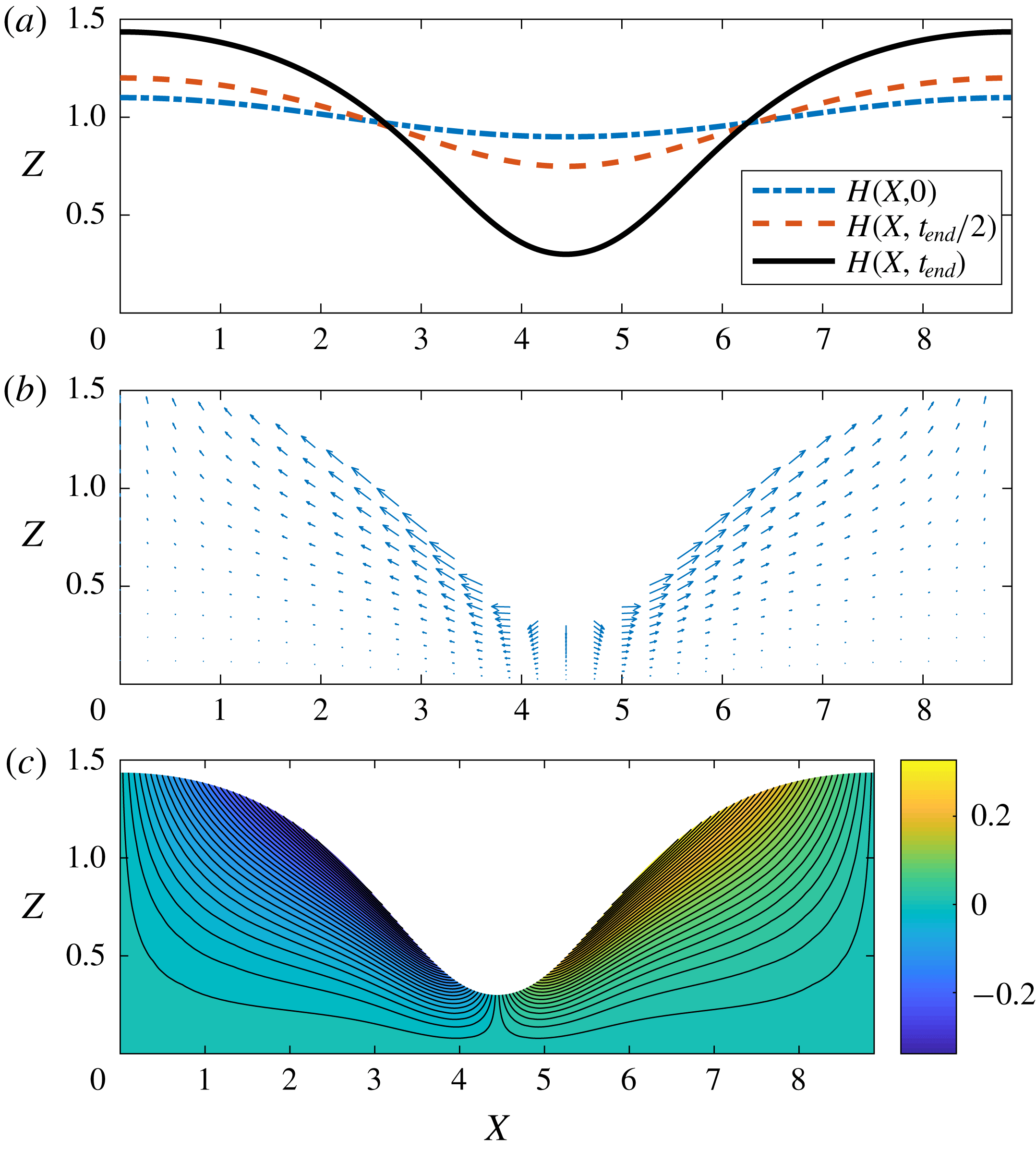
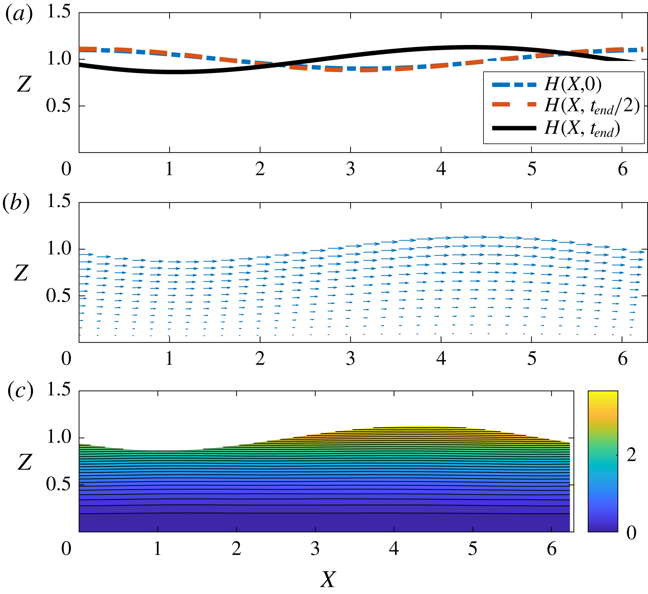
Surface tension gradients induced by temperature gradients lead to thinning of depressions in a thin liquid film without odd viscosity (
 $\unicode[STIX]{x1D702}^{o}=0$
). Numerical solutions of the thin-film equation (3.15) with surface tension gradient
 $\unicode[STIX]{x1D6F4}_{X}$
from (3.14). (a) Snapshots of the gas–liquid interface of a liquid film towards rupture. (b) Velocity field at time
 $t_{end}$
. (c) Streamlines at time
 $t_{end}$
.

3 Thermocapillary flow with odd viscosity
Consider a two-dimensional thin liquid film (cf. figure 2) of thickness
 $h(x,t)$
on a solid substrate surrounded by an ambient gas phase where interfacial shear stresses arise due to the variation of the surface tension
 $\unicode[STIX]{x1D70E}$
with temperature
 $\unicode[STIX]{x1D717}$
.
Thermocapillary instabilities arise because a corrugated interface in a fixed temperature gradient experiences hot regions at valleys and cool regions at peaks. The thermocapillary effect drives interfacial fluid from depressions to peaks and since the liquid is viscous, bulk fluid as well, see figure 3. This leads to film rupture and substrate dewetting (Oron et al. Reference Oron, Davis and Bankoff1997; Davis Reference Davis, Batchelor, Moffatt and Worster2002).
For an incompressible liquid the conservation of energy is given by (cf. Landau & Lifshitz (Reference Landau and Lifshitz1987) § 50)
 $$\begin{eqnarray}\unicode[STIX]{x1D70C}c_{p}(\unicode[STIX]{x1D717}_{t}+u\unicode[STIX]{x1D717}_{x}+w\unicode[STIX]{x1D717}_{z})=k_{th}\unicode[STIX]{x1D6FB}^{2}\unicode[STIX]{x1D717},\end{eqnarray}$$
where
 $c_{p}$
is the specific heat at constant pressure and
 $k_{th}$
is the thermal conductivity of the liquid.
The boundary conditions for a thermocapillary system are
 $$\begin{eqnarray}\unicode[STIX]{x1D717}=\unicode[STIX]{x1D717}_{0}\quad \text{at}\quad z=0\quad \text{and}\quad k_{th}\boldsymbol{n}\boldsymbol{\cdot }\unicode[STIX]{x1D735}\unicode[STIX]{x1D717}+\unicode[STIX]{x1D6FC}_{th}(\unicode[STIX]{x1D717}-\unicode[STIX]{x1D717}_{\infty })=0,\quad \text{at}\quad z=h(x,t),\end{eqnarray}$$
where
 $\unicode[STIX]{x1D717}_{0}$
is the temperature of the rigid plane,
 $\unicode[STIX]{x1D717}_{\infty }$
the temperature of the gas phase and
 $\unicode[STIX]{x1D6FC}_{th}$
the heat transfer coefficient describing the rate of heat transfer from the liquid to the ambient gas phase (Oron et al.
Reference Oron, Davis and Bankoff1997; Davis Reference Davis, Batchelor, Moffatt and Worster2002). We note that in the presence of a magnetic field the energy equation (3.1) and boundary conditions (3.2) are endowed with additional terms (see appendix A). In the long-wavelength approximation these terms are of higher order with respect to the perturbation parameter
 $\unicode[STIX]{x1D716}$
and they are not pursued further here. For certain system parameter regimes, viscous heating terms in (3.1) (Kirkinis & Andreev Reference Kirkinis and Andreev2019) may also become important. In this article we neglect such contributions as this is customary in the thin liquid film literature (Oron et al.
Reference Oron, Davis and Bankoff1997; Davis Reference Davis, Batchelor, Moffatt and Worster2002).
We now introduce the dimensionless temperature
 $$\begin{eqnarray}\unicode[STIX]{x1D6E9}(X,Z,T)=\frac{\unicode[STIX]{x1D717}-\unicode[STIX]{x1D717}_{\infty }}{\unicode[STIX]{x1D717}_{0}-\unicode[STIX]{x1D717}_{\infty }},\end{eqnarray}$$
as well as the dimensionless Prandtl and Biot numbers
 $$\begin{eqnarray}Pr=\frac{\unicode[STIX]{x1D702}^{e}c_{p}}{k_{th}},\quad B=\frac{\unicode[STIX]{x1D6FC}_{th}h_{0}}{k_{th}}.\end{eqnarray}$$
With these dimensionless quantities, the energy equation (3.1) and boundary conditions (3.2) become respectively (Oron et al. Reference Oron, Davis and Bankoff1997; Davis Reference Davis, Batchelor, Moffatt and Worster2002)
 $$\begin{eqnarray}\unicode[STIX]{x1D716}RePr(\unicode[STIX]{x1D6E9}_{T}+U\unicode[STIX]{x1D6E9}_{X}+W\unicode[STIX]{x1D6E9}_{Z})=\unicode[STIX]{x1D716}^{2}\unicode[STIX]{x1D6E9}_{XX}+\unicode[STIX]{x1D6E9}_{ZZ}\end{eqnarray}$$
and
 $$\begin{eqnarray}\unicode[STIX]{x1D6E9}=1\quad \text{at}\quad Z=0\quad \text{and}\quad \unicode[STIX]{x1D6E9}_{Z}-\unicode[STIX]{x1D716}^{2}\unicode[STIX]{x1D6E9}_{X}H_{X}+B\unicode[STIX]{x1D6E9}(1+\unicode[STIX]{x1D716}^{2}H_{X}^{2})^{1/2}=0\quad \text{at}\quad Z=H.\end{eqnarray}$$
Employing the long-wavelength approximation and considering the leading-order correction (the lubrication approximation), energy equation (3.5) and boundary conditions (3.6a,b ) become respectively
 $$\begin{eqnarray}\unicode[STIX]{x1D6E9}_{ZZ}=0\end{eqnarray}$$
and
 $$\begin{eqnarray}\unicode[STIX]{x1D6E9}=1\quad \text{at}\quad Z=0,\quad \unicode[STIX]{x1D6E9}_{Z}+B\unicode[STIX]{x1D6E9}=0\quad \text{at}\quad Z=H(X,T).\end{eqnarray}$$
Other dimensionless parameters employed in the subsequent analysis are the gravity number
 $G$
and the Marangoni number
 $M$
:
 $$\begin{eqnarray}G=\unicode[STIX]{x1D716}\frac{\unicode[STIX]{x1D70C}gh_{0}^{2}}{\unicode[STIX]{x1D702}^{e}U_{0}},\quad M=\frac{\unicode[STIX]{x0394}\unicode[STIX]{x1D70E}}{\unicode[STIX]{x1D702}^{e}U_{0}}\unicode[STIX]{x1D716},\end{eqnarray}$$
where
 $\unicode[STIX]{x0394}\unicode[STIX]{x1D70E}$
is the variation of surface tension over the temperature domain
 $\unicode[STIX]{x0394}\unicode[STIX]{x1D717}=\unicode[STIX]{x1D717}_{0}-\unicode[STIX]{x1D717}_{\infty }$
so that
 $$\begin{eqnarray}\unicode[STIX]{x0394}\unicode[STIX]{x1D70E}=\unicode[STIX]{x1D6FE}\unicode[STIX]{x0394}\unicode[STIX]{x1D703}.\end{eqnarray}$$
Equation (3.10) is derived from the equation of state approximated by a linear law
 $$\begin{eqnarray}\unicode[STIX]{x1D70E}=\unicode[STIX]{x1D70E}_{0}-\unicode[STIX]{x1D6FE}(\unicode[STIX]{x1D717}-\unicode[STIX]{x1D717}_{0}),\end{eqnarray}$$
where
 $\unicode[STIX]{x1D6FE}$
is positive for common liquids (Oron et al.
Reference Oron, Davis and Bankoff1997; Davis Reference Davis, Batchelor, Moffatt and Worster2002).
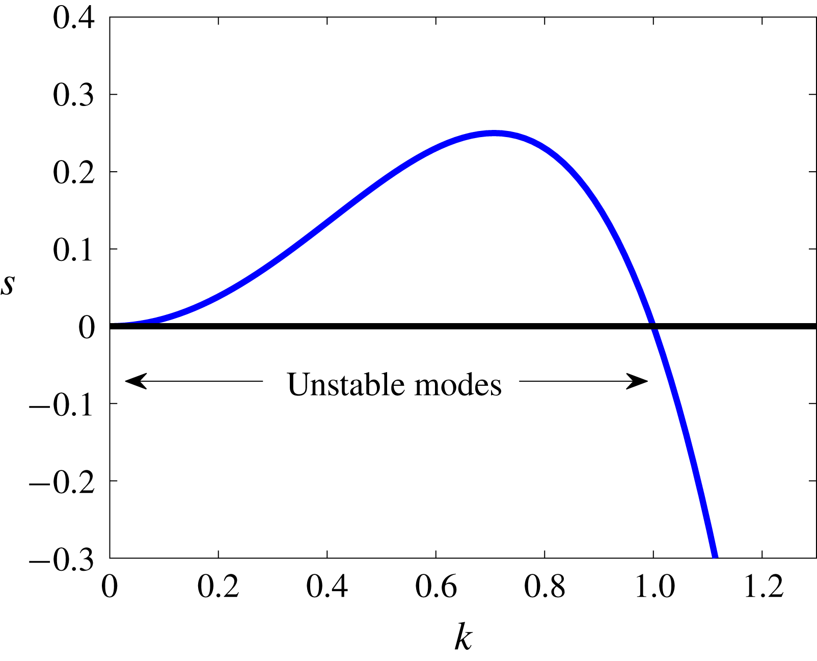
Growth rate
 $s=k^{2}-k^{4}$
obtained from linear stability analysis (Oron et al.
Reference Oron, Davis and Bankoff1997; Davis Reference Davis, Batchelor, Moffatt and Worster2002) of the thin-film evolution equation (3.15) showing the band of unstable wavenumbers
 $0<k<k_{cr}=1$
.

Equation (3.7) leads to the well-known form of the temperature distribution (Oron et al. Reference Oron, Davis and Bankoff1997; Davis Reference Davis, Batchelor, Moffatt and Worster2002)
 $$\begin{eqnarray}\unicode[STIX]{x1D6E9}(X,Z,T)=1-\frac{BZ}{1+BH}.\end{eqnarray}$$
3.1 Evolution equation for the liquid–gas interface
We thus need to calculate
 $\unicode[STIX]{x1D6F4}_{X}$
. This can be done by considering the variation of the surface tension at the liquid–gas interface, that is,
 $\unicode[STIX]{x1D6F4}=\unicode[STIX]{x1D6F4}(\unicode[STIX]{x1D6E9}(H))$
. The chain rule leads to
 $$\begin{eqnarray}\unicode[STIX]{x1D6F4}_{X}=\frac{\text{d}\unicode[STIX]{x1D6F4}}{\text{d}\unicode[STIX]{x1D6E9}}\left[\frac{\unicode[STIX]{x2202}\unicode[STIX]{x1D6E9}}{\unicode[STIX]{x2202}X}\right].\end{eqnarray}$$
As is common in the literature we set
 $\text{d}\unicode[STIX]{x1D6F4}/\text{d}\unicode[STIX]{x1D6E9}=-M$
, where
 $M$
is the Marangoni number. We thus obtain that
 $$\begin{eqnarray}\unicode[STIX]{x1D6F4}_{X}=\frac{BMH_{X}}{(1+BH)^{2}},\end{eqnarray}$$
which is the standard result obtained in the literature (Oron et al. Reference Oron, Davis and Bankoff1997; Davis Reference Davis, Batchelor, Moffatt and Worster2002). Thus, our aim is to solve the evolution equation (2.37) with the surface tension gradient given by (3.14), that is, solve
 $$\begin{eqnarray}H_{T}+\unicode[STIX]{x1D70F}HH_{X}+\left[\frac{1}{2}\unicode[STIX]{x1D6F4}_{X}H^{2}-\frac{1}{3}\left(\frac{\unicode[STIX]{x1D702}^{o}}{\unicode[STIX]{x1D702}^{e}}\unicode[STIX]{x1D6F4}_{XX}+GH_{X}-\bar{C}^{-1}H_{XXX}\right)H^{3}\right]_{X}=0.\end{eqnarray}$$
In the subsequent discussion we will consider a constant surface shear
 $\unicode[STIX]{x1D70F}$
so only the surface tension gradient will appear in the expression for the pressure.
4 Stability analysis
4.1 Linear stability
Following the standard linear stability analysis of Oron et al. (Reference Oron, Davis and Bankoff1997) and Davis (Reference Davis, Batchelor, Moffatt and Worster2002) by substituting
 $H=1+\unicode[STIX]{x1D6FF}\text{e}^{sT+\text{i}(kX-\unicode[STIX]{x1D714}T)}$
into (3.15) (assuming that
 $s$
and
 $\unicode[STIX]{x1D714}$
are real and
 $\unicode[STIX]{x1D6FF}\ll 1$
) we obtain the growth rate and frequency
 $$\begin{eqnarray}s=\left[\frac{MB}{2(1+B)^{2}}-\frac{G}{3}\right]k^{2}-\frac{1}{3\bar{C}}k^{4},\quad \unicode[STIX]{x1D714}=\unicode[STIX]{x1D70F}k+\frac{k^{3}}{3}\frac{\unicode[STIX]{x1D702}^{o}}{\unicode[STIX]{x1D702}^{e}}\frac{BM}{(1+B)^{2}},\end{eqnarray}$$
respectively. Thus, there is a band of unstable wavenumbers
 $0<k<k_{cr}$
whose critical value
 $k_{cr}$
for the onset of instability is found when
 $s$
becomes positive, that is, when
 $$\begin{eqnarray}k_{cr}^{2}=\frac{3MB\bar{C}}{2(1+B)^{2}}-\bar{C}G.\end{eqnarray}$$
This requires that the Marangoni number
 $M$
exceeds its critical value
 $$\begin{eqnarray}M_{cr}=\frac{2G(1+B)^{2}}{3B}.\end{eqnarray}$$
For values
 $M=4(1+B)^{2}/B,G=3,\bar{C}=1/3$
we obtain the critical wavenumber
 $k_{cr}=1$
and the band of unstable wavenumbers
 $0<k<1$
, see figure 4.
The wavenumber dependence of the frequency
 $\unicode[STIX]{x1D714}$
in (4.1) is suggestive of the effectiveness of odd viscosity in stabilizing a film. Because odd viscosity is associated with cubic terms of wavenumber it is expected that stabilization will take place only at high wavenumbers.
5 Travelling waves in odd-viscosity liquids
5.1
 $O(2)$
and
$SO(2)$
symmetries of the thin-film equations


In the absence of odd viscosity (
 $\unicode[STIX]{x1D702}^{o}\equiv 0$
) and surface shear (
 $\unicode[STIX]{x1D70F}\equiv 0$
) the thin-film equation (3.15) is invariant under the group
 $O(2)$
of parallel translations and reflections
 $$\begin{eqnarray}\unicode[STIX]{x1D6F1}_{1}:X\rightarrow X+X_{0},\quad \unicode[STIX]{x1D6F1}_{2}:X\rightarrow -X.\end{eqnarray}$$
If an external mechanism such as a magnetic field becomes operative, time-reversal breaks and odd viscosity becomes prominent. Non-vanishing odd viscosity or surface shear gives rise to a new term in the thin-film equation (3.15) (second or fourth term) that breaks the reflection (but not the parallel translation) symmetry. The surface shear term is of advective character and has been discussed before in the context of suppressing the van-der-Waals-driven rupture (Kirkinis & Davis Reference Kirkinis and Davis2015). The term associated with odd viscosity is of (nonlinearly) dispersive nature analogous to the dispersive Kuramoto–Sivashinsky equation (Kawahara Reference Kawahara1983; Kawahara & Toh Reference Kawahara and Toh1988).
5.2 Broken symmetry
At the threshold of instability, there is a subcritical pitchfork bifurcation, already discussed in the literature of thin liquid films (Erneux & Davis Reference Erneux and Davis1993). In this case the liquid–gas interface profile satisfying (3.15) has the form
 $$\begin{eqnarray}H(X,T)=1+\unicode[STIX]{x1D6FF}Re\{A(T)\text{e}^{\text{i}qX}\}+O(\unicode[STIX]{x1D6FF}^{2}),\end{eqnarray}$$
where
 $q$
is the critical wavenumber and
 $\unicode[STIX]{x1D6FF}$
measures distance from criticality. The absence of odd viscosity (
 $\unicode[STIX]{x1D702}^{o}\equiv 0$
) and surface shear (
 $\unicode[STIX]{x1D70F}\equiv 0$
) imparts the following properties onto the complex amplitude
 $A$
:
 $$\begin{eqnarray}\text{parallel translation}\quad \unicode[STIX]{x1D6F1}_{1}:X\rightarrow X+X_{0},\quad A\rightarrow A\text{e}^{\text{i}qX_{0}}\end{eqnarray}$$
and
 $$\begin{eqnarray}\text{reflection}\quad \unicode[STIX]{x1D6F1}_{2}:X\rightarrow -X,\quad A\rightarrow A^{\ast }.\end{eqnarray}$$
Thus, the amplitude equation is a Landau equation of the general form
 $$\begin{eqnarray}A_{T}=\unicode[STIX]{x1D6FC}_{1}A+\unicode[STIX]{x1D6FC}_{2}A|A|^{2},\end{eqnarray}$$
for some constants
 $\unicode[STIX]{x1D6FC}_{i}$
that in general depend on the wavenumber
 $q$
at the onset of instability. When
 $\unicode[STIX]{x1D6FC}_{2}>0$
the resulting equilibria correspond to a subcritical pitchfork (Cross & Hohenberg Reference Cross and Hohenberg1993, p. 867). In polar coordinates where
 $A=R\text{e}^{\text{i}\unicode[STIX]{x1D703}}$
(5.5) can be expressed as
 $R_{T}=\unicode[STIX]{x1D6FC}_{1}R+\unicode[STIX]{x1D6FC}_{2}R^{3}$
and
 $\unicode[STIX]{x1D703}_{T}=0.$
In the presence of odd viscosity or surface shear, either of the terms
 ${\textstyle \frac{1}{2}}[H^{2}\unicode[STIX]{x1D6F4}_{XX}]_{X}$
or
 $\unicode[STIX]{x1D70F}HH_{X}$
breaks the reflection symmetry of (3.15) and the Landau equation acquires complex coefficients
 $$\begin{eqnarray}A_{T}=(\unicode[STIX]{x1D6FC}_{1}+\text{i}\unicode[STIX]{x1D6FD}_{1}\unicode[STIX]{x1D702}^{o})A+(\unicode[STIX]{x1D6FC}_{2}+\text{i}\unicode[STIX]{x1D6FD}_{2}\unicode[STIX]{x1D702}^{o})A|A|^{2},\end{eqnarray}$$
for some constants
 $\unicode[STIX]{x1D6FC}_{i}$
and
 $\unicode[STIX]{x1D6FD}_{i}$
which, in general, depend on
 $\unicode[STIX]{x1D702}^{o}$
(or
 $\unicode[STIX]{x1D70F}$
). In polar coordinates the phase of (5.6) can be expressed as
 $\unicode[STIX]{x1D703}_{T}=\unicode[STIX]{x1D702}^{o}(\unicode[STIX]{x1D6FD}_{1}+\unicode[STIX]{x1D6FD}_{2}R^{2}).$
Now, the resulting equilibria correspond to a Hopf bifurcation which implies travelling wave solutions of the thin-film equation (3.15).
5.3 Mean-field analysis
We perform a mean-field analysis of (3.15) for an arbitrary value of the odd viscosity
 $\unicode[STIX]{x1D702}^{o}$
in the vicinity of the onset of instability following the arguments developed by Kirkinis & Davis (Reference Kirkinis and Davis2015). We introduce a Galilean frame of reference
 $\unicode[STIX]{x1D709}=X-VT$
moving with velocity
 $V$
. Substituting into (3.15) and performing one integration we obtain
 $$\begin{eqnarray}-VH+\frac{1}{2}(\unicode[STIX]{x1D70F}+\unicode[STIX]{x1D6F4}_{\unicode[STIX]{x1D709}})H^{2}-\frac{1}{3}\left(\frac{\unicode[STIX]{x1D702}^{o}}{\unicode[STIX]{x1D702}^{e}}\unicode[STIX]{x1D6F4}_{\unicode[STIX]{x1D709}\unicode[STIX]{x1D709}}+GH_{\unicode[STIX]{x1D709}}-\bar{C}^{-1}H_{\unicode[STIX]{x1D709}\unicode[STIX]{x1D709}\unicode[STIX]{x1D709}}\right)H^{3}=K,\end{eqnarray}$$
where
 $K$
is an integration constant.
We expand
 $K$
and
 $M$
in a perturbation series or equivalently
 $K$
and the bifurcation parameter
 $$\begin{eqnarray}a=\frac{M-M_{cr}}{M_{cr}},\end{eqnarray}$$
where
 $M_{cr}=(2/3)G(1+B)^{2}/B$
is the critical Marangoni number. Thus,
 $$\begin{eqnarray}(V,K,a)=(V_{0},K_{0},a_{0})+\unicode[STIX]{x1D6FF}(V_{1},K_{1},a_{1})+\unicode[STIX]{x1D6FF}^{2}(V_{2},K_{2},a_{2})+O(\unicode[STIX]{x1D6FF}^{3}),\end{eqnarray}$$
and expand
 $H$
about a steady state
 $$\begin{eqnarray}H=1+\unicode[STIX]{x1D6FF}(A_{c}\cos q\unicode[STIX]{x1D709}+A_{s}\sin q\unicode[STIX]{x1D709})+\unicode[STIX]{x1D6FF}^{2}(B_{c}\cos 2q\unicode[STIX]{x1D709}+B_{s}\sin 2q\unicode[STIX]{x1D709})+O(\unicode[STIX]{x1D6FF}^{2}),\end{eqnarray}$$
for real amplitudes
 $A_{c},B_{c}$
etc. and wavenumber
 $q$
associated with the primary bifurcation. Here
 $\unicode[STIX]{x1D6FF}$
denotes distance from criticality.
To leading order in
 $\unicode[STIX]{x1D6FF}$
we find
 $$\begin{eqnarray}V_{0}=\frac{2(\bar{C}G+q^{2})q^{2}}{9\bar{C}}\frac{\unicode[STIX]{x1D702}^{o}}{\unicode[STIX]{x1D702}^{e}}+\unicode[STIX]{x1D70F},\quad K_{0}=-V_{0}+\frac{\unicode[STIX]{x1D70F}}{2}\quad \text{and}\quad a_{0}=\frac{q^{2}}{\bar{C}G}.\end{eqnarray}$$
 $V_{0}$
and
 $a_{0}$
are the standard results of linear stability analysis (Oron et al.
Reference Oron, Davis and Bankoff1997). For instance,
 $V_{0}$
can be derived by substituting into
 $\unicode[STIX]{x1D714}$
(4.1) the Marangoni number from (4.2). The first-order corrections vanish and, to second order, we obtain
 $$\begin{eqnarray}\displaystyle a_{2} & = & \displaystyle -\frac{9({A_{c}}^{2}+{A_{s}}^{2})}{4\bar{C}\left((\bar{C}G+q^{2})^{2}\left({\displaystyle \frac{\unicode[STIX]{x1D702}^{o}}{\unicode[STIX]{x1D702}^{e}}}\right)^{2}+9q^{2}\right)G(B+1)^{2}}\nonumber\\ \displaystyle & & \displaystyle \times \left(\!\frac{1}{27}(\bar{C}G+q^{2})^{2}(27B^{2}\bar{C}G+35\,B^{2}q^{2}+42B\bar{C}G+30Bq^{2}+12\bar{C}G-24q^{2})\!\!\left(\frac{\unicode[STIX]{x1D702}^{o}}{\unicode[STIX]{x1D702}^{e}}\right)^{\!2}\right.\nonumber\\ \displaystyle & & \displaystyle +\,\frac{1}{12q^{2}}\bar{C}(B\,+\,1)(\bar{C}G\,+\,q^{2})(9B\bar{C}G\,+\,5Bq^{2}\,+\,3\bar{C}G\,-\,21q^{2})\unicode[STIX]{x1D70F}\frac{\unicode[STIX]{x1D702}^{o}}{\unicode[STIX]{x1D702}^{e}}\,-\,\frac{3}{4q^{2}}C^{2}\unicode[STIX]{x1D70F}^{2}(B+1)^{2}\nonumber\\ \displaystyle & & \displaystyle +\left.(\bar{C}G+q^{2})\left(\frac{3}{2}B^{2}\bar{C}G+B\bar{C}G+\frac{1}{6}\bar{C}G+\frac{15}{2}\,B^{2}q^{2}+5Bq^{2}+\frac{7}{6}q^{2}\right)\right),\end{eqnarray}$$
 $$\begin{eqnarray}\displaystyle V_{2} & = & \displaystyle -\frac{7({A_{c}}^{2}+{A_{s}}^{2})}{\left(27(\bar{C}G+q^{2})^{2}\left({\displaystyle \frac{\unicode[STIX]{x1D702}^{o}}{\unicode[STIX]{x1D702}^{e}}}\right)^{2}+243q^{2}\right)(B+1)^{2}\bar{C}}\nonumber\\ \displaystyle & & \displaystyle \times \left(\frac{1}{7}\,q^{2}(\bar{C}G+q^{2})^{2}(7\,B^{2}\bar{C}G+11\,B^{2}q^{2}+24\,B\bar{C}G+18\,Bq^{2}+15\,\bar{C}G-3\,q^{2})\right.\nonumber\\ \displaystyle & & \displaystyle \times \left(\frac{\unicode[STIX]{x1D702}^{o}}{\unicode[STIX]{x1D702}^{e}}\right)^{3}+\frac{9\,\bar{C}(B+1)q^{2}(\bar{C}G+q^{2})(5\,B\bar{C}G+4\,Bq^{2}+6\,\bar{C}G)\unicode[STIX]{x1D70F}}{14q^{2}}\left(\frac{\unicode[STIX]{x1D702}^{o}}{\unicode[STIX]{x1D702}^{e}}\right)^{2}\nonumber\\ \displaystyle & & \displaystyle +\,\frac{81\,\bar{C}^{2}(B+1)^{2}(\bar{C}G-q^{2})\unicode[STIX]{x1D70F}^{2}}{112q^{2}}\frac{\unicode[STIX]{x1D702}^{o}}{\unicode[STIX]{x1D702}^{e}}+\frac{243\,\bar{C}(B+1)q^{2}(3\,B\bar{C}G+9\,Bq^{2}+\bar{C}G+7\,q^{2})\unicode[STIX]{x1D70F}}{112q^{2}}\nonumber\\ \displaystyle & & \displaystyle -\left.\frac{(27\,B+9)(3\,B\bar{C}^{2}G^{2}-6\,B\bar{C}Gq^{2}-21\,Bq^{4}+\bar{C}^{2}G^{2}-18\,\bar{C}Gq^{2}-31\,q^{4})}{56}\frac{\unicode[STIX]{x1D702}^{o}}{\unicode[STIX]{x1D702}^{e}}\right)\nonumber\\ \displaystyle & & \displaystyle\end{eqnarray}$$
and
 $$\begin{eqnarray}K_{2}=-V_{2}+(A_{c}^{2}+A_{s}^{2})\left(\frac{(\bar{C}G+q^{2})q^{2}}{3\bar{C}}\frac{\unicode[STIX]{x1D702}^{o}}{\unicode[STIX]{x1D702}^{e}}+\frac{\unicode[STIX]{x1D70F}}{4}\right).\end{eqnarray}$$
We recognize the last term in (5.12) as being the well-known correction (see equation (2.27) in Kirkinis & Davis (Reference Kirkinis and Davis2015) by setting
 $\unicode[STIX]{x1D70F}=0$
) signifying the subcritical behaviour of the bifurcation, a subcritical pitchfork of revolution.
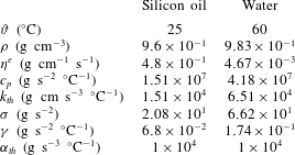
Experimental values taken from Tan, Bankoff & Davis (Reference Tan, Bankoff and Davis1990).

When
 $\unicode[STIX]{x1D702}^{o}=0$
(5.12) shows that there is a critical value
 $\unicode[STIX]{x1D70F}_{cr}$
of the surface shear above which the Hopf bifurcation becomes supercritical
 $$\begin{eqnarray}\unicode[STIX]{x1D70F}_{cr}^{2}=\frac{2q^{2}(\bar{C}G+q^{2})(9\,B^{2}\bar{C}G+45\,B^{2}q^{2}+6\,B\bar{C}G+30\,Bq^{2}+\bar{C}G+7\,q^{2})}{9(B+1)^{2}\bar{C}^{2}}.\end{eqnarray}$$
Similarly, when
 $\unicode[STIX]{x1D70F}=0$
(5.12) shows that there is a critical value of odd viscosity
 $\unicode[STIX]{x1D702}_{cr}^{o}$
 $$\begin{eqnarray}\left(\frac{\unicode[STIX]{x1D702}^{o}}{\unicode[STIX]{x1D702}^{e}}\right)_{cr}^{2}=\frac{-9(9\,B^{2}\bar{C}G+45\,B^{2}q^{2}+6\,B\bar{C}G+30\,Bq^{2}+\bar{C}G+7\,q^{2})}{2(\bar{C}G+q^{2})(27\,B^{2}\bar{C}G+35\,B^{2}q^{2}+42\,B\bar{C}G+30\,Bq^{2}+12\,\bar{C}G-24\,q^{2})},\end{eqnarray}$$
as long as the denominator in (5.16) is negative. This is ensured when
 $$\begin{eqnarray}q^{2}>-3\,\frac{\bar{C}G(9\,B^{2}+14\,B+4)}{35\,B^{2}+30\,B-24},\end{eqnarray}$$
which in turn sets an upper bound on the Biot number
 $B$
 $$\begin{eqnarray}B<-\frac{3}{7}+\frac{\sqrt{1065}}{35}\sim 0.5.\end{eqnarray}$$
This bound is consistent with the behaviour of common liquids (Oron et al.
Reference Oron, Davis and Bankoff1997). In the limit of small Biot number
 $B\rightarrow 0$
we require that
 $$\begin{eqnarray}q^{2}>\frac{\bar{C}G}{2}.\end{eqnarray}$$
As expected then, from our discussion in § 4.1, only high-wavenumber perturbations to the free surface can be stabilized with odd viscosity.
The following three parameter regimes can be distinguished.
(i) When
$(\unicode[STIX]{x1D70F},\unicode[STIX]{x1D702}^{o})=(0,0)$
,
$a_{2}$
is always negative (see the last term in (5.12)) and the film is unstable; it proceeds to rupture and leads to substrate dewetting. This corresponds to a subcritical bifurcation. This behaviour corresponds to the film snapshots in figure 3(a).(ii) When
$\unicode[STIX]{x1D702}^{o}=0$
and
$0<\unicode[STIX]{x1D70F}<\unicode[STIX]{x1D70F}_{cr}$
or when
$\unicode[STIX]{x1D70F}=0$
and
$0<\unicode[STIX]{x1D702}^{o}<\unicode[STIX]{x1D702}_{cr}^{o}$
subject to the condition (5.19), there is wave propagation but the film still ruptures albeit at a reduced rate;
$a_{2}$
is still negative but approaches its zero value. The bifurcation is a subcrtitical Hopf.(iii) When
$\unicode[STIX]{x1D702}^{o}=0$
and
$\unicode[STIX]{x1D70F}>\unicode[STIX]{x1D70F}_{cr}$
or when
$\unicode[STIX]{x1D70F}=0$
and
$\unicode[STIX]{x1D702}>\unicode[STIX]{x1D702}_{cr}^{o}$
subject to the condition (5.19) there is wave propagation and the film reaches a stable steady state in the frame of reference moving with velocity
$V$
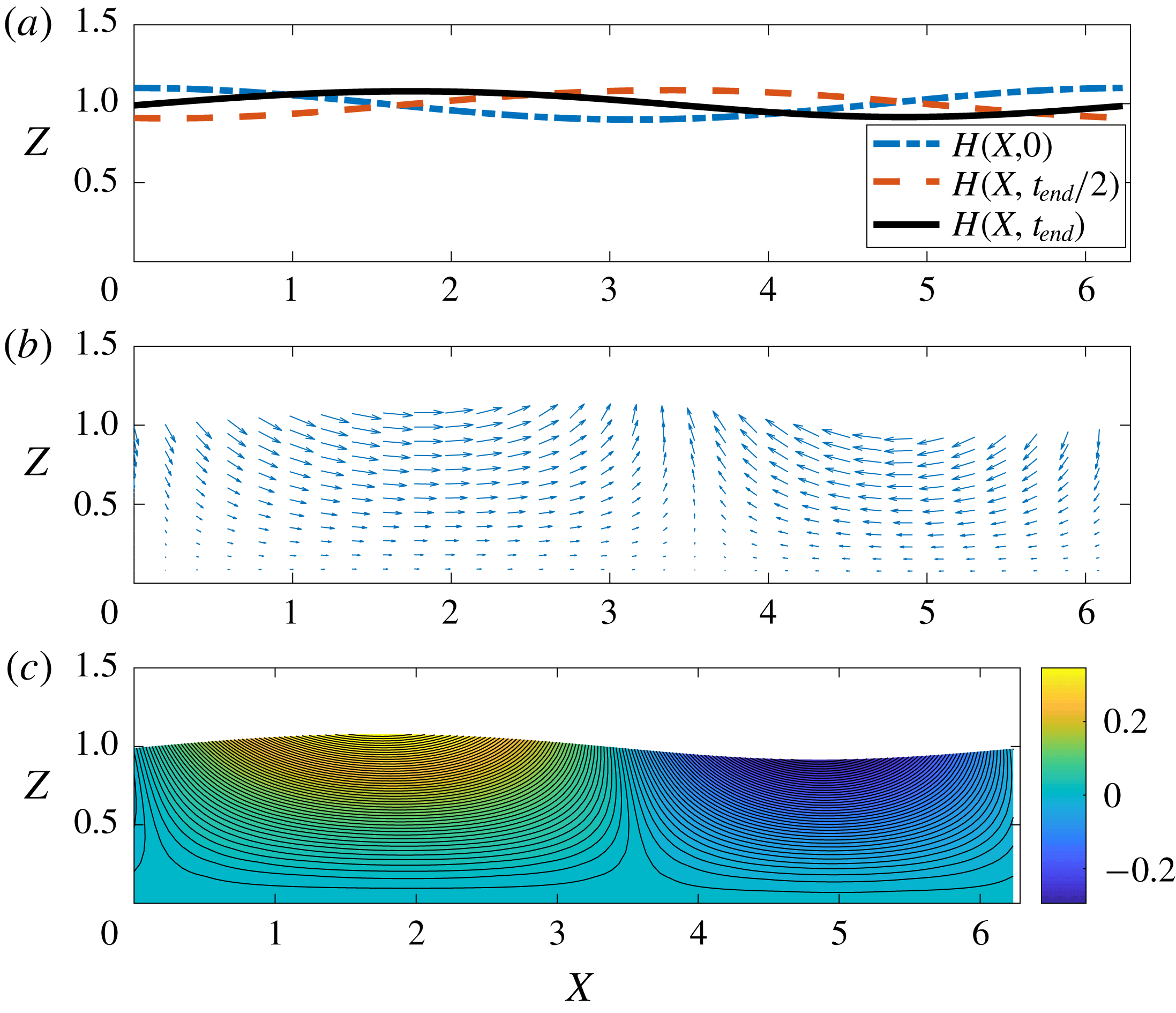
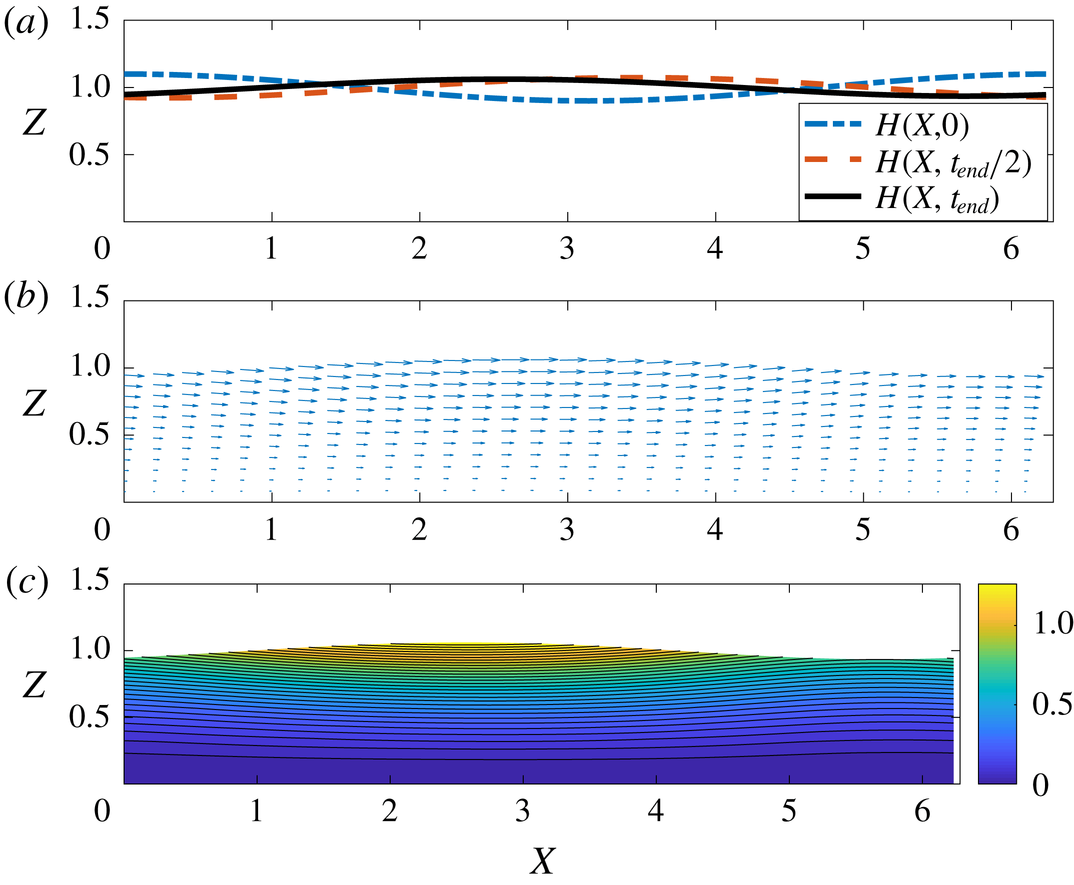
. This corresponds to a supercritical Hopf bifurcation. Figure 5 shows snapshots of the film propagating with velocity
$V$
. This behaviour corresponds to the film snapshots in figures 5(a) and 6(a).


Among these three cases one can find regimes where both parameters play a role in the stabilization of the liquid film. This behaviour corresponds to the film snapshots in figure 7(a).
To aid the reader, in appendix C we make a direct connection between the bifurcation criterion (5.12) and the Landau equation.
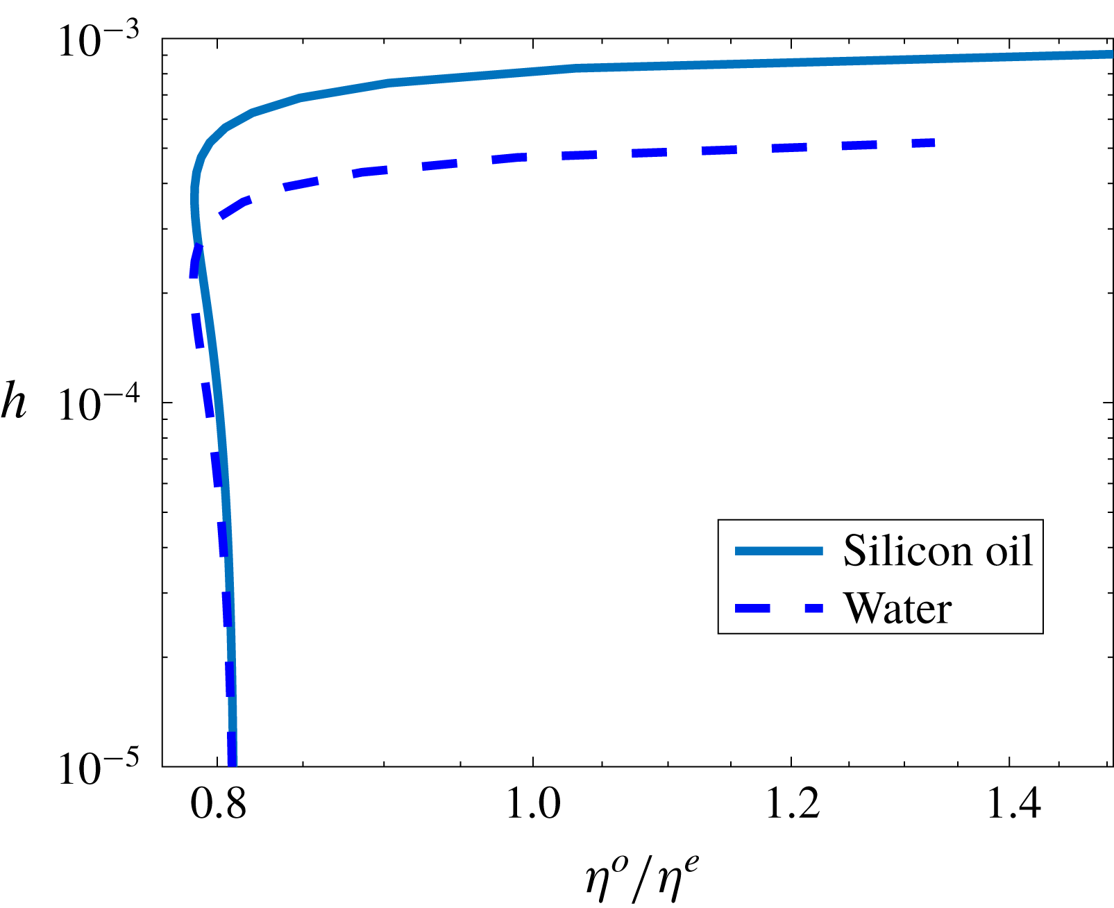
A wide range of values of the viscosity ratio versus the thickness of the film for two different liquids is displayed in figure 8 from (5.16). For the silicon oil with values taken from table 1 with film thickness
 $h=10^{-4}~\text{cm}$
and
 $\unicode[STIX]{x0394}\unicode[STIX]{x1D717}=20\,^{\circ }\text{C}$
we find
 $\unicode[STIX]{x1D706}=0.36~\text{cm}$
,
 $k_{cr}\text{(dimensional)}=24~\text{cm}^{-1}$
,
 $\unicode[STIX]{x1D716}=0.0017$
,
 $U_{0}=10~\text{cm}~\text{s}^{-1}$
and
 $\unicode[STIX]{x1D702}^{o}/\unicode[STIX]{x1D702}^{e}\sim 0.8$
.
A strong surface shear
 $\unicode[STIX]{x1D70F}=6$
(vanishing odd viscosity
 $\unicode[STIX]{x1D702}^{o}/\unicode[STIX]{x1D702}^{e}\equiv 0$
) suppresses the thermocapillary instability by inducing a permanent nonlinear viscous capillary wave on the liquid–gas interface. Numerical solutions of the evolution equation (3.15) with surface tension gradient
 $\unicode[STIX]{x1D6F4}_{X}$
from (3.14). (a) Snapshots of the wave profiles of the liquid–gas interface. (b) Velocity field at time
 $t_{end}$
. (c) Streamlines at time
 $t_{end}$
.

A non-zero odd viscosity,
 $\unicode[STIX]{x1D702}^{o}/\unicode[STIX]{x1D702}^{e}=3$
(vanishing surface shear
 $\unicode[STIX]{x1D70F}\equiv 0$
), suppresses the thermocapillary instability by inducing a permanent nonlinear dispersive capillary wave on the liquid–gas interface. Numerical solutions of the evolution equation (3.15) with surface tension gradient
 $\unicode[STIX]{x1D6F4}_{X}$
from (3.14). (a) Snapshots of the wave profiles of the liquid–gas interface. (b) Velocity field at time
 $t_{end}$
. (c) Streamlines at time
 $t_{end}$
.

A non-zero odd viscosity,
 $\unicode[STIX]{x1D702}^{o}/\unicode[STIX]{x1D702}^{e}=2$
, and non-zero surface shear
 $\unicode[STIX]{x1D70F}=2$
suppress the thermocapillary instability by inducing a permanent nonlinear dispersive capillary wave on the liquid–gas interface. Numerical solutions of the evolution equation (3.15) with surface tension gradient
 $\unicode[STIX]{x1D6F4}_{X}$
from (3.14). (a) Snapshots of the wave profiles of the liquid–gas interface. (b) Velocity field at time
 $t_{end}$
. (c) Streamlines at time
 $t_{end}$
.

Plot of the critical value of the viscosity ratio
 $\unicode[STIX]{x1D702}^{o}/\unicode[STIX]{x1D702}^{e}$
from (5.16) versus the dimensional film thickness
 $h$
for
 $\unicode[STIX]{x0394}\unicode[STIX]{x1D717}=20\,^{\circ }\text{C}$
and the two liquids whose natural properties appear in table 1.

Equation (2.37),
 $$\begin{eqnarray}H_{T}+\unicode[STIX]{x1D70F}HH_{X}+\left[\frac{1}{2}\unicode[STIX]{x1D6F4}_{X}H^{2}-\frac{1}{3}\left(\frac{\unicode[STIX]{x1D702}^{o}}{\unicode[STIX]{x1D702}^{e}}\unicode[STIX]{x1D6F4}_{XX}+GH_{X}-\bar{C}^{-1}H_{XXX}\right)H^{3}\right]_{X}=0,\end{eqnarray}$$
was solved numerically with periodic boundary conditions in a spatial domain of length corresponding to the wavenumber
 $k_{cr}$
from (4.2) and initial condition
 $H(X,0)=1+0.1\cos (k_{cr}X)$
. Here,
 $\unicode[STIX]{x1D6F4}_{X}$
is given by (3.14). We have performed standard pseudospectral Fourier computations in conjunction with one of MatLab’s variable time-stepping routines (Shampine & Reichelt Reference Shampine and Reichelt1997). We found that 128 nodes were sufficient to provide the sought spatial resolution. Following Kerchman & Frenkel (Reference Kerchman and Frenkel1994) we performed appropriate dealiasing. This is done by setting the Fourier coefficients of
 $H$
, and its derivatives corresponding to those high wavenumbers, equal to zero at each time-step and prior to calculating the nonlinear terms in physical space.
For values of the dimensionless variables
 $G=3,\bar{C}=1/3$
,
 $B=0.1$
and
 $M=4(B+1)^{2}/B$
the time variation of the liquid–gas interface
 $H(X,T)$
for
 $(\unicode[STIX]{x1D70F},\unicode[STIX]{x1D702}^{0})=(6,0)$
,
 $(\unicode[STIX]{x1D70F},\unicode[STIX]{x1D702}^{0})=(0,3\unicode[STIX]{x1D702}^{e})$
and
 $(\unicode[STIX]{x1D70F},\unicode[STIX]{x1D702}^{0})=(2,2\unicode[STIX]{x1D702}^{e})$
is displayed in figures 5(a), 6(a) and 7(a) respectively. In all cases stabilization has been reached.
6 Discussion
In this article we have examined the effect that odd viscosity has on the motion of a thin liquid film sitting on a solid substrate and surrounded by an ambient gas phase. New terms arise in the evolution equation of the liquid–gas interface that depend on odd viscosity. The free interface can support nonlinear viscous capillary waves that become prominent only when the surface shear stress at the liquid–gas interface is spatially dependent. We demonstrate this capacity of odd viscosity liquids by resorting to a thermocapillary system whose surface shear stress is spatially-dependent. Nonlinear wave propagation is possible because the surface tension gradient breaks the reflection symmetry of the evolution equation for the liquid–gas interface. Our main result is that for a certain regime of the ratio of viscosities the incipient surface wave propagation suppresses the thermocapillary instability.
The work discussed in this article can be expanded in a number of ways whenever surface shear stresses are spatially dependent. One such instance arises naturally in a liquid with rotational degrees of freedom, for example in a magnetic liquid, see Kirkinis (Reference Kirkinis2017). It also arises when one considers surface-active agents. In this case the surface tension gradient is proportional to the gradient of the adsorbed concentration, see for instance Oron et al. (Reference Oron, Davis and Bankoff1997).
Acknowledgements
The authors are grateful to three anonymous referees for their suggestions and criticism that significantly improved the manuscript. This work was supported by the US Department of Energy Office of Science, Basic Energy Sciences under Award no. DE-FG02-07ER46452.
Appendix A. Constitutive relations in the presence of a magnetic field
A magnetic field breaks the time-reversal symmetry and endows a liquid with an odd viscosity coefficient. In general the viscous stress tensor is of the form (Lifshitz & Pitaevskii Reference Lifshitz and Pitaevskii1981, § 13)
 $$\begin{eqnarray}\unicode[STIX]{x1D70E}_{\unicode[STIX]{x1D6FC}\unicode[STIX]{x1D6FD}}^{\prime }=\unicode[STIX]{x1D702}_{\unicode[STIX]{x1D6FC}\unicode[STIX]{x1D6FD}\unicode[STIX]{x1D6FE}\unicode[STIX]{x1D6FF}}V_{\unicode[STIX]{x1D6FE}\unicode[STIX]{x1D6FF}},\end{eqnarray}$$
where
 $V_{\unicode[STIX]{x1D6FE}\unicode[STIX]{x1D6FF}}={\textstyle \frac{1}{2}}((\unicode[STIX]{x2202}u_{\unicode[STIX]{x1D6FE}}/\unicode[STIX]{x2202}x_{\unicode[STIX]{x1D6FF}})+(\unicode[STIX]{x2202}u_{\unicode[STIX]{x1D6FF}}/\unicode[STIX]{x2202}x_{\unicode[STIX]{x1D6FE}}))$
. With the notation
 $\boldsymbol{b}=\boldsymbol{B}/B$
for the unit vector in the direction of the magnetic field
 $\boldsymbol{B}$
and for an incompressible liquid the viscous stress tensor is expressed in the form
 $$\begin{eqnarray}\displaystyle \unicode[STIX]{x1D70E}_{\unicode[STIX]{x1D6FC}\unicode[STIX]{x1D6FD}}^{\prime } & = & \displaystyle 2V_{\unicode[STIX]{x1D6FC}\unicode[STIX]{x1D6FD}}(\unicode[STIX]{x1D702}+\unicode[STIX]{x1D702}_{1})+V_{\unicode[STIX]{x1D6FD}\unicode[STIX]{x1D6FE}}[2(\unicode[STIX]{x1D702}_{2}-\unicode[STIX]{x1D702}_{1})b_{\unicode[STIX]{x1D6FE}}b_{\unicode[STIX]{x1D6FC}}+\unicode[STIX]{x1D702}_{3}b_{\unicode[STIX]{x1D6FC}\unicode[STIX]{x1D6FE}}]+V_{\unicode[STIX]{x1D6FC}\unicode[STIX]{x1D6FE}}[2(\unicode[STIX]{x1D702}_{2}-\unicode[STIX]{x1D702}_{1})b_{\unicode[STIX]{x1D6FE}}b_{\unicode[STIX]{x1D6FD}}+\unicode[STIX]{x1D702}_{3}b_{\unicode[STIX]{x1D6FD}\unicode[STIX]{x1D6FE}}]\nonumber\\ \displaystyle & & \displaystyle +\,V_{\unicode[STIX]{x1D6FE}\unicode[STIX]{x1D6FF}}[(\unicode[STIX]{x1D702}_{1}\!+\!\unicode[STIX]{x1D701}_{1})\unicode[STIX]{x1D6FF}_{\unicode[STIX]{x1D6FC}\unicode[STIX]{x1D6FD}}b_{\unicode[STIX]{x1D6FE}}b_{\unicode[STIX]{x1D6FF}}+(\unicode[STIX]{x1D702}_{1}-4\unicode[STIX]{x1D702}_{2})b_{\unicode[STIX]{x1D6FC}}b_{\unicode[STIX]{x1D6FD}}b_{\unicode[STIX]{x1D6FE}}b_{\unicode[STIX]{x1D6FF}}+(2\unicode[STIX]{x1D702}_{4}-\unicode[STIX]{x1D702}_{3})(b_{\unicode[STIX]{x1D6FC}\unicode[STIX]{x1D6FE}}b_{\unicode[STIX]{x1D6FD}}b_{\unicode[STIX]{x1D6FF}}\!+\!b_{\unicode[STIX]{x1D6FD}\unicode[STIX]{x1D6FE}}b_{\unicode[STIX]{x1D6FC}}b_{\unicode[STIX]{x1D6FF}})],\nonumber\\ \displaystyle & & \displaystyle\end{eqnarray}$$
where
 $b_{\unicode[STIX]{x1D6FC}\unicode[STIX]{x1D6FD}}=\unicode[STIX]{x1D716}_{\unicode[STIX]{x1D6FC}\unicode[STIX]{x1D6FD}\unicode[STIX]{x1D6FE}}b_{\unicode[STIX]{x1D6FE}}$
and
 $\unicode[STIX]{x1D702}_{i},\unicode[STIX]{x1D701}_{i}$
are viscosity coefficients. For the geometry considered in this article and for a magnetic field in the
 $y$
-direction, setting
 $b_{2}=b$
and considering the long-wavelength approximation we obtain
 $$\begin{eqnarray}\unicode[STIX]{x1D70E}_{13}=\unicode[STIX]{x1D70E}_{31}=(\unicode[STIX]{x1D702}+\unicode[STIX]{x1D702}_{1})u_{z},\quad \unicode[STIX]{x1D70E}_{33}=-\unicode[STIX]{x1D70E}_{11}=\unicode[STIX]{x1D702}_{3}bu_{z}.\end{eqnarray}$$
Comparing these expressions with (2.4) leads to the identification
 $\unicode[STIX]{x1D702}^{o}\equiv \unicode[STIX]{x1D702}_{3}b$
.
The heat flux
 $\boldsymbol{q}$
, in the presence of a magnetic field, becomes (Lifshitz & Pitaevskii Reference Lifshitz and Pitaevskii1981, § 13)
 $$\begin{eqnarray}\boldsymbol{q}=-k_{th}\unicode[STIX]{x1D735}\unicode[STIX]{x1D717}-\unicode[STIX]{x1D705}_{1}\boldsymbol{b}(\boldsymbol{b}\boldsymbol{\cdot }\unicode[STIX]{x1D735}\unicode[STIX]{x1D717})-\unicode[STIX]{x1D705}_{2}\unicode[STIX]{x1D735}\unicode[STIX]{x1D717}\times \boldsymbol{b},\end{eqnarray}$$
for the thermal conductivities
 $k_{th}$
and
 $\unicode[STIX]{x1D705}_{i}$
. With respect to the conditions mentioned above, the two components of
 $\boldsymbol{q}$
become
 $$\begin{eqnarray}q_{1}=-k_{th}\unicode[STIX]{x1D717}_{x}+\unicode[STIX]{x1D705}_{2}b\unicode[STIX]{x1D717}_{z}\quad \text{and}\quad q_{3}=-\unicode[STIX]{x1D705}_{2}b\unicode[STIX]{x1D717}_{x}-k_{th}\unicode[STIX]{x1D717}_{z},\end{eqnarray}$$
so that
 $$\begin{eqnarray}-\text{div}\boldsymbol{q}=k_{th}\unicode[STIX]{x1D717}_{xx}-\unicode[STIX]{x1D705}_{2}b\unicode[STIX]{x1D717}_{xz}+\unicode[STIX]{x1D705}_{2}b\unicode[STIX]{x1D717}_{zx}+k_{th}\unicode[STIX]{x1D717}_{zz}.\end{eqnarray}$$
Thus, in the long-wavelength limit, only the last term on the right-hand side of (A 6) is of order one and this recovers the energy equation (3.7). Similarly, the boundary condition
 $\boldsymbol{n}\boldsymbol{\cdot }\unicode[STIX]{x1D735}\boldsymbol{q}=\unicode[STIX]{x1D6FC}_{th}(\unicode[STIX]{x1D717}-\unicode[STIX]{x1D717}_{\infty })$
at the liquid–gas interface reduces to (3.8).
Appendix B. Non-dissipative nature of odd viscosity: absence of viscous heating
An alternative argument to the existing ones regarding the non-dissipative nature of odd viscosity is that it does not raise the temperature of a liquid. From Landau & Lifshitz (Reference Landau and Lifshitz1987) equation (50.1) we know that the energy equation of a moving liquid with heat conduction and viscous heating is
 $$\begin{eqnarray}\unicode[STIX]{x1D70C}c_{p}(\unicode[STIX]{x1D717}_{t}+\boldsymbol{u}\boldsymbol{\cdot }\text{grad}\unicode[STIX]{x1D717})=k\unicode[STIX]{x1D6FB}^{2}\unicode[STIX]{x1D717}+\unicode[STIX]{x1D70E}_{ik}^{\prime }\frac{\unicode[STIX]{x2202}u_{i}}{\unicode[STIX]{x2202}x_{k}},\end{eqnarray}$$
where
 $$\begin{eqnarray}\unicode[STIX]{x1D70E}_{ik}^{\prime }=\unicode[STIX]{x1D702}^{e}\left(\frac{\unicode[STIX]{x2202}u_{i}}{\unicode[STIX]{x2202}x_{k}}+\frac{\unicode[STIX]{x2202}u_{k}}{\unicode[STIX]{x2202}x_{i}}\right)+\unicode[STIX]{x1D70E}_{ik}^{o},\end{eqnarray}$$
(see (2.2) and (2.3)). Employing expression (2.3) for the odd part of the stress tensor and after some rearrangement and symmetrization (B 1) becomes
 $$\begin{eqnarray}\unicode[STIX]{x1D70C}c_{p}(\unicode[STIX]{x1D717}_{t}+\boldsymbol{u}\boldsymbol{\cdot }\text{grad}\unicode[STIX]{x1D717})=k\unicode[STIX]{x1D6FB}^{2}\unicode[STIX]{x1D717}+\frac{\unicode[STIX]{x1D702}^{e}}{2}\left(\frac{\unicode[STIX]{x2202}u_{i}}{\unicode[STIX]{x2202}x_{k}}+\frac{\unicode[STIX]{x2202}u_{k}}{\unicode[STIX]{x2202}x_{i}}\right)^{2},\end{eqnarray}$$
which shows that only the part of the stress tensor associated with the even viscosity can raise the temperature of a liquid. One would expect this result also on the basis of vanishing surface terms (that contain the pressure multiplied by velocity) in the energy equation. See equation (16.2) of Landau & Lifshitz (Reference Landau and Lifshitz1987).
Following the same line of arguments one can show that the evolution of the entropy in a liquid with heat conduction is also not affected by odd viscosity, whether the liquid is incompressible or not, see equations (49.4) and (49.5) in Landau & Lifshitz (Reference Landau and Lifshitz1987).
Still the same arguments lead to the conclusion that energy dissipation leads to a decrease in mechanical energy (cf. equation (16.3) in Landau & Lifshitz (Reference Landau and Lifshitz1987))
 $$\begin{eqnarray}{\dot{E}}_{\text{kin}}=-\frac{1}{2}\unicode[STIX]{x1D702}^{e}\int \left(\frac{\unicode[STIX]{x2202}u_{i}}{\unicode[STIX]{x2202}x_{k}}+\frac{\unicode[STIX]{x2202}u_{k}}{\unicode[STIX]{x2202}x_{i}}\right)^{2}\text{d}^{3}x,\end{eqnarray}$$
so that the even coefficient of viscosity is always positive.
Appendix C. Derivation of the Landau equation
To understand the logic behind the bifurcation criterion (5.12) we return to our discussion of § 5.2 and derive the Landau equation. Expand
 $H$
about a steady state
 $$\begin{eqnarray}\displaystyle H & = & \displaystyle 1+\unicode[STIX]{x1D6FF}[A_{1}(\unicode[STIX]{x1D6FF}^{2}T)\text{e}^{\text{i}q(X-VT)}+A_{1}^{\ast }(\unicode[STIX]{x1D6FF}^{2}T)\text{e}^{-\text{i}q(X-VT)}]\nonumber\\ \displaystyle & & \displaystyle +\,\unicode[STIX]{x1D6FF}^{2}[A_{2}(\unicode[STIX]{x1D6FF}^{2}T)\text{e}^{2\text{i}q(X-VT)}+A_{2}^{\ast }(\unicode[STIX]{x1D6FF}^{2}T)\text{e}^{-2\text{i}q(X-VT)}]+O(\unicode[STIX]{x1D6FF}^{3}),\end{eqnarray}$$
for complex amplitudes
 $A_{1},A_{2}$
etc. where
 $V$
is given by (5.11a
). Introduce the bifurcation parameter
 $$\begin{eqnarray}\unicode[STIX]{x1D707}=\frac{M-M_{cr}}{M_{cr}}\end{eqnarray}$$
and expand in
 $\unicode[STIX]{x1D6FF}$
so that
 $\unicode[STIX]{x1D707}=\unicode[STIX]{x1D707}_{0}+\unicode[STIX]{x1D6FF}^{2}\unicode[STIX]{x1D707}_{2}+\cdots \,$
. This means that the expansion parameter
 $\unicode[STIX]{x1D6FF}$
is defined by
 $$\begin{eqnarray}\unicode[STIX]{x1D6FF}^{2}=\frac{\unicode[STIX]{x1D707}-\unicode[STIX]{x1D707}_{0}}{\unicode[STIX]{x1D707}_{2}}.\end{eqnarray}$$
The slow time dependence
 $\unicode[STIX]{x1D6FF}^{2}T$
is suggested by the linearized theory indicating that the amplitude of the critical mode is a function of
 $|M-M_{cr}|T$
as
 $|M-M_{cr}|\rightarrow 0$
(Erneux & Davis Reference Erneux and Davis1993).
In (3.15) we set
 $\unicode[STIX]{x1D70F}\equiv 0$
to simplify the presentation. Substituting (C 1) into (3.15) leads to a Landau equation for the amplitude
 $A_{1}$
. Setting
 $A_{1}=R\text{e}^{\text{i}\unicode[STIX]{x1D711}}$
and solving for the real part of the Landau equation we obtain
 $$\begin{eqnarray}\displaystyle \frac{\text{d}R}{\text{d}\hat{T}} & = & \displaystyle \frac{\unicode[STIX]{x1D707}_{2}q^{2}G}{3}R+\frac{q^{2}}{18\bar{C}\left(9\,q^{2}+(\bar{C}G+q^{2})^{2}\left({\displaystyle \frac{\unicode[STIX]{x1D702}^{o}}{\unicode[STIX]{x1D702}^{e}}}\right)^{2}\right)(B+1)^{2}}\nonumber\\ \displaystyle & & \displaystyle \times \left(\!2(\bar{C}G+q^{2})^{2}(27B^{2}\bar{C}G+35B^{2}q^{2}+42B\bar{C}G+30Bq^{2}+12\bar{C}G-24q^{2})\!\!\left({\displaystyle \frac{\unicode[STIX]{x1D702}^{o}}{\unicode[STIX]{x1D702}^{e}}}\right)^{\!2}\right.\nonumber\\ \displaystyle & & \displaystyle +\left.9(\bar{C}G+q^{2})(9B^{2}\bar{C}G+45B^{2}q^{2}+6B\bar{C}G+30Bq^{2}+\bar{C}G+7q^{2})\vphantom{\left({\displaystyle \frac{\unicode[STIX]{x1D702}^{o}}{\unicode[STIX]{x1D702}^{e}}}\right)^{2}}\right)R^{3}.\end{eqnarray}$$
Equation (C 4) is of the general form
 $$\begin{eqnarray}\frac{\text{d}R}{\text{d}\hat{T}}=\unicode[STIX]{x1D6FC}R-\unicode[STIX]{x1D6FD}R^{3},\end{eqnarray}$$
where the coefficients
 $\unicode[STIX]{x1D6FC}$
and
 $\unicode[STIX]{x1D6FD}$
can be read off from (C 4) and
 $\hat{T}=\unicode[STIX]{x1D6FF}^{2}T$
. When the parameters
 $\unicode[STIX]{x1D6FC}$
and
 $\unicode[STIX]{x1D6FD}$
are positive (equivalently when the bifurcation parameter
 $a_{2}$
in (5.12) is positive), the Landau equation acquires the (stable) steady-state solution
 $$\begin{eqnarray}R=\sqrt{\frac{\unicode[STIX]{x1D6FC}}{\unicode[STIX]{x1D6FD}}},\end{eqnarray}$$
observed in the numerical simulations. When
 $a_{2}<0$
no such steady-state solutions exist. The equivalence between the right-hand side of (C 4) and (5.12) can be established by setting
 $R=\sqrt{A_{c}^{2}+A_{s}^{2}}/2$
.