2 Direct numerical simulations of polymeric solutions

The mean momentum equation based analysis is conducted using datasets from DNS simulations of viscoelastic turbulent channel flow from two independent research groups. The parameters and the data symbols associated with the datasets are summarized in table 1. The datasets were selected because they span almost a decade in $\unicode[STIX]{x1D6FF}^{+}$ . For ease of interpretation, and when appropriate, the datasets may be segregated by DR into three categories: Newtonian flow ( $\text{DR}=0\,\%$ ), low drag reduction, LDR, ( $0<\text{DR}\leqslant 40\,\%$ ), high drag reduction, HDR, ( $\text{DR}>40\,\%$ ). Alternatively, the datasets from Dubief et al. (Reference Dubief, White, Terrapon, Shaqfeh, Moin and Lele2004), Thais et al. (Reference Thais, Tejada-Mart́inez, Gatski and Mompean2011) and Dubief, Terrapon & Soria (Reference Dubief, Terrapon and Soria2013), Thais, Gatski & Mompean (Reference Thais, Gatski and Mompean2013) may be presented separately. In addition, only representative datasets from the 13 total datasets may be presented.

Table 1.

Data symbols and parameters for the viscoelastic simulations. The Weissenberg number $We_{\unicode[STIX]{x1D70F}}=\unicode[STIX]{x1D706}u_{\unicode[STIX]{x1D70F}}^{2}/\unicode[STIX]{x1D708}_{o}$ , where $\unicode[STIX]{x1D708}_{0}$ is the zero shear rate kinematic viscosity of the solution.

The numerical methods used by the two research groups, described in Dubief et al. (Reference Dubief, White, Terrapon, Shaqfeh, Moin and Lele2004, Reference Dubief, Terrapon, White, Shaqfeh, Moin and Lele2005, Reference Dubief, Terrapon and Soria2013) and Thais et al. (Reference Thais, Tejada-Mart́inez, Gatski and Mompean2011, Reference Thais, Gatski and Mompean2013), are briefly reviewed here. The channel flow simulations employ a Cartesian domain defined by the orthonormal vector base $(\boldsymbol{e}_{x},\boldsymbol{e}_{y},\boldsymbol{e}_{z})$ where $x$ , $y$ and $z$ are the streamwise, wall-normal and spanwise directions, respectively. The components of the velocity vector $\boldsymbol{u}$ are $u$ , $v$ and $w$ . For a viscoelastic flow, the governing equations for conservation of mass and transport of momentum are

(2.1) $$\begin{eqnarray}\displaystyle & \displaystyle \unicode[STIX]{x1D735}\boldsymbol{\cdot }\boldsymbol{u}=0\quad \text{and} & \displaystyle\end{eqnarray}$$

(2.2) $$\begin{eqnarray}\displaystyle & \displaystyle \frac{\unicode[STIX]{x2202}\boldsymbol{u}}{\unicode[STIX]{x2202}t}+(\boldsymbol{u}\boldsymbol{\cdot }\unicode[STIX]{x1D735})\boldsymbol{u}=-\unicode[STIX]{x1D735}p+\frac{\unicode[STIX]{x1D6FE}}{Re}\unicode[STIX]{x1D6FB}^{2}\boldsymbol{u}+\frac{1-\unicode[STIX]{x1D6FE}}{Re}\unicode[STIX]{x1D735}\boldsymbol{\cdot }\unicode[STIX]{x1D733}+g(t)\boldsymbol{e}_{x}, & \displaystyle\end{eqnarray}$$

where $t$ is time, $p$ is the hydrostatic pressure, $\unicode[STIX]{x1D6FE}$ is the ratio of solvent viscosity to the zero-shear viscosity of the polymer solution, $\unicode[STIX]{x1D733}$ is the polymer stress tensor and $g(t)$ is the pressure gradient driving the flow. The polymer stress tensor $\unicode[STIX]{x1D733}$ is computed using the FENE-P (Finite Elastic Nonlinear Extensibility-Peterlin) model

(2.3) $$\begin{eqnarray}\unicode[STIX]{x1D733}=\frac{1}{We}\left(\frac{\unicode[STIX]{x1D63E}}{1-\text{tr}(\unicode[STIX]{x1D63E})/L^{2}}-\unicode[STIX]{x1D644}\right),\end{eqnarray}$$

where the tensor $\unicode[STIX]{x1D63E}$ is the local conformation tensor of the polymer solution and $\unicode[STIX]{x1D644}$ is the unit tensor. The properties of the polymer solution are $\unicode[STIX]{x1D6FE}$ , the maximum polymer extension $L$ , and the relaxation time $\unicode[STIX]{x1D706}$ , based on the convection scales Weissenberg number ( $We=\unicode[STIX]{x1D706}U_{c}/\unicode[STIX]{x1D6FF}$ ) where $U_{c}$ is the centreline velocity, $\unicode[STIX]{x1D6FF}$ the channel half-height. The FENE-P models a polymer molecule by a pair of beads connected by a nonlinear spring defined by the end-to-end vector $\boldsymbol{q}$ . The conformation tensor is the phase average of the tensorial product of the end-to-end vector $\boldsymbol{q}$ with itself, $\unicode[STIX]{x1D63E}=\langle \boldsymbol{q}\otimes \boldsymbol{q}\rangle$ whose transport equation is

(2.4) $$\begin{eqnarray}\frac{\unicode[STIX]{x2202}\unicode[STIX]{x1D63E}}{\unicode[STIX]{x2202}t}+(\boldsymbol{u}\boldsymbol{\cdot }\unicode[STIX]{x1D735})\unicode[STIX]{x1D63E}=\unicode[STIX]{x1D63E}(\unicode[STIX]{x1D735}\,\boldsymbol{u})+(\unicode[STIX]{x1D735}\,\boldsymbol{u})^{\text{T}}\unicode[STIX]{x1D63E}-\unicode[STIX]{x1D733}.\end{eqnarray}$$

Equations (2.2)–(2.4) with appropriate boundary conditions are solved using slightly different numerical methods between the two research groups. The datasets of Thais et al. (Reference Thais, Tejada-Mart́inez, Gatski and Mompean2011) were obtained using a hybrid spatial scheme with Fourier spectral discretization in the two homogeneous directions and high-order finite differences in the wall-normal direction. This approach was chosen to efficiently simulate high $\unicode[STIX]{x1D6FF}^{+}$ flows. The datasets of Dubief et al. (Reference Dubief, White, Terrapon, Shaqfeh, Moin and Lele2004, Reference Dubief, Terrapon and Soria2013) were obtained using finite differences on a staggered grid and a compact upwind scheme for the polymer advection term. The latter avoids the need to add a global artificial dissipation term to the transport equation for the confirmation tensor (2.4). The inclusion of a dissipation term to (2.4) is a common approach used to achieve code stability when simulating high $We$ flows using pseudo-spectral methods (Sureshkumar & Boris Reference Sureshkumar and Boris1995). See Dubief et al. (Reference Dubief, Terrapon, White, Shaqfeh, Moin and Lele2005) and Thais et al. (Reference Thais, Tejada-Mart́inez, Gatski and Mompean2011) for detailed descriptions of the numerical methods and their validation.

Figure 1.

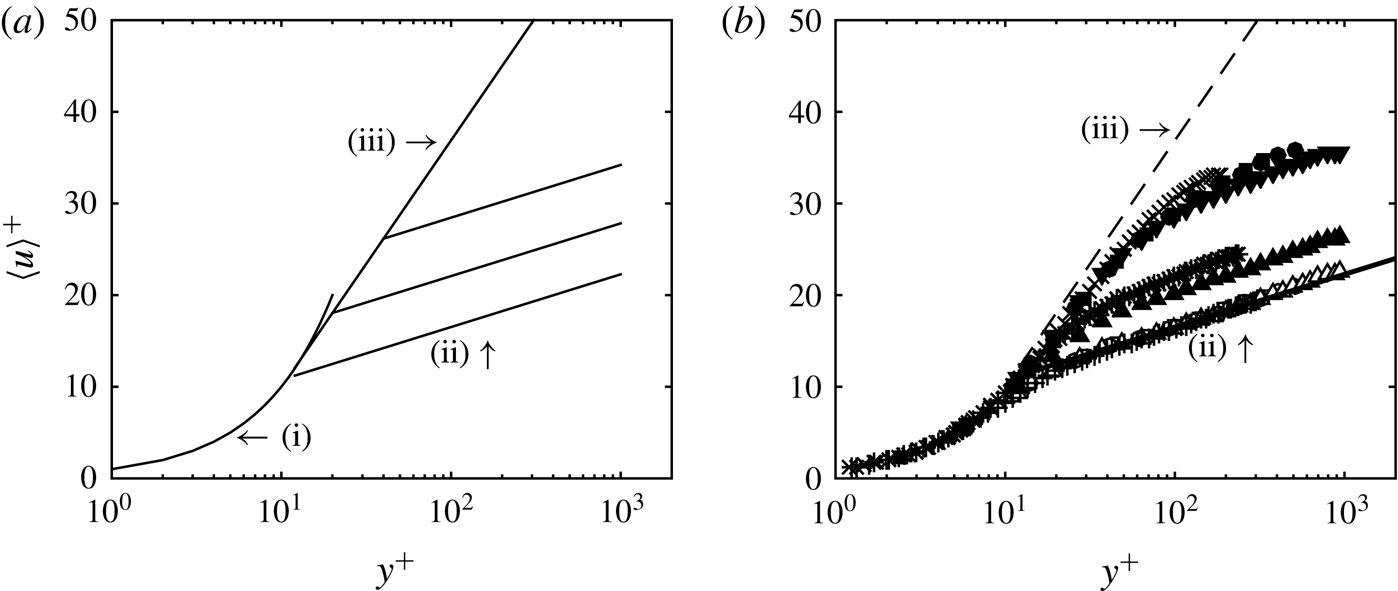
(a) Schematic of the behaviours of the mean velocity distribution for wall-bounded flow of polymer solutions as summarized by Virk (Reference Virk1975): (i) $\langle u\rangle ^{+}=y^{+}$ , (ii) is the Newtonian ‘law of the wall’ given by $\langle u\rangle ^{+}=2.5\log (y^{+})+5.0$ , and (iii) is the ‘ultimate profile’ given by (3.2). With DR, the mean velocity distribution initially follows (iii) and then crosses over to a ‘Newtonian plug flow’ with the same value of $\unicode[STIX]{x1D705}$ as (ii) and $C_{1}$ increasing with increasing DR. (b) Mean velocity profiles of DNS datasets tabulated in table 1.

3 Behaviours of the mean velocity distribution in polymeric flows

The earliest description of the collective behaviours of the mean velocity distribution in polymer drag-reduced flow was given by Virk (Reference Virk1975), and explained here with reference to figure 1(a). The figure illustrates distributions of mean velocity in wall coordinates for turbulent pipe flow of polymer solution at varying DR, where the superscript $^{+}$ denotes normalization by the friction velocity $u_{\unicode[STIX]{x1D70F}}=\sqrt{\unicode[STIX]{x1D70F}_{w}/\unicode[STIX]{x1D70C}}$ and kinematic viscosity $\unicode[STIX]{x1D708}$ , where $\unicode[STIX]{x1D70F}_{w}$ is the shear stress at the wall and $\unicode[STIX]{x1D70C}$ the fluid density. In semi-log coordinates, regions of constant slope are suggestive of logarithmic dependence of the mean velocity. i.e.

(3.1) $$\begin{eqnarray}\langle u\rangle ^{+}=\frac{1}{\unicode[STIX]{x1D705}}\ln (y^{+})+C_{1},\end{eqnarray}$$

where $\langle \cdot \rangle$ denotes an average, $1/\unicode[STIX]{x1D705}$ (typically $\unicode[STIX]{x1D705}$ is called the von Kármán coefficient) is the slope and $C_{1}$ is the intercept at $y^{+}=1$ . For Newtonian fluids over hydraulically smooth walls, equation (3.1) is often referred to as the logarithmic ‘law of the wall’ with constants (at sufficiently high Reynolds number) $\unicode[STIX]{x1D705}\approx 0.4$ and $C_{1}\approx 5$ , with some existing evidence for variations depending on the canonical flow type (Nagib & Chauhan Reference Nagib and Chauhan2008). The polymer drag-reduced pipe flow data compiled by Virk (Reference Virk1975) suggest logarithmic behaviours of the mean velocity distribution that vary with the DR achieved. At maximum drag reduction (MDR), the entire profile outside of the viscous sublayer appears logarithmic and adheres to the ‘ultimate profile’ determined empirically by Virk et al. (Reference Virk, Mickley and Smith1970) as

(3.2) $$\begin{eqnarray}\langle u\rangle ^{+}=11.7\ln (y^{+})-17.\end{eqnarray}$$

It follows that a friction factor relation at MDR can be obtained by assuming equation (3.2) holds across the entire pipe. This friction relation is the so-called MDR asymptote and is given by

(3.3) $$\begin{eqnarray}\frac{1}{\sqrt{f}}=19\log Re\sqrt{f}-32.4,\end{eqnarray}$$

where the friction factor $f=2u_{\unicode[STIX]{x1D70F}}^{2}/U_{b}^{2}$ , $U_{b}$ is the bulk velocity in the pipe, and the Reynolds number $Re=U_{b}D/\unicode[STIX]{x1D708}$ where $D$ is the pipe diameter. Equations (3.2) and (3.3) are commonly believed to be approximately universal and insensitive to polymer species, molecular weight or the polymer–solvent pair. For intermediate DR, the mean velocity profile is described as initially following (3.2) and then is described as crossing over to a ‘Newtonian plug flow’ with the same value of $\unicode[STIX]{x1D705}$ as that for wall-bounded flows of Newtonian fluids and $C_{1}$ increasing with increasing DR. At zero DR, the mean velocity profile of a polymer solution follows that of a Newtonian fluid.

The inner-normalized mean velocity profiles from the DNS datasets tabulated in table 1 are shown in figure 1(b). In general, the behaviours of the mean velocity profiles with increasing DR appear to be generally well captured by the schematic in figure 1(a). Consequently, it is clear why Virk’s description of the collective behaviours of the mean velocity distribution in polymer drag-reduced flow has endured for more than 40 years. Nevertheless, as pointed out by White et al. (Reference White, Dubief and Klewicki2012), there have been several studies over these 40 years that have reported discrepancies between measured velocity profiles and Virk’s model. This includes profiles with slopes not quite parallel to the Newtonian log law, and profiles with slopes greater than 11.7 at maximum drag reduction. Often, these discrepancies were attributed to measurement uncertainty or second-order effects not captured by Virk’s model. In addition, close inspection of the DNS profiles in figure 1(b) show that for the HDR flows, the slope increases relative to the Newtonian case, but is less than the slope given by (3.2). Similar observations have led to the common belief that there is a difference between LDR and HDR flows (Warholic, Massah & Hanratty Reference Warholic, Massah and Hanratty1999; Dubief et al. Reference Dubief, White, Terrapon, Shaqfeh, Moin and Lele2004).

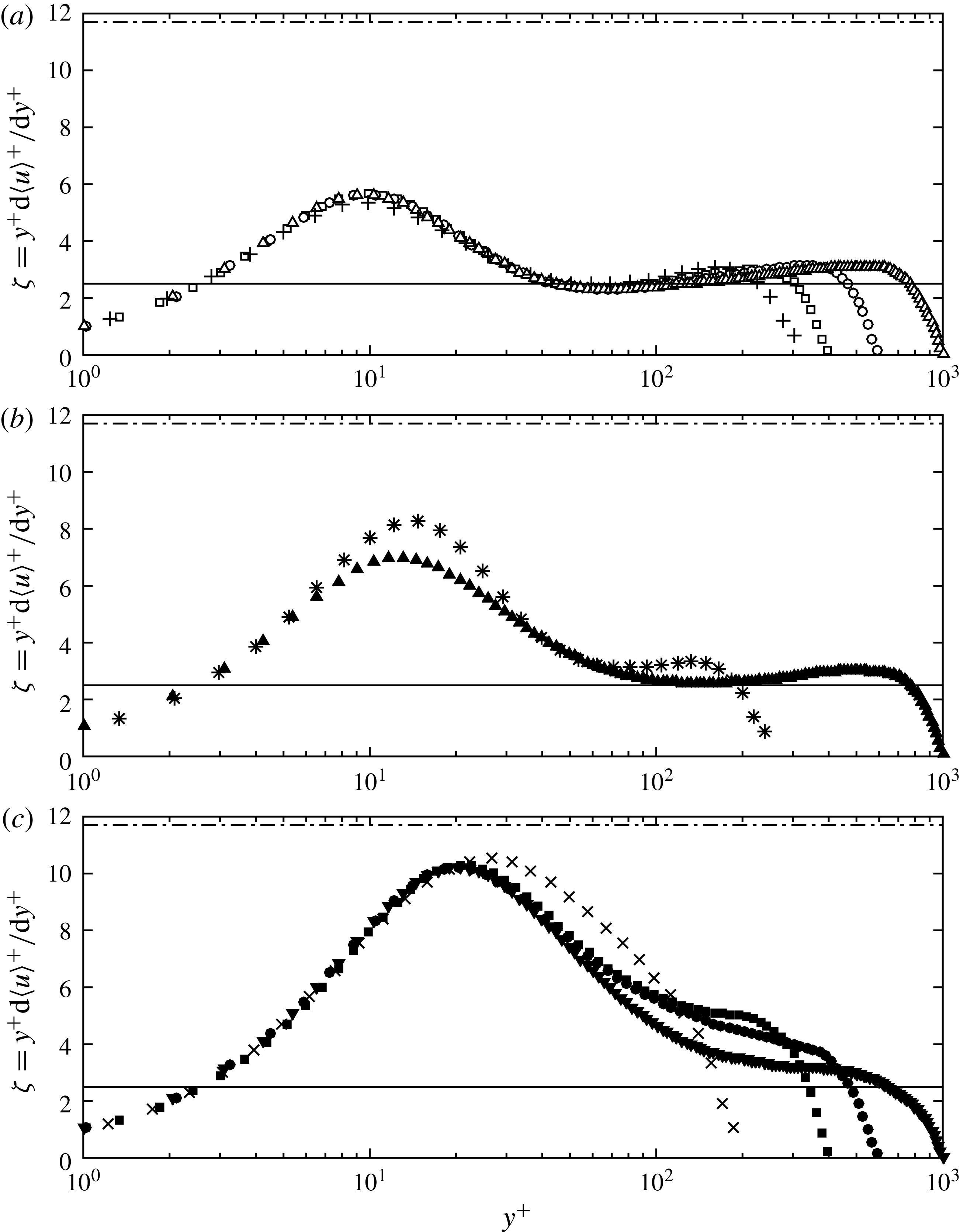
Following White et al. (Reference White, Dubief and Klewicki2012), the influence of polymer on the mean velocity distribution is evaluated using the so-called indicator function, $\unicode[STIX]{x1D701}=y^{+}\,\text{d}\langle u\rangle ^{+}/\text{d}y^{+}$ , typically used to investigate logarithmic dependence of the mean velocity profile. Profiles of $\unicode[STIX]{x1D701}$ for the DNS datasets are shown in figure 2. To frame the discussion, note that a region of local minima approaching constancy indicates logarithmic dependence of the mean velocity in an interior inertial region of the flow (i.e. the so-called inertial sublayer), where the approximately constant value corresponds to $1/\unicode[STIX]{x1D705}$ . The near-wall maximum in $\unicode[STIX]{x1D701}$ is nominally centred in the so-called buffer layer. Note that the mean velocity distribution in the buffer layer appears logarithmic in wall coordinates, but is clearly not logarithmic as illustrated by the parabolic shape of $\unicode[STIX]{x1D701}$ in the buffer region.

The Newtonian $\unicode[STIX]{x1D701}$ profiles show a clear $\unicode[STIX]{x1D6FF}^{+}$ dependence. Here the log layer moves outward from the wall and $\unicode[STIX]{x1D705}$ decreases with increasing $\unicode[STIX]{x1D6FF}^{+}$ , consistent with the results of Nagib & Chauhan (Reference Nagib and Chauhan2008). For the LDR $\unicode[STIX]{x1D701}$ profiles, the log layer is farther from the wall and the slope is modified (larger) compared to the Newtonian case at a similar $\unicode[STIX]{x1D6FF}^{+}$ . Importantly, the HDR $\unicode[STIX]{x1D701}$ profiles do not show a region of local minima in the interior region of the flow, indicating that the mean velocity distribution does not possess an inertially dominated logarithmic region (i.e. it has been eradicated by the action of the polymers). Consequently, the mean velocity profile in polymer HDR flow is not accurately captured by a logarithmic function. Instead, the $\unicode[STIX]{x1D701}$ profiles show that the apparent logarithmic-like behaviours of the HDR mean velocity profiles correspond to a thickened buffer layer. (Virk (Reference Virk1975) termed the extended buffer layer the elastic sublayer.) It follows that the slope of the ultimate profile (i.e. 11.7 and shown as a horizontal dashed-dotted line in figure 2) corresponds to an approximate peak value of $\unicode[STIX]{x1D701}$ in the extended buffer layer at maximum drag reduction. These data also suggest that this peak value is likely not universal, but depends on $\unicode[STIX]{x1D6FF}^{+}$ and possibly polymeric properties (White et al. Reference White, Dubief and Klewicki2012). Since the mean velocity profile at MDR is not precisely described by (3.2), it follows that the friction relation at MDR is not precisely described by (3.3).

Figure 2.

Indicator function typically used to investigate logarithmic dependence of the mean velocity profile. (a) Newtonian channel flow, (b) LDR viscoelastic channel flow, (c) HDR viscoelastic channel flow. Symbol key is given in table 1. The — corresponds to 2.5 and — ⋅ — corresponds to 11.7.

The $\unicode[STIX]{x1D701}$ profiles shown in figure 2 provide clear evidence that, with increasing DR, the action of polymers first modify then eliminate the inertially dominated logarithmic region of the flow. It then follows that the state of maximum drag reduction is attained only after the inertial sublayer is eradicated. Since the existence and behaviours of the inertial layer are a manifestation of the underlying dynamical behaviours of turbulent wall-bounded flow, understanding how polymers modify the inertial layer should be inherently important to understanding the dynamics of polymer drag reduced flow, and, consequently, the phenomenon of polymer drag reduction. The goal of the present study is to employ the mean momentum equation based framework to gain an improved understanding of the effects of polymers on the mean dynamics of the inertial layer.

4 The mean momentum equation based framework

A description of the mean momentum equation analysis framework can be found in Fife et al. (Reference Fife, Wei, Klewicki and Mcmurtry2005), Wei et al. (Reference Wei, Fife, Klewicki and Mcmurtry2005), Fife, Klewicki & Wei (Reference Fife, Klewicki and Wei2009), Klewicki et al. (Reference Klewicki, Fife and Wei2009), Klewicki, Ebner & Wu (Reference Klewicki, Ebner and Wu2011), Klewicki (Reference Klewicki2013), among others. Nevertheless, to keep the article self-contained and to provide a useful context relative to the mean dynamics in polymer drag-reduced flow, we first provide a condensed description of the framework applied to the Newtonian DNS channel flow simulations listed in table 1.

4.1 Mean dynamics of Newtonian channel flow

For a canonical turbulent channel flow of channel half-height $\unicode[STIX]{x1D6FF}$ the inner-normalized mean momentum equation is given by

(4.1) $$\begin{eqnarray}0=\underbrace{\frac{1}{\unicode[STIX]{x1D6FF}^{+}}}_{A}+\underbrace{\frac{\text{d}^{2}\langle u\rangle ^{+}}{\text{d}y^{+2}}}_{B}-\underbrace{\frac{\text{d}\langle u^{\prime }v^{\prime }\rangle ^{+}}{\text{d}y^{+}}}_{C}.\end{eqnarray}$$

Three physical mechanisms are represented from left to right in (4.1): term $A$ is the mean pressure gradient, term $B$ is the mean viscous force, term $C$ is the net mean effect of turbulent inertia. The mean effect of turbulent inertia (term $C$ ) becomes non-zero shortly after the onset of the transition to turbulence. This quantity increases in magnitude with increasing Reynolds number, and owing to the constancy of the mean pressure gradient (at any given $\unicode[STIX]{x1D6FF}^{+}$ ), the mean viscous force responds in accord with the balance expressed by (4.1). At $\unicode[STIX]{x1D6FF}^{+}\simeq 180$ , the terms in (4.1) begin to nominally satisfy the four layer magnitude ordering of terms first revealed by Wei et al. (Reference Wei, Fife, Klewicki and Mcmurtry2005) that is characteristic of the flow for all higher $\unicode[STIX]{x1D6FF}^{+}$ (Klewicki et al. Reference Klewicki, Ebner and Wu2011). The four layer structure is revealed through the ratio $B/C$ as shown in figure 3. Within three sub-regions (4.1) is brought into balance owing to two large terms and one small term (layers I, II and IV, see figure 3 b), while in another sub-region (layer III) all three terms continue to contribute significantly to the balance. Thus, while all of the terms in (4.1) are of leading order over some portion of $0\leqslant y\leqslant \unicode[STIX]{x1D6FF}$ , in three of the four layers there emerges only two dominant terms.

Figure 3.

(a) The ratio of the gradient of the viscous stress ( $B$ ) to the gradient of the Reynolds shear stress ( $C$ ) for channel flow of a Newtonian fluid at different $\unicode[STIX]{x1D6FF}^{+}$ . The symbol key is given in table 1. (b) Sketch of the four layers of turbulent wall-bounded flows for one Reynolds number: layer I $|A|\simeq |B|\gg |C|$ ; layer II $|B|\simeq |C|\gg |A|$ ; layer III $|A|\simeq |B|\simeq |C|$ ; layer IV $|A|\simeq |C|\gg |B|$ (Wei et al. Reference Wei, Fife, Klewicki and Mcmurtry2005).

Table 2 describes the magnitude ordering of terms in each layer and the Reynolds number dependent scaling properties of the layer wall-normal widths and their velocity increments (i.e. the velocity change across the layer). These scalings have been analytically determined and empirically verified to hold for all of the canonical turbulent wall flows. From layer II to layer IV (i.e. across layer III) there is a balance breaking and exchange of mean forces. In this regard, the outer edge of layer III has particular dynamical significance, since beyond this point the mean viscous force loses dominant order in (4.1). Note that two of the layers scale with an intermediate length that is proportional to the geometric mean of the inner and outer length scales. Note further that the point where the turbulent inertia term crosses zero (always within layer III) coincides with where $\langle u^{\prime }v^{\prime }\rangle$ attains its maximum value. In Newtonian channel flow, this position is located at $y^{+}\simeq 1.9\sqrt{\unicode[STIX]{x1D6FF}^{+}}$ (Sahay & Sreenivasan Reference Sahay and Sreenivasan1999; Wei et al. Reference Wei, Fife, Klewicki and Mcmurtry2005).

Table 2.

Magnitude ordering and scaling behaviours associated with the four layer structure of the leading-order balance of mean forces in turbulent channel flow of a Newtonian fluid (Klewicki et al. Reference Klewicki, Fife, Wei and McMurtry2007). Note that $A,B$ and $C$ refer to the mean pressure gradient, mean viscous force and turbulent inertia terms given in (4.1).

Analyses that exploit the magnitude orderings indicated in table 2 reveal that (4.1) formally admits an invariant form on each of a continuous hierarchy of scaling layers. Collectively, these scaling layers, which span an interior region of the flow, are called the $L_{\unicode[STIX]{x1D6FD}}$ hierarchy (Fife et al. Reference Fife, Klewicki and Wei2009). In this name the $L$ refers to the layer hierarchy, while the subscript $\unicode[STIX]{x1D6FD}$ indicates that the hierarchy properties depend upon the parameter $\unicode[STIX]{x1D6FD}$ . This analytically derived parameter is directly related to the decay rate of the turbulent inertia term over the interior domain where it is a monotonically decreasing function of $y^{+}$ : between $y^{+}\simeq 7$ and $y/\unicode[STIX]{x1D6FF}\simeq 0.5$ , which also locates the lower and upper endpoints of the layer hierarchy (Fife et al. Reference Fife, Wei, Klewicki and Mcmurtry2005).

In channel flow $\unicode[STIX]{x1D6FD}=(-\text{d}\langle u^{\prime }v^{\prime }\rangle ^{+}/\text{d}y^{+})+(1/\unicode[STIX]{x1D6FF}^{+})$ , and thus by virtue of (4.1) it is also equal to $-\text{d}^{2}\langle u\rangle ^{+}/\text{d}y^{+2}$ . For any given $\unicode[STIX]{x1D6FF}^{+}$ , a value of $\unicode[STIX]{x1D6FD}$ uniquely locates a corresponding $y^{+}$ position within the noted bounds of the layer hierarchy (the smaller the $\unicode[STIX]{x1D6FD}$ the larger $y^{+}$ ). At any such $y^{+}$ location, the analysis reveals that the mean momentum equation undergoes an exchange of leading balance like that which occurs across layer III. Thus, through the formulation employing $\unicode[STIX]{x1D6FD}$ this exchange is shown to occur as a function of scale with distance from the wall as determined by the value of $\unicode[STIX]{x1D6FD}$ . The relevant scale here is the width of the $L_{\unicode[STIX]{x1D6FD}}$ hierarchy layer, $W^{+}(y^{+})$ , over which each scale dependent exchange of balance takes place. The theory analytically reveals that the width function is given by $W^{+}=\unicode[STIX]{x1D6FD}^{-1/2}$ .

At each wall-normal position on the hierarchy, $W^{+}(y^{+})$ is mathematically the characteristic length that allows (4.1) to be written in the following invariant form:

(4.2) $$\begin{eqnarray}\frac{\text{d}^{2}\langle u\rangle ^{+}}{\text{d}{\hat{y}}^{2}}-\frac{\text{d}\widehat{\langle u^{\prime }v^{\prime }\rangle }}{\text{d}{\hat{y}}}+1=0,\end{eqnarray}$$

where the hat variables denote normalization by $W(y^{+})$ and $u_{\unicode[STIX]{x1D70F}}$ (Fife et al. Reference Fife, Klewicki and Wei2009). Thus, the theory shows that under this normalization at each position on the layer hierarchy, the mean dynamical equation takes on the same parameter free form. From this formulation, the logarithmic law emerges as an asymptotic similarity solution on the inertial domain where $W^{+}$ asymptotically becomes a linear function of $y^{+}$ (Klewicki & Oberlack Reference Klewicki and Oberlack2015).

Figure 4.

Layer width distribution of the $L_{\unicode[STIX]{x1D6FD}}$ hierarchy versus $y^{+}$ for channel flow of a Newtonian fluid at different $\unicode[STIX]{x1D6FF}^{+}$ . The solid vertical line at $y^{+}=7$ denotes the lower bound of the hierarchy. The dashed vertical lines denote the approximate upper bound of the hierarchy as a function of $\unicode[STIX]{x1D6FF}^{+}$ , given by $y/\unicode[STIX]{x1D6FF}\simeq 0.5$ . The thick angled line above the datasets at $y^{+}>100$ has a slope $=\sqrt{\unicode[STIX]{x1D705}}$ , where $\unicode[STIX]{x1D705}=0.4$ . The symbol key is given in table 1.

Figure 4 shows $W^{+}(y^{+})$ distributions for the Newtonian DNS datasets. As indicated, at the lower end of the hierarchy (i.e. near the inner peak of $\text{d}\langle u^{\prime }v^{\prime }\rangle ^{+}/\text{d}y^{+}$ denoted by a solid vertical line in the figure), $W^{+}$ is only approximately four viscous units, and at the upper end of the hierarchy (i.e. near the outer peak of $\text{d}\langle u^{\prime }v^{\prime }\rangle ^{+}/\text{d}y^{+}$ denoted by dashed vertical lines in the figure), $W^{+}\simeq \unicode[STIX]{x1D6FF}^{+}/3$ (Klewicki et al. Reference Klewicki, Ebner and Wu2011). Thus, for Newtonian channel flow the $L_{\unicode[STIX]{x1D6FD}}$ hierarchy domain and layer widths always span from $O(\unicode[STIX]{x1D708}/u_{\unicode[STIX]{x1D70F}})$ to $O(\unicode[STIX]{x1D6FF})$ , which, in order of magnitude, is the full scale separation at any given $\unicode[STIX]{x1D6FF}^{+}$ .

As noted, equation (4.2) physically stems from a balance breaking and exchange of mean forces occurring across each $L_{\unicode[STIX]{x1D6FD}}$ layer. This is analogous to what occurs across layer III, as layer III is the central (or average) layer on the hierarchy, e.g. Klewicki et al. (Reference Klewicki, Ebner and Wu2011). (In this manner one can think of each scaling layer as a boundary layer within a boundary layer.) Thus, across the hierarchy this self-similar dynamical process occurs as a function of distance from the wall. The existence of layer III results from the collective effect of the ensembles of self-similar dynamics at both larger and smaller scales. At each scale, the leading-order mean dynamical equation transitions from containing a dominant-order mean viscous force term to being dominated by the inertial terms. This dynamical structure, in concert with the properties of the layer width distribution, $W(y^{+})$ , underlie the scaling properties reflected in table 2, as well as the behaviours of the solutions to (4.1) on the hierarchy domain. In particular, the emergence of a mean velocity profile that is increasingly well approximated by a logarithmic function as $\unicode[STIX]{x1D6FF}^{+}$ becomes large arises because $W^{+}(y^{+})$ approaches a linear function on the inertial portion of the hierarchy domain ( $2.6\sqrt{\unicode[STIX]{x1D6FF}^{+}}\lesssim y^{+}\lesssim 0.3\unicode[STIX]{x1D6FF}^{+}$ ), where the lower bound is the outer edge of layer III (Fife et al. Reference Fife, Klewicki and Wei2009; Klewicki et al. Reference Klewicki, Fife and Wei2009; Klewicki Reference Klewicki2013).

This linearity of $W^{+}$ is analytically predicted by the theory, and this feature of the $W^{+}$ profile provides a well-founded theoretical basis for the origin of the distance-from-the-wall scaling. This scaling is often assumed to hold since it provides perhaps the most direct means to rationalize a logarithmic mean velocity profile. Under the present theory, however, no such assumption is required. Furthermore, it can be analytically shown (Klewicki et al. Reference Klewicki, Fife and Wei2009) that the slope of $W^{+}(y^{+})$ on the inertial portion of the hierarchy domain at sufficiently high $\unicode[STIX]{x1D6FF}^{+}$ is $\sqrt{\unicode[STIX]{x1D705}}$ , where $\unicode[STIX]{x1D705}$ is the von Kármán coefficient. With increasing $\unicode[STIX]{x1D6FF}^{+}$ , $\unicode[STIX]{x1D705}$ approaches a constant. The thick angled line above the datasets at $y^{+}>100$ in figure 4 has a slope $=\sqrt{0.4}$ .

4.2 Force balance data in polymer drag-reduced channel flow

The inner-normalized Reynolds-averaged $x$ -momentum equation for a statistically steady, fully developed channel flow of polymer solution is

(4.3) $$\begin{eqnarray}0=\underbrace{\frac{1}{\unicode[STIX]{x1D6FF}^{+}}}_{A}+\underbrace{\frac{\text{d}\langle u\rangle ^{+}}{\text{d}y^{+2}}}_{B}-\underbrace{\frac{\text{d}\langle u^{\prime }v^{\prime }\rangle ^{+}}{\text{d}y^{+}}}_{C}+\underbrace{\frac{\text{d}\langle \unicode[STIX]{x1D70F}_{p}\rangle ^{+}}{\text{d}y^{+}}}_{D},\end{eqnarray}$$

where $\unicode[STIX]{x1D70F}_{p}$ is the polymer shear stress, which when determined from the DNS contains the viscoelastic parameters simulated, or can be formulated by Reynolds averaging the FENE-P model (Iaccarinoa, Shaqfeh & Dubief Reference Iaccarinoa, Shaqfeh and Dubief2010; Resende et al. Reference Resende, Pinho, Younis, Kim and Sureshkumar2013). Relative to channel flow of a Newtonian fluid, the structure associated with the magnitude ordering of terms in (4.3) has not previously been explored. Since figure 2 clearly demonstrates that the action of the polymers modifies the inertial layer dynamics, fundamental questions pertain as to how the magnitude ordering of terms varies with increasing DR, and to what degree the four layer structure of figure 3 is preserved.

Figure 5.

Distribution of stress gradients in (4.3) for (a) $\unicode[STIX]{x1D6FF}^{+}=300/1000$ , $\%\text{DR}=0/0$ ; (b) $\unicode[STIX]{x1D6FF}^{+}=237/1000$ , $\%\text{DR}=35/30$ ; (c) $\unicode[STIX]{x1D6FF}^{+}=186/1000$ , $\%\text{DR}=60/59$ . The lines correspond to - - - -  $1/\unicode[STIX]{x1D6FF}^{+}$ ( $A$ ); – - – - –  $\text{d}^{2}\langle u\rangle ^{+}/\text{d}y^{+^{2}}$ ( $B$ ); – – –  $\text{d}\langle u^{\prime }v^{\prime }\rangle ^{+}$ ( $C$ ); ——  $\text{d}\langle \unicode[STIX]{x1D70F}_{p}\rangle ^{+}/\text{d}y^{+}$ ( $D$ ). The symbol key is provided in table 1.

The starting point of the analysis is to determine the relative magnitude of terms $A{-}D$ in (4.3) over $0\leqslant y\leqslant \unicode[STIX]{x1D6FF}$ . For the three segregated categories of DR, profiles of stress gradients are plotted in figure 5 for two different $\unicode[STIX]{x1D6FF}^{+}$ (see table 1). Term $A$ , the normalized pressure-gradient term, which provides the driving force for the flow, is constant across the channel half-height (as expected) and relatively small in magnitude. For the Newtonian case, the gradient of the viscous stress, term $B$ , and the gradient of the Reynolds stress, term $C$ , peak at $y^{+}\approx 7$ (i.e. the inner bound of the $L_{\unicode[STIX]{x1D6FD}}$ hierarchy) and are nearly mirror images, differing in magnitude only by the magnitude of term $A$ . With increasing DR, the peak in term $B$ and term $C$ move outward from the wall and the gradient of polymer stress, term $D$ , increases and trends similar to term $C$ . The peak in $D$ is, however, closer to the wall than the peak in $C$ . In addition, a clear $\unicode[STIX]{x1D6FF}^{+}$ dependence is observed with increasing DR. For DR 30 %–35 %, the magnitude of term $D$ is small compared to term $C$ but for $\text{DR}\approx 60\,\%$ (i.e. HDR flow) term $D$ is larger than term $C$ at $\unicode[STIX]{x1D6FF}^{+}=186$ and of the same order as $C$ at $\unicode[STIX]{x1D6FF}^{+}=1000$ . Consequently, it is likely that the underlying mechanism responsible for the LDR modification of the inertial layer and its subsequent eradication under the HDR condition underlies the importance of term $D$ and diminishing importance of term $C$ in (4.3) with increasing DR. This likely mechanistic scenario is explored in more detail below.

Equation (4.3) is effectively the time-averaged statement of Newton’s second law for a differential fluid element, and as such must be locally satisfied over $0\leqslant y\leqslant \unicode[STIX]{x1D6FF}$ . For the Newtonian case, the ratio $B/C$ best exposes how the balance is realized. For polymer DR flows, a single ratio to expose the balance is insufficient owing to the four non-zero terms in (4.3). Since the additional force-like term of the polymer stress gradient is similar dynamically to the Reynolds stress gradient (as observed in figure 5), the sum of the Reynolds and polymer shear stress is represented as an apparent shear stress. Figure 6 shows profiles of Reynolds, polymer and apparent shear stress and their gradients for the three categories of DR. With increasing DR, the polymer stress contribution to the apparent stress increases. The magnitude of this contribution is a function of $\unicode[STIX]{x1D6FF}^{+}$ . Nevertheless, the gradient of apparent stress for the polymer DR flows is quantitatively similar to the gradient of Reynolds stress for the Newtonian flow. It follows that the ratio $B/(C+D)$ is useful for revealing the structure associated with the magnitude ordering of terms in (4.3). This grouping of $C+D$ is also consistent with the findings of Thais et al. (Reference Thais, Gatski and Mompean2013) who found a strong dynamic coupling between the turbulent energy and polymeric energy.

Figure 6.

Distribution of Reynolds, polymer and apparent stress (a,c,e) and the gradient of the apparent stress (b,d,f): (a,b) $\unicode[STIX]{x1D6FF}^{+}=300/1000$ , $\%\text{DR}=0/0$ ; (c,d) $\unicode[STIX]{x1D6FF}^{+}=237/1000$ , $\%\text{DR}=35/30$ ; (e,f) $\unicode[STIX]{x1D6FF}^{+}=186/1000$ , $\%\text{DR}=60/59$ . The lines correspond to – – –  $\langle u^{\prime }v^{\prime }\rangle ^{+}$ and $C$ ; – - – - –  $\langle \unicode[STIX]{x1D70F}_{p}\rangle ^{+}$ and - - - -  $\langle u^{\prime }v^{\prime }+\unicode[STIX]{x1D70F}_{p}\rangle ^{+}\equiv C+D$ . The symbol key is provided in table 1.

Figure 7(a) shows the ratio of the stress gradients $B/(C+D)$ for the three categories of DR for two different $\unicode[STIX]{x1D6FF}^{+}$ , where $C+D$ is the apparent stress gradient. Consistent with figure 3, a four layer structure is nominally maintained, although a dependence on DR and $\unicode[STIX]{x1D6FF}^{+}$ is observed. Specifically, with increasing DR, the importance of the viscous forces near the wall increase such that in layer II $|B|>|C+D|$ , although the dependence on DR is greater at the lower $\unicode[STIX]{x1D6FF}^{+}$ . Consequently, layers II and III extend farther from the wall with increasing DR. This behaviour is consistent between the low and high $\unicode[STIX]{x1D6FF}^{+}$ datasets.

Figure 7.

(a) The ratio of the gradient of the viscous stress ( $B$ ) to the gradient of the Reynolds ( $C$ )  $+$ polymer ( $D$ ) shear stress for channel flow of a viscoelastic fluid at different $\unicode[STIX]{x1D6FF}^{+}$ and DR. The symbol key is given in table 1. (b) The ratio $B/(C+D)$ for Newtonian, LDR and HDR at $\unicode[STIX]{x1D6FF}^{+}=1000$ plotted versus an intermediate length that is the geometric mean of the inner and outer length scales. The vertical lines moving from right to left denote the upper bound of layer I, II, III respectively for Newtonian channel flow at $\unicode[STIX]{x1D6FF}^{+}=1000$ (open triangles) described in table 2.

The thickening of layers II and III in polymer DR flow is further supported by figure 7(b) which shows the ratio $B/(C+D)$ for Newtonian, LDR and HDR flow at $\unicode[STIX]{x1D6FF}^{+}=1000$ versus $y/\sqrt{\unicode[STIX]{x1D708}\unicode[STIX]{x1D6FF}/u_{\unicode[STIX]{x1D70F}}}$ . (Note that $y/\sqrt{\unicode[STIX]{x1D708}\unicode[STIX]{x1D6FF}/u_{\unicode[STIX]{x1D70F}}}=y^{+}/\sqrt{\unicode[STIX]{x1D6FF}^{+}}$ is the intermediate length scale associated with the layer III width in channel flow of a Newtonian fluid.) The upper edge of the width for layers I, II and III, as provided in table 2, are shown as vertical lines in the figure. It is apparent that the scalings for the layer widths change significantly in polymer drag-reduced flow as compared to channel flow of a Newtonian fluid. Most significant is that the width of layer III for the HDR flow extends almost twice as far as it does for the Newtonian case, i.e. the $\unicode[STIX]{x0394}y$ increment across this layer at $\unicode[STIX]{x1D6FF}^{+}=1000$ and $\text{DR}=59$ is $O(\sqrt{\unicode[STIX]{x1D708}\unicode[STIX]{x1D6FF}/u_{\unicode[STIX]{x1D70F}}}\simeq 2.0)$ . Here it is useful to recall that the upper edge of layer III is where the mean viscous force loses leading order. Consequently, in polymer drag-reduced flow, the direct importance of the mean viscous force extends much farther from the wall compared to channel flow of a Newtonian fluid at the same $\unicode[STIX]{x1D6FF}^{+}$ . It is important to note, however, that the increased importance of the viscous effects is owed not to an increase in viscosity but to the diminishing importance of the inertial effects.

Collectively, figures 5–7 demonstrate the net effect of the viscoelastic interactions between polymers and turbulence. In particular, the polymer stress gradient is shown to serve both as an augmented ‘viscous’ force that reduces the Reynolds stress gradient (say by local dampening of vortices), but also usurps the role of the inertial mechanism. In this latter role, the polymer stress-gradient force is less effective than the Reynolds stress-gradient force. Consequently, the transport of momentum towards the wall is reduced (hence the drag is reduced).

Given the reduced role of the inertial mechanism (here the inertial mechanism includes contributions from the polymer and Reynolds shear stress gradients), polymer DR flow is seen to exhibit similarities to transitional flow (White & Mungal Reference White and Mungal2008; Dubief et al. Reference Dubief, White, Shaqfeh and Terrapon2010; Graham Reference Graham2014). This similarity is made evident by comparing profiles from the bypass transition in a boundary layer flow of Wu, Moin & Hickey (Reference Wu, Moin and Hickey2014) shown in figure 8 to the profiles from polymer drag-reduced channel flow. Specifically, the mean velocity profiles shown in figure 8(a) are similar to the profiles in figure 1(b). The indicator function profiles shown in figure 8(b) are similar to the profiles in figure 2. Lastly, the Reynolds shear stress profiles in figure 8(c) are similar to the profiles in figure 6(e). The difference being that in polymer DR flow, the flow states are inherently more stable compared to Newtonian transitional flow. Since the mean velocity profile (and Reynolds shear stress profile) effectively represent the mean solution to the Navier–Stokes equations, the similarities between Newtonian transitional flow and viscoelastic flow are likely more than merely a coincidence. Most interesting is that the transitional profiles near the beginning of the nonlinear development stage (i.e. $200\leqslant Re_{\unicode[STIX]{x1D703}}\leqslant 300$ ) are highly similar to the MDR profiles (Dubief et al. Reference Dubief, White, Shaqfeh and Terrapon2010).

Figure 8.

Profiles from the transitional boundary layer simulation of Wu et al. (Reference Wu, Moin and Hickey2014) for four momentum thickness Reynolds numbers: ——  $Re_{\unicode[STIX]{x1D703}}=200$ ; - - - -  $Re_{\unicode[STIX]{x1D703}}=300$ ; $\cdots \cdots$   $Re_{\unicode[STIX]{x1D703}}=375$ ; — ⋅ —  $Re_{\unicode[STIX]{x1D703}}=670$ . (a) $\langle u\rangle ^{+}$ , where (ii) is $\langle u\rangle ^{+}=2.5\log (y^{+})+5.0$ and (iii) is the ‘ultimate profile’ given by (3.2); (b) $\unicode[STIX]{x1D701}=y^{+}\,\text{d}\langle u\rangle ^{+}/\text{d}y^{+}$ , where the lower horizontal line corresponds to 2.5 and the upper horizontal line corresponds to 11.7; (c) $\langle u^{\prime }v^{\prime }\rangle ^{+}$ .

Figure 9.

Layer width distribution of the $L_{\unicode[STIX]{x1D6FD}}$ hierarchy versus $y^{+}$ for (a) LDR viscoelastic channel flow and (b) HDR viscoelastic channel flow. Profiles from the Newtonian channel flow (vertically offset by a factor of 5) are included for comparison. The thick angled line above the datasets at $y^{+}>100$ has a slope $=\sqrt{\unicode[STIX]{x1D705}}$ , where $\unicode[STIX]{x1D705}=0.4$ . The symbol key is given in table 1.

4.3 Layer hierarchy

As discussed previously, the properties of the $L_{\unicode[STIX]{x1D6FD}}$ layer hierarchy on an inertial sublayer determine the conditions for (i) a logarithmic mean velocity profile, including (ii) the value of $\unicode[STIX]{x1D705}$ . Namely, the first of these will exist when the layer width distribution, $W^{+}(y^{+})$ , becomes a linear function of $y^{+}$ , and the second is determined by the constant value of $\text{d}W^{+}/\text{d}y^{+}$ . The layer width distributions of the $L_{\unicode[STIX]{x1D6FD}}$ hierarchy, $W^{+}(y^{+})$ , versus $y^{+}$ computed from the drag-reduced viscoelastic channel flow simulations are shown in figure 9. Profiles from the Newtonian simulations (vertically offset by a factor of 5) are included for comparison. The $W^{+}(y^{+})$ profiles for drag-reduced viscoelastic channel flow approximately collapse with %DR over an interior portion of the flow. The region over which they collapse correlates well with the physical extent of the hierarchy that spans from

(4.4) $$\begin{eqnarray}\left(\frac{-\text{d}\langle u^{\prime }v^{\prime }\rangle ^{+}}{\text{d}y^{+}}+\frac{\text{d}\langle \unicode[STIX]{x1D70F}_{p}\rangle ^{+}}{\text{d}y^{+}}\right)_{inner\,peak}\lessapprox y\lessapprox \left(\frac{-\text{d}\langle u^{\prime }v^{\prime }\rangle ^{+}}{\text{d}y^{+}}+\frac{\text{d}\langle \unicode[STIX]{x1D70F}_{p}\rangle ^{+}}{\text{d}y^{+}}\right)_{outer\,peak}.\end{eqnarray}$$

Note that (4.4) is also valid for a Newtonian fluid with $\langle \unicode[STIX]{x1D70F}_{p}\rangle =0$ . Note also that the linear extent of the inertial portion of the $W^{+}(y^{+})$ profiles (i.e. from the outer edge of layer III to $y/\unicode[STIX]{x1D6FF}\approx 0.3$ ) has been truncated (if it exists at all). This truncation is owed to the fact that the outer edge of layer III has moved farther from the wall to ${\approx}4\sqrt{\unicode[STIX]{x1D6FF}^{+}}$ , see figure 7(b). It is therefore not possible to reasonably estimate $\unicode[STIX]{x1D705}$ from these $W^{+}(y^{+})$ profiles. Moreover, Klewicki et al. (Reference Klewicki, Ebner and Wu2011) have shown that while the slope of $W^{+}(y^{+})$ is related to $\unicode[STIX]{x1D705}$ at high $\unicode[STIX]{x1D6FF}^{+}$ , it is likely not as directly related to $\unicode[STIX]{x1D705}$ in transitional flow, i.e. $\unicode[STIX]{x1D705}$ is ill defined in this case. Polymer DR flows, of course, are inherently transitional-like and at HDR the mean velocity profile does not posses a logarithmic subregion, as described earlier. The apparent linear portion of the $W^{+}(y^{+})$ profile below the outer edge of layer III, with a steeper slope than the thick angled line in the figure, represents region II and III (or an extended buffer region), and as such is not an inertial region since the mean viscous force is still leading order.

Figure 10.

Width of the layer hierarchy as given by relation (4.4) as a function of DR plotted in (a) outer-normalized coordinates and (b) normalized by an intermediate length scale that is the geometric mean of the inner and outer length scales. The peak location of the apparent stress, which corresponds to the centre of layer III, is shown for reference and denoted by the data point within the open circle.

The bounds of the hierarchy for viscoelastic channel flow, as given by relation (4.4), are plotted in figure 10 as a function of DR. The peak location of the apparent stress, which corresponds to the centre of layer III, is shown for reference (denoted by the centre data point within an open circle on a horizontal line). For the Newtonian case, the hierarchy spans $y^{+}\simeq 7$ to $y/\unicode[STIX]{x1D6FF}\simeq 0.5$ . For polymer DR flows, the hierarchy starts farther from the wall (the data suggest that the distance is likely a function of $Re$ and $\text{DR}$ ) compared to Newtonian flow. For LDR flow, the outer extent of the hierarchy is similar to that for the Newtonian flow, while for HDR flow the outer extent is closer to the channel centreline. When scaled by an intermediate scale, the peak location of the apparent stress shows reasonable collapse with DR, independent of $Re$ . This conclusion is, however, tentative given the limited $\unicode[STIX]{x1D6FF}^{+}$ range of the DNS.

Physically, the layer widths on the hierarchy represent the characteristic sizes of turbulent motions responsible for the wall-ward transport of momentum. It follows that in viscoelastic drag-reduced channel flow, the effect of the polymer is to increase the near-wall turbulent length scales responsible for the transport of momentum to the wall. This is consistent with previous studies that show that the near-wall turbulent structures become larger and migrate farther from the wall with increasing DR (Dubief et al. Reference Dubief, White, Terrapon, Shaqfeh, Moin and Lele2004; White, Somandepalli & Mungal Reference White, Somandepalli and Mungal2004). In LDR flow, the increase in the near-wall scales modifies the inertial layer dynamics by effectively modifying the inner boundary condition seen by the inertial layer, or by reducing the overall scale separation of the flow. In HDR flow, the scale separation is insufficient to support an inertially dominated layer. In some respects, this increase in scale can be interpreted as a decrease in the Reynolds number that moves the flow towards the transitional regime.

5 Co-spectra

Figure 11.

Spectrograms of the premultiplied co-spectra of the Reynolds stress $\unicode[STIX]{x1D6F7}_{-uv}^{+}$ (a,c) and its gradient $\unicode[STIX]{x2202}\unicode[STIX]{x1D6F7}_{-uv}^{+}/\unicode[STIX]{x2202}y^{+}$ (b,d). (a,b) Show Newtonian channel flow at $\unicode[STIX]{x1D6FF}^{+}=187$ and (c,d) Show viscoelastic channel flow at $\unicode[STIX]{x1D6FF}^{+}=127$ and $\text{DR}=56\,\%$ (see table 1).

Further insights regarding the effect of the polymer are gained by examining spectral behaviours associated with the turbulent inertia. Figure 11 shows spectrograms of the premultiplied co-spectra of the Reynolds stress $k_{x}^{+}\unicode[STIX]{x1D719}_{-uv}^{+}\equiv \unicode[STIX]{x1D6F7}_{-uv}^{+}$ (a,c) and its gradient $\unicode[STIX]{x2202}\unicode[STIX]{x1D6F7}_{-uv}^{+}/\unicode[STIX]{x2202}y^{+}$ (b,d) as a function of streamwise wavelength $\unicode[STIX]{x1D706}^{+}$ and wall distance $y^{+}$ , where $k_{x}$ is the streamwise wavenumber. Panel (a,b) shows Newtonian channel flow at $\unicode[STIX]{x1D6FF}^{+}=187$ and the panel (c,d) shows viscoelastic channel flow at $\unicode[STIX]{x1D6FF}^{+}=127$ and $\text{DR}=56\,\%$ (see Table 1). (The data needed to compute the spectrograms for the data presented in figures 1–7 and  9–10 were not available.) For Newtonian flow, the peak location of the co-spectra of $\langle -u^{\prime }v^{\prime }\rangle ^{+}$ is at $y^{+}\approx 25$ (i.e. at the peak location of the Reynolds shear stress) and $\unicode[STIX]{x1D706}^{+}\approx 700$ , consistent with previous studies (del Álamo & Jimenez Reference del Álamo and Jimenez2003; Wu, Baltzer & Adrian Reference Wu, Baltzer and Adrian2012; Chin et al. Reference Chin, Philip, Klewicki, Ooi and Marusic2014). In drag-reduced viscoelastic channel flow, the peak location of the co-spectrum of $\langle -u^{\prime }v^{\prime }\rangle ^{+}$ moves farther from the wall and the streamwise wavelength significantly increases to $\unicode[STIX]{x1D706}^{+}\approx 1000$ . Since the co-spectra represents the spectral contribution to $\langle -u^{\prime }v^{\prime }\rangle ^{+}$ , it follows that viscoelastic interactions between the polymers and the turbulence lead to an increase in the characteristic turbulent length scales associated with the $\langle -u^{\prime }v^{\prime }\rangle$ motions.

The co-spectra of the wall-normal derivative of $\langle -u^{\prime }v^{\prime }\rangle ^{+}$ provides evidence that attenuation of turbulent inertia in drag-reduced viscoelastic channel flow is associated with an increase in the characteristic length scales associated with the turbulent transport of momentum. Since

(5.1) $$\begin{eqnarray}\frac{\unicode[STIX]{x2202}\langle -uv\rangle ^{+}}{\unicode[STIX]{x2202}y^{+}}=\int _{0}^{\infty }\frac{\unicode[STIX]{x2202}\langle \unicode[STIX]{x1D6F7}_{-uv}^{+}\rangle }{\unicode[STIX]{x2202}y^{+}}\,\text{d}\log (\unicode[STIX]{x1D706}^{+})\end{eqnarray}$$

and

(5.2) $$\begin{eqnarray}\int _{0}^{\unicode[STIX]{x1D6FF}^{+}}\frac{\unicode[STIX]{x2202}\langle -uv\rangle ^{+}}{\unicode[STIX]{x2202}y^{+}}\,\text{d}y^{+}=0,\end{eqnarray}$$

it follows that blue regions in the gradient spectrograms represent strong momentum sink-like regions, red regions represent strong momentum source-like regions (Chin et al. Reference Chin, Philip, Klewicki, Ooi and Marusic2014) and the positive and the negative areas of the spectrograms sum to zero. Effectively, momentum is transported from red regions to blue regions by turbulent inertia, with contributions from different $\unicode[STIX]{x1D706}^{+}$ as described by the spectrogram. Interpreted as a force term in the momentum equation, source-like regions will accelerate the flow and sink-like regions will decelerate the flow (Wu et al. Reference Wu, Baltzer and Adrian2012). For Newtonian flow, a strong momentum source-like region is observed in the region $y^{+}<20$ , and for $\unicode[STIX]{x1D706}^{+}>100$ . Conversely, a strong sink-like region is observed for $y^{+}>30$ and for $\unicode[STIX]{x1D706}^{+}>500$ . Note that for $\unicode[STIX]{x1D706}^{+}>300$ , a clear dividing line is observed between these two regions near the peak location of the Reynolds shear stress (i.e. $y^{+}\approx 25$ ). While for $\unicode[STIX]{x1D706}^{+}<300$ , there is a small peninsula-like region of momentum source. In addition, a small island of momentum sink is observed from $y^{+}\approx 2{-}8$ and $\unicode[STIX]{x1D706}^{+}<100$ . The strong momentum sink- and source-like regions observed in figure 11 are consistent with previous studies (Wu et al. Reference Wu, Baltzer and Adrian2012; Chin et al. Reference Chin, Philip, Klewicki, Ooi and Marusic2014). For drag-reduced viscoelastic channel flow, the peak magnitude of the co-spectra is reduced, indicating an attenuation of turbulent inertia. In addition, the spectrogram is shifted up and to the right compared to the Newtonian flow, indicating an increase in the characteristic turbulent length scales associated with the turbulent transport of momentum. Importantly, the shifted spectrogram shows that turbulent transport of momentum in the viscous sublayer is significantly reduced. Lastly, the source and sink-like regions are noticeably less coherent compared to the Newtonian flow.

Following Chin et al. (Reference Chin, Philip, Klewicki, Ooi and Marusic2014), the Reynolds stress-gradient term is decomposed into velocity–vorticity correlations to better understand the physical mechanisms by which polymers modify the Reynolds stress gradient term:

(5.3) $$\begin{eqnarray}\frac{\unicode[STIX]{x2202}\langle -uv\rangle ^{+}}{\unicode[STIX]{x2202}y^{+}}=\langle v\unicode[STIX]{x1D714}_{z}\rangle ^{+}+\langle -w\unicode[STIX]{x1D714}_{y}\rangle ^{+},\end{eqnarray}$$

where $\unicode[STIX]{x1D714}_{z}$ and $\unicode[STIX]{x1D714}_{y}$ are fluctuating vorticity in the $z$ and $y$ directions, respectively. Physical interpretations of the vorticity–velocity correlations can be found in Tennekes & Lumley (Reference Tennekes and Lumley1972), Townsend (Reference Townsend1976), Klewicki (Reference Klewicki1989), Morrill-Winter & Klewicki (Reference Morrill-Winter and Klewicki2013), and are briefly described here. The first term on the right-hand side of (5.3) represents the mean transport of spanwise vorticity fluctuations by wall-normal velocity fluctuations. The second term on the right-hand side of (5.3) represents a body force associated with the change of scale of turbulent eddies in a flow where eddy sizes vary in the wall-normal direction. Here we adopt the terminology of Morrill-Winter & Klewicki (Reference Morrill-Winter and Klewicki2013) and associate $\langle v\unicode[STIX]{x1D714}_{z}\rangle ^{+}$ with vorticity dispersion, and $\langle -w\unicode[STIX]{x1D714}_{y}\rangle ^{+}$ with vorticity stretching. It follows from (5.3) that the co-spectra of the Reynolds stress-gradient term can be obtained by summing the co-spectra of the velocity–vorticity correlations. In this manner various features of the co-spectra of the Reynolds stress gradient can be attributed to the effects of dispersion/stretching of the vorticity field.

Figure 12.

Spectrograms of the premultiplied co-spectra $\unicode[STIX]{x1D6F7}_{v\unicode[STIX]{x1D714}_{z}}^{+}$ (a,c) and $\unicode[STIX]{x1D6F7}_{-w\unicode[STIX]{x1D714}_{y}}^{+}$ (b,d). (a,b) Show Newtonian channel flow at $\unicode[STIX]{x1D6FF}^{+}=187$ and (c,d) show viscoelastic channel flow at $\unicode[STIX]{x1D6FF}^{+}=127$ and $\text{DR}=56\,\%$ . Observe that row summation yields the spectrograms of $\unicode[STIX]{x2202}\unicode[STIX]{x1D6F7}_{-uv}^{+}/\unicode[STIX]{x2202}y^{+}$ in figure 11(b,d).

Figure 12 shows spectrograms of the premultiplied co-spectra of $k_{x}^{+}\unicode[STIX]{x1D719}_{v\unicode[STIX]{x1D714}_{z}}^{+}\equiv \unicode[STIX]{x1D6F7}_{v\unicode[STIX]{x1D714}_{z}}^{+}$ (a,c) and $k_{x}^{+}\unicode[STIX]{x1D719}_{-w\unicode[STIX]{x1D714}_{y}}^{+}\equiv \unicode[STIX]{x1D6F7}_{-w\unicode[STIX]{x1D714}_{y}}^{+}$ (b,d) as a function of streamwise wavelength $\unicode[STIX]{x1D706}^{+}$ and wall distance $y^{+}$ . Panel (a,b) shows Newtonian channel flow at $\unicode[STIX]{x1D6FF}^{+}=187$ and panel (c,d) shows viscoelastic channel flow at $\unicode[STIX]{x1D6FF}^{+}=127$ and $\text{DR}=56\,\%$ . Observe that row summation in figure 12 yields the spectrograms of $\unicode[STIX]{x2202}\unicode[STIX]{x1D6F7}_{-uv}^{+}/\unicode[STIX]{x2202}y^{+}$ in figure 11(b,d). For Newtonian flow, $\langle v\unicode[STIX]{x1D714}_{z}\rangle ^{+}$ (i.e. vorticity dispersion) changes sign around $y^{+}\approx 10$ . The region of positive $\langle v\unicode[STIX]{x1D714}_{z}\rangle ^{+}$ of large magnitude near the wall is believed to be due to the vertical advection of sublayer streaks (Klewicki, Murray & Falco Reference Klewicki, Murray and Falco1994), while the region of negative $\langle v\unicode[STIX]{x1D714}_{z}\rangle ^{+}$ of large magnitude is believed to be due to the vertical advection of detached hairpin vortex heads (Klewicki et al. Reference Klewicki, Murray and Falco1994; Klewicki & Hirschi Reference Klewicki and Hirschi2004). In drag-reduced viscoelastic channel flow, the positive and negative regions of $\langle v\unicode[STIX]{x1D714}_{z}\rangle ^{+}$ are strongly attenuated. This is consistent with observations that sublayer streaks are much more stable (White et al. Reference White, Somandepalli and Mungal2004), the number and strength of near-wall vortical structures are reduced (Dubief et al. Reference Dubief, White, Terrapon, Shaqfeh, Moin and Lele2004), and the so-called ‘bursting frequency’ decreases (Oldaker & Tiederman Reference Oldaker and Tiederman1977) in polymer drag-reduced flow compared to Newtonian flow. For both Newtonian and drag-reduced viscoelastic channel flow, $\langle -w\unicode[STIX]{x1D714}_{y}\rangle ^{+}$ (i.e. vorticity stretching) is positive, representing an underlying mechanism of momentum source (i.e. flow acceleration). In Newtonian flow, $\langle -w\unicode[STIX]{x1D714}_{y}\rangle ^{+}$ is approximately zero above $y^{+}\approx 40$ , or stated otherwise, the vorticity stretching term is more important (less important) below (above) the onset of the inertial layer (i.e. below the outer extent of layer III). The length scales contributing to $\langle -w\unicode[STIX]{x1D714}_{y}\rangle ^{+}$ are $\unicode[STIX]{x1D706}^{+}>100$ . In drag reduced viscoelastic channel flow, the magnitude of $\langle -w\unicode[STIX]{x1D714}_{y}\rangle ^{+}$ is reduced compared to Newtonian channel flow. The positive region of the spectrogram is shifted up and to the right compared to the Newtonian flow, indicating an increase in the characteristic length scales associated with the turbulent transport of momentum. For example, the length scales contributing to $\langle -w\unicode[STIX]{x1D714}_{y}\rangle ^{+}$ as shown in the spectrogram have increased to $\unicode[STIX]{x1D706}^{+}>400$ .

Figure 13.

Spectrograms of the premultiplied co-spectra of (a) the Reynolds stress and polymer stress $\unicode[STIX]{x1D6F7}_{-uv+\unicode[STIX]{x1D70F}_{p}}^{+}$ and (b) its gradient $\unicode[STIX]{x2202}\unicode[STIX]{x1D6F7}_{-uv+\unicode[STIX]{x1D70F}_{p}}^{+}/\unicode[STIX]{x2202}y^{+}$ at $\unicode[STIX]{x1D6FF}^{+}=127$ and $\text{DR}=56\,\%$ (see table 1).

Since the Reynolds shear stress and polymer shear stress are strongly coupled (see § 4.2), we now examine the spectral behaviours associated with their sum. Figure 13 shows spectrograms of the premultiplied co-spectrum of the sum of the Reynolds and polymer shear stress $\unicode[STIX]{x1D6F7}_{-uv+\unicode[STIX]{x1D70F}_{p}}^{+}$ , (a) and its gradient $\unicode[STIX]{x2202}\unicode[STIX]{x1D6F7}_{-uv+\unicode[STIX]{x1D70F}_{p}}^{+}/\unicode[STIX]{x2202}y^{+}$ (b) at $\unicode[STIX]{x1D6FF}^{+}=127$ and $\text{DR}=56\,\%$ as a function of streamwise wavelength $\unicode[STIX]{x1D706}^{+}$ and wall distance $y^{+}$ . In general, the features of these spectrograms exhibit similarities with their Newtonian flow counterparts. This provides further evidence that at HDR, the force-like term of the polymer stress gradient usurps the role of the inertial mechanism. Compared to the co-spectrum of only the Reynolds shear stress and its gradient in viscoelastic channel flow (see figure 11 c,d), the co-spectrum of $\unicode[STIX]{x1D6F7}_{-uv+\unicode[STIX]{x1D70F}_{p}}^{+}$ is more coherent and of higher magnitude. In addition, the peak location is closer to the wall and its corresponding wavelength is significantly smaller. The latter indicates that, perhaps not surprisingly, the scales associated with the polymer shear stress are smaller than those associated with the Reynolds shear stress. The spectrogram of $\unicode[STIX]{x2202}\unicode[STIX]{x1D6F7}_{-uv+\unicode[STIX]{x1D70F}_{p}}^{+}/\unicode[STIX]{x2202}y^{+}$ shows that the source and sink-like regions occupy a much broader spectral range and their dividing line is less well defined (i.e. the interface shape is complex) compared to Newtonian channel flow. Lastly, the transport of momentum near the wall remains significantly reduced compared to Newtonian channel flow.

In summary, both the vorticity dispersion and vorticity stretching contributions to $\text{d}\langle -u^{\prime }v^{\prime }\rangle /\text{d}y$ are strongly attenuated in drag-reduced viscoelastic channel flow compared to Newtonian channel flow. Note that the attenuation of near-wall turbulent structures has been described by Dubief et al. (Reference Dubief, White, Terrapon, Shaqfeh, Moin and Lele2004) and Kim et al. (Reference Kim, Li, Sureshkumar, Balachandar and Adrian2007) as the underlying mechanism of polymer drag reduction. The net effect of a modified vorticity field in polymer drag-reduced flow is an increase in the length scales responsible for the turbulent transport of momentum. This increase in length scale reduces the scale separation across the channel (or boundary layer) with the following effects on the inertial layer: at low DR an inertial layer exists but is modified compared to Newtonian flow (i.e. $\unicode[STIX]{x1D705}$ is modified), at high DR (and likely at low to moderate $\unicode[STIX]{x1D6FF}^{+}$ ) the flow is unable to establish an inertially dominated layer owing to insufficient scale separation. The lack of scale separation and the lack of an inertial layer have similarities to what is observed in transitional flow of a Newtonian fluid. With increasing drag reduction, as the Reynolds stress-gradient term is diminished, the contribution from the polymer stress-gradient term to the wall-ward transport of momentum increases. Comparing the spectrograms of $\unicode[STIX]{x2202}\unicode[STIX]{x1D6F7}_{-uv}^{+}/\unicode[STIX]{x2202}y^{+}$ to $\unicode[STIX]{x2202}\unicode[STIX]{x1D6F7}_{-uv+\unicode[STIX]{x1D70F}_{p}}^{+}/\unicode[STIX]{x2202}y^{+}$ at $\unicode[STIX]{x1D6FF}^{+}=127$ and $\text{DR}=56\,\%$ , it is evident that for HDR and low to moderate $\unicode[STIX]{x1D6FF}^{+}$ the polymer stress gradient is primarily responsible for the transport of momentum.