1. INTRODUCTION
Global navigation, on the seas and in the air, approximates the earth's surface as an oblate spheroid. Spatial databases, from Microsoft and IBM, do likewise. Consequently, computing shortest distances and shortest paths on spheroids are of practical interest. Given two points on the spheroid, a shortest path between them is a geodesic, and geodesics constitute the basis for defining distances on the surface. Likewise, a circle on a spheroid would appropriately be defined as the locus of all points equidistant from a given point P, the centre of the circle.
The mathematics of geodesics on the spheroid is well understood; e.g., [Reference Kallay8,Reference Rollins13,Reference Schechter14,Reference Sjöberg16]. However, computing geodesics is sufficiently complicated that approximations of geodesics are of practical interest and are used in navigation algorithms.
The geodesy on spheroids has seen more recent development. Vector solutions for great ellipses, azimuth angles and the intersection of two circle of equal altitude on spheroids are presented in [Reference Earle4–Reference Gonzalez6]. The intersection of two geodesic paths on the sphere or the ellipsoid are calculated and approximated in [Reference Sjöberg15,Reference Sjöberg17]. The azimuth or arc length of a great ellipse, loxodrome, and geodesic path are analyzed and compared in [Reference Pallikaris and Latsas11,Reference Schechter14,Reference Tseng and Lee18]. Rollins presents an integral formula for the geodesic distance that is not an improper integral [Reference Rollins13].
Circles on spheroids arise as points at fixed distance from a given centre point. They can be used when enclosing a region on the spheroid by a buffer of fixed distance. A buffer could be used to define territorial water boundaries and is a generalization of Euclidean offsets in the plane or in Euclidean 3-space. Such offsets would be defined as a (one-sided) envelope, on the surface of the spheroid, of a family of fixed-radius circles centred on the boundary of the territory.
In this paper, we offer a particularly simple approximation of circles on the spheroid. We represent the circles as intersections with a second spheroid whose dimensions and coordinates are derived from the coordinates of the circle's centre and radius. This approximation is simple to compute and easy to evaluate using standard intersection algorithms; e.g., [Reference Hoffmann7,Reference Patrikalakis and Maekawa12]. We evaluate the quality of such an approximation in this note.
2. PRIOR WORK AND DEFINITIONS
We consider the spheroid with major axis a and minor axis b, centred at the origin with the minor axis on the z-axis:
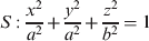
The point P=(x, y, z) on the surface of the unit sphere is usually represented parametrically, using longitude λ and latitude ϕ, as:

where we assume that the equator is the xy-plane and the point (1, 0, 0) is the intersection of the null-meridian with the equator. The coordinates of the point P are also the coordinates of the unit normal of the unit sphere at P. A point P s=(xs,ys,zs) on the spheroid has the unit normal:
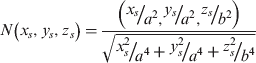
thus, we can parameterize the points of the spheroid; e.g, [Reference Kallay9].
In [Reference Rollins13] a simplified integral is derived for computing the geodesic between two points on a spheroid numerically. The formulation depends on Clairaut's constant that is to be determined, also numerically, before the geodesic can be integrated. Reference [Reference Sjöberg16] proposes a method to compute the constant numerically.
The fact that a numerical computation is needed, coupled with the fact that the eccentricity of the planet is slight, motivates approximating geodesics, and Kallay gives an elegant solution in [Reference Kallay9]. Kallay's construction is as follows: Given two points P 1 and P 2 on the spheroid with normals N 1 and N 2, consider the geodesic between N 1 and N 2 on the Gauss sphere, a greatest circle. Using the inverse Gauss map, this greatest circle is mapped to the spheroid and constitutes the approximate geodesic. Kallay's approximate geodesic can be shown to be a greatest ellipse on the spheroid, that is, the intersection of the spheroid with a plane through the origin; [Reference Kallay9]. This also implies that the approximate geodesic can be extended and that a subdivision of the approximate geodesic is also an approximate geodesic.
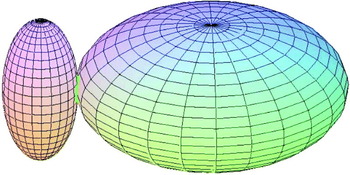
In this paper, we propose an approximation that samples the geodesic circle at four distinguished points and constructs an axis-parallel spheroid that passes through those four points. We note that for approximating circles on an oblate spheroid the intersecting spheroid is prolate, and, conversely, if the circle of a prolate spheroid is to be approximated, then the intersecting spheroid is oblate. The intersection of the oblate spheroid and prolate spheroid then serves as an approximation of the geodesic circle. The approximation is remarkably accurate, even for highly eccentric spheroids.
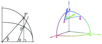
Let P be a point on the spheroid. For its latitude we use the reduced latitude β, as shown in Figure 1 (left). It is related to the geodesic latitude ϕ by:  , where
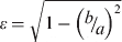 is the eccentricity of the spheroid.
Left: Normal angle ϕ and reduced latitude β. Right: Azimuth α at point P of the geodesic path between two point P and Q.

When following a path from P, the direction in which we head is quantified by α. The angle α is the azimuth of geodesic path at the starting point P. It is the deviation from the meridian through P, with zero the direction to the (north) pole. See also Figure 1 (right). Rollins [Reference Rollins13] presents formulae of proper integrals which solve the direct and indirect problems for geodesic paths connecting two points or azimuth headings.
The Clairaut constant is the cosine of the maximum reduced latitude of a geodesic path,

where α and β are the reduced latitude and azimuth along the geodesic path. Sjoberg [Reference Sjöberg16] gives a numerical method to determine the constant for a geodesic path connecting two given points. He points out that, having determined the constant, accurate relations between the latitude, azimuth and longitude can be computed at any point along the geodesic.
3. APPROXIMATION OF GEODESIC CIRCLES
In this section, we present our approximation of geodesic circles on a spheroid by a Spheroid-Spheroid Intersection (SSI) curve. The geodesic circle on a spheroid S of radius r and centred at the point x0=(x 0,y0,z0)∊S is the set of points x=(x, y, z)∊S such that:

where d g( x, x0) is the geodesic distance between two points x and x0. For each point x on the geodesic circle, there is a geodesic path connecting two points x and x0, which has an azimuth α at the starting point x0, as shown in Figure 1. Thus each point x depends on the heading azimuth α,

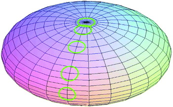
Figure 2 shows the geodesic circles on a spheroid obtained numerically by varying α from 0 to 2π.
Spheroid 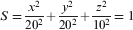 and the five geodesic circles centred at β 0=0°, 30°, 60°, 80° and 90° with geodesic radius=2.

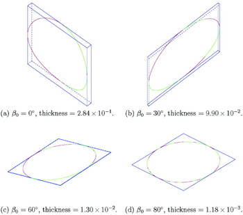
The geodesic circle is not a planar curve unless the centre x0 lies on the North or the South Pole. The two lines x(0)x(π) and  are orthogonal and skew. Thus there are two parallel planes containing the lines. We call the distance between the two parallel planes the thickness of the geodesic circle x(α). Figure 3 shows the parallel planes with a bounding box of the required thickness.
The geodesic circles (green) x(α) and our approximation curves (red) r(z) with the bounding box (blue) for a=20, b=10, and geodesic radius r=2.

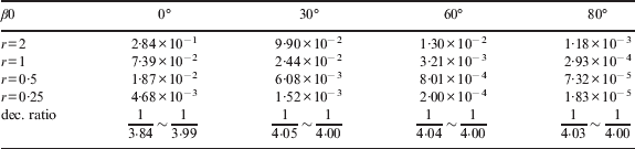
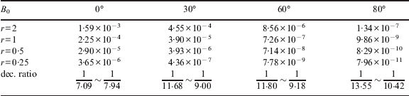
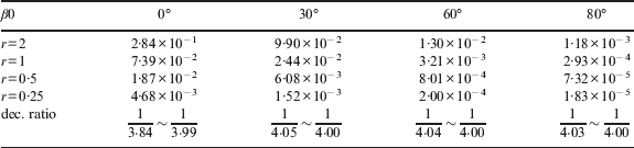
Table 1 shows the thickness of a sample of circles on a spheroid with major axis 20 and minor axis 10. When decreasing the radius of the circle by one half, the thickness decreases to almost 1/4, as shown in the table. The smaller is the radius of geodesic circle, the closer the decreasing ratio is to one quarter.
Thickness of geodesic circles x(α) of radius r=2 centred at β 0 for a=20 and b=10. The last row represents the decreasing ratio of thickness when the radius decreases by half.
In our approximation method, the approximation curve is the intersection of the spheroid S with another spheroid S′ chosen to interpolate the geodesic circle at the points  , where k=0, …, 3; see Figure 2. The new spheroid S′ is centred at x1=(x1,y1,z1) and has the major and minor axes R/a and R/b:
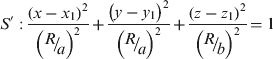
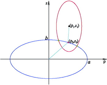
Note that the ratio of the major and minor axes of S′ is inverse of that of S, as shown in Figure 4. Thus, if S is oblate, then S′ is prolate and vice versa. If S is a sphere, then so is S′. Both spheroids S and S′ are symmetric with respect to the plane through the three points, x0, the centre of S′, and the origin. Thus the longitude λ0 of the point x0 is equal to that of the point x1. Cutting the spheroids S and S′ by the ρz-plane of symmetry, two ellipses E and E′ on the ρz-plane are obtained:

where  and
 , i=0, 1, as shown in Figure 5.
The major and minor axes of the prolate (elongated) spheroid S′ are R/a=5·57 and R/b=11·14 when a=20, b=10, β 0=0◦, and r=2.

Two ellipses are the cross-sections of two spheroids S (blue) and S′ (red) with a plane passing through the origin, x0 and the north pole. The geodesic circle x(α) is centred at (ρ 0,z0) and the spheroid S′ is centred at (ρ 1,z1). The two ellipses have intersection points at x(0) and x(π)(green points).

We present the formulae of coefficients of the spheroid S′ as follows:
Proposition 3.1.
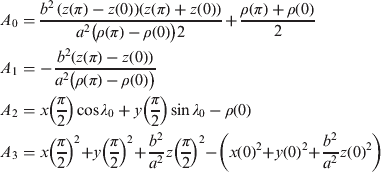
The spheroid S′ in Equation (7) passing through four points,  , k=0, …, 3, is unique unless the geodesic circle is centred at the North or South Pole, and its coefficients are:



where:
Proof.
Let the centre of the geodesic circle lie on the equator, i.e., β 0=0. By symmetry of the geodesic circle with respect to the equator, z 1 and  are zero. Since the ellipse E′ in Equation (8) interpolates the points (ρ(0), z(0)), we obtain Equation (11). Substituting the point x(π/2) into Equation (7) and using:

and Equation (11), we have Equation (10).
Let β 0≠0. Substituting the point (x(0), z(0)) into Equation (8), we obtain Equation (11), and R depends on (ρ 1,z1). Since E′ interpolates two points (ρ(0),z(0)) and (ρ(π),z(π)), Equation (8) yields in this case:

which implies Equation (10), where ρ 1 depends on z 1. Inserting the point x(π/2) into Equation (7) and using Equations (10), (11) and (13), we have:

which is a linear equation of z 1, since ρ 1=A1z1 + A0 is too. Thus it can be solved easily to yield Equation (9). □
The coefficients x 1 and y 1 are obtained by Equation (13) from Proposition 3.1. Table 2 lists the coefficients (R/a, ρ 1,z1) of spheroid S′ for a=20, b=10. Now, the parametric equation of intersection of two spheroids S and S′ can be obtained algebraically, which is our approximation curve for the geodesic circle.
The coefficients (R/a, ρ1,z1) of the spheroid S′ when the geodesic circle centred at β0=0°, 30°, 60°, 80°, with radius r for a=20, b=10.

Proposition 3.2.
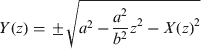
The approximation curve of the geodesic circle is:

for z(π)⩽z⩽z(0), where:

Proof.
Without loss of generality we assume the circle is centred on the 0-meridian. Equivalently, we rotate the axes of x, y by angle λ0 with respect to the z-axis. Let (X,Y,z) be the new coordinates.

Then the spheroids S and S′ in Equations (1) and (7) yield:
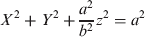

Subtracting Equation (20) from Equation (21) we get Equations (17) and (18). Therefore the assertion follows from Equations (17), (18), and (19), which is the equation for the intersection of two spheroids S and S′. □
Let r(z)=(x(z),y(z),z), for z(π) ⩽ z ⩽ z(0), be our approximation curve. As an example, we approximate several geodesic circles on the spheroid with a=20, b=10. For the geodesic circles x(α) centred at β 0=0° , 30° , 60° and 80°, with the radius r=2, which are shown green in Figure 2, their approximation curves r(z) plotted by red colour together, as shown in Figure 3.
We use the Hausdorff distance d H (x, r) to quantify the maximum difference between two curves x(α) and r(z). The Hausdorff distance is widely used to measure approximation error in Computer Aided Geometric Design, as a fair measure for the distance between two curves or surfaces; e.g., [Reference Ahn1–Reference Barton, Hanniel, Elver and Kim3,Reference Kim, Oh, Yoon, Kim and Elber10]. We sample points along the curves. For the sample points x(α), α=j°, j=0, …, M=180, we calculate the Hausdorff distance numerically by:

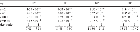
The resulting distance values d H (x, r) for the approximations of the geodesic circles, centred at β 0=0° , 30° , 60°, 80° and with radius r=2, 1, 0·5, 0·25, are shown in Table 3. We observe that the approximation error decreases with ratios between  and
 .
The Hausdorff distance dH (x, r) between the geodesic circle x(α) and our approximation curve r(z) for a=20, b=10.
4. QUALITY OF APPROXIMATION FOR GEOGRAPHIC APPLICATIONS
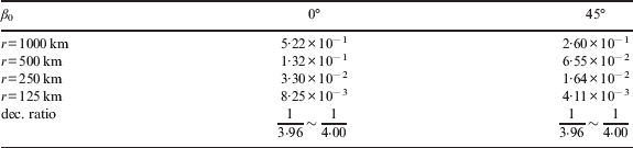
In this section, we use our method to find geodesic circles on the earth's surface. Customarily, the earth is considered an oblate spheroid with axes a=6378·137 km and b=6356·7523 km. We computed the thickness of the geodesic circles of radius r=1000 km, 500 km, 250 km, 125 km, a measure of the non-planarity, shown in Table 4. The decreasing ratios are between  and
 , and the smaller is the radius of geodesic circle, the closer the decreasing ratio is to a quarter, as was the case for the highly eccentric spheroid in Table 1.
Thickness of the geometric circle of radius r=1000 km, 500 km, 250 km, 125 km, and centered at β 0=0°, 45°, on the earth, a=6378·137 km and b=6356·7523 km.
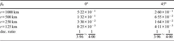
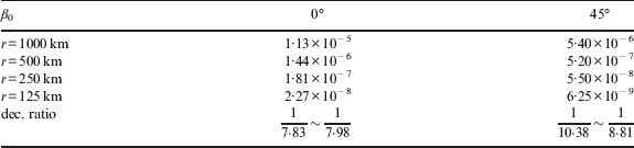
For the geodesic circles centred on the equator (β 0=0°) and with radii r=1000∼ 125 km, the Hausdorff distance measuring the approximation error for our curve r(z) is 1·13 cm or less, as shown in the middle column of Table 5. Also, for the geodesic circle centred at β 0=45°, the Hausdorff distance is 0·54 cm or less, as shown in the third column of Table 5. The approximation accuracy is remarkable.
Hausdorff distance dH (x, r) on the earth (a=6378·137 km and b=6356·7523 km).
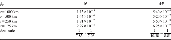
The decreasing error ratios are between  and
 , and the smaller is the radius of the geodesic circle, the closer the decreasing ratio is to
 , similar to the results in Table 3.
To confirm our numerical results, we compute the geodesic distance d g(x0, r(z)) from the approximation curve r(z), z(π)⩽z⩽z(0) to the centre x0. For the sample points:

ζ=(j −0·5)π/M, j=1, …, M, we plot the error function d g(x0, r(ζ)) −r as shown in Figure 6. The fact that the maximum differences  in Table 6 are the almost same as the Hausdorff distances d H (x, r) in Table 5 corroborates the values of Table 6.
On the earth, (a=6378·137 km and b=6356·7523 km), for β 0=0°(left column), 45°(right column), and r=1000, 500, 250, 125 km (from top to bottom), the error function as Equation (23).

The maximum difference  between the radius r and the geodesic distance dg(x0, r(z)) from approximation curve r(z) to the centre x0.

ACKNOWLEDGEMENT
This study was supported by research funds from Chosun University, 2007.