





1. Introduction
Caputo–Fabrizio (CF) and Atangana–Baleanu (AB) fractional models provide a useful framework for studying memory-dependent magnetohydrodynamic (MHD) plasma transport, particularly when magnetic fields, rotation, heating and reactive species are present. However, their practical application to plasma physics requires better physical interpretation of the fractional parameters and validation against real plasma data. Natural or free convection has attracted considerable attention due to its significant role in fluid mechanics, heat transfer and numerous engineering applications. Extensive investigations have been conducted on buoyancy-driven flow and heat transfer characteristics of incompressible, viscous fluids within vertical channels subjected to various thermal boundary conditions. Natural convection governs transport phenomena in a wide range of practical systems, including heat exchangers, thermal management of electronic devices, chemical processing equipment, power generation systems, solar thermal collectors, high-voltage alternating current (HVAC) systems, atmospheric and oceanic circulations, and building thermal regulation. Early investigations into convective heat transfer in channel flows established the theoretical foundation for modern research in fluid dynamics. Ostrach (Reference Ostrach1954) investigated combined natural and forced laminar convection in channels with linearly varying wall temperatures, considering both the presence and absence of internal heat sources, and provided important insights into the underlying heat transfer mechanisms. Bodia & Osterle (Reference Bodia and Osterle1962) subsequently examined the development of free convection between heated vertical plates, advancing the understanding of boundary layer formation and growth. Aung (Reference Aung1972) further extended this work by analysing fully developed laminar free convection between asymmetrically heated vertical plates, demonstrating the influence of unequal wall temperatures on flow and thermal characteristics. Aung & Worku (Reference Aung and Worku1986) later developed a comprehensive theory for fully developed mixed convection, including the prediction of flow reversal under specific operating conditions. Singh (Reference Singh1988) also contributed by investigating natural convection in unsteady Couette flow, highlighting the transient response of fluid motion to time-dependent boundary conditions. Collectively, these pioneering studies provided the fundamental theoretical framework for subsequent investigations of convective heat transfer in vertical channels and related flow configurations. Singh et al. (Reference Singh, Gholami and Soundalgekar1996) investigated transient free convection flow between two vertical parallel plates and provided analytical insights into the time-dependent development of the velocity and temperature fields. Building on this, Paul et al. (Reference Paul, Jha and Singh2001) examined transient natural convection in a vertical channel, further extending the understanding of unsteady thermal flow behaviour. Swarnalathamma et al. (Reference Swarnalathamma, Bharathi and Krishna2026). explored the finite difference simulation of unsteady MHD flow through a non-Darcian porous medium past a vertical cone in geothermal systems. Jha & Ajibade (Reference Jha and Ajibade2009) explored free convective flow of a heat-generating or absorbing fluid between vertical porous plates with periodic heat input, emphasising the role of internal heat generation and absorption on flow characteristics.
Exact analytical solutions were obtained in these investigations. Likewise, Jha & Oyelade (Reference Jha and Oyelade2022) investigated transient free convective flow in a vertical channel using the dual-phase-lag heat conduction model under isoflux and isothermal boundary conditions. Semi-analytical solutions were derived using the Riemann sum approximation technique. Their study demonstrated that both the fluid temperature and velocity were significantly enhanced when the thermal relaxation time was smaller than the thermal retardation time. The incorporation of dynamic and static slip boundary conditions, either individually or simultaneously, plays a vital role in accurately modelling complex transport phenomena encountered in engineering, physical sciences, environmental sciences and biomedical applications. The combined effects of dynamic and static slip provide a better understanding of fluid–wall interactions, momentum transport and thermal transport within channel flows. These slip mechanisms substantially influence the hydrodynamic and thermal boundary layers, thereby improving the prediction of velocity and temperature distributions near the channel walls. Consequently, the inclusion of both static and dynamic slip conditions enhances the physical realism and predictive capability of mathematical models describing fluid motion and heat transfer. Ali et al. (Reference Ali, Ghaleb, Abou-Dina and Helal2023) explored the Laplace transform solution of the time-dependent annular Couette flow with dynamic wall slip. Newtonian plane Couette flow with dynamic slip has been discussed by Abou-Dina et al. (Reference Abou-Dina, Helal, Ghaleb, George and Georgious2020). Jha & Danjuma (Reference Jha and Danjuma2020) investigated the unsteady flow formation in an annulus with partial slippage using a Riemann sum approximation approach. Gbadeyan et al. (Reference Gbadeyan, Abubakar and Oyekunle2020) discussed the effects of Navier slip on a steady flow of an incompressible viscous fluid confined within a spirally enhanced channel. Hamza et al. (Reference Hamza, Bello and Ahmad2023) clearly demonstrated the significant influence of static and dynamic slip boundary conditions on flow and heat transfer characteristics.
Furthermore, heat generation and heat absorption (heat source and heat sink) are fundamental components of the energy equation in the mathematical modelling of heat transfer processes. These terms are widely employed in engineering, industrial, environmental and biomedical applications involving thermal energy transport. Heat generation represents the internal production of thermal energy within the fluid or solid medium and is encountered in applications such as solar thermal collectors, microwave heating, industrial furnaces, electric heaters, boilers, combustion systems and electronic devices. Conversely, heat absorption (heat sink) describes the removal or dissipation of thermal energy from the system, thereby preventing excessive temperature rise and maintaining thermal stability in engineering components and thermal management systems. Heat source and heat sink mechanisms have numerous engineering and technological applications, including thermal management of medical equipment, aircraft cooling systems, industrial machinery, electronic devices and energy conversion systems. The combined effects of internal heat generation and heat absorption are particularly important in heating systems, refrigeration, air-conditioning units, thermoelectric devices, electronic cooling and power generation technologies. Yusuf et al. (Reference Yusuf, Dauda and Adebayo2020) investigated the influence of heat source/sink on MHD start-up natural convective flow in an annulus, considering both isothermal and isoflux boundary conditions, and highlighted its significant impact on thermal and flow characteristics. In a related study, Yusuf & Dauda (Reference Yusuf and Dauda2020) analysed the role of heat source/sink on time-dependent free convective flow in a porous medium confined within a coaxial cylinder, employing a semi-analytical approach to obtain the solutions. Singh & Singh (Reference Singh and Singh2017) examined the effect of heat source/sink on free convective flow of a polar fluid between vertical concentric annuli, demonstrating notable variations in velocity and temperature fields. Similarly, Oni & Jha (Reference Oni and Jha2019) explored heat generation and absorption effects on natural convection flow in a vertical annulus under time-periodic boundary conditions, emphasising the transient behaviour of the system. Jha & Ajibade (Reference Jha and Ajibade2009) studied free convective flow of a heat-generating/absorbing fluid between vertical porous plates with periodic heat input, providing important insights into the influence of internal heat sources on flow development and heat transfer. Their studies demonstrated that heat generation enhances the thermal field by increasing the temperature distribution within the fluid, whereas heat absorption suppresses thermal diffusion and reduces the temperature field throughout the flow domain.
Traditionally, numerous fluid flow and heat transfer problems in engineering, physical sciences and biomedical engineering have been modelled using classical integer-order derivatives. Representative examples include the studies already cited. However, classical constitutive models often fail to accurately describe transport processes involving memory and hereditary effects. Consequently, fractional calculus has emerged as an effective mathematical framework for modelling complex transport phenomena due to its non-local nature and memory characteristics. In particular, the fractional Maxwell model has received considerable attention for describing viscoelastic fluid behaviour and anomalous transport processes with greater accuracy than classical models. To solve the fractional derivative governing equations, many models have been established to manage such a situation. The few among the fractional derivative models are the following. Caputo (Reference Caputo1967) pioneered the concept of fractional derivatives with memory effects by introducing a model of dissipation characterised by nearly frequency-independent behaviour, which laid the foundation for modern fractional calculus in physical systems. Later, Caputo & Fabrizio (Reference Caputo and Fabrizio2015) proposed a novel definition of the fractional derivative with a non-singular kernel, eliminating the limitations associated with classical singular kernels. Building on this advancement, Atangana & Baleanu (Reference Atangana and Baleanu2016) introduced a new class of fractional derivatives with non-local and non-singular kernels, significantly improving the modelling of heat transfer and transport phenomena. Imran et al. (Reference Imran, Akeem, Diaz, Ali and Khan2019) provided a comprehensive analysis of convective flow of fractional MHD viscous fluids using both AB in Caputo sense and CF derivatives under generalised boundary conditions. Similarly, Jha et al. (Reference Jha, Oyelade and Malgwi2022) investigated transient free convection flow between two vertical parallel plates using CF and AB in Caputo fractional time derivatives, employing a semi-analytical approach. Sarwar et al. (Reference Sarwar, Aleem, Asjad and Muhammad2022) extended this framework by incorporating Mittag–Leffler memory into the study of transient free convection flow in a channel, capturing more realistic thermal memory effects. Shah et al. (Reference Shah, Zafar and Fetecau2018) examined free convection flow of a fractional viscous fluid over a vertical plate subjected to shear stress, highlighting the role of fractional parameters in flow behaviour. Furthermore, Abro et al. (Reference Abro, Khan and Tassaddiq2018) applied the Atangana–Baleanu fractional derivative to study MHD convection flow of a Maxwell fluid in a porous medium, while Tassaddiq (Reference Tassaddiq2019) analysed MHD flow of a fractional second-grade fluid over an inclined heated plate. More recently, Saeed et al. (Reference Saeed, Riaz, Baleanu and Abro2020) explored natural convection flow in a channel using non-singular fractional kernels, demonstrating their effectiveness in modelling complex transport phenomena with enhanced physical accuracy.
Laxmaiah & Reddy (Reference Laxmaiah and Reddy2026) investigated the heat and mass transfer characteristics of a Williamson nanofluid over an exponentially permeable stretching surface under MHD conditions. Reddy & Mangamma (Reference Reddy and Mangamma2023) examined the effects of velocity slip and viscous dissipation on MHD heat transfer in Fe3O4–ethylene glycol nanofluid flow over a shrinking sheet in the presence of thermal radiation. Goud & Reddy (Reference Goud and Reddy2026) studied the combined effects of surface permeability and reactive diffusion on magneto-radiative stagnation-point nanofluid flow over a stretching surface. Radhika & Reddy (Reference Radhika and Reddy2025) analysed the effects of thermal radiation on MHD heat transfer in Williamson nanofluid flow over an exponentially porous stretching sheet, incorporating chemical reaction and slip effects. Mangamma et al. (Reference Mangamma, Reddy, Goud, Hendy and Said2024) investigated the influence of velocity and thermal slip on heat transfer in magneto-Casson fluid flow past an exponentially porous stretching surface with chemical reaction and thermal radiation. Reddy & Mangamma (Reference Reddy and Mangamma2024) explored the effects of thermal radiation and chemical reaction on MHD heat transfer in nanofluid flow over a nonlinearly porous stretching sheet with a non-uniform heat source. Goud et al. (Reference Goud and Reddy2024) numerically investigated the dynamics of magnetised Casson fluid flow over a permeable wedge in the presence of viscous dissipation and thermal radiation. Finally, Mangamma & Reddy (Reference Mangamma and Reddy2025) examined the effects of thermal radiation and viscous dissipation on MHD heat transfer in hybrid nanofluid flow over a porous stretching surface. Krishna (Reference Krishna2020) investigated the combined effects of Hall current and ion-slip on radiative MHD rotating flow of Jeffrey fluid past an infinite vertical plate with ramped temperature and velocity boundary conditions. Subsequently, Krishna et al. (Reference Krishna, Ahamad and Chamkha2021) extended this analysis to unsteady laminar free-convective rotating flow of a second-grade fluid over a semi-infinite moving porous surface by considering both Hall and ion-slip effects. More recently, Krishna (Reference Krishna2026) explored the Caputo–Fabrizio fractional model on rotating MHD flow over a vertical porous plate with heat absorption, chemical reaction, Hall and ion slip effects. Ahmad et al. (Reference Ahmad, Ali, Khan, Khan, Alqasem, Elwahab and Omer2025) developed a time-fractional model for MHD slip flow of a viscous fluid in a rotating frame while examining the coupled effects of heat and mass transfer. These studies collectively demonstrate that Hall current significantly modifies the velocity field, alters secondary flow structures and influences momentum, heat and mass transport in electrically conducting fluids subjected to magnetic fields, making it an essential parameter in the analysis of magnetohydrodynamic transport phenomena. Paul et al. (Reference Paul, Jha and Singh1996). explored the transient natural convective flow in a vertical channel with constant temperature and constant heat flux on walls. Kodi et al. (Reference Kodi, Pasha, Algarni, Alqahtani, Rushma and Rameswara Reddy2026) investigated the rotating flow of a hybrid Cu–Al2O3/water nanofluid by incorporating Hall current, Joule heating and nonlinear thermal radiation effects. Using numerical simulations and artificial neural network methods, they demonstrated that these approaches can effectively predict fluid behaviour and heat transfer characteristics. Ravikumar et al. (Reference Ravikumar, Ali, Kodi, Rasool, Turdialiyev, Abduvalieva, Khan and Khedher2026) examined peristaltic blood flow through a tapered channel in the presence of radiative heat flux and chemical reaction effects. Their computational analysis showed that thermal radiation and reaction mechanisms significantly influence biological fluid flows, with important implications for biomedical engineering applications. Similarly, Suneetha et al. (Reference Suneetha, Puvvala and Kodi2026) investigated entropy generation in Carreau–Yasuda hybrid nanofluid flow by incorporating non-Fourier heat flux, couple stress and Soret–Dufour effects. Their findings highlighted the key factors governing energy efficiency in thermal systems. Jyothi et al. (Reference Jyothi, Venkateswarlu, Reddy, Kodi and Damodara Reddy2025) employed neural network techniques to analyse MHD boundary layer flow in Sisko nanofluids, demonstrating that machine learning can improve prediction accuracy for complex fluid-flow problems. In another study, Pasha et al. (Reference Pasha, Al Mesfer, Kareem, Kodi, Danish, Patil and Vaddemani2025) examined unsteady MHD viscoelastic fluid flow through porous media under the influence of rotational forces and thermal diffusion. Their results indicated that these parameters have a significant impact on fluid motion and heat transfer in inclined systems.
Over the past half-century, significant advances have been achieved in the computational treatment of the Navier–Stokes equations through spectral methods, meshless methods, finite-difference methods and finite-element methods. However, in many practical applications, the seamless incorporation of experimental or observational data into existing computational frameworks remains challenging. In addition, mesh generation can be computationally demanding and time-consuming for complex flow configurations. The solution of inverse problems is also often computationally expensive, thereby necessitating the development of novel computational codes and alternative numerical approaches. To address some of these limitations in the modelling of both turbulent and incompressible laminar flows, the present study employs the following mathematical model. None of the aforementioned studies has investigated the effects of a heat source on transient free-convective flow in a vertical channel using CF and AB fractional time derivatives, while simultaneously considering dynamic and static velocity slip conditions with isoflux and isothermal boundary conditions. The novelty of the present study lies in extending the work of Paul et al. (Reference Paul, Jha and Singh1996) by generalising the governing equations through the incorporation of fractional time derivatives with relaxation time in accordance with the fractional Maxwell fluid model and by introducing a heat source term into the energy equation. Furthermore, both dynamic and static slip conditions are imposed as velocity boundary conditions. The primary objective of this study is to obtain semi-analytical solutions for the concentration, temperature and velocity fields by inverting the Laplace-transformed solutions from the Laplace domain to the time domain using the Riemann-sum approximation. This objective is accomplished by employing the CF and AB fractional models together with the method of undetermined coefficients to solve the governing equations. The steady-state solutions for the concentration, temperature, velocity and other relevant physical quantities are also obtained in exact form. Finally, Mathematica 10.4 is employed to investigate the effects of the governing parameters on the obtained solutions through graphical and numerical analyses.
Physical configuration of the problem.

2. Formulation and solution of the problem
We investigated the heat and mass transfer in an infinitely long vertical channel for the unsteady convective rotating flow of a Newtonian viscous fluid through porous medium. The fluid is electrically conducting, and a chemical reaction and heat source are incorporated into the analysis. A schematic representation of the physical flow configuration is illustrated in figure 1. The study considers transient free convection flow of an incompressible, viscous, electrically conducting fluid confined between two infinite vertical parallel plates separated by a distance h. The plates are oriented within the xy-plane, the x-axis is considered to be in the direction of the plates and z-axis is taken normal to it. That is, the x-axis is aligned with the primary flow direction. Both fluid and the plates rotated instantaneously about the z-direction by a uniform angular velocity
 $\Omega$
. An unvarying magnetic field corresponding to the z-direction is provided. At the early stage, when t = 0, the temperature of the fluid and the plate is assumed to be T
0 and no motion is taking place. Subsequently, when
 $t \gt 0$
, the effectiveness of the isoflux heating is anticipated at the position of the plate stationed at z = 0 and isothermal at z = h, and the initial temperature remains the same as T
0. Additionally, the concentrations are preserved as persistent at a quantity C
0. The persistent isoflux and isothermal heating resulted in the convection flow of the fluid. The dynamic and static slips are considered to be responsible for the assumption of the velocity jump at the boundary of the plates. The temperature as well as concentrations quantities near the plate are increased to T
w
and C
w
accordingly. The homogenous chemical reaction occurs among the fluid and diffusing species near an invariable rate Kr. This movement of the velocity, temperature and concentration profiles u, T and C are merely the roles of z and t. By following the perception of the fractional Maxwell fluid model of Laxmaiah & Reddy (Reference Laxmaiah and Reddy2026) and Boussinesq’s estimation, with reference to the work of Swarnalathamma et al. (Reference Swarnalathamma, Bharathi and Krishna2026), the unsteady MHD rotating convection flow of Newtonian viscous fluid through the vertical porous uniform surface is considered. Therefore, the governing equations are modelled as follows:
 \begin{align} \boldsymbol{\nabla }.\,\boldsymbol{V}={0}, \end{align}
 \begin{align} \rho \left(\frac{\partial \boldsymbol{V}}{\partial t}+\left(\boldsymbol{V}.\boldsymbol{\nabla }\right)\boldsymbol{V}+2 \Omega \times \boldsymbol{V}+ \Omega \times \left( \Omega \times \boldsymbol{r}\right)\right)=\mathrm{div}\,\boldsymbol{T} + \boldsymbol{J}\times \boldsymbol{B} + \boldsymbol{R} + \rho \boldsymbol{g}, \end{align}
 \begin{align} \boldsymbol{\nabla }\times \boldsymbol{E} = -\frac{\partial \boldsymbol{B}}{\partial t},\quad \boldsymbol{\nabla }\times \boldsymbol{B} = \mu _{m}\boldsymbol{J},\quad \mathrm{div}\,\boldsymbol{B} = \boldsymbol{0}. \end{align}
The whole strength of the magnetic field is
 $\boldsymbol{B}=B_{0}+b$
, where
 $B_{0}$
is the intensity of the employed magnetic field,
 $b$
the induced magnetic field vector,
 $ \Omega $
the angular velocity and
 $\boldsymbol{r}$
is the radial co-ordinate prearranged by
 $r^{2}=x^{2}+y^{2}$
.
The momentum, energy and concentration equations governing the unsteady MHD free convective rotating flow of a viscous fluid past an unbounded perpendicular porous plate are formulated as follows:
 \begin{align} \frac{\partial u}{\partial x}+\frac{\partial v}{\partial y}=0, \end{align}
 \begin{align} \left(1+{\lambda }_{1}^{\alpha }\frac{\partial ^{\alpha }}{\partial t^{\alpha }}\right)\frac{\partial u}{\partial t}-2 \Omega v & =\nu \frac{\partial ^{2}u}{\partial z^{2}}-\frac{\sigma\kern-2pt {B}_{0}^{2}u}{\rho }-\frac{\nu }{k}u+\left(1+{\lambda }_{1}^{\alpha }\frac{\partial ^{\alpha }}{\partial t^{\alpha }}\right)g\beta (T-T_{0})\nonumber\\[3pt]& \quad +\left(1+{\lambda }_{1}^{\alpha }\frac{\partial ^{\alpha }}{\partial t^{\alpha }}\right)g\beta ^{*}({C}-C_{0}), \end{align}
 \begin{align} \left(1+{\lambda }_{1}^{\alpha }\frac{\partial ^{\alpha }}{\partial t^{\alpha }}\right)\frac{\partial v}{\partial t}+2 \Omega u=\nu \frac{\partial ^{2}v}{\partial z^{2}}-\frac{\sigma \kern-2pt{B}_{0}^{2}v}{\rho }-\frac{\nu }{k}v, \end{align}
 \begin{align} \left(1+{\lambda }_{2}^{\beta }\frac{\partial ^{\beta }}{\partial t^{\beta }}\right)\frac{\partial T}{\partial t}=\frac{k_{1}}{\rho C_{p}}\frac{\partial ^{2}T}{\partial z^{2}}-\frac{Q_{0}}{\rho C_{p}}\left(1+{\lambda }_{2}^{\beta }\frac{\partial ^{\beta }}{\partial t^{\beta }}\right)(T-T_{0}), \end{align}
 \begin{align} \left(1+{\lambda }_{2}^{\beta }\frac{\partial ^{\beta }}{\partial t^{\beta }}\right)\frac{\partial C}{\partial t}=D\frac{\partial ^{2}C}{\partial z^{2}}-{K\!r}\!\left(1+{\lambda }_{2}^{\beta }\frac{\partial ^{\beta }}{\partial t^{\beta }}\right)({C}-C_{0}). \end{align}
The initial and boundary conditions are prescribed as
 \begin{align} u=v=0,\quad\! \frac{\partial u}{\partial t}=\frac{\partial v}{\partial t}=0,\quad\! T=0,\frac{\partial T}{\partial t}=0,\quad\! C=0,\quad\! \frac{\partial C}{\partial t}=0,\quad\!\! t=0,\quad\!\! 0\leq z\leq 1, \end{align}
 \begin{align} u+ \Lambda \frac{\partial u}{\partial t}=\beta _{1}\frac{\partial u}{\partial z},\quad v=0,\quad \frac{\partial T}{\partial z}=-k_{1}\frac{\partial T}{\partial t},\quad \frac{\partial C}{\partial z}=-\frac{\partial C}{\partial t},\quad t\gt 0,\quad z=0, \end{align}
 \begin{align} u+ \Lambda \frac{\partial u}{\partial t}=-\beta _{2}\frac{\partial u}{\partial z},\quad v=0,\quad T=0,\quad C=0,\quad t\gt 0,\quad z=1 .\end{align}
The boundary conditions describe the physical behaviour of the fluid, temperature and concentration at the two walls of the vertical porous channel. If the walls are stationary, the no-slip condition is applied, so the velocity at both walls is zero. The temperatures of the two walls are usually maintained at constant values, which creates a temperature gradient and allows heat transfer through the fluid. Similarly, the concentration of the chemical species at the walls is specified, so the mass diffusion and the effect of the chemical reaction can be studied. These same physical boundary conditions are generally applied in both the CF and AB fractional models. The main difference between the two models is not the physical boundary conditions but the fractional derivative used in the governing momentum, energy and concentration equations. Thus, the boundary conditions ensure that the mathematical solution satisfies the actual physical conditions at the channel walls. Altogether, the physical variables retain their conventional significance. The boundary conditions are imposed based on the assumption that the initial velocity and secondary velocity of the fluid are zero at the plate surface. Far from the plate, the primary velocity approaches the uniform free stream velocity, while the secondary velocity vanishes. The temperature and concentration at the plate are maintained at constant values, and both approach their respective ambient values far from the plate.
Introducing the following non-dimensional quantities:
-
(1)
 $z^{*}=\dfrac{z}{d},\,\,u^{*}=\dfrac{u}{U_{0}},\,v^{*}=\dfrac{v}{U_{0}},\,\,t^{*}=\dfrac{tU_{0}}{d},\,\,\theta =\dfrac{T-T_{0}}{T_{w}-T_{d}},\,\,\phi =\dfrac{C-C_{0}}{C_{w}-C_{d}},$
$\Lambda ^{*}=\dfrac{ \Lambda \nu }{d^{2}},\,\,{\beta }_{1}^{*}=\dfrac{\beta _{1}}{d},\,\,{\beta }_{2}^{*}=\dfrac{\beta _{2}}{d}$
-
(2)
${\textit{Kc}}=\dfrac{\textit{Krd}}{U_{0}},\,M^{2}=\dfrac{\sigma \kern-2pt{B}_{0}^{2}d}{\rho U_{0}},\,K=\dfrac{kU_{0}}{{\rm d}\varphi },\,\,R=\dfrac{ \Omega d}{U_{0}},\,\,{Sc}=\dfrac{\nu }{D},\,\,{\lambda }_{1}^{*}=\dfrac{\lambda _{1}\nu }{d^{2}},$
${\lambda }_{2}^{*}=\dfrac{\lambda _{2}\nu }{d^{2}},$
-
(3)
${\textit{Pr}}=\dfrac{\nu \rho C_{p}}{k_{1}},\,\,\,Q=\dfrac{{\rm d}^{2}Q_{0}}{\mu C_{p}},\,\,{\textit{Gr}}=\dfrac{g\beta d(T_{w}-T_{d})}{{U}_{0}^{2}}\,\,\,\,\mathrm{and}\,\,\,\,{Gm}=\dfrac{g\beta ^{*}d(T_{w}-T_{d})}{{U}_{0}^{2}}.$


Condensing (2.17) and (2.18), and assuming that
 $q=u+iv$
, we obtain (dropping asterisks)
 \begin{align} \left(1+{\lambda }_{1}^{\alpha }\frac{\partial ^{\alpha }}{\partial t^{\alpha }}\right)\frac{\partial q}{\partial t}=\frac{\partial ^{2}q}{\partial z^{2}}+\lambda q+{\textit{Gr}}\!\left(1+{\lambda }_{1}^{\alpha }\frac{\partial ^{\alpha }}{\partial t^{\alpha }}\right)\theta +\textit{Gm}\!\left(1+{\lambda }_{1}^{\alpha }\frac{\partial ^{\alpha }}{\partial t^{\alpha }}\right)\!\phi, \end{align}
 \begin{align} \left(1+{\lambda }_{2}^{\beta }\frac{\partial ^{\beta }}{\partial t^{\beta }}\right)\frac{\partial \theta }{\partial t}=\frac{1}{\textit{Pr}}\frac{\partial ^{2}\theta }{\partial z^{2}}-Q\!\left(1+{\lambda }_{2}^{\beta }\frac{\partial ^{\beta }}{\partial t^{\beta }}\right)\!\theta, \end{align}
 \begin{align} \left(1+{\lambda }_{2}^{\beta }\frac{\partial ^{\beta }}{\partial t^{\beta }}\right)\frac{\partial \phi }{\partial t}=\frac{1}{{Sc}}\frac{\partial ^{2}C}{\partial z^{2}}-{\textit{Kc}}\!\left(1+{\lambda }_{2}^{\beta }\frac{\partial ^{\beta }}{\partial t^{\beta }}\right)\!\phi. \end{align}
The initial and boundary conditions are prescribed as
 \begin{align} q=0,\quad \frac{\partial q}{\partial t}=0,\quad \theta =0,\frac{\partial \theta }{\partial t}=0,\quad \phi =0,\quad \frac{\partial \phi }{\partial t}=0,\quad t=0,\quad 0\leq z\leq 1, \end{align}
 \begin{align} q+ \Lambda \frac{\partial q}{\partial t}=\beta _{1}\frac{\partial q}{\partial z},\quad \frac{\partial \theta }{\partial z}=-\frac{\partial \theta }{\partial t},\quad \frac{\partial \phi }{\partial z}=-\frac{\partial \phi }{\partial t},\quad t\gt 0,\quad z=0 ,\end{align}
 \begin{align} q+ \Lambda \frac{\partial q}{\partial t}=-\beta _{2}\frac{\partial q}{\partial z},\quad \theta =0,\quad \phi =0,\quad t\gt 0,\quad z=1, \end{align}
where
 $\lambda =M^{2}+2iR+({1}/{K})$
.
2.1. Using the Caputo–Fabrizio fractional model
Towards improving the time fractional derivative modelling, we replaced the time derivatives with the CF derivatives in (2.12), (2.13) and (2.14) to yield
 \begin{align} \left(1+\lambda_{1}^{\textit{CF}}{\wp }_{t}^{\alpha }\right)^{\textit{CF}}{\wp }_{t}^{\alpha }q(z,t)=\frac{\partial ^{2}q}{\partial z^{2}}+\lambda q+{\textit{Gr}}\big(1+\lambda _{1}^{\textit{CF}}{\wp }_{t}^{\alpha }\big)\theta +\textit{Gm}\big(1+\lambda _{1}^{\textit{CF}}{\wp }_{t}^{\alpha }\big)\phi ,\end{align}
 \begin{align} \big(1+\lambda _{2}^{\textit{CF}}{\wp }_{t}^{\beta }\big)^{\textit{CF}}{\wp }_{t}^{\beta }\theta (z,t)=\frac{1}{\textit{Pr}}\frac{\partial ^{2}\theta }{\partial z^{2}}-Q\big(1+\lambda _{2}^{\textit{CF}}{\wp }_{t}^{\beta }\big)\theta, \end{align}
 \begin{align} \big(1+\lambda _{2}^{\textit{CF}}{\wp }_{t}^{\beta }\big)^{\textit{CF}}{\wp }_{t}^{\beta }\,\phi (z,t)=\frac{1}{{Sc}}\frac{\partial ^{2}C}{\partial z^{2}}-{\textit{Kc}}\big(1+\lambda _{2}^{\textit{CF}}{\wp }_{t}^{\beta }\big)\phi, \end{align}
where some important definitions are displayed in Appendix A.
After performing the Laplace transforms and using the primary conditions, (2.18), (2.19) and (2.20) are reduced to
 \begin{align} \frac{{\rm d}^{2}\overline{q}}{{\rm d}z^{2}}-m_{1}\overline{q}=-m_{2}\,\overline{\theta }-m_{3}\,\overline{\phi }, \end{align}
 \begin{align} \frac{{\rm d}^{2}\overline{\theta }}{{\rm d}z^{2}}-m_{4}\,\overline{\theta }=0, \end{align}
 \begin{align} \frac{{\rm d}^{2}\overline{\phi }}{{\rm d}z^{2}}-m_{5}\,\overline{\phi }=0. \end{align}
The transformed boundary conditions are
 \begin{align} \overline{q}=\frac{\beta _{1}}{m_{6}}\frac{{\rm d}\overline{u}}{{\rm d}z},\quad \frac{{\rm d}\overline{\theta }}{{\rm d}z}=-\frac{1}{s},\quad \frac{{\rm d}\overline{\phi }}{{\rm d}z}=-\frac{1}{s},\quad \mathrm{at} \ \ z=0, \end{align}
 \begin{align} \overline{q}=\frac{-\beta _{2}}{m_{6}}\frac{{\rm d}\overline{u}}{{\rm d}z},\quad \overline{\theta }=0,\quad \overline{\phi }=0,\quad \mathrm{at} \ \ z=1. \end{align}
Making use of the boundary conditions (2.24) and (2.25), the solutions of (2.21), (2.22) and (2.23) are given by
 \begin{align} \overline{\phi }(z,s)=\frac{\sin (\sqrt{m_{5}}(1-z))}{s\sqrt{m_{5}}\cos (\sqrt{m_{5}})} ,\end{align}
 \begin{align} \overline{\theta }(z,s)=\frac{\sin (\sqrt{m_{4}}(1-z))}{s\sqrt{m_{4}}\cos (\sqrt{m_{4}})} ,\end{align}
 \begin{align} \overline{q}(z,s) & =\left(q_{1}+q_{3}\right)\mathrm{cosh}(\sqrt{m_{1}}z)+\left(q_{2}+q_{4}\right)\mathrm{sinh}(\sqrt{m_{1}}z)\nonumber\\[4pt]& \quad +\frac{m_{2}\sin (\sqrt{m_{4}}(1-z))}{s(m_{1}+M_{4})\sqrt{m_{4}}\cos (\sqrt{m_{4}})}+\frac{m_{3}\sin (\sqrt{m_{5}}(1-z))}{s(m_{1}+m_{5})\sqrt{m_{5}}\cos (\sqrt{m_{5}})}. \end{align}
The transformed solution for the skin friction associated to (2.28) at z = 0 and z = 1 are
 \begin{align} \overline{\tau }_{L}=\left(\frac{{\rm d}\overline{q}}{{\rm d}z}\right)_{z=0}=\sqrt{m_{1}}\left(q_{2}+q_{4}\right)-\frac{m_{2}}{s(m_{1}+m_{4})}-\frac{m_{3}}{s(m_{1}+m_{5})}, \end{align}
 \begin{align} \overline{\tau }_{R} & =\left(\frac{{\rm d}\overline{q}}{{\rm d}z}\right)_{z=1}=-\sqrt{m_{1}}(\left(q_{1}+q_{3}\right)\sinh \sqrt{m_{1}}-\left(q_{2}+q_{4}\right)\mathrm{cosh}\sqrt{m_{1}})\nonumber\\[5pt]& \quad +\frac{m_{2}}{s(m_{1}+m_{4})\cos \sqrt{m_{4}}}+\frac{m_{3}}{s(m_{1}+m_{5})\cos \sqrt{m_{5}}}, \end{align}
where some constants are evaluated and mentioned in Appendix B.
2.2. Using the Atangana–Baleanu (AB) fractional model
Towards improving the time fractional derivative modelling, the time derivatives are replaced with the AB derivatives in (2.12), (2.13) and (2.14) to yield
 \begin{align} \big(1+\lambda_{1}^{AB}{\wp }_{t}^{\alpha }\big)^{AB}{\wp }_{t}^{\alpha }q(z,t)=\frac{\partial ^{2}q}{\partial z^{2}}+\lambda q+{\textit{Gr}}\big(1+\lambda_{1}^{AB}{\wp }_{t}^{\alpha }\big)\theta +\textit{Gm}\big(1+\lambda_{1}^{AB}{\wp }_{t}^{\alpha }\big)\phi ,\end{align}
 \begin{align} \big(1+\lambda_{2}^{AB}{\wp }_{t}^{\beta }\big)^{AB}{\wp }_{t}^{\beta }\theta (z,t)=\frac{1}{\textit{Pr}}\frac{\partial ^{2}\theta }{\partial z^{2}}-Q\big(1+\lambda_{2}^{AB}{\wp }_{t}^{\beta }\big)\theta, \end{align}
 \begin{align} \big(1+\lambda_{2}^{AB}{\wp }_{t}^{\beta }\big)^{AB}{\wp }_{t}^{\beta }\,\phi (z,t)=\frac{1}{{Sc}}\frac{\partial ^{2}C}{\partial z^{2}}-{\textit{Kc}}\big(1+\lambda_{2}^{AB}{\wp }_{t}^{\beta }\big)\phi. \end{align}
After performing the Laplace transforms in addition to using the primary condition, (2.31), (2.32) and (2.33) reduce to
 \begin{align} \frac{{\rm d}^{2}\overline{q}}{{\rm d}z^{2}}-m_{7}\overline{q}=-m_{8}\overline{\theta }-m_{9}\overline{\phi }, \end{align}
 \begin{align} \frac{{\rm d}^{2}\overline{\theta }}{{\rm d}z^{2}}-m_{10}\,\overline{\theta }=0 ,\end{align}
 \begin{align} \frac{{\rm d}^{2}\overline{\phi }}{{\rm d}z^{2}}-m_{11}\,\overline{\phi }=0 .\end{align}
The transformed boundary conditions are
 \begin{align} \overline{q}=\frac{\beta _{1}}{m_{12}}\frac{{\rm d}\overline{u}}{{\rm d}z},\quad \frac{{\rm d}\overline{\theta }}{{\rm d}z}=-\frac{1}{s},\quad \frac{{\rm d}\overline{\phi }}{{\rm d}z}=-\frac{1}{s},\quad \mathrm{at}\quad z=0, \end{align}
 \begin{align} \overline{q}=\frac{-\beta _{2}}{m_{12}}\frac{{\rm d}\overline{u}}{{\rm d}z},\quad \overline{\theta }=0,\quad \overline{\phi }=0,\quad \mathrm{at}\quad z=1. \end{align}
Making use of the boundary conditions (2.37) and (2.38), the solutions of (2.34), (2.35) and (2.36) are given by
 \begin{align} \overline{\phi }(z,s)=\frac{\sin (\sqrt{m_{11}}(1-z))}{s\sqrt{m_{11}}\cos (\sqrt{m_{11}})} ,\end{align}
 \begin{align} \overline{\theta }(z,s)=\frac{\sin (\sqrt{m_{10}}(1-z))}{s\sqrt{m_{10}}\cos (\sqrt{m_{10}})}, \end{align}
 \begin{align} \overline{q}(z,s) & =\left(q_{5}+q_{7}\right)\mathrm{cosh}(\sqrt{m_{7}}z)+\left(q_{6}+q_{8}\right)\mathrm{sinh}(\sqrt{m_{7}}z)\nonumber\\[5pt]& \quad +\frac{m_{8}\sin (\sqrt{m_{10}}(1-z))}{s(m_{7}+m_{10})\sqrt{m_{10}}\cos (\sqrt{m_{10}})}+\frac{m_{9}\sin (\sqrt{m_{11}}(1-z))}{s(m_{7}+m_{11})\sqrt{m_{11}}\cos (\sqrt{m_{11}})}. \end{align}
The transformed solutions for the skin friction associated to (2.41) at z = 0 and z = 1 are
 \begin{align} \overline{\tau }_{L}=\left(\frac{{\rm d}\overline{q}}{{\rm d}z}\right)_{z=0}=\left(q_{6}+q_{8}\right)\sqrt{m_{7}}-\frac{m_{8}}{s(m_{7}+m_{10})}-\frac{m_{9}}{s(m_{7}+m_{11})},\, \end{align}
 \begin{align} \overline{\tau }_{R} & =\left(\frac{{\rm d}\overline{q}}{{\rm d}z}\right)_{z=1}=-\sqrt{m_{7}}((q_{5}+q_{7})\sinh \sqrt{m_{7}}-(q_{6}+q_{8})\mathrm{cosh}\sqrt{m_{7}})\nonumber\\[3pt]& \quad +\frac{m_{8}}{s(m_{7}+m_{10})\cos \sqrt{m_{10}}}+\frac{m_{9}}{s(m_{7}+m_{11})\cos \sqrt{m_{11}}}, \end{align}
where some constants are evaluated and mentioned in Appendix C.
After taking the inverse Laplace transformations, the concentration, temperature and velocity fields using ‘Riemann sum approximation’ are obtained. Also, the steady-state solutions for the concentration, temperature and velocity distributions are derived and are given as
 \begin{align} \phi (z)=\frac{\sin (\sqrt{\textit{ScKc}}(1-z))}{\sqrt{\textit{ScKc}}\cos (\sqrt{\textit{ScKc}})}, \end{align}
 \begin{align} \theta (z)=\frac{\sin \left(\sqrt{\textit{Pr}\,Q}(1-z)\right)}{\sqrt{\textit{Pr}\,Q}\cos \left(\sqrt{\textit{Pr}\,Q}\right)}, \end{align}
 \begin{align} q(z) & =\frac{1}{\left[\textit{Pr}\,Q\right]^{3/2}\cos \left(\sqrt{\textit{Pr}\,Q}\right)}\left(\phi _{1}\left(z+\beta _{1}\right)+\phi _{2}\right)\nonumber\\[4pt]& \quad +\frac{1}{\left[\textit{ScKc}\right]^{3/2}\cos (\sqrt{\textit{ScKc}})}\left(\phi _{3}\left(z+\beta _{1}\right)+\phi _{4}\right)+\cdots\!, \end{align}
where
 $\phi _{1}=({\beta _{2}\sqrt{\textit{Pr}\,Q}+\beta _{1}\sqrt{\textit{Pr}\,Q}\cos \sqrt{\textit{Pr}\,Q}+\sin (\sqrt{\textit{Pr}\,Q})})/({1+\beta _{1}+\beta _{2}});\, \phi _{2}=$
 $\sin (\sqrt{\textit{Pr} \,Q}(1-z))-\beta _{1}\sqrt{\textit{Pr} \,Q}\,\cos \sqrt{\textit{Pr} \,Q}-\sin \sqrt{\textit{Pr} \,Q} ;$
 $\phi _{3}=(\beta _{2}\sqrt{\textit{ScKc}}\,+ \beta _{1}\sqrt{\textit{ScKc}}$
 $\cos \sqrt{\textit{ScKc}}+\sin (\sqrt{\textit{ScKc}}))/({1+\beta _{1}+\beta _{2}});$
 $\phi _{4}=\sin (\sqrt{\textit{ScKc}}(1-z))-\beta _{1}\sqrt{\textit{ScKc}}\,\cos$
 $\sqrt{\textit{ScKc}}-\sin \sqrt{\textit{ScKc}}$
.
The solutions for the skin friction from the velocity at z = 0 and z = 1 are
 \begin{align} \tau _{L} & =\left(\frac{{\rm d}q}{{\rm d}z}\right)_{z=0}=\frac{1}{\left(\textit{Pr}\,Q\right)^{3/2}\cos \sqrt{\textit{Pr}\,Q}}\big[\phi _{1}-\sqrt{\textit{Pr}\,Q}\cos \sqrt{\textit{Pr}\,Q}\big]\nonumber\\[4pt]& \quad +\frac{1}{\big(\textit{ScKc}\big)^{3/2}\cos \sqrt{\textit{ScKc}}}\big[\phi _{3}-\sqrt{\textit{ScKc}}\cos \sqrt{\textit{ScKc}}\big]+\cdots\!, \end{align}
 \begin{align} \tau _{R} & =\left(\frac{{\rm d}q}{{\rm d}z}\right)_{z=1}=\frac{1}{\left(\textit{Pr}\,Q\right)^{3/2}\cos \sqrt{\textit{Pr}\,Q}}\big[{-}\phi _{1}+\sqrt{\textit{Pr}\,Q}\big]\nonumber\\[4pt]& \quad +\frac{1}{\big(\textit{ScKc}\big)^{3/2}\cos \sqrt{\textit{ScKc}}}\big[{-}\phi _{3}+\sqrt{\textit{ScKc}}\big]+\cdots\!. \end{align}
Similarly, the Nusselt number and Sherwood number are attained from temperature and concentration distributions as
 \begin{align} Nu_{L}=-\left(\frac{{\rm d}\theta }{{\rm d}z}\right)_{z=0};\ Nu_{R}=-\left(\frac{{\rm d}\theta }{{\rm d}z}\right)_{z=1};\ Sh_{L}=-\left(\frac{{\rm d}\phi }{{\rm d}z}\right)_{z=0};\ \text{and}\ Sh_{R}=-\left(\frac{{\rm d}\phi }{{\rm d}z}\right)_{z=1}.\nonumber\\[5pt] \end{align}
Here, some terms are not mentioned because of paucity of space.
3. Results and discussion
The present study investigates an unsteady MHD convection flow of a Newtonian gelatinous fluid through bounded perpendicular plates in a gyrating structure with a variable free stream, employing the Laplace transformation method for a comprehensive analysis. A global fractional model based on the Caputo–Fabrizio (CF) and Atangana–Baleanu (AB) approaches are introduced. The solutions for the resultant velocity, including the primary and secondary velocity components, temperature, and concentration distributions, are obtained and presented in figures 2–13. These solutions satisfy the prescribed boundary conditions, as confirmed by tables 1–4. The effects of the governing parameters on the heat and fluid flow distributions in the vertical channel are examined both graphically and numerically using the fractional time derivatives (CF and AB models), dynamic and static slip conditions, and heat source effects. The numerical values are assigned to the appropriate parameters for the precision of the results, otherwise stated, as follows:
 $ M=2, K=1, R=1, \textit{Pr} =0.71$
,
 $ t= 0.2, \alpha = 0.2, \beta =0.2, \textit{Gr} =5 $
,
 $ \textit{Gm} =3,$
 $\textit{Sc} = 0.22, \textit{Kc} =2, \Lambda = 0.1, \beta_1 = \beta_2 = 0.03 $
,
 $ \lambda_1 = \lambda_2= 0.2 $
and
 $ Q = 2 $
.
Velocity profiles against M and K.

Velocity profiles against R and Pr.

When it has been seen at the Hartmann number in figure 2, it tells a classical result, no matter the fractional time CF and AB model and steady-state solution, a bigger Hartmann number (M) still pushes back against the fluid movement. The velocity profiles flatten out and drop, and the boundary layer gets thinner, the Lorentz forces ramp up and slow everything down. Figure 2 also shows how the permeability parameter K, affects the velocity profiles for the CF and AB model, and steady-state solution. When K goes up, both velocity components increase. That is because higher permeability means the fluid faces less resistance as it moves through the porous medium. The fractional time derivatives bring in memory effects, but which do not really change this main trend.
Now, from figure 3 on the CF and AB model and steady-state solutions, the rotation parameter R comes into play. The rotation parameter basically stands for the strength of the Coriolis forces that comes from the system’s rotation. As R increases, the resultant velocity rises throughout the fluid region. These Coriolis forces push the fluid more, especially near the plate. It is noticed that the resultant velocity peaks right next to the plate at high R values, but drops off as it moves away. That is because the Coriolis force is strongest near the plate. The resultant velocity gets a boost near the plate when R is higher, but fades further out. Now, it might to see for the Prandtl number in figure 3. Even in these fractional CF and AB model and steady-state solutions, it acts just like in the classic ones. When Pr goes up, then thermal diffusivity drops. That means lower velocities and a thinner momentum boundary layer are obtained. The fluid just moves less.
Figure 4 on the CF and AB model and steady-state solutions shows how the thermal Grashof number, Gr, changes the velocity profiles. When Gr goes up, the resultant velocity increases because the thermal buoyant forces get stronger. Basically, bigger buoyant forces push the fluid faster, so the fluid moves more and the momentum boundary layer gets thicker. Figure 4 also shows a similiar plot but for the mass Grashof number, Gm. When Gm increases, those concentration buoyant forces pick up and, again, the resultant velocity rise. The fluid moves faster and the boundary layer thickens. This aligns aith what is expected as when Gr or Gm goes up, the buoyant forces, thermal or solutal, start to dominate over the sticky, viscous resistance. These forces show up because temperature or concentration differences make the fluid’s density uneven, and that makes the fluid rise in the warmer or more concentrated regions.
Velocity profiles against Gr and Gm.

Velocity profiles against Q and Kc.

Figure 5 illustrates the effect of the heat source parameter on the resultant velocity for the CF, AB and steady-state models. It is observed that the resultant velocity increases as the heat source parameter increases. This occurs because an increase in the heat source supplies additional thermal energy to the fluid, which raises its temperature and strengthens the thermal buoyancy force. As a result, the fluid motion is enhanced and the resultant velocity increases. In contrast, a heat sink removes thermal energy from the fluid, thereby weakening the buoyancy force and retarding the fluid flow. The figure also shows that the fluid velocity is lower in the time-dependent cases than in the space-dependent case. Furthermore, figure 5 presents the influence of the chemical reaction parameter on the CF, AB and steady-state velocity profiles. As the chemical parameter increases, the resultant velocity decreases. This reduction is associated with the stronger chemical reaction, which modifies and reduces the species concentration and consequently alters the solutal buoyancy force. The weakened buoyancy effect results in a reduction in the overall fluid motion. Thus, the heat source enhances the flow, whereas an increase in the chemical reaction parameter suppresses the resultant velocity.
Through the heat source, the effect of the static slips (
 $ \beta_1, \beta_2 $
) on the CF, AB and steady-state resultant velocity profiles is displayed in figure 6 accordingly. It is observable that the resultant velocity keeps increasing with the increment in the value of
 $ \beta_1 $
. These show that the static slip
 $ \beta_1 $
boost the movement of the fluid. Observably, the resultant velocity of the fluid is pointedly rising towards the plate at z = 0. This indicates that the convection flow of the fluid is more significant at the heat source plate than that of the other. This occurs and aligns with the associated static slip
 $ \beta_1 $
to the position of the plate. Similarly, it is noticeable from the same figures that the resultant velocity increases with the increase of
 $ \beta_2 $
. Apparently, the convection flow is more pronounced at the plate placed at z = 1 than at the plate at z = 0, owing to the influence of
 $ \beta_2 $
. This confirmed the relationship of static slip
 $ \beta_2 $
to the plate at z = 1. Recognisably and from those figures, it is observed that the resultant velocity through the space-dependent region is higher than the velocity produced by the time-dependent region.
Velocity profiles against
 $\beta _{1}$
and
 $\beta _{2}$
.

Velocity profiles against
 $ \Lambda$
and
 $\alpha$
.

Velocity profiles against
 $\lambda _{1}$
and t.

The portrayal of the impact of the varying value of dynamic slip
 $\Lambda$
on the CF and AB velocity components with the heat source is carried out in figure 7. Through the magnification process, it is observed that the velocity gradually declines as the value of
 $\Lambda$
increases. This indicates that the dynamic slip decreased the fluids flow and degraded the convection flow. Again, the impact of the variant value of the fractional order
 $ \alpha $
on the CF, AB and steady-state resultant velocity through the heat source is displayed in the same figure. The resultant velocity from those figures observed decreases with increase in the value of fractional order parameter
 $ \alpha $
. It means that the positive progression in the value of
 $ \alpha $
retards the rising flow of the fluid. This also proves that the higher order of the rate of change of the resultant velocity with respect to time leads to the reduction of convection flow of the fluid. It is observed that the decline in the movement of the fluid, in relation to the increment in
 $ \alpha $
, is more impressive in the case of the heat source than the chemical reaction. This occurs due to the different amounts of heat produced in the process of convection flow through the heat source. Therefore, when the fractional time derivative parameter drops, memory effects get stronger. The resultant velocity profiles exhibit a slower response, which is consistent with the behaviour expected from materials possessing long-lasting memory effects. This behaviour is particularly relevant to complex fluids, viscoelastic materials and porous or absorbent media, in which the present state of the system is influenced by its previous states. The fractional time-derivative parameter provides an effective means of representing these memory effects and allows greater flexibility in describing the fluid’s behaviour. By adjusting this parameter appropriately, the mathematical model can be better aligned with both theoretical predictions and experimental observations.
Figure 8 portrays the influence of the relaxation time parameter
 $ \lambda_1 $
on the obtained CF, AB and steady-state velocity components with respect to the heat source. From both figures, it is observable that the velocity upsurges as the value of
 $ \lambda_1 $
is altered. This establishes that the relaxation time
 $ \lambda_1 $
boosts the movement of the fluid and enhances the convection flow of the fluid. Comparatively, the heat source observable has a more significant impact on the convection flow and the movement of the fluid. Also, an illustration of the obtained resultant velocity via the CF and AB models with the effect of time t is provided in figure 9. From those figures, the resultant velocity increases with the progression of time t. This means that the movement of the fluid is increasingly changing with the variation of time. Apparently, it is noted that the flow of the fluid is considerably greater with the heat source than with the chemical reaction. This indicates that the heat source exceedingly supports the flow of the fluid compared with the heat sink with reverence to time. Separately, it is noticed that the resultant velocity through the CF and AB models reaches the steady state with the heat source when the value of t is higher. Noticeably, it is clear that to see that the CF model produces a greater movement of the fluid than the AB model.
Figure 9 illustrates the effect of the Schmidt number on the resultant velocity profiles for the CF, AB and steady-state models. It is observed that the resultant velocity decreases as the Schmidt number increases. The Schmidt number represents the ratio of momentum diffusivity to mass diffusivity and therefore describes the relative importance of viscous effects and species diffusion in the fluid. When the ratio increases, the mass diffusivity decreases, meaning that the transport of chemical species becomes slower. Consequently, the concentration distribution is reduced, which weakens the solutal buoyancy force responsible for driving the fluid motion. As a result, the fluid movement becomes weaker and the resultant velocity decreases. The reduction in mass diffusion also causes the concentration boundary layer to become thinner. Therefore, an increase in mass diffusion suppresses the resultant velocity and reduces the influence of mass diffusion on the fluid flow.
Velocity profiles against Sc.

Temperature profiles against
 $\beta$
, Pr, Q and t.

Figure 10(a–d) depicts the effects of the variation of fractional order
 $ \beta $
, Prandtl number Pr, Heat source parameter Q and time on the CF, AB and steady-state temperature with the consideration of the heat source, respectively. It is observed from figure 10(a) that the temperature decreases with the increase in the value of
 $ \beta $
. This indicates that the spreading of the heat in the system is completely suppressed with the changes in the value of
 $ \beta $
. Also, this affirms that the distribution of heat becomes less with respect to the high rate of change of the temperature with time. Interestingly, it is observed that the retardation of the temperature is more pronounced in the figure with the heat source than in those with the fractional order
 $ \beta $
. The variation of the Prandtl number Pris shown in figure 10(b) on CF, AB and steady-state solutions. As Pr goes up, heat diffuses more slowly, so the temperature profile drops and the thermal boundary layer gets thinner. A higher Prandtl number just means the fluid does not let heat through very easily, so there is less heat making it into the fluid. When the heat absorption parameter is increased, the fluid temperature falls steadily. Basically, the system is pulling heat out more efficiently, so energy leaves the fluid faster. In thermal physics terms, extracting more energy means the flow cools down, the temperature difference across the region gets smaller and natural convection, that is, buoyancy-driven heat transfer, drops off. A demonstration of the effect of the varying value of the heat source on the CF, AB and steady-state temperature is provided in figure 10(c). It is noticed that the temperature of the CF, AB and steady state increases with the increment of Q. This shows that the propagation of the heat is absolutely enhanced by the heat source. This indicates that, relatively, it can be seen that the heat source generates a huge amount of heat. Apparently, it is noted that the space-dependent temperature is higher than the time-dependent temperature with reference to the heat. Hence, it can be seen that the obtained CF and AB model temperatures increase with the heat source. This shows that the distribution of heat is faster in the case of the heat source than the chemical reaction. Characteristically, the heat source always enhances the spreading of the heat, while the chemical reaction typically opposes the circulation of the heat. Comparatively, it is noted that the CF temperature is higher than the AB model. This is obvious because the AB model has higher memory than the CF model. The steady state for both CF and AB temperature is observed when time is longer. Similarly, the temperature and concentration via CF and AB models attain the steady state more quickly with the chemical reaction than the heat source. The effect of the variation of time t on the CF and AB temperature is depicted in figure 10(d). In the figure, it is clearly observed that the temperature increases as the value of t increases. This implies that the spreading of the heat in the channel is attributed to the increase in time. The thermal boundary layer thickens and diffusion ramps up. Over time, the system settles into a steady state. Hence, given enough time, we will always observe higher temperature profiles, just because the heat has had more time to spread through the fluid.
Concentration profiles against
 $\beta$
, Sc, Kc and t.

Figure 11(a–d) shows how the four factors: fractional-order parameter (
 $ \beta $
), Schmidt number (Sc), chemical reaction parameter (Kc) and time (t) affect the concentration field. The fractional time derivative from the CF and AB models, and steady-state solutions, basically captures how mass diffusion remembers its own past. From figure 11(a), when the fractional order is lower, these memory effects get stronger. The result is that diffusion slows down, and the concentration of the species rises and falls slower over time. So, if we drop the fractional order, lower concentration levels across the whole flow are observed. Now, when we combine stronger chemical reactions with these memory effects, then the concentration drops even more. Fractional-order models really shine here as they can capture all that complicated, intertwined behaviour between reactions and non-local mass transport. Figure 11(b) illustrates the effect of the Schmidt number on the concentration profiles. As the Schmidt number increases, the mass diffusivity decreases, which means that the transport and diffusion of species through the fluid become slower. Consequently, the concentration profile decreases because the chemical species cannot diffuse as effectively into the fluid. This reduction in mass diffusion also causes the solutal concentration boundary layer to become thinner. In contrast, when the Schmidt number decreases, the mass diffusivity increases, allowing the species to spread more rapidly and penetrate farther into the fluid. As a result, the concentration profile increases and the solutal boundary layer becomes thicker. Thus, a higher Schmidt number suppresses mass diffusion and concentration, whereas a lower number enhances both. Figure 11(c) illustrates the effect of the chemical reaction parameter Kc on the concentration profile. The parameter Kc represents the intensity or rate of the chemical reaction occurring within the fluid. As Kc increases, the chemical reaction becomes faster and stronger, causing the chemical species to be consumed more rapidly. Consequently, the concentration of the species decreases within the fluid and, particularly, across the concentration boundary layer. This reduction is more pronounced for a destructive chemical reaction, where the reacting species is continuously consumed by the reaction. Therefore, the concentration profile exhibits a significant decrease as Kc increases, indicating that stronger destructive chemical reactions substantially reduce the availability of the chemical species in the boundary layer. From figure 11(d), as time moves on, species diffuse deeper into the fluid, which bumps up the concentration profiles. The boundary layer gets thicker and the system gradually heads towards a steady state. The longer we wait, the more the mass spreads out, so concentration keeps rising until it levels off.
The consequence of the variation of the relaxation time
 $ \lambda_2 $
on the CF, AB and steady-state temperatures and concentrations is established in figure 12. It is noticed that the temperature is gradually increasing as the value of
 $ \lambda_2 $
increases. It implies that the circulation of heat is greatly supported by the increment in the relaxation parameter
 $ \lambda_2 $
. The immense spreading of heat is highly noticeable through the heat source in relation to the value of
 $ \lambda_2 $
. This shows that the heat source produces a considerably higher temperature. This is also obvious and true due to the ability of the heat source to generate heat in nature. It also reveals the effect of altering the value of the relaxation time parameter
 $ \lambda_2 $
on the CF, AB and steady-state concentration through the justification of the heat source. It is evident to see that the concentration increases with varying the value of
 $ \lambda_2 $
. Outstandingly, it is noticed that the impact of
 $ \lambda_2 $
on the concentration of the fluid is more significant through the heat source.
Temperature and concentration profiles against
 $\lambda _{2}$
.

Stream lines with magnetic field parameter M.

From figures 13 and 14, the rise in the magnetic field parameter M stabilises the streamlines owing to the heightened Lorentz force, which controls fluid movement and retards rotational disturbance within the porous channel. As the fractional parameter enhances in the CF and/or AB fractional modelling, the memory effects became fortified, causing unexpected change in the streamlines structure as well as flow orientations. It is ascertained that the streamlines primarily shift towards the left plate in addition to then instantly back in the primary direction, signifying the strong non-local as well as history dependent natures of the time derivative fractional fluid modelling.
Stream lines with fractional parameter
 $ \alpha $
.

It is noticed from figures 15 and 16, when the magnetic field parameter M enhances, the surface plot shows a reduction in the fluid velocity due to the Lorentz forces, which contends with the fluid movement in addition to the coagulation of the momentum boundary layers. A rise in the chemically reacting parameter Kc retards the concentration distributions since the fortified chemical reaction consumes the species quicker inside the boundary layer. Hence, higher magnetic field strengths suppress the flow nature, whereas higher quantities of Kc heighten the pace of mass transport diminution and concentration decay.
Surface plots with magnetic field parameter M.

Surface plots with chemical reaction parameter Kc.

Heat lines (temperature contours) with heat source parameter Q.

Heat lines (temperature contours) with fractional parameter
 $ \alpha $
.

It is finally noted from figures 17 and 18 that with an enhancement in the temperature resource parameter Q, the temperatures contours become denser and spread more into the fluid regions, signifying increased heat energy creation and a thickened thermal boundary layer. When the fractional parameter
 $ \alpha $
is enhanced, the heat lines exhibit stronger memory and a non-local effect, which modify the temperature organisation and slows the pace of thermal diffusion. Hence, a larger heat resource magnitude increases the fluids temperature, whereas the fractional parameter importantly influences the flow patterns in addition the evolution of temperature transport features.
Shear stresses
 $(\tau )$
at the left plate.

Table 1. Long description
A table with 10 columns and 30 rows. The columns are labeled alpha, M, Pr, Sc, K, R, Kc, Q, Gr, Gm, Lambda, CF model, AB model and Steady state. The table contains numerical values and some blank cells. The values in the CF model, AB model and Steady state columns are given to 6 decimal places. The table shows a variety of data points for different combinations of the other variables.
Shear stresses
 $(\tau )$
at the right plate.

Table 2. Long description
A table with 10 columns and 30 rows. The columns are labeled alpha, M, Pr, Sc, K, R, Kc, Q, Gr, Gm, Lambda, CF model, AB model, and Steady state. The table contains numerical values and some blank cells. The values in the table vary across different rows and columns, with no clear overall trend. All values are approximated.
From tables 1–3, at either of the plates for the CF, AB models and steady states, the shear stress reduces as heat source, dynamic slip and chemically reacting parameters are amplified, whereas it escalates as the values of the fractional derivative parameter, Hartmann number, permeability, rotation, Prandtl and Schmidt numbers, in addition to the thermal and mass Grashof numbers are increased. As might be perceived in table 4, the effects of the fractional time derivative parameter, heat source, Prandtl number and time are analysed. A growing Q results in an improvement of the temperature transports rate, whereas a reducing Q outputs a lessening of the heat transport. The Nusselt number is increasing as the fractional time derivative parameter and heat source are enhanced, and reduces with the relaxation parameter and time. The fractional time derivative parameter, Schmidt number, chemical reaction parameter and time have an impact on the Sherwood number, as displayed in table 4. It is noted that when the fractional time derivative parameter, Sc and Kc upturns, the Sherwood number intensifies, whereas it retards with the relaxation parameter and time.
Nusselt number (Nu).

Table 3. Long description
A table with 7 rows and 8 columns. The columns are labeled beta, Pr, Q, lambda 2, t, CF model, AB model, and Steady state. The table presents numerical values for different parameters and their effects on the CF model, AB model, and steady state. Row 1: beta 0.2, Pr 0.71, Q 2, lambda 2 0.2, t 0.4588968, CF model 0.4255898, AB model 0.3998547. Row 2: beta 0.4, Pr 0.71, Q 2, lambda 2 0.2, t 0.6589958, CF model 0.6211478, AB model 0.5884789. Row 3: beta 0.6, Pr 3.00, Q 2, lambda 2 0.2, t 1.0748996, CF model 0.8440555, AB model 0.7899654. Row 4: beta 0.6, Pr 3.00, Q 7.00, lambda 2 0.2, t 0.7325698, CF model 0.5002145, AB model 0.4778596. Row 5: beta 0.6, Pr 3.00, Q 7.00, lambda 2 1.8, t 1.8100254, CF model 1.7888105, AB model 1.6000354. Row 6: beta 0.6, Pr 3.00, Q 7.00, lambda 2 0.5528954, CF model 0.4857485, AB model 0.4415228. Row 7: beta 0.6, Pr 3.00, Q 7.00, lambda 2 0.6698502, CF model 0.5998547, AB model 0.5587499. Row 8: beta 0.6, Pr 3.00, Q 7.00, lambda 2 0.4332568, CF model 0.4021455, AB model 0.3788596. Row 9: beta 0.6, Pr 3.00, Q 7.00, lambda 2 0.4002578, CF model 0.3887988, AB model 0.3365897. Row 10: beta 0.6, Pr 3.00, Q 7.00, lambda 2 0.4, t 0.4478549, CF model 0.4022599, AB model 0.3714889. Row 11: beta 0.6, Pr 3.00, Q 7.00, lambda 2 0.6, t 0.4345785, CF model 0.3859965, AB model 0.3508547.
Sherwood number (Sh).

Table 4. Long description
A table comparing different models and their parameters for fluid flow analysis. The table has 11 rows and 7 columns. Column headers are Beta, Sc, Kc, Lambda 2, t, CF model, AB model, and Steady state. Row 1: Beta 0.2, Sc 0.71, Kc 1.0, Lambda 2 0.2, t 0.2, CF model 0.859902, AB model 0.7805478, Steady state 0.6550954. Row 2: Beta 0.4, Sc, Kc 1.0, Lambda 2 0.2, t 0.2, CF model 0.998547, AB model 0.8857496, Steady state 0.7885409. Row 3: Beta 0.6, Sc, Kc 1.0, Lambda 2 0.2, t 1.874558, CF model 1.6855479, AB model 1.2254786, Steady state 1.2254786. Row 4: Beta, Sc 3.00, Kc, Lambda 2 0.2, t 1.225478, CF model 1.0024587, AB model 0.9065845, Steady state 0.9065845. Row 5: Beta, Sc 7.00, Kc, Lambda 2 0.2, t 1.569985, CF model 1.2895547, AB model 1.1025448, Steady state 1.1025448. Row 6: Beta 0.2, Sc 2.0, Kc, Lambda 2 0.2, t 1.332568, CF model 1.1258897, AB model 1.0024589, Steady state 1.0024589. Row 7: Beta 0.4, Sc 2.0, Kc, Lambda 2 0.2, t 2.958665, CF model 2.7854458, AB model 2.3369858, Steady state 2.3369858. Row 8: Beta 0.6, Sc 2.0, Kc, Lambda 2 0.2, t 0.685995, CF model 0.6417805, AB model 0.5147855, Steady state 0.5147855. Row 9: Beta 0.2, Sc 3.0, Kc, Lambda 2 0.4, t 0.425899, CF model 0.3906587, AB model 0.2452078, Steady state 0.2452078. Row 10: Beta 0.4, Sc 3.0, Kc, Lambda 2 0.4, t 0.824578, CF model 0.7125895, AB model 0.5547856, Steady state 0.5547856. Row 11: Beta 0.6, Sc 3.0, Kc, Lambda 2 0.4, t 0.778554, CF model 0.6902145, AB model 0.4458778, Steady state 0.4458778.
4. Code validation
Fractional time derivative modelling takes calculus a step further, using derivatives with non-integer orders to dig into how physical systems behave. Ordinary derivatives are not sufficient when it is need to track memory or hereditary effects as they only provide a glimpse of what has happened before. That is where fractional derivatives really shine. They help us understand more complex tasks like visco-elastic materials, diffusion or heat transfer, especially when regular models keep falling short. Engineers, physicists and applied mathematicians rely on these models to make sense of advanced systems. In this study, MATHEMATICA 10.4 is used to simulate how small disturbances move through the system and to calculate velocity distributions under different physical conditions. The results line up almost perfectly with what Paul et al. (Reference Paul, Jha and Singh1996) found earlier (figure 19). This suggests that the numerical code is both accurate and sensitive, and shows excellent promise for future tasks.
Comparison of the results with Paul et al. (Reference Paul, Jha and Singh1996).
 $\alpha =0,$
M = 2, K = 0, R = 0, Kc = 0, Q = 0.5, Gr = 10, Gm = 0, t = 0.2.

5. Conclusions
The investigation of the transient free convection flow in a vertical channel through the application of the CF and AB models with dynamic and static slips has been carried out. The impact of the control parameters on velocity, temperature, concentration, skin friction, Nusselt number and Sherwood numbers has been obtained and elucidated.
-
(1) The resultant velocity decreases with increasing fractional time-derivative parameter and Hartmann number throughout the flow.
-
(2) The thermal buoyancy forces and mass Grashof number enhance the resultant velocity.
-
(3) An increase in the rotation parameter enhances the resultant velocity.
-
(4) Within the boundary layers, the resultant velocity increases with increasing permeability.
-
(5) The temperature decreases with increasing heat absorption and fractional time-derivative parameters.
-
(6) The chemical reaction reduces the species concentration in the fluid as the chemical reaction parameter increases.
-
(7) The heat source enhances the temperature distribution and fluid motion, whereas increasing the fractional time parameter produces the opposite effect.
-
(8) The concentration, temperature, velocity and other relevant physical quantities exhibit higher values for the CF model than for the AB model.
-
(9) The presence of a heat source results in a higher skin-friction coefficient than that produced by the chemical reaction.
-
(10) As the rotation parameter increases, the skin-friction coefficients increase, while the buoyancy forces are also enhanced over time. This, in turn, leads to a reduction in the fluid temperature due to heat absorption.
-
(11) The static slip and relaxation-time parameters promote convective fluid flow, whereas the fractional-order parameters and dynamic slip parameter suppress the upward motion of the fluid.
5.1. Limitations
Despite their usefulness, the CF and AB fractional models have some limitations when applied to plasma physics. First, the choice of the fractional order is often mathematical and may not have a direct physical interpretation unless it is supported by experimental or observational data. The models can also involve assumptions such as incompressible flow, constant material properties, simplified geometry, uniform magnetic fields and simplified chemical reactions, which may not accurately represent real plasma systems. Real plasmas are often highly nonlinear, compressible, turbulent and anisotropic, whereas the simplified channel model may not capture all these effects. In addition, the porous-channel assumption may not represent the complex structure of actual plasma confinement devices. Finally, obtaining analytical or numerical solutions for coupled fractional MHD equations can be computationally demanding, and the results require experimental or simulation-based validation before they can be directly applied to practical plasma systems.
5.2. Applications
This model has several potential applications in plasma physics. It can be used to study magnetised plasma flow in the presence of an externally applied magnetic field, where the Lorentz force influences the velocity and transport characteristics of the plasma. The model is also relevant to plasma confinement and controlled fusion systems, where magnetic fields and rotation are important for controlling plasma motion and temperature. The inclusion of a porous medium can help model plasma interaction with porous or permeable structures, and plasma transport near material surfaces. The heat source is useful for analysing plasma heating, thermal energy generation and temperature distribution, while the chemical reaction term can represent particle production, recombination, ionisation or other species-transport processes in reactive plasma. The fractional CF and AB models are particularly useful when the plasma exhibits memory-dependent or anomalous transport behaviour.
5.3. Future scope
In future research, these models can be extended to more realistic plasma confinement and fusion problems by incorporating non-uniform and time-dependent magnetic fields, variable plasma properties and nonlinear effects. The influence of Hall current, ion-slip effects, thermal radiation, Joule heating, and Soret and Dufour effects can also be included. More advanced models could consider two-phase plasma flow, dusty plasma, nanofluids, micropolar fluids and magnetised reactive plasma. The CF and AB fractional models could also be compared with other fractional operators to determine which model provides a better representation of experimental plasma data. Numerical and computational techniques, together with experimental validation, can further improve the reliability of these models for fusion reactors, plasma processing, astrophysical plasmas and space plasma applications.
Acknowledgements
I would like to thank Dr V.S. Kanchana Bhaskeran, Vice Chancellor of Vellore Institute of Technology University, Vellore, India who helped me in providing high computational software lab fecility and Prof. Khadar Babu SK, Head of the Department has given to me extraordinary support to refine this work.
Editor Roger Blandford thanks the referees for their advice in evaluating this article.
Declaration of interests
The authors report no conflict of interest.
Appendix A
The Caputo–Fabrizio time derivative and is specified as
 \begin{align} ^{\textit{CF}}{\wp }_{t}^{\alpha }q(z,t)=\frac{w(\alpha )}{1-\alpha }{\int }_{0}^{t}\exp\left(\frac{-\alpha (t-\tau )}{1-\alpha }\right)q'\left(z,\,\tau \right)\,{\rm d}\tau ,\quad\alpha \in (0,1) \end{align}
and its Laplace transform is given as
 \begin{align} L\!\left\{^{\textit{CF}}{\wp }_{t}^{\alpha }q(z,t)\right\}=\frac{\textit{sL}\{q(z,t)\}-q(z,0)}{(1-\alpha )s+\alpha }. \end{align}
The Atangana–Baleanu time derivative is specified as
 \begin{align} ^{AB}{\wp }_{t}^{\alpha }q(z,t)=\frac{w(\alpha )}{1-\alpha }{\int }_{b}^{t}E_{\alpha }\!\left(\frac{-\alpha (t-\tau )^{\alpha }}{1-\alpha }\right)q'(z,\tau)\,{\rm d}\tau ,\,\,\,\alpha \in (0,1). \end{align}
Its Laplace transform is given as
 \begin{align} L\!\left\{^{\textit{CF}}{\wp }_{t}^{\alpha }q(z,t)\right\}=\frac{\textit{sL}\{q(z,t)\}-s^{\alpha -1}q(z,0)}{(1-\alpha )s^{\alpha }+\alpha }. \end{align}
 \begin{align} E_{\alpha }\left(-t^{\alpha }\right)=\mathop\sum\limits_{k=0}^{\infty }\left(\frac{-t^{\alpha k}}{ \Gamma (1+\alpha k)}\right) \end{align}
is the Mittag–Lefflers function.
Here,
 $w(\alpha )$
is the normalised function conforming to
 $w(0)=w(\alpha )=1$
and
 $\text{s} \gt 0$
is the Laplace parameter and is specified as
 $L\{q(z,t)\}={\int }_{0}^{\infty }e^{-st}q(z,t)\,{\rm d}t=\overline{q}(z,s)$
.
The inverse Laplace transform of
 $q(z,t)$
can be approximated using Riemann sum based on the Bromwich integral:
 \begin{align} L^{-1}\left\{q(z,s)\right\}=q(z,t)=\frac{e^{\gamma t}}{T}\left(\frac{1}{2}F(\gamma)+ \mathop\sum\limits_{n=1}^{N}\mathrm{Re}\left[F\left(\gamma +\frac{in\pi }{T}\right)e^{in\pi t/T}\right]\right). \end{align}
where
 $\gamma \gt 0$
is a real number chosen to the right of all the singularities of F(s), T is the parameter defining the interval and N is the number of terms.
Appendix B
 \begin{align} m_{1} & =s+\frac{s{\lambda }_{1}^{\alpha }}{\alpha +1-s\alpha }+\lambda ,\,\,m_{2}={\textit{Gr}}\!\left(1+\frac{s{\lambda }_{1}^{\alpha }}{\alpha +s(1-\alpha )}\right),\,m_{3}\nonumber\\[3pt]& =\textit{Gm}\!\left(1+\frac{s{\lambda }_{1}^{\alpha }}{\alpha +s(1-\alpha )}\right), \end{align}
 \begin{align} m_{4}=\textit{Pr} \left(-\left(s+\frac{s{\lambda }_{2}^{\beta }}{\beta +1-s\beta )}\right)+Q\!\left(1+\frac{s{\lambda }_{2}^{\beta }}{\beta +s(1-\beta )}\right)\right), \end{align}
 \begin{align} m_{5}={Sc}\left(-\left(s+\frac{s{\lambda }_{2}^{\beta }}{\beta +1-s\beta )}\right)+{\textit{Kc}}\!\left(1+\frac{s{\lambda }_{2}^{\beta }}{\beta +s(1-\beta )}\right)\right), \end{align}
 \begin{align} m_{6}=1+s \Lambda +s{\lambda }_{1}^{\alpha }\left(\frac{1}{s-s\alpha +\alpha }+\frac{ \Lambda }{1-s\alpha +\alpha }\right). \end{align}
 \begin{align} q_{1} & =\frac{m_{2}}{s\sqrt{m_{4}}(m_{1}+m_{4})\cos (\sqrt{m_{4}})}\nonumber\\[5pt]& \quad \times \left(\frac{d_{1}\left(\begin{array}{l}d_{4}-d_{2}\cos (\sqrt{m_{4}})\cosh (\sqrt{m_{1}})+d_{2}d_{3}\cos (\sqrt{m_{4}})\sinh (\sqrt{m_{1}})\\[5pt]+\sin (\sqrt{m_{4}})\cosh (\sqrt{m_{1}})-d_{3}\sin (\sqrt{m_{4}})\mathrm{sinh}(\sqrt{m_{1}})\end{array}\right)}{\begin{array}{l}d_{1}\mathrm{cosh}(\sqrt{m_{1}})-d_{1}d_{3}\mathrm{sinh}(\sqrt{m_{1}})+\mathrm{sinh}(\sqrt{m_{1}})-d_{3}\cosh (\sqrt{m_{1}})\\[5pt]+\left[d_{2}\cosh (\sqrt{m_{4}})-\sin (\sqrt{m_{4}})\right]\end{array}}\right) ,\end{align}
 \begin{align} q_{2} & =\frac{m_{2}}{s\sqrt{m_{4}}(m_{1}+m_{4})\cos (\sqrt{m_{4}})}\nonumber\\[2pt]& \left(\frac{\left(\begin{array}{l}d_{4}-d_{2}\cos (\sqrt{m_{4}})\cosh (\sqrt{m_{1}})+d_{2}d_{3}\cos (\sqrt{m_{4}})\sinh (\sqrt{m_{1}})\\[2pt]+\sin (\sqrt{m_{4}})\cosh (\sqrt{m_{1}})-d_{3}\sin (\sqrt{m_{4}})\mathrm{sinh}(\sqrt{m_{1}})\end{array}\right)}{d_{1}\mathrm{cosh}(\sqrt{m_{1}})-d_{1}d_{3}\mathrm{sinh}(\sqrt{m_{1}})+\mathrm{sinh}(\sqrt{m_{1}})-d_{3}\cosh (\sqrt{m_{1}})}\right),\end{align}
 \begin{align}q_3 & = \frac{m_3}{s\sqrt{m_5}(m_1+m_5)\cos(\sqrt{m_5})}\nonumber\\[4pt]& \left(\frac{d_5\left(\begin{array}{l}d_8-d_6\cos(\sqrt{m_5})\cosh(\sqrt{m_1}) +d_6d_7\cos(\sqrt{m_5})\sinh(\sqrt{m_1})\\[4pt]+\sin(\sqrt{m_5})\cosh(\sqrt{m_1}) -d_7\sin(\sqrt{m_5})\sinh(\sqrt{m_1})\end{array}\right)}{\begin{array}{l}d_5\cosh(\sqrt{m_1}) -d_5d_7\sinh(\sqrt{m_1})+\sinh(\sqrt{m_1})-d_7\cosh(\sqrt{m_1})\\[4pt]+\,[d_6\cosh(\sqrt{m_5})-\sin(\sqrt{m_5})]\end{array}}\right),\end{align}
 \begin{align}q_4 & = \frac{m_3}{s\sqrt{m_5}(m_1+m_5)\cos(\sqrt{m_5})}\nonumber\\[3pt]& \left(\frac{\left(\begin{array}{l}d_8-d_6\cos(\sqrt{m_5})\cosh(\sqrt{m_1}) + d_6d_7\cos(\sqrt{m_5})\sinh(\sqrt{m_1})\\[4pt]+ \sin(\sqrt{m_5})\cosh(\sqrt{m_1})- d_7\sin(\sqrt{m_5})\sinh(\sqrt{m_1})\end{array}\right)}{d_5\cosh(\sqrt{m_1})-d_5d_7\sinh(\sqrt{m_1})+\sinh(\sqrt{m_1})-d_7\cosh(\sqrt{m_1})}\right)\end{align}
 \begin{align} d_{1}=\frac{\beta _{1}\sqrt{m_{1}}}{m_{6}},\,\,d_{2}=-\frac{\beta _{1}\sqrt{m_{4}}}{m_{6}},\,\,d_{3}=-\frac{\beta _{2}\sqrt{m_{1}}}{m_{6}},\,\,d_{4}=\frac{\beta _{2}\sqrt{m_{4}}}{m_{6}},\, \end{align}
 \begin{align} d_{5}=\frac{\beta _{1}\sqrt{m_{1}}}{m_{6}},\,\,d_{6}=-\frac{\beta _{1}\sqrt{m_{5}}}{m_{6}},\,\,d_{7}=-\frac{\beta _{2}\sqrt{m_{1}}}{m_{6}},\,\,d_{8}=\frac{\beta _{2}\sqrt{m_{5}}}{m_{6}}. \end{align}
Appendix C
 \begin{align} m_{7} & = s+\frac{s^{\alpha }{\lambda }_{1}^{\alpha }}{\alpha +1-\alpha s^{\alpha +1}}+\lambda ,\,\,m_{8}={\textit{Gr}}\!\left(1+\frac{s^{\alpha }{\lambda }_{1}^{\alpha }}{\alpha +s^{\alpha }(1-\alpha )}\right),\nonumber\\[4pt]m_{9} & =\textit{Gm}\!\left(1+\frac{s^{\alpha }{\lambda }_{1}^{\alpha }}{\alpha +s^{\alpha }(1-\alpha )}\right), \end{align}
 \begin{align} m_{10}=\textit{Pr}\!\left(-s\left(1+\frac{s^{\beta }{\lambda }_{2}^{\beta }}{\beta +1-\beta s^{\beta +1}}\right)+Q\!\left(1+\frac{s^{\beta }{\lambda }_{2}^{\beta }}{\beta +s^{\beta }(1-\beta )}\right)\right), \end{align}
 \begin{align} m_{11}={Sc}\!\left(-s\left(1+\frac{s^{\beta }{\lambda }_{2}^{\beta }}{\beta +1-\beta s^{\beta +1}}\right)+{\textit{Kc}}\!\left(1+\frac{s^{\beta }{\lambda }_{2}^{\beta }}{\beta +s^{\beta }(1-\beta )}\right)\right), \end{align}
 \begin{align} m_{12}=1+s \Lambda +s^{\alpha }{\lambda }_{1}^{\alpha }\left(\frac{1}{s^{\alpha }(1-\alpha )+\alpha }+\frac{s \Lambda }{1-\alpha s^{\alpha +1}+\alpha }\right) ,\end{align}
 \begin{align} q_{5} & =\frac{m_{8}}{s\sqrt{m_{10}}(m_{7}+m_{10})\cos (\sqrt{m_{10}})}\nonumber\\[5pt]& \left(\begin{array}{l} \frac{d_{9}\left(\begin{array}{l} d_{12}-d_{10}\cos (\sqrt{m_{10}})\!\cosh (\sqrt{m_{7}})+d_{10}d_{11}\cos (\sqrt{m_{10}})\!\sinh (\sqrt{m_{7}})\\[5pt] + \sin (\sqrt{m_{10}})\!\cosh (\sqrt{m_{7}})-d_{11}\sin (\sqrt{m_{10}})\mathrm{sinh}(\sqrt{m_{7}}) \end{array}\right)} {\begin{array}{l} d_{9}\,\mathrm{cosh}(\sqrt{m_{7}})-d_{9}d_{11}\mathrm{sinh}(\sqrt{m_{7}})+\mathrm{sinh}(\sqrt{m_{7}})-d_{11}\cosh (\sqrt{m_{7}})\\[4pt] +\left[d_{10}\cosh (\sqrt{m_{10}})-\sin (\sqrt{m_{10}})\right]\end{array}} \end{array}\right), \end{align}
 \begin{align}q_6 & =\frac{m_8}{s\sqrt{m_{10}}(m_7+m_{10})\!\cos(\sqrt{m_{10}})}\nonumber\\[4pt]& \left(\frac{\left(\begin{array}{l}d_{12}-d_{10}\cos(\sqrt{m_{10}})\!\cosh(\sqrt{m_7}) + d_{10}d_{11}\cos(\sqrt{m_{10}})\!\sinh(\sqrt{m_7})\\[3pt] + \sin(\sqrt{m_{10}})\!\cosh(\sqrt{m_7}) -d_{11}\sin(\sqrt{m_{10}})\sinh(\sqrt{m_7})\end{array}\right)}{d_9\cosh(\sqrt{m_7})-d_9d_{11}\sinh(\sqrt{m_7})+\sinh(\sqrt{m_7})-d_{11}\cosh(\sqrt{m_7})}\right)\end{align}
 \begin{align}q_7 & = \frac{m_9}{s\sqrt{m_{11}}(m_7+m_{11})\cos(\sqrt{m_{11}})}\nonumber\\[3pt]& \left(\frac{d_{13}\left(\begin{array}{l}d_{16}-d_{14}\cos(\sqrt{m_{11}})\cosh(\sqrt{m_7}) +d_{14}d_{15}\cos(\sqrt{m_{11}})\sinh(\sqrt{m_7}) \\[3pt]+\sin\left(\sqrt{m_{10}}\right)\cosh(\sqrt{m_7})-d_{15}\sin(\sqrt{m_{11}})\sinh(\sqrt{m_7})\end{array}\right)}{\begin{array}{l}d_{13}\cosh(\sqrt{m_7}) -d_{13}d_{15}\sinh(\sqrt{m_7}) +\sin(\sqrt{m_7})-d_{15}\cosh(\sqrt{m_7})\\[5pt]+\,[d_{14}\cosh(\sqrt{m_{11}}) -\sin(\sqrt{m_{11}})]\end{array}}\right)\end{align}
 \begin{align}q_8 & = \frac{m_9}{s\sqrt{m_{11}}\left(m_7+m_{11}\right)\!\cos(\sqrt{m_{11}})}\nonumber\\[4pt]& \left(\frac{\left(\begin{array}{l}d_{16}-d_{14}\cos(\sqrt{m_{11}})\cosh(\sqrt{m_7})+d_{14}d_{15}\cos(\sqrt{m_{11}})\!\sinh(\sqrt{m_7})\\[4pt]+\sin(\sqrt{m_{11}})\!\cosh(\sqrt{m_7})-d_{15}\sin(\sqrt{m_{11}})\!\sinh(\sqrt{m_7})\end{array}\right)}{d_{13}\cosh(\sqrt{m_7}) -d_{13}d_{15}\sinh(\sqrt{m_7}) +\sinh(\sqrt{m_7})-d_{15}\cosh(\sqrt{m_7})}\right)\end{align}
 \begin{align} d_{9}=\frac{\beta _{1}\sqrt{m_{7}}}{m_{12}},\,\,d_{10}=-\frac{\beta _{1}\sqrt{m_{10}}}{m_{12}},\,\,d_{11}=-\frac{\beta _{2}\sqrt{m_{7}}}{m_{12}},\,\,d_{12}=\frac{\beta _{2}\sqrt{m_{10}}}{m_{12}}, \end{align}
 \begin{align} d_{13}=\frac{\beta _{1}\sqrt{m_{7}}}{m_{12}},\,\,d_{14}=-\frac{\beta _{1}\sqrt{m_{11}}}{m_{12}},\,\,d_{15}=-\frac{\beta _{2}\sqrt{m_{7}}}{m_{12}},\,\,d_{16}=\frac{\beta _{2}\sqrt{m_{11}}}{m_{12}}. \end{align}


 β1
 β2

 Λ
 α

 λ1


 β

 β

 λ2


 α


 α
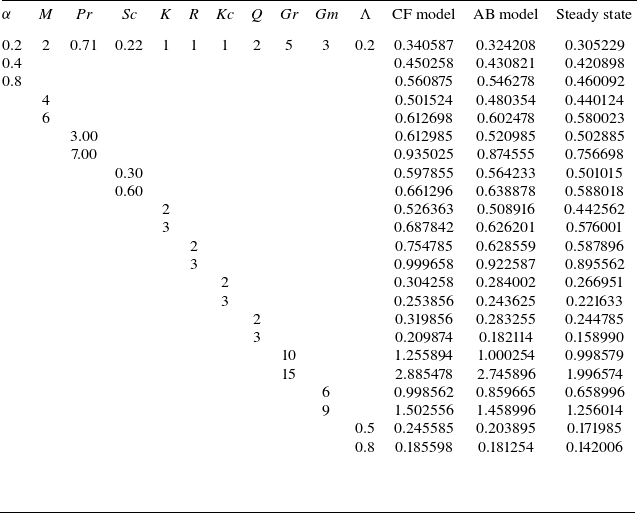
 (τ)
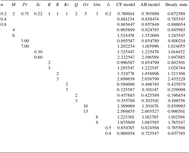
 (τ)
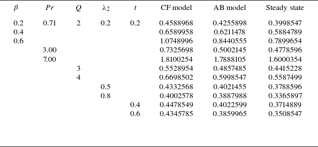
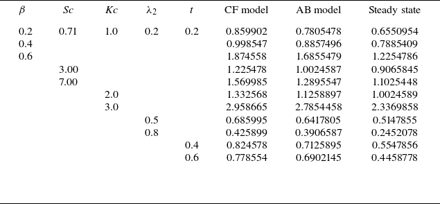
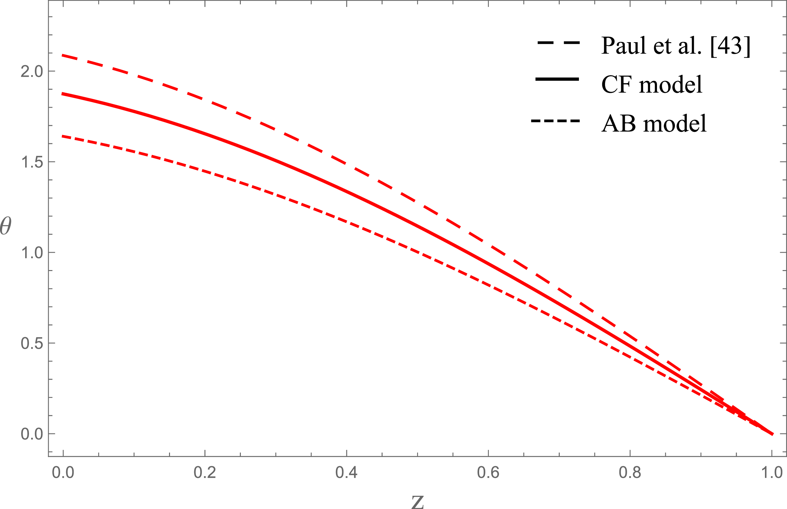
 α=0,

 Open access

