Introduction
Fossil samples from fully lithified sediments can yield depressed estimates of species richness and evenness when compared with samples collected from unlithified sediments (Hendy Reference Hendy2009; Sessa et al. Reference Sessa, Patzkowsky and Bralower2009; Sanders et al. Reference Sanders, Merle and Villier2015). These differences are not a result of larger sample sizes due to the relative ease of specimen collection via sieving unconsolidated sediments in the lab compared with counting specimens on bedding planes, because they cannot be eliminated by correcting for differences in sample size (Hendy Reference Hendy2009; Sessa et al. Reference Sessa, Patzkowsky and Bralower2009). However, the depressed estimates of richness and evenness may be due to the underrepresentation or absence of smaller species: in previous studies comparing fossil samples from lithified and unlithified sediments, samples from lithified rocks tend to be skewed toward larger specimen sizes (Hendy Reference Hendy2009; Sessa et al. Reference Sessa, Patzkowsky and Bralower2009). This effect of lithification state on sampled diversity has been termed the “lithification bias” and is sufficiently large that Hendy (Reference Hendy2011) argued that it represents a megabias with the potential to effect the apparent trajectory of sample-level diversity through the Phanerozoic. Kowalewski et al. (Reference Kowalewski, Wood, Kiessling, Aberhan, Fürsich, Scarponi and Hoffmeister2006) reached a similar conclusion in their analysis of potential sources of bias that could contribute to the apparent post-Paleozoic increase in sample-level diversity. Concerns over the potential for lithification state to bias measures of diversity were significant enough that Alroy et al. (Reference Alroy, Aberhan, Bottjer, Foote, Fürsich, Harries, Hendy, Holland, Ivany and Kiessling2008) excluded collections from unlithified sediments in their sampling standardized analysis of Phanerozoic diversity. Subsequent analyses by Bush and Bambach (Reference Bush and Bambach2015) have raised questions about the degree to which the lithification bias is likely to influence global Phanerozoic diversity trends. However, community-level diversity analyses are still susceptible to this bias, because preferential loss of small specimens can distort rank abundance distributions of species and misrepresent the relative importance of functional groups.
While much attention has been paid to the question of whether lithification state can bias diversity measures, few studies have addressed the question of what mechanism or mechanisms are responsible for this effect, and even less effort has been focused on trying to isolate and test individual mechanisms (see Daley and Bush [Reference Daley and Bush2012] and Nawrot [Reference Nawrot2012] for exceptions). The lithification bias has been largely attributed to preferential dissolution of small aragonitic specimens during early diagenesis (Hendy Reference Hendy2009; Sanders et al. Reference Sanders, Merle and Villier2015), although this mechanism does not seem to have driven a systematic megabias on large-scale evolutionary patterns (Kidwell Reference Kidwell2005). The preferential loss of aragonitic specimens during early diagenesis has been dubbed the “aragonite bias” and has attracted significant attention in the paleobiological literature (Cherns and Wright Reference Cherns and Wright2000, Reference Cherns and Wright2009; Kidwell Reference Kidwell2005; Foote et al. Reference Foote, Crampton, Beu and Nelson2015). However, well-indurated sediments differ from unlithified sediments in other ways besides their diagenetic history. Fossil collection methodologies differ significantly between lithified and unlithified sediments. Unlithified sediments can be sieved in the laboratory, which allows for retrieving all specimens larger than the mesh size from a volume of sediment (Kowalewski and Hoffmeister Reference Kowalewski and Hoffmeister2003). In contrast, fossil collection from lithified sediments or rocks commonly involves (1) counting specimens on naturally exposed bedding planes in the field, (2) counting specimens on mechanically split surfaces in the field or in the laboratory, or (3) extraction of fossils from bulk samples in the laboratory using acid-digestion techniques, although the last method is only applicable in special cases in which fossils are selectively mineralized (e.g., silicified or phosphatized).
Several of the methodological factors involved in sampling lithified sediments could conceivably act as sources of bias. Kowalewski et al. (Reference Kowalewski, Wood, Kiessling, Aberhan, Fürsich, Scarponi and Hoffmeister2006) suggested that breakage and destruction of small specimens during fracturing of lithified rocks could be a source of bias. Additionally, specimens collected from even partially lithified sediments often cannot be fully separated from the enclosing matrix, leading to the loss of taxonomically diagnostic features (Hendy Reference Hendy2009). If some taxa are more easily identifiable based on fragments or partially exposed specimens, then the “Chlamys effect” (Kowalewski et al. Reference Kowalewski, Carroll, Casazza, Gupta, Hannisdal, Hendy, Richard, LaBarbera, Lazo and Messina2003)—specimens that can be more easily identified as fragments are overrepresented—can lead to a bias. In some cases, biases may have both methodological and diagenetic components. For example, fossils of different diagenetic histories and preservational states (e.g., full shells vs. molds) can influence the ease of specimen collection and taxonomic identification.
Even without specimen destruction or biased identification, sampling methods for well-lithified sediments have the potential to result in a size-related bias. This is because the collection methods noted above, with the exception of acid digestion which is only applicable to rare cases of selectively mineralized fossil assemblages, are limited to sampling only those specimens intersected by natural outcrops or artificially split surfaces. Given that larger specimens are more likely than smaller specimens to be intersected by such surfaces, it is conceivable that this could also lead to its own size-related bias. This phenomenon of size bias related to intersection has previously been recognized in contexts ranging from paleobiology to igneous petrology (McKinney Reference McKinney1986; Peterson Reference Peterson1996) but has not been previously considered as a potential mechanism for the lithification bias. We term this mechanism “preferential intersection.”
Here we use a simple analogue model to simulate fossil collection from lithified sediments in order to test the hypothesis that preferential intersection can bias assemblage richness, evenness, and average specimen size. The model, implemented in Matlab, evaluates how various factors such as species abundance distribution, size differences among species, and fossil density affect the degree to which preferential intersection can bias the diversity of fossil samples. By determining how much bias can be generated independent of dissolution of aragonitic specimens, mechanical destruction of small specimens, and biased identification, we place constraints on the degree of species loss due to these mechanisms that must be invoked in order to explain the empirically demonstrated lithification bias. Finally, we consider factors that the model does not address and how these may contribute to the lithification bias.
Methods
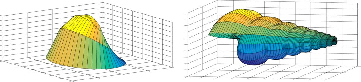
To explore the impact of preferential intersection on paleobiological sampling, we developed a simple model that captures the basic aspects of fossil sampling from lithified rock. Here we describe the basic parts of the model and how it was used to investigate the biasing effects of preferential intersection. A more detailed description of the model is provided in Supplementary Appendix I. The model in its simplest form consists of three components: a cube of a given volume, one or more fracture planes intersecting the cube, and specimens populating the cube. Each of these components was represented in Matlab as sets of three-dimensional coordinates. For cubic volumes and fracture planes, this was straightforward. Sets of coordinates for the more geometrically complex specimens were generated using Raup’s (Reference Raup1966) coiling model (Fig. 1). The populated volume is analogous to a fossiliferous rock and is sampled by being bisected by one or more horizontal planes, analogous to planar fractures or bedding surfaces, at random points along its vertical axis. Specimens intersected by one or more planes were considered exposed and were counted.
Examples of a bivalve (left; a single valve) and a gastropod (right) generated using Matlab code that implemented Raup’s (Reference Raup1966) coiling model.

Model Parameterization and Sources of Data
For the model to be able to populate cubic volumes with realistic multispecies assemblages, we first created nine parent populations of shells from which specimens could be drawn at random. The nine parent populations represented different combinations of three species abundance distributions and three sources of species size data, which are described below. Each parent population contained 1,000,000 specimens to ensure an adequate sampling universe. In each parent population, specimens were distributed among species according to one of three species abundance distributions. Each species was assigned a size value, status as a gastropod or bivalve, and shell shape data. Two separate sets of shape data, one for shells assigned as gastropods and the other for shells assigned as bivalves, were used to avoid assigning unrealistic shapes. For simplicity, each species was defined by a distinct but uniform size and shape (i.e., there were interspecific variations in size and shape, but there were no intraspecific variations). The model used one shell dimension (i.e., shell height or distance from the dorsal to the ventral sides of the shell) as a measure of size.
Data on species abundances are commonly presented in the paleoecological literature; however, these are usually limited to samples of only a few hundred or at best thousands of individuals. Therefore, to have a sampling universe sufficient to explore variation in diversity up to sample sizes of thousands of individuals, we chose to generate artificial data sets of size N=1,000,000 based on realistic parameters. To do this, we used three species abundance distributions: two following the log-series distribution (Fisher et al. Reference Fisher, Corbet and Williams1943) and one following the lognormal distribution (Bulmer Reference Bulmer1974). Parameter values for the species abundance distributions were α=3 and α=6 for the two log-series distributions, and μ=1.2281 and σ=1.240 for the lognormal distribution. A detailed description of how these species abundance distributions were generated is presented in Supplementary Appendix I. Matlab codes for this and other procedures are included in the Supplementary Data.
Three sources of size data (Roy et al. Reference Roy, Jablonski and Martien2000; Kowalewski and Hoffmeister Reference Kowalewski and Hoffmeister2003; Sessa et al. Reference Sessa, Patzkowsky and Bralower2009) formed the basis for constructing the parent populations with varying size between model species. The supplementary data set of Kowalewski and Hoffmeister (Reference Kowalewski and Hoffmeister2003) provided lists of specimens identified to species level with associated measurements of shell height. The mean of individual species provided a basis for a data set of species sizes. Roy et al. (Reference Roy, Jablonski and Martien2000) provided numbers of species assigned to different size bins. Sessa et al. (Reference Sessa, Patzkowsky and Bralower2009) provided lists of species taken from both their own work and previously published sources. While Sessa et al. (Reference Sessa, Patzkowsky and Bralower2009) did not provide species size information, one of their sources of species abundance data, Garvie (Reference Garvie1996), gave species-level size information including shell heights, width:height ratios, and length:height ratios. Measurements were given for the largest specimen of a species. This information was used as a source of size information for the species lists of Sessa et al. (Reference Sessa, Patzkowsky and Bralower2009). Details of the treatment of size data, including a discussion of different binning methods used in the three data sets, are included in Supplementary Appendix I. In contrast to specimen size, where we used three data sets to explore the effect of species size, only a single data set on shell shape was used for all analyses. Details of how shape data were used are described in Supplementary Appendix I. Shape data used in the model were taken from two sources, the Paleobiology Database and Garvie (Reference Garvie1996). Shape data were obtained for species lists of Sessa et al. (Reference Sessa, Patzkowsky and Bralower2009) to ensure that the range of within-population shapes was realistic. Assignment of a size value to a species was random with respect to the species abundance value assigned to that species, such that a species was as likely to be assigned a larger or smaller size value regardless of whether it occurred rarely or abundantly in the parent population. This represents a simplification of the model, because in reality species size and abundance may be related, for example, smaller taxa tend to be highly abundant (Warwick and Clarke Reference Warwick and Clarke1996).
The Model
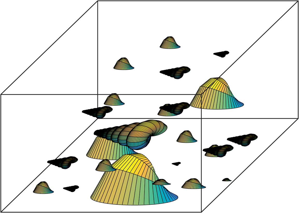
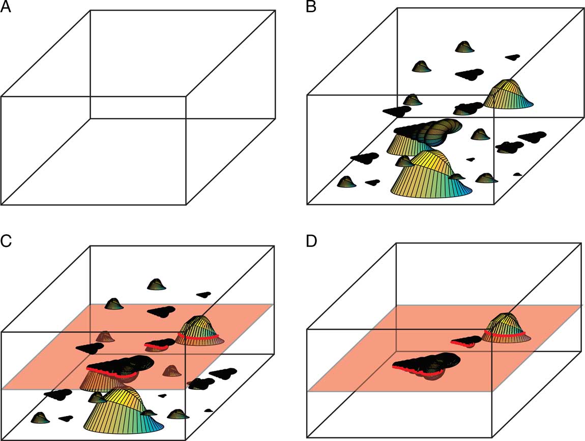
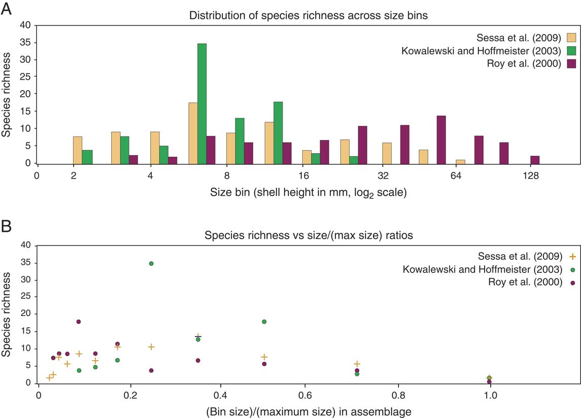
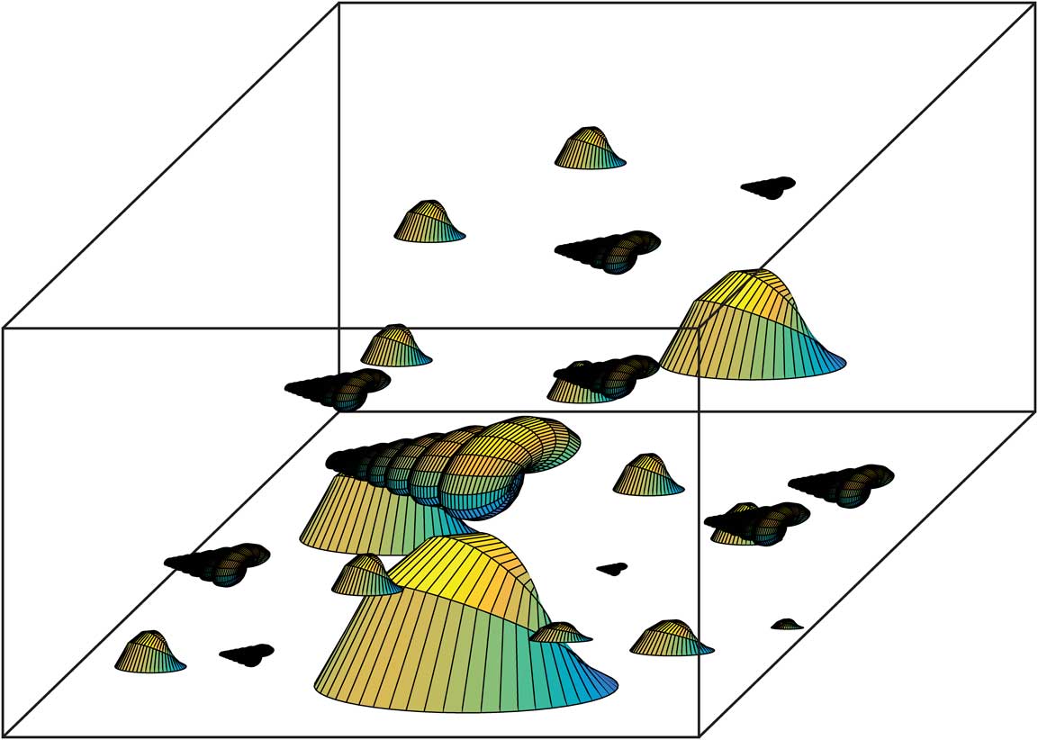
Once generated from the compiled data, the nine parent populations could then be drawn from to populate model rock volumes. Model rock volumes were populated by randomly drawing specimens, without replacement, from the parent distribution and then randomly placing them in the rock volume (Figs. 2 and 3B). When placed in the model volume, all specimens are oriented so that the dorsoventral axis in bivalves and the anterior–posterior axis (or the aperture–apex axis) in gastropods is parallel to the “bedding plane” of the populated volume. The bivalve and gastropod shells created using the Raup model served as the basis for generating specimens of different species that varied in shape. These baseline model shells each possess shell height, width, and length values of 1 mm. Therefore, to generate a specimen of a particular size, the baseline set of coordinates were linearly scaled so that the specimen had a shell height equal to the size-bin value assigned to its species. For simplicity, we chose to associate each species with only a single size value and ignored intraspecific size variation. The assignment of a single size category to all members of a species is obviously a simplification, as in reality specimens would exhibit size variation based on ontogenetic stage and other factors. This simplification is partly justified, because the goal of this study is to understand the effect of preferential intersection on species-level size distribution rather than intraspecific size distribution. The single size assigned to a species in the present model can be thought of as equivalent to the mean shell height of this species. Indeed, this size was taken from the mean shell size for each species reported in the Kowalewski and Hoffmeister (Reference Kowalewski and Hoffmeister2003) data set. As the mean size measurements were not reported in the two other sources of size distribution, the species size in our model was taken from the largest available specimen of each species reported in Roy et al. (Reference Roy, Jablonski and Martien2000) and the largest specimen size from Garvie (1996). Nevertheless, the comparison of the different species-level size distributions is useful in assessing how they can influence the effect of preferential intersection. Figure 4 shows the distribution of species among size categories for each of the three size distributions.
An example of a populated volume. The number of specimens placed within each volume was defined by the user and was limited by the requirement that specimens cannot penetrate one another.
The stages of model population and sampling. A, An initial volume was defined based on user-defined size parameters. B, This volume was then populated by specimens randomly drawn from a parent distribution. This was an iterative process that began with drawing, without replacement, a set number of specimens from the parent distribution. The specimens were then placed in the volume sequentially in order of decreasing size. Each newly placed specimen was assessed to determine whether it penetrated any previously placed specimens. If it did, then it was randomly assigned a new location until it did not penetrate any existing specimens. C, One or more horizontal planes within the volume were randomly selected to represent fracture surfaces that intersected specimens. D, Finally, the species identity and size of each intersected specimen were stored in a master list. If the user-defined sampling quota had not been reached, a new populated volume was generated and the procedure was repeated until the quota was met.

The three size distributions (Roy et al. Reference Roy, Jablonski and Martien2000; Kowalewski and Hoffmeister Reference Kowalewski and Hoffmeister2003; Sessa et al. Reference Sessa, Patzkowsky and Bralower2009) used in the model. A, Plotted in absolute size bins. B, The same data plotted in relative size bins (i.e., fraction of the largest bin).

Specimen shape was modified by the model in association with size modification. While the shell heights were scaled only by the size value, the shell lengths and widths were scaled additionally by the length or width aspect ratios, respectively. Again, for simplicity, each species was associated with only a single shape, and intraspecific shape variation was ignored.
Specimens were assigned random locations within the cubic volume one at a time in order of decreasing size. The model assessed whether each newly placed specimen intersected any previously placed specimen, and if intersection was detected, location assignment was repeated until no specimen intersection occurred. Details of how the model handled assessing specimen intersection are presented in Supplementary Appendix I.
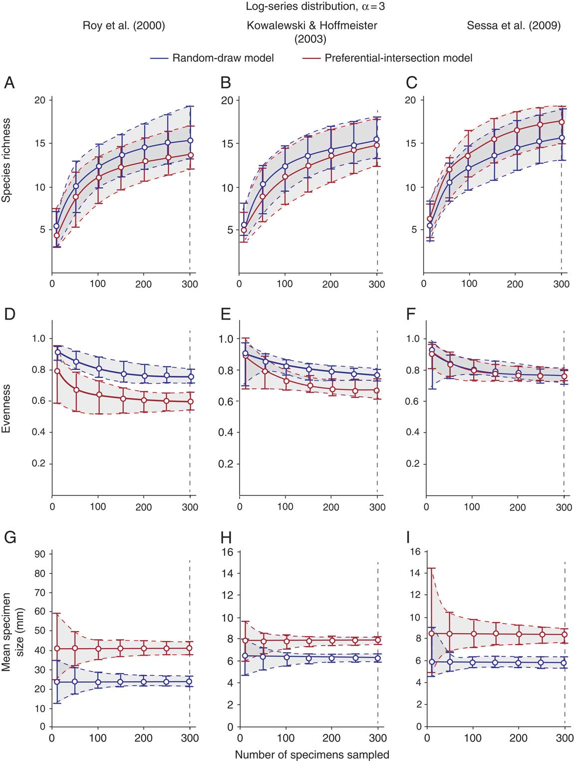
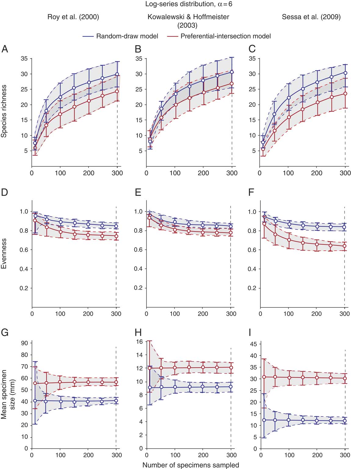
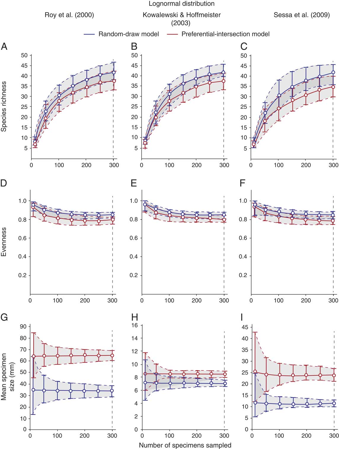
Once a volume was populated by specimens, one or more positions along the vertical axis between the top and bottom of the volume were selected at random (Fig. 3C). These points represent fracture horizons or bedding surfaces. All specimens intersected by one or more of these horizons were counted by the program, and their species identity and associated information recorded. The program recorded information about each intersected specimen, including its species identity and size, and stored this information in a master list of sampled specimens. The program continued to generate and sample populated volumes until a user-supplied sample-size quota was met. This quota represents the sampling intensity and is represented in the horizontal axis in Figures 5–7. In different model runs, the quotas were set at 10, 50, 100, 150, 200, 250, and 300 specimens, allowing us to examine the effects of different sampling intensities on the magnitude of bias induced by preferential intersection. Intuitively, as the sampling intensity approaches infinity, the model would exhaustively sample every specimen in the volume and thus capture all specimens present in the sampled unit.
Results of model runs using all three size distributions and a log-series species abundance distribution with α=3. Circles and brackets represent the mean values and 95% confidence intervals.

Results of model runs using all three size distributions and a log-series species abundance distribution with α=6. Circles and brackets represent the mean values and 95% confidence intervals.

Results of model runs using all three size distributions and a lognormal species abundance distribution (μ=1.2281, σ=1.2408). Circles and brackets represent the mean values and 95% confidence intervals.

Considering all intersected specimens as equally exposed is another simplification in our model, given that, in reality, fragments of a specimen may or may not be taxonomically identifiable. This is analogous to the Chlamys effect of Kowalewski et al. (Reference Kowalewski, Carroll, Casazza, Gupta, Hannisdal, Hendy, Richard, LaBarbera, Lazo and Messina2003), who have demonstrated that some taxa such as Chlamys are more readily identifiable from fragments than others. However, this simplification is a conservative measure because the Chlamys effect tends to depress diversity and evenness (Kowalewski et al. Reference Kowalewski, Carroll, Casazza, Gupta, Hannisdal, Hendy, Richard, LaBarbera, Lazo and Messina2003), and thus, in reality, preferential intersection would impart a greater bias than modeled here.
Rock fracture is also treated in a simplified fashion in the model. In reality, the path of a fracture is influenced by mechanical weakness, including the interfaces between shells and surrounding matrix or, alternatively, the existence of moldic fossils. Because larger fossils represent larger areas of weakness, fractures would be expected to preferentially occur along the interface between them and the rock matrix (i.e., fractures preferentially “find” these larger fossils). In the model, fractures are treated simply as planar features that are not influenced by mechanical weakness at fossil–matrix interfaces. This treatment of fractures is conservative with respective to average specimen sizes.
Once the quota was reached, the resulting sample was used to calculate the species richness, evenness, and average specimen size of the sample. Evenness was calculated as Pielou’s J (Pielou Reference Pielou1966). Average specimen size was estimated as arithmetic mean of all specimens captured in a sample regardless of species identity. The procedure was then repeated 150 times. Mean values and 95% confidence intervals for species richness, evenness, and mean specimen size were then calculated based on the range of values yielded over these 150 model iterations. The small number of iterations reflects practical constraints of this computationally intensive model. Several model runs were repeated multiple times to confirm that the model produced consistent results with 150 iterations.
As a null model, samples were generated by randomly drawing specimens, without replacement, from the same parent populations used to populate the model volumes. This model is analogous to fossil collection by sieving unconsolidated sediments and retrieving all specimens contained within a given volume of sediments. Results from the random-draw simulation are compared with those from the preferential-intersection simulation at the same sampling intensities (n=10, 50, 100, 150, 200, 250, and 300). Intuitively, as the sampling intensity approaches infinity, and in particular as the number of splitting planes per volume increases, the two simulations should yield converging results. In reality, however, sampling is never exhaustive. Thus, our simulations mimicked sampling intensities and splitting-plane densities that typify empirical studies.
A potential criticism of using the random-draw model to simulate fossil sieving is that sieving is itself a nonrandom collection method. Fossil collection via sieving invariably fails to sample specimens smaller than the mesh size. As a result, a pure random-draw model would not accurately recreate the act of fossil sieving if it collects specimens smaller than the mesh size. However, the fossils in our models are larger than 2 mm in shell height (Fig. 4), and several empirical studies used for comparison with model results also employed sieves with 2 mm mesh size (Sessa Reference Sessa2009; Sessa et al. Reference Sessa, Patzkowsky and Bralower2009; Nawrot Reference Nawrot2012). Thus, it is appropriate to use the random-draw model to approximate fossil sieving as long as mesh size is kept at 2 mm. Fossil sieving could also be affected by other biases (e.g., breakage of extremely fragile specimens) that are not captured by the random-draw model, but it is reasonable to assume that such biases are relatively minor compared with those associated with sampling lithified sediments. Thus, a random-draw model can be and indeed has previously been used to model fossil collection via sieving (Kowalewski and Hoffmeister Reference Kowalewski and Hoffmeister2003). Like the preferential-intersection model, the random-draw model was repeated 150 times for each quota size to calculate the mean and 95% confidence interval of species richness, evenness, and average specimen size.
The nine parent populations described above provided a basis for assessing how the magnitude of bias induced by preferential intersection varied in response to changes in the species abundance and size distributions. Each parent population was run through both the preferential-intersection and random-draw models. The resulting curves of mean values and confidence intervals for species richness, assemblage evenness, and average specimen size allowed us to examine how the magnitude of the bias changed with sampling intensity for each combination of species abundance and size distributions. We also performed two-tailed t-tests on sets of 150 values produced by the preferential-intersection and random-draw models, at a sample-size quota of 300 specimens, to determine whether one of the two models produced significantly higher or lower richness, evenness, and average specimen size.
To investigate the impact of per volume splitting intensity on the magnitude of bias, we ran the preferential-intersection model with the Roy et al. (Reference Roy, Jablonski and Martien2000) species size distribution and the lognormal species abundance distribution (μ=1.2281, σ=1.2408, and total species richness=50), with the quota fixed at 100 specimens. We ran the model with per volume splitting intensity at 1, 5, 10, 15, 20, and 25. As above, each model run was repeated 150 times to generate a mean and the 95% confidence intervals. A more detailed description is provided in Supplementary Appendix II.
Results
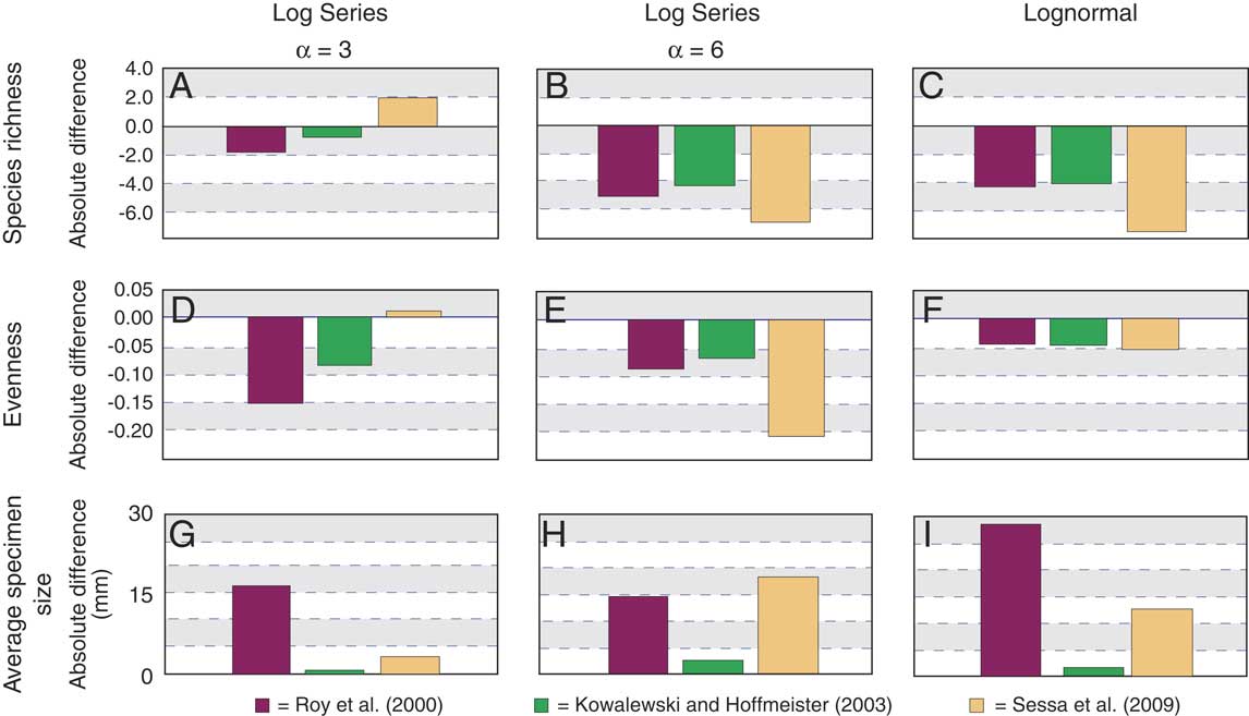
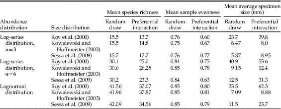
Examination of the results produced by the two models (Figs. 5–9, Table 1) demonstrates that all model runs show some degree of difference in species richness, evenness, and/or average specimen size between samples produced by the preferential-intersection and random-draw models. However, the magnitude of this difference, and to a lesser extent the direction (i.e., whether the preferential-intersection model yielded greater or lower species richness, evenness, or average specimen size than did the random-draw model), varied among model runs that used different combinations of the species abundance and size distributions. In the following sections, we briefly summarize the differences between samples produced by the random-draw and preferential-intersection models for a sampling intensity of n=300 (Fig. 8). To show the percentage differences between the two models, we also normalized these differences against results from the random-draw model (Fig. 9). We also report the results of two-tailed t-tests comparing the species richness, evenness, and average specimen size produced by the preferential-intersection and random-draw models at a sample quota of 300 specimens and across 150 iterations (Table 2).
Absolute differences in mean species richness, evenness, and specimen size between the preferential-intersection and random-draw models, produced in nine combinations of three species abundance distributions (log series α=3; log series α=6; lognormal μ=1.2281, σ=1.2408) and three size distributions (Roy et al. Reference Roy, Jablonski and Martien2000; Kowalewski and Hoffmeister Reference Kowalewski and Hoffmeister2003; Sessa et al. Reference Sessa, Patzkowsky and Bralower2009). The differences are displayed as preferential-intersection value – random-draw value.

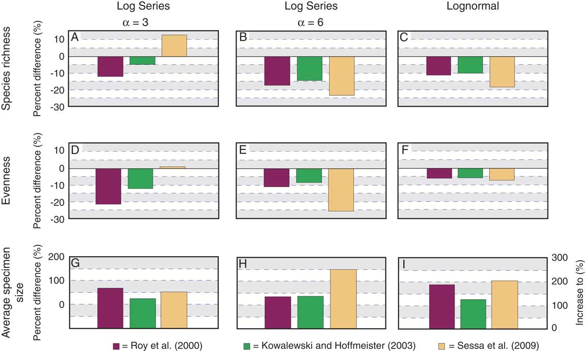
Percentage differences in mean species richness, evenness, and specimen size between the preferential-intersection and random-draw models, produced in nine combinations of three species abundance distributions (log series α=3; log series α=6; lognormal μ=1.2281, σ=1.2408) and three size distributions (Roy et al. Reference Roy, Jablonski and Martien2000; Kowalewski and Hoffmeister Reference Kowalewski and Hoffmeister2003; Sessa et al. Reference Sessa, Patzkowsky and Bralower2009). The differences are displayed as (preferential-intersection value – random-draw value)/random-draw value. For the plot of average specimen size, the vertical axis on the right shows preferential-intersection value/random-draw value (i.e., “increase to” amount rather than “increase by” amount).

Results of model runs (quota=300).

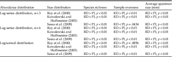
Results of significance tests (quota=300). PI, preferential-intersection model; RD, random-draw model.

Species Richness
The mean richness of samples produced by the preferential-intersection model was consistently less than that produced by the random-draw model using the same combination of species abundance and size distributions (Fig. 8A–C), with the differences ranging from 5% to 23% (Fig. 9A–C). The only exception to this pattern was when the log series with α=3 species abundance distribution was used in conjunction with the Sessa et al. (Reference Sessa, Patzkowsky and Bralower2009) size distribution. When this combination was used, the preferential-intersection model yielded samples that were more species rich, on average, than their counterparts produced by the random-draw model (Figs. 8A and 9A). The offset between the two models was consistently greatest when the Sessa et al. (Reference Sessa, Patzkowsky and Bralower2009) size distribution was used, regardless of which species abundance distribution was used (Figs. 8A–C and 9A–C). The least difference was consistently produced when the Kowalewski and Hoffmeister (Reference Kowalewski and Hoffmeister2003) size distribution was used, again regardless of species abundance distribution (Figs. 8A–C and 9A–C). Comparison of pairs of samples produced using the same species size distribution but different species abundance distributions reveals that the largest percentage difference in species richness is consistently associated with the log-series abundance distribution with α=6 (Fig. 9A–C). Which of the three species abundance distributions produced the least percentage difference between the two models differed depending on which species size distribution was used. When the Kowalewski and Hoffmeister (Reference Kowalewski and Hoffmeister2003) and Sessa et al. (Reference Sessa, Patzkowsky and Bralower2009) size distributions were used, the log-series species abundance distribution with α=3 produced the smallest percentage difference (Fig. 9A). On the other hand, when the Roy et al. (Reference Roy, Jablonski and Martien2000) size distribution was used, the lognormal distribution produced the lowest percentage difference in species richness, slightly less than the value produced using the log series with α=3 (Fig. 9C).
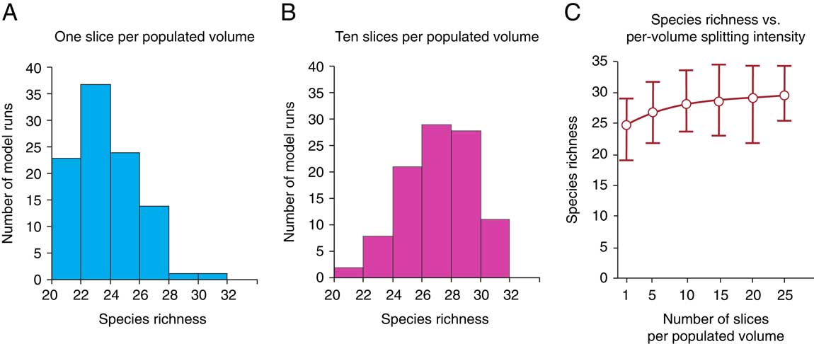
Figure 10 shows how the magnitude of the bias induced by preferential intersection varied as the per volume splitting intensity increased. When each volume was split only once, the preferential-intersection model at a sample size of 100 specimens yielded a mean species richness of 24 species, 6 fewer than the mean of 30 species generated by the random-draw model. This was improved to 26 species when each volume was split 10 times and reached 29 when each volume was split 25 times.
Increase in species richness with per volume splitting intensity, yielded by the preferential-intersection model at a sample size of 100 individuals. Model runs conducted using the Roy et al. (Reference Roy, Jablonski and Martien2000) species size distribution and the lognormal species abundance distribution with μ=1.2281, σ=1.2408, and total species richness=50. A, One splitting plane per populated volume. B, Ten splitting planes per populated volume. C, Increase in species richness with per volume splitting intensity. Brackets represent 95% confidence intervals generated from 150 iterations.

Evenness
The mean evenness of samples produced by the preferential-intersection model was consistently less than that produced by the random-draw model in eight of the nine combinations of species abundance and size distributions (Fig. 8D–F), with the differences ranging from 5% to 25% (Fig. 9D–F). As in the richness analysis, the only exception occurred when the log series with α=3 species abundance distribution was used in conjunction with the Sessa et al. (Reference Sessa, Patzkowsky and Bralower2009) size distribution. However, the combination of species abundance and size distributions that produced the largest and smallest percentage differences in mean evenness between the two models was more variable than for species richness. For each of the three species abundance distributions, different size distributions produced both the largest and smallest percentage difference in evenness between the two models. When the log-series species abundance distribution with α=3 was used, the Roy et al. (Reference Roy, Jablonski and Martien2000) size distribution produced the largest percentage difference between the two models, while the Sessa et al. (Reference Sessa, Patzkowsky and Bralower2009) distribution produced the smallest (Fig. 9D). When the log-series species abundance distribution with α=6 was used, the Sessa et al. (Reference Sessa, Patzkowsky and Bralower2009) size distribution produced the largest difference between the two models, while the Kowalewski and Hoffmeister (Reference Kowalewski and Hoffmeister2003) size distribution produced the smallest one (Fig. 9E). When the lognormal species abundance distribution was used, the Roy et al. (Reference Roy, Jablonski and Martien2000) and Kowalewski and Hoffmeister (Reference Kowalewski and Hoffmeister2003) size distributions produced a similar percentage difference, which is smaller than that produced by the Sessa et al. (Reference Sessa, Patzkowsky and Bralower2009) size distribution (Fig. 9F).
When comparing model runs using the Roy et al. (Reference Roy, Jablonski and Martien2000) size distribution but different species abundance distributions, the log-series species abundance distribution with α=3 produced the largest and the lognormal species abundance distribution produced the smallest percentage differences between the two models (Fig. 9D–F). The same is true for the Kowalewski and Hoffmeister (Reference Kowalewski and Hoffmeister2003) size distribution. By contrast, when the Sessa et al. (Reference Sessa, Patzkowsky and Bralower2009) size distribution was used, the log-series distribution with α=3 produced the smallest difference between the two models (Fig. 9D), whereas the log series with α=6 produced the largest difference (Fig. 9E).
Average Specimen Size
The mean values of the average size of specimens produced by the preferential-intersection model were consistently greater than those produced by the random-draw model. The Kowalewski and Hoffmeister (Reference Kowalewski and Hoffmeister2003) size distribution consistently produced the smallest percentage difference between the two models, regardless of which species abundance distribution was used (Fig. 9G–I). For both the log-series species abundance distribution with α=6 and the lognormal distribution, the Sessa et al. (Reference Sessa, Patzkowsky and Bralower2009) size distribution produced the largest percentage difference in average specimen size between the two models (Fig. 9H–I). For the log-series species abundance distribution with α=3, the Roy et al. (Reference Roy, Jablonski and Martien2000) size distribution produced the largest percentage difference (Fig. 9G).
t-Test Results
Table 2 shows the results of two-tailed t-tests conducted on sets of species richness, evenness, and average specimen size values produced by the preferential-intersection and random-draw models for each combination of species abundance and size distributions at a sampling quota of 300 specimens. All but one of the tests yielded a p-value below 0.05. The only test that yielded a p-value greater than 0.05 was for values of evenness produced using the Roy et al. (Reference Roy, Jablonski and Martien2000) size distribution and the lognormal species abundance distribution.
Discussion
Preferential Intersection as a Component of the Lithification Bias on Species Richness
The model results presented above demonstrate that fossil sampling from well-lithified sediments via splitting rock can bias aspects of species diversity even without the loss of specimens due to aragonite dissolution, mechanical breakage, or the Chlamys effect. Determining the extent to which preferential intersection can explain the observed lithification bias, either in part or in whole, requires comparing the model results with empirical studies. The largest percentage difference in species richness between the random-draw and preferential-intersection models was consistently generated when the log-series species abundance distribution was used with α=6 (Fig. 9C). Random-draw models with this species abundance distribution produced average species richness of 22–23 at a sample intensity of n=100 (Fig. 6A–C), which is close to the average species richness of 20 reported by Hendy (Reference Hendy2009) for samples of size n=100 from unlithified sediments. Hendy (Reference Hendy2009) found that lithified samples yielded collections that were 50% less species rich than unlithified samples, with average species richness values around 10 species. Sessa et al. (Reference Sessa, Patzkowsky and Bralower2009) also reported an average species richness of 20 for unlithified sediments at a sample size of 100 individuals. Sessa et al. (Reference Sessa, Patzkowsky and Bralower2009) reported an even greater difference between lithified and unlithified collections, with their lithified collections yielding an average richness of only five species, a decrease in species richness of 75%. Given that, for the log series with α=6, our model produced average decreases in species richness of 14–23% (Fig. 9B), preferential intersection can account for 18–45% of the empirically observed bias reported in the literature. Because these represent the maximum decreases in species richness among the three chosen species abundance distributions, they are considered the “worst-case scenarios.”
Because preferential intersection cannot explain the entire observed richness difference between lithified and unlithified sediments, other mechanisms must be invoked to explain the remaining difference in diversity. The most obvious candidates are the two additional mechanisms for the lithification bias that have been proposed in the literature—namely, dissolution of small aragonitic specimens (Hendy Reference Hendy2009) and mechanical destruction during splitting (Kowalewski et al. Reference Kowalewski, Wood, Kiessling, Aberhan, Fürsich, Scarponi and Hoffmeister2006). Additional factors may also contribute to the lithification bias, including the Chlamys effect (Kowalewski et al. Reference Kowalewski, Carroll, Casazza, Gupta, Hannisdal, Hendy, Richard, LaBarbera, Lazo and Messina2003), that is, fragments of some species are more easily identifiable than those of others, particularly when samples are processed in the laboratory and microscopes are used. All three of these mechanisms have the potential to bias against small-sized taxa. The small, thin-shelled aragonitic taxa that are at the highest risk for dissolution are also the most likely to be missed due to preferential intersection, and they are also the most vulnerable to mechanical breakage during collection. The Chlamys effect could potentially bias against small specimens if the preservation of diagnostic features is itself size dependent. For example, small specimens preserved as steinkerns in sandstone may not exhibit sufficient detail to be identifiable, whereas larger specimens may. It follows from these considerations that the effects of these biases are more likely to be redundant than additive. An assemblage that has lost its smallest taxa due to aragonite dissolution is likely to yield similar diversity values whether collected via sieving sediments or splitting rock, because those specimens that were most vulnerable to the effects of preferential intersection have already been removed. At the same time, fossil assemblages may exhibit similar losses of small taxa due to any combination of the above mechanisms. Demonstrating that a fossil assemblage has not been significantly affected by one of these mechanisms does not imply that it is unaffected by the others. For example, demonstrating the presence of abundant aragonitic taxa within lithified assemblages does not necessarily mean that preferential intersection does not exert a bias.
Establishing the degree to which these mechanisms actually contribute to the observed lithification bias and how their relative importance varies from case to case requires further work. Nevertheless, both taphonomic and sampling processes can bias species richness, evenness, or average specimen size, raising an important point about conceptual clarity. The term “lithification bias” is arguably somewhat misleading, because it incorrectly implies that biasing effects occurred during the diagenetic transition of unconsolidated sediments to fully indurated rock. However, as originally defined by Hendy (Reference Hendy2009) and Sessa et al. (Reference Sessa, Patzkowsky and Bralower2009), the term “lithification bias” simply refers to the fact that fossil assemblages from lithified sediments frequently exhibit lower diversity than their counterparts from unconsolidated sediments even after being corrected for differences in sample size. As argued here and elsewhere (Nawrot Reference Nawrot2012), this empirical difference can in principle result from processes that occurred at any point between lithification and fossil collection, including both taphonomic and sampling processes. Any discussion of the lithification bias should therefore clearly distinguish between the bias itself and its potential contributing mechanisms.
Comparison with Other Studies of the Lithification Bias
Several other authors have previously attempted to disentangle the factors that contribute to the lithification bias, and a comparison of their results with ours reveals some important similarities. Daley and Bush (Reference Daley and Bush2012, Reference Daley and Bush2014) created artificial fossiliferous rocks using Portland cement and compared them with identical fossil assemblages from unconsolidated sediments. Daley and Bush (Reference Daley and Bush2014) found that, while in some cases their artificial rocks yielded samples with lower diversity than samples from unconsolidated sediments, in other instances their artificial rocks actually yielded more diverse samples. As noted earlier, the occurrence of higher diversity in samples collected via preferential intersection was also observed in one of our model runs (Figs. 8A and 9A). Instances of enhanced diversity in samples collected via preferential intersection can be explained by rare species with larger sizes, which have a relatively greater chance of intersection and thus sampling. This effect offers a possible explanation for the enhanced diversity related to lithification state observed by Daley and Bush (Reference Daley and Bush2014). This highlights the crucial fact that species size and abundance distributions affect how preferential-intersection biases sample diversity. If a greater number of less-abundant species have sizes that fall on the smaller end of the size spectrum, then sampling via preferential intersection will tend to generate less-diverse samples, whereas the opposite will occur if rare taxa fall on the larger end. Daley and Bush (Reference Daley and Bush2014) proposed an alternative mechanism to explain the higher diversity they observed in lithified samples: careful and nonrandom scanning of lithified surfaces may reveal previously unsampled species and thus greater diversity than unlithified samples. Our model does not address this worker-generated bias; however, it remains a potential contributing factor.
Nawrot (Reference Nawrot2012) attempted to separate out sampling methodology and diagenetic effects as contributing factors to the lithification bias by examining molluscan faunas within storm-beach rock. This analysis was based on the assumption that, since the storm-beach rock was cemented during earliest diagenesis, little dissolution of aragonitic components of the fauna had occurred. In contrast to other studies of the lithification bias, Nawrot (Reference Nawrot2012) found little to no significant difference in species richness between lithified and unlithified sediments, although he did find significant differences in the relative abundances of taxa. Nawrot (Reference Nawrot2012) inferred that loss of specimens during diagenesis was the dominant driver of the decline in species richness. Comparison of the results of Nawrot (Reference Nawrot2012) with those produced by the model suggests that, in spite of the fact that the model makes simplified assumptions, it can faithfully reproduce results seen in empirical studies of the lithification bias in cases in which the effects of specimen loss due to dissolution are negligible. Given that the fossil assemblages studied by Nawrot (Reference Nawrot2012) were low-evenness assemblages dominated by small taxa, they most closely resemble the model runs that used α=3 and the Kowalewski and Hoffmeister (Reference Kowalewski and Hoffmeister2003) size distribution. Although the lithology of the fossil samples studied by Nawrot (Reference Nawrot2012) most closely matches the “partially lithified” category of Hendy (Reference Hendy2009), which was less susceptible to bias than fully lithified sediments, Nawrot’s (Reference Nawrot2012) collection procedure consisted of splitting rock and counting specimens on the exposed surface. The exposed specimens were then extracted from the matrix for taxonomic identification to ensure complete sampling and identification (R. Nawrot, personal communication). This sampling procedure is akin to our preferential-intersection model, which counts and identifies every exposed specimen, whereas this is not true in many other empirical studies. Thus, it is most appropriate to compare our model results with Nawrot’s (Reference Nawrot2012) empirical results, because Nawrot (Reference Nawrot2012) also avoided some of the same complicating factors (e.g., dissolution of aragonitic shells) that our model does not take into account. At n=100, Nawrot (Reference Nawrot2012) observed an average species richness difference between lithified and unlithified sediments of only one species, equivalent to 5% of the total diversity. This is similar to the modeling results obtained using α=3 and the Kowalewski and Hoffmeister (Reference Kowalewski and Hoffmeister2003) size distribution, which yielded a species richness difference of 1.4 species at n=100. Thus, bias estimates produced in theoretical modeling presented here are remarkably consistent with empirical estimates reported previously.
The work of both Daley and Bush (Reference Daley and Bush2014) and Nawrot (Reference Nawrot2012) represent thoughtful ways of attacking the problem of distinguishing factors that contribute to the lithification bias using actual fossil samples as opposed to the in silico approach used here. Integrating the different approaches is likely to yield further insights. Bulk samples collected in box cores, which would allow careful halving analogous to a flat-fracture plane, represent an additional potential approach for looking at how sampling on exposed surfaces compares with collecting all specimens in a volume.
Impact of Preferential Intersection on Older Fossil Assemblages
The analyses of preferential intersection performed here were based on size and aspect ratio data derived from assemblages of Cenozoic mollusks (Roy et al. Reference Roy, Jablonski and Martien2000; Kowalewski and Hoffmeister Reference Kowalewski and Hoffmeister2003; Sessa et al. Reference Sessa, Patzkowsky and Bralower2009). The impact of preferential intersection on diversity measures of brachiopod-dominated Paleozoic assemblages and brachiopod–mollusk Mesozoic assemblages must await further studies, since the ranges of size and shape used here may not be applicable to these older assemblages. At this point we can only offer educated speculation on the likely impact of preferential intersection on Paleozoic and early Mesozoic assemblages, with the caveat that further modeling work targeting these assemblages is needed.
The Paleozoic fossil record is derived almost exclusively from well-lithified sedimentary rocks (Hendy Reference Hendy2009), and examinations of evenness through the Phanerozoic suggest that Paleozoic assemblages are predominantly low-evenness, high-dominance assemblages (Powell and Kowalewski Reference Powell and Kowalewski2002; Bush and Bambach Reference Bush and Bambach2015). Wagner et al. (Reference Wagner, Kosnik and Lidgard2006) also found that Paleozoic assemblages are best described by the log-series species abundance distribution. Thus, they most closely resemble samples in this study fitting the log-series distribution with α=3. For these low-diversity assemblages, this translates to absolute differences of only one or two species. However, it is possible that this low-diversity character is itself the result of the lithification megabias. While the modeling results presented here do not address all mechanisms that potentially contribute to the lithification megabias, they do help us to better understand the degree to which preferential intersection may have affected the diversity of Paleozoic assemblages. To distinguish whether Paleozoic assemblages are intrinsically low in diversity or were strongly affected by the preferential-intersection bias because they exclusively come from lithified rocks, we can evaluate whether any of the model results presented here show a reduction of species richness and evenness to levels seen in Paleozoic samples. If any preferential-intersection model runs yielded species richness or evenness values comparable to those seen in Paleozoic samples, then it is possible that the true species richness and evenness would be closer to what is produced by the random-draw model with the same parent distribution. Modeling results using a log-series distribution with α=3 produced richness values of 11–12 species at n=100 specimens, comparable to Paleozoic samples. However, in this parameterization, the difference in species richness between preferential intersection and random draw is only one to two species, indicating that preferential intersection only had a limited effect. When the log series with α=6 or the lognormal distribution was used, a greater reduction in species richness was seen, but the species richness produced by the preferential-intersection model did not match the low values of Paleozoic samples. It is possible that, under other unexplored parameterizations, preferential intersection could generate a greater decrease in richness and evenness relative to the random-draw model and reach the low levels seen in Paleozoic samples. However, further considerations discussed below reinforce the idea that the diversity estimates of Paleozoic assemblages are unlikely to have been significantly skewed by preferential intersection.
Paleozoic fossil assemblages are frequently collected from fossil concentrations such as shell beds, pavements, and lags, in contrast to our models, in which fossils are randomly distributed in the rock volume. Paleozoic shells beds are typically <20 cm and often just a few centimeters in thickness, much thinner than their Cenozoic counterparts (Kidwell and Brenchley Reference Kidwell and Brenchley1994). In a study of Ordovician shell beds in the Basin and Range Province, Li and Droser (Reference Li and Droser1999) consistently found that the majority of shell beds are <10 cm in thickness. In comparison, the cubic volumes generated by our models have a vertical height of 10 cm, corresponding to the larger end of Paleozoic shell-bed thickness. Intuitively, the thinner the shell bed, the less opportunity for preferential intersection to exert a significant effect. When excavated, extremely thin shell beds would expose all or nearly all specimens, and no preferential-intersection bias would be expected. In slightly thicker shell beds, fractures are guided by larger specimens in the fossil concentrations. Thus, fractures would “find” larger specimens and also expose nearby smaller specimens, given the proximity of specimens. Considering that many Paleozoic assemblages come from relatively thin fossil concentrations, the preferential-intersection bias is likely mitigated to a certain degree.
Fossil concentrations not only guide fractures, but also direct collection efforts. Exhaustive efforts to break up samples, to expose even the smallest specimens, and to sample the rarest taxa in shell beds would overcome the preferential-intersection bias to some degree. Unfortunately, methodological details given in the literature are often not explicit about the degree to which bulk samples were broken up. Also, thin Paleozoic shell beds are often covered by shale or mudstone that either weathers readily or else can be easily mechanically removed, revealing well-preserved specimens.
Taking all of the above into account, it is likely that the biasing effect of preferential intersection on species richness of brachiopod-dominated Paleozoic assemblages would be no greater than the lowest differences observed in this study. However, even if the impact of preferential intersection on brachiopod-dominated Paleozoic assemblages were determined to be negligible, it would not necessarily follow that species richness of these assemblages are unaffected by other biasing mechanisms, only that preferential intersection can be ignored for these cases, and that any instance of lithification-related bias affecting species richness in brachiopod-dominated Paleozoic assemblages must be driven by other mechanisms.
As an encouraging note, our modeling to investigate the impact of per volume splitting intensity shows that, at least for some combinations of species size and abundance distributions, the preferential intersection can potentially be overcome through a deliberate splitting strategy. As splitting intensity increases and splitting planes are more closely placed, small specimens are more likely to be intersected by at least one splitting plane (Fig. 10; Supplementary Appendix II). In other words, sufficiently exhaustive sample preparation can overcome the effects of preferential intersection.
Conclusion
Understanding how to correct for lithification biases requires identifying the process or processes that generate such biases. The work presented here demonstrates that preferential intersection (i.e., the higher probability of sampling larger specimens relative to smaller ones due to their greater likelihood of being intersected and thus being visible on split surfaces) can have a biasing effect on species richness, sample evenness, and average specimen size of fossil samples. Average specimen size in particular can be significantly skewed by the effects of preferential intersection, a finding with potentially important implications for studies of the evolution of body size through the Phanerozoic. Preferential intersection is therefore a potential contributing factor to the lithification bias, and the magnitude of this bias is partially dependent on species abundance and size distributions. Our study also suggests that preferential intersection cannot fully explain observed differences between lithified and unlithified fossil assemblages, and therefore other mechanisms such as aragonite dissolution, mechanical breakage, and possibly other factors such as the Chlamys effect likely also contribute to the lithification bias. Nevertheless, the biasing effect of preferential intersection should be taken into account when fossil collections are made by splitting well-lithified sedimentary rocks, particularly those with sparse fossil contents. This work demonstrates that the empirically observed lithification bias is complex and, at least in some cases, may be the result of multiple factors and should not be considered synonymous with the aragonite bias.
Acknowledgments
This work was supported by NASA Exobiology and Evolutionary Biology Program (NNX15AL27G), NSF Sedimentary Geology and Paleobiology Program (EAR-1528553), Paleontological Society, and Virginia Tech Department of Geosciences. Brian Romans and Benjamin Gill provided helpful comments and suggestions at various stages throughout the project. Kaustuv Roy, Rafał Nawrot, and an anonymous reviewer provided constructive comments on this paper.
Supplementary material
Data available from the Dryad Digital Repository: http://dx.doi.org/10.5061/dryad.p85q4