Introduction
The dominance of invasive aquatic plant species can lead to numerous negative impacts on aquatic ecosystems. Through competition and displacement, invasive aquatic plants reduce native plant diversity and ultimately form dense monotypic stands of vegetation (Gause Reference Gause1934; Hardin Reference Hardin1960; Schultz and Dibble Reference Schultz and Dibble2012). These dense monotypic stands can reduce native fish and macroinvertebrate populations and diversity (Covich et al. Reference Covich, Austen, Bärlocher, Chauvet, Cardinale, Biles, Inchausti, Dangles, Solan, Gessner, Statzner and Moss2004; Downing and Leibold Reference Downing and Leibold2002). They can also reduce overall ecosystem productivity and impede the natural flow of water through an ecosystem (Engelhardt and Ritchie Reference Engelhardt and Ritchie2002; Pitlo and Dawson Reference Pitlo, Dawson, Pieterse and Murphy1993; Schultz and Dibble Reference Schultz and Dibble2012). Additionally, these infestations negatively impact the recreational utility of bodies of water, reduce property values, and create habitat suitable for disease-carrying vectors (Gangstad and Cardarelli Reference Gangstad, Cardarelli, Pieterse and Murphy1993; Halstead et al. Reference Halstead, Michaud and Hallas-Burt2003; Wilde et al. Reference Wilde, Murphy, Hope, Habrun, Kempton, Birrenkott, Wiley, Bowerman and Lewitus2005; Zhang and Boyle Reference Zhang and Boyle2010).
Herbicides are one of the most commonly used and cost-effective methodologies for the selective management of invasive aquatic weeds. Currently, there is a need for additional active ingredients in aquatic systems to respond to new threats or treatment scenarios, enhance selectivity, reduce use rates, and mitigate the risk of herbicide resistance (Cobb and Reade Reference Cobb and Reade2010; Getsinger et al. Reference Getsinger, Netherland, Grue and Koschnick2008).
Synthetic auxin herbicides have favorable properties for invasive plant control as they (1) pose limited risk to wildlife; (2) are easily absorbed and translocated throughout sensitive plants; and (3) are generally selective to control dicots, with minimal impact to monocots (Epp et al. Reference Epp, Alexander, Balko, Buysse, Brewster, Bryan, Daeuble, Fields, Gast, Green, Irvine, Lo, Lowe, Rnega and Richburg2016; Grossmann Reference Grossmann2010; Netherland Reference Netherland, Gettys, Haller and Bellaud2009). Only 17 herbicides and algaecides are currently registered for aquatic use, two of which, triclopyr and 2,4-D, can be considered auxin mimics (Netherland Reference Netherland, Gettys, Haller and Bellaud2009). Recently, a new herbicide, florpyrauxifen-benzyl, was developed and registered for use in aquatics. Florpyrauxifen-benzyl is a synthetic auxin with a highly favorable toxicology profile (Miller and Norsworthy Reference Miller and Norsworthy2015; Wells and Taylor Reference Wells and Taylor2016). This herbicide has been shown to be highly effective in controlling some of the most invasive aquatic plant species in the United States, including hydrilla [Hydrilla verticillata (L. f.) Royle] and invasive watermilfoils (Myriophyllum spp.) (Netherland and Richardson Reference Netherland and Richardson2016; Richardson et al. Reference Richardson, Haug and Netherland2016).
To better understand the interaction between in-water herbicide concentrations and target species, it is important to understand herbicide absorption and translocation kinetics. Theoretically, the carboxylic acid functional group on florpyrauxifen-benzyl (lipid soluble) and other picolinate auxin herbicides allows for the herbicide to pass through the lipophilic phloem wall, and with a low pKa, the herbicide should ionize into the anionic form inside the phloem, effectively concentrating the herbicide in the phloem (Bromilow et al. Reference Bromilow, Chamerlain and Evans1990; Epp et al. Reference Epp, Alexander, Balko, Buysse, Brewster, Bryan, Daeuble, Fields, Gast, Green, Irvine, Lo, Lowe, Rnega and Richburg2016). This process is called “phloem trapping” and would allow for systemic movement of the ionized herbicide to growing shoot and root tissues (Epp et al. Reference Epp, Alexander, Balko, Buysse, Brewster, Bryan, Daeuble, Fields, Gast, Green, Irvine, Lo, Lowe, Rnega and Richburg2016). However, plant response to synthetic auxins is often species specific and may vary in an aquatic environment compared with a terrestrial environment (Cobb and Reade Reference Cobb and Reade2010; Delbarre et al. Reference Delbarre, Muller, Imhoff and Guern1996). Therefore, absorption and translocation of florpyrauxifen-benzyl need to be evaluated for species-specific responses to confirm theoretical hypotheses regarding the behavior of this herbicide within aquatic plants. In the last several years, protocols employing radiolabeled herbicides have been used to study the absorption and translocation of some herbicides in aquatic plants (Kniss et al. Reference Kniss, Vassios, Nissen and Ritz2011; True-Meadows 2012; Vassios et al. Reference Vassios, Nissen, Koschnick and Heilman2014, Reference Vassios, Nissen, Koschnick and Heilman2017). The objective of this study was to elucidate absorption and translocation kinetics of florpyrauxifen-benzyl in 10 important aquatic plant species.
Materials and Methods
The methodology utilized in this study closely follows that of Vassios et al. (Reference Vassios, Nissen, Koschnick and Heilman2014). Adaptations and specifics are discussed in the following sections.
Plant Propagation and Preparation
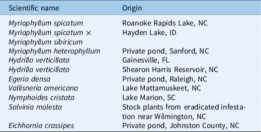
The 10 aquatic plant species utilized in this experiment were Eurasian watermilfoil (Myriophyllum spicatum L.), hybrid Eurasian watermilfoil (Myriophyllum spicatum L. × Myriophyllum sibiricum Kom.), variable watermilfoil (Myriophyllum heterophyllum Michx.), dioecious hydrilla, monoecious hydrilla, Brazilian egeria (Egeria densa Planch.), American eelgrass (Vallisneria americana Michx.), crested floatingheart [Nymphoides cristata (Roxb.) Kuntze], giant salvinia (Salvinia molesta Mitchell), and waterhyacinth [Eichhornia crassipes (Mart.) Solms]. Plant source locations are listed in Table 1. Submersed species and N. cristata were planted in flat-bottom 25-mm-diameter glass test tubes. The test tubes were filled with sterilized topsoil amended with slow-release fertilizer (Osmocote Smart Release 15-9-12®, Scotts, 14111 Scottslawn Road, Marysville, OH 43041) at a rate of 3 g L−1 of soil. Fifteen-centimeter apical segments were cut from stock plants and planted in the fertilizer-amended topsoil, and a thin layer of sand was placed on top. Once planted, submersed plants were established in dechlorinated tap water in a glass greenhouse with 30% shade cloth for 8 wk, with the exception of hybrid M. spicatum × M. sibiricum. Due to poor growth following initial planting, new 15-cm apical segments of hybrid M. spicatum × M. sibiricum were planted 2 wk before treatment. At the same time, submersed species that had been growing for 6 wk were trimmed to approximately 15 cm of shoot tissue. At 1 wk before treatment, plants were moved to the treatment room to acclimate. Treatment vessels were maintained under full-spectrum lights (21 µmol s−1 m−2) with a 14-h light:10-h dark light regime for the duration of the experiment. Natural sunlight was blocked from entering the room just before and throughout the treatment. Air temperature was maintained at 23 ± 3 C, and air was circulated constantly throughout the experiment.
A list of the plant species used in this experiment and the origins of the plant collections.

One to two days before treatment, plants were briefly removed from the growth chambers and placed in test tube racks with the majority of shoot tissue submerged in adjacent beakers of dechlorinated tap water. Water was dried from the surface of the sand and the walls of the test tube using paper towels to provide a tighter seal between the gel and the wall of the test tube. Once the surfaces were dried, a layer of agarose gel (1.5% v/v) (Phytagar, Invitrogen, Grand Island, NY 14075) was placed on the sand surface. The gel was maintained in a liquid state at a temperature of 30 to 38 C.
Two floating species, S. molesta, and E. crassipes, were also included in this experiment. Small (5- to 7-cm diameter) daughter plants of E. crassipes and small (3- to 5-node) S. molesta plants were selected from established stock plants. Because roots were already established on these plants, they were immediately transferred to the treatment room to acclimate without an establishment period. No agar separation was applied to floating species.
Shoot Absorption and Translocation
Treatments were carried out in a temperature- and light-controlled room. Glass treatment vessels (7.6 L) were filled with 7 L of tap water treated with water conditioner (API Tap Water Conditioner®, Mars Fishcare North America, 50 E. Hamilton Street, Chalfont, PA 18914). Each treatment vessel was equipped with a custom-built, 24-slot, stainless-steel test tube rack. To contain the 10 species slated for treatment, two tank types labeled “Tank A” and Tank B” were established, each with 4 submersed species and 1 floating species. Each tank type was replicated three times for a total of six treatment tanks. Six experimental units of five species were placed in Tank A and in Tank B for a total of 30 plants per tank. Ten different species were represented across the two tank types. Tank A species were N. cristata, dioecious H. verticillata, M. spicatum, S. molesta, and M. heterophyllum. Tank B species were E. densa, hybrid M. spicatum × M. sibiricum, monoecious H. verticillata, V. americana, and E. crassipes. Plants were placed in test tube racks within holding buckets before treatment, and all plants were lowered into the treatment vessels following application of the 14C-labeled herbicide and formulation blank.
All six treatment vessels were treated at a rate of 10 µg ai L−1 florpyrauxifen-benzyl. A mixture of 75% nonradiolabeled technical material, 25% radiolabeled technical material, and sufficient formulation blank equivalent to the 300 g ai L−1 suspension concentrate commercial aquatic formulation (Procellacor SC, Dow AgroSciences, Specialty Synthesis Group, Indianapolis, IN 46268) was used to reach this target treatment rate. Radiolabeled and nonradiolabeled technical materials were dissolved in acetone separately. The radioactivity of the labeled solution was confirmed using a liquid scintillation counter (LSC), the concentration of the nonlabeled solution was confirmed via HPLC-MS, and then the two solutions were mixed with ratio of 25 labeled:75 nonlabeled. The formulation blank was diluted in water before application. Dissolved technical material was applied to the treatment vessels, followed immediately by the application of diluted formulation blank. The vessel was then stirred with a glass stirring rod to ensure uniform distribution of active ingredients and formulation. Following application, the test tube racks containing the plants to be treated were placed in each of the treatment vessels. This placement marked time zero for treatment, and three replicate plants of each species were harvested without exposure to treatment vessels.
Plants were harvested at 0, 0.5, 1, 6, 12, 36, and 192 h following treatment. Preliminary studies had shown that florpyrauxifen-benzyl is absorbed very quickly (EJH, unpublished data, 2017). As such, these harvest times were selected to be more heavily weighted toward earlier times after treatment, compared with other studies, to capture the initial hyperbolic increase in absorption. At each designated harvest time, three replicate plants of each species were removed from the treatment vessels. Above- and belowground material was removed from the test tube and separated at the agar line. Each tissue type was triple rinsed with distilled water separately and then allowed to air dry. One milliliter of rinsate from the third rinse of each plant portion was analyzed by LSC to ensure that all surface radiation was removed and only absorbed radiolabeled material remained. Following 1 to 2 h of air-drying, plant tissue was placed in a paper bag. Paper bags with plant tissue were dried at 70 C for 48 h. Dry biomass data were collected for each plant tissue type using an analytical balance. Plant tissue was then rolled in ash-free filter paper, labeled, and stored at −4 C. Plant tissue and filter paper were combusted in a biological oxidizer (OX500®, RJ Harvey Instrument, 11 Jane Street, Tappan, NY 10983) for 2 min and collected in 15 ml of 14C-trapping oxidizing cocktail (OX161®, RJ Harvey Instrument). The efficiency of the oxidizer was confirmed daily to meet EPA standards of 80% to 120% recovery. Following combustion, the radioactivity of samples was quantified by LSC (Tri-carb 2100TR Liquid Scintillation Counter®, Spectrofuge Corporation of North Carolina, 4915 Prospectus Drive, Suite A, Durham, NC 27713) for 4 min per sample. The trial was replicated twice separated in time.
Statistical Analysis
The statistical analyses followed those of Vassios et al. (Reference Vassios, Nissen, Koschnick and Heilman2014, Reference Vassios, Nissen, Koschnick and Heilman2017). Herbicide concentration in micrograms of herbicide per gram of dry weight was calculated in Microsoft Excel (2010, Microsoft, Redmond, WA 98052) utilizing measured disintegrations per minute (dpm) of each sample, the measured dry biomass of each sample analyzed, and the specific activity of the radiolabeled florpyrauxifen-benzyl received. Levene’s test for homogeneity of variance was run in MS Excel for each species before combining the two runs of concentration data for analysis. Following the Levene’s test, means and standard errors were calculated using the JMP Pro (v. 13, SAS Institute, Cary, NC 27513) extension platform for SAS software. These tabulated values were then exported back to MS Excel and finally imported into SigmaPlot (v. 13, Systat Software, San Jose, CA 95110) for nonlinear regression analysis. The regression analysis fit the hyperbolic model adapted from Kniss et al. (Reference Kniss, Vassios, Nissen and Ritz2011) by Vassios et al. (Reference Vassios, Nissen, Koschnick and Heilman2014, Reference Vassios, Nissen, Koschnick and Heilman2017) (Equation 1), where y is the predicted absorption at time x, and a and b are constants. Regression equations for belowground tissue for monoecious H. verticillata, dioecious H. verticillata, and hybrid M. spicatum × M. sibiricum could not be calculated in SigmaPlot using the nonhyperbolic regression equation (Equation 1) and were therefore excluded from the results.
 $$y = {{ax} \over {1 + bx}}$$
The plant concentration factor (PCF) metric is often used to compare absorption across different herbicides with varying properties and applied at varying rates. While this experiment focused on the absorption and translocation of only one herbicide at one rate, we felt the inclusion of the PCF metric would be beneficial for future comparisons across studies. PCF was calculated following the equation presented in Vassios et al. (Reference Vassios, Nissen, Koschnick and Heilman2017) as adapted from de Carvalho et al. (Reference De Carvalho, Bomilow and Greenwood2007) (Equation 2), where plant concentration is the concentration of the herbicide (ng) in plant tissues divided by the fresh biomass (g), and water concentration is the concentration of the herbicide in the treated water at the time of treatment (ng ml−1).
 $${\rm{PCF}} = {{{\rm{plant}}\,{\rm{concentration}}} \over {{\rm{water}}\,{\rm{concentration}}\;}}$$
The nonlinear regression equations resulting from these analyses were used to calculate the predicted absorption at 192 h after treatment (HAT) (A192) and the predicted time it would take to reach 90% of that absorption (t 90). These two metrics were recommended for comparisons of absorption in different species and plant portions in Vassios et al. (Reference Vassios, Nissen, Koschnick and Heilman2017). The A192 value was used to compare the theoretical maximum absorption of different species, and t 90 was used to compare the rate of absorption or how quickly the plant absorbed to its maximum.
It is important to note that fresh weights were only collected during run 2. Linear regression equations of second-run dry weight to fresh weight comparisons were conducted for each species with separate equations for shoot (r2 = 0.48 to 0.97; P < 0.001) and root tissue (r2 = 0.49 to 0.95; P < 0.001). The equations were used to estimate the fresh weights for run 1 samples.
Translocation of herbicide from aboveground to belowground tissue was calculated as the percent of total radioactivity in the plant that was observed in the belowground portion of the plant. The mean and standard error of this value for each time interval (hours after treatment) were plotted using JMP Pro (v. 13) graph builder.
Results and Discussion
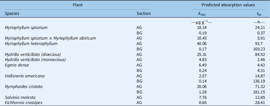
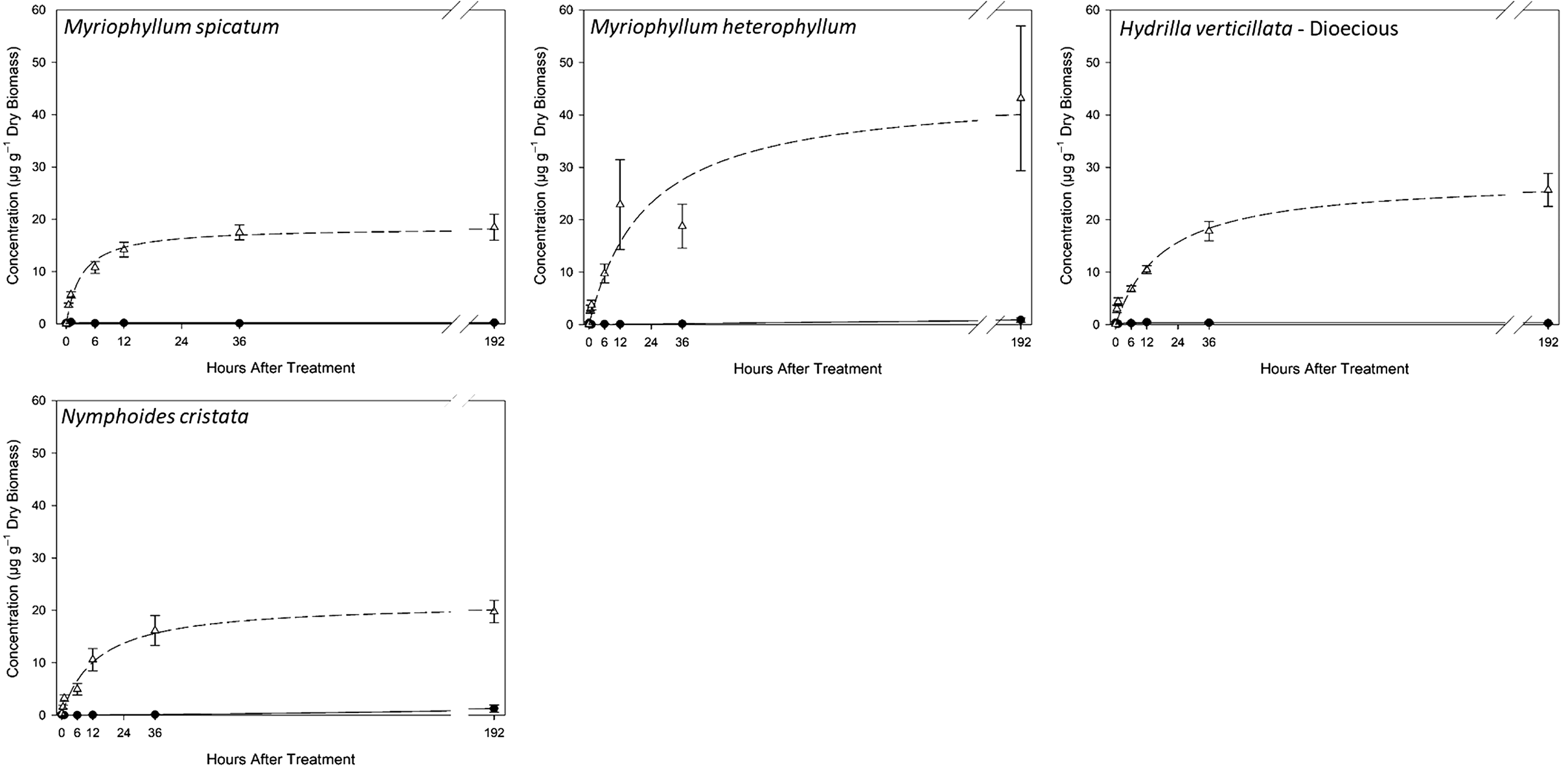
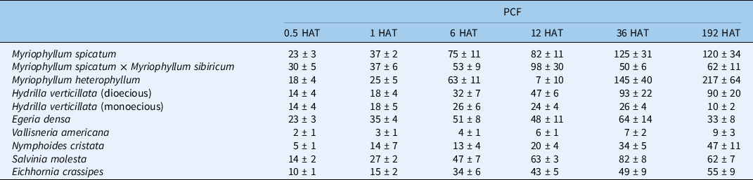
The hyperbolic regression model fit M. spicatum aboveground florpyrauxifen-benzyl accumulation over time (r2 = 0.98; Table 2; Figure 1). A rapid increase in product concentration in the plant was observed within the first 24 h, and this is reflected by the predicted t 90 value of 24.21 h (Table 2). Results from PCF also show this maximum concentration occurring between the 12- and 36-h harvests (Table 3). The PCF192 (120) and A192 (18.14 µg g−1) indicate very high levels of absorption for M. spicatum (Tables 2 and 3). The M. spicatum PCF192 (120 ± 34) for florpyrauxifen-benzyl was more than twice the M. spicatum PCF192 (35 ± 6) reported for triclopyr, another synthetic auxin (Vassios et al. Reference Vassios, Nissen, Koschnick and Heilman2017). This discrepancy indicates that florpyrauxifen-benzyl bioconcentrates in M. spicatum tissues to a greater extent than triclopyr. The results were not unexpected, given the high level of sensitivity of M. spicatum to florpyrauxifen-benzyl observed in other studies (Netherland and Richardson Reference Netherland and Richardson2016).
Results of hyperbolic regression analysis and predicted values for the absorption (µg g−1) at 192 h (A192) and the time in hours to reach 90% of A192 (t 90) for aboveground (AG) and belowground (BG) tissue.

Hyperbolic nonlinear regression plots for Myriophyllum spicatum, Myriophyllum heterophyllum, dioecious Hydrilla verticillata, and Nymphoides cristata. Aboveground data are symbolized with a dashed line for the regression and open triangles for the mean concentration. Belowground data are symbolized with a solid line for the regression and closed circles for the mean concentration. Error bars represent the standard error of the mean. Please note the y axis scales in this figure display a maximum concentration of 60 µg g−1 dry biomass compared with only 20 µg g−1 dry biomass in Figure 2.

Plant concentration factor (PCF) results for each species at each time interval in hours after treatment (HAT) expressed as the mean ± standard error.

Results of belowground tissue analysis indicate only limited translocation to root tissue with an A192 of 0.19 µg g−1 (Table 2), and an average translocation of 0.48 ± 0.28% at 192 HAT (data not shown). Vassios et al. (Reference Vassios, Nissen, Koschnick and Heilman2014) found a high accumulation of triclopyr, an auxin-mimic herbicide, with both granular and liquid formulations; however, the authors indicate this may have been due in part to movement within the soil pore water, as the shoots and roots were not separated. In another study, Vassios et al. (Reference Vassios, Nissen, Koschnick and Heilman2017) observed only 2.6 ± 0.3% of the absorbed triclopyr herbicide was translocated to belowground tissue. The high herbicidal activity of florpyrauxifen-benzyl compared with triclopyr may be relevant in interpreting translocation. Small-scale screening has documented that florpyrauxifen-benzyl is as much as 370 times more active on M. spicatum than triclopyr (Beets and Netherland Reference Beets and Netherland2018). Vassios et al. (Reference Vassios, Nissen, Koschnick and Heilman2017) observed a belowground A192 of 71.42 µg ai g−1 with triclopyr in M. spicatum.
Absorption values for hybrid M. spicatum × M. sibiricum (A192 = 10.43 µg g−1; PCF192 = 62 ± 11) were lower than that of M. spicatum (A192 = 18.14 µg g−1; PCF192 = 120 ± 34) (Tables 2 and 3). However, hybrid M. spicatum × M. sibiricum reached 90% of maximum absorption faster (t 90 = 5.91 h) than M. spicatum (t 90 = 24.21 h) (Table 2). The lower absorption and lower PCF192 observed in this study explain the reported reduced sensitivity to florpyrauxifen-benzyl of the Hayden Lake hybrid M. spicatum × M. sibiricum compared with M. spicatum (Beets and Netherland Reference Beets and Netherland2018). Similar to M. spicatum, translocation in the Hayden Lake hybrid M. spicatum × M. sibiricum appears low as a fraction of total absorbed herbicide, with an average of 1.11 ± 0.28 % of the total amount of herbicide absorbed (data not shown). Regression equations for belowground tissue for hybrid M. spicatum × M. sibiricum could not be calculated in SigmaPlot using the nonhyperbolic regression equation. However, raw data indicated radioactivity in root tissue, thereby revealing some translocation occurred.
Myriophyllum heterophyllum florpyrauxifen-benzyl absorption (A192 = 40.06 µg g−1) was more than twice that of pure M. spicatum and almost four times that of hybrid M. spicatum × M. sibiricum (Figure 1). However, the fit curve had a much slower rise to the maximum, as evidenced by the t 90 of 92.7 h (Table 2). This high level of absorption might be an important factor favoring previously reported hypersensitivity of M. heterophyllum to florpyrauxifen-benzyl with an EC50 in small-scale, static exposure studies of less than 0.3 ppb (Richardson et al. Reference Richardson, Haug and Netherland2016).
A hyperbolic nonlinear regression model fit dioecious H. verticillata shoot data very well (r2 = 0.97). Vassios et al. (Reference Vassios, Nissen, Koschnick and Heilman2017) observed an A192 for dioecious H. verticillata that was approximately 25% of that observed for M. spicatum when studying another auxin-mimic herbicide, triclopyr. In contrast, the results of this florpyrauxifen-benzyl study indicate that dioecious H. verticillata shoots (A192 = 25.31 µg g−1) absorbed approximately 40% more herbicide than M. spicatum shoot tissue. Higher absorption in dioecious H. verticillata compared with M. spicatum is particularly interesting in light of the fact that efficacy studies found M. spicatum to be more sensitive (EC50 = 0.11 ± 0.11 µg ai L−1) than dioecious H. verticillata (EC50 = 1.4 ± 0.1 µg ai L−1), indicating higher sensitivity (Netherland and Richardson Reference Netherland and Richardson2016). Myriophyllum spicatum is a dicot, and H. verticillata is a monocot. It is plausible that there is a difference in the way the herbicide is metabolized in these two plants, which could explain these seemingly contrasting results.
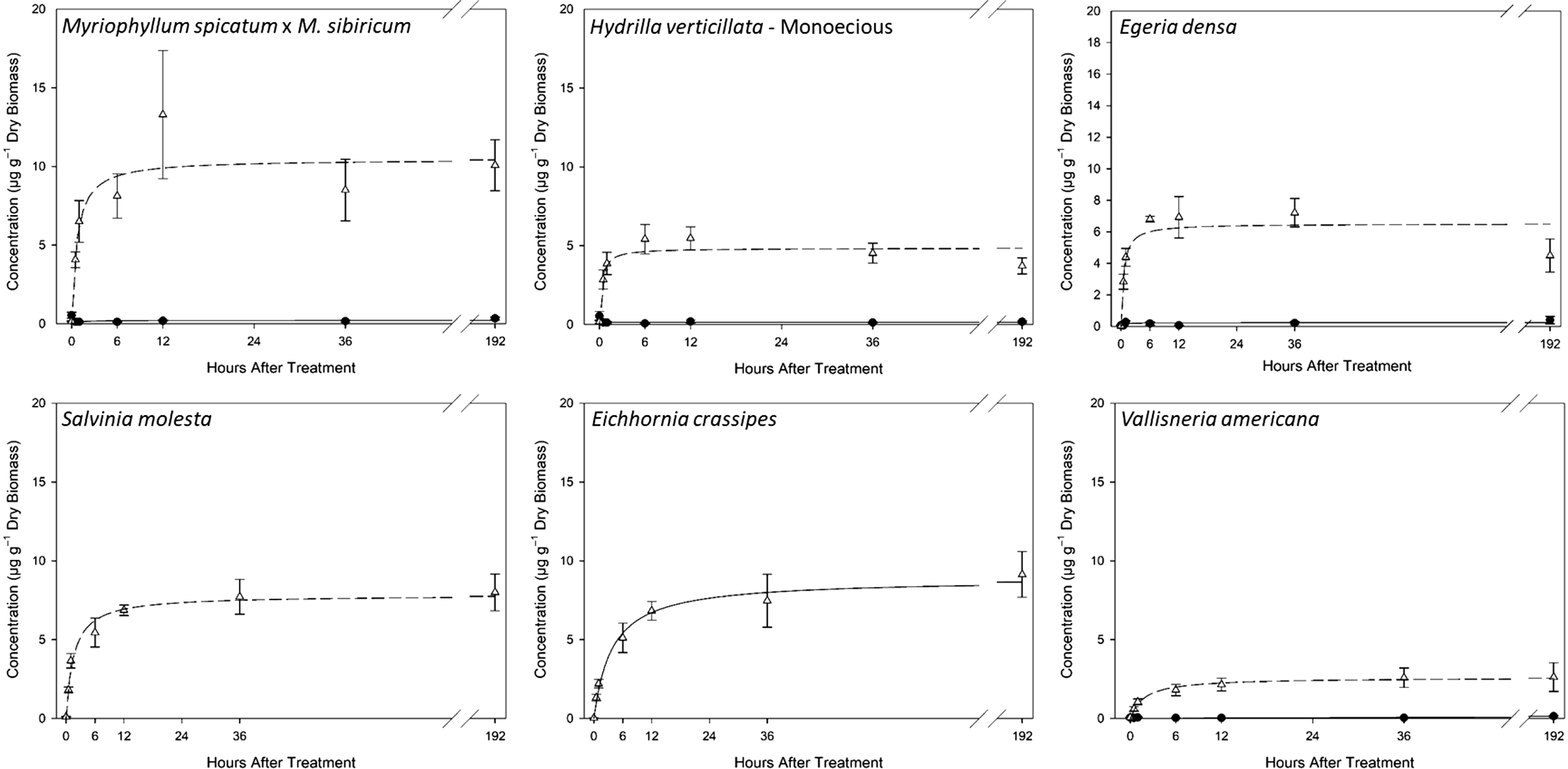
Several studies have indicated that experimental results utilizing dioecious H. verticillata cannot be universally applied to monoecious H. verticillata (McFarland and Barko Reference McFarland and Barko1987; Puri et al. Reference Puri, MacDonald and Haller2007; Spencer and Anderson Reference Spencer and Anderson1986; Steward and Van Reference Steward and Van1987; Sutton et al. Reference Sutton, Van and Portier1992; True-Meadows et al. Reference True-Meadows, Haug and Richardson2016). The aboveground absorption results of this study are yet another example of such. The predicted absorption in monoecious H. verticillata based on our results (A192 = 4.83 µg g−1) is approximately 19% of the absorption predicted for dioecious H. verticillata (A192 = 25.31 µg g−1) (Table 2; Figures 1 and 2). It should be noted that separate sensitivity studies have found florpyrauxifen-benzyl to be highly efficacious for both dioecious and monoecious H. verticillata (Netherland and Richardson Reference Netherland and Richardson2016; Richardson et al. Reference Richardson, Haug and Netherland2016). Beets and Netherland (Reference Beets and Netherland2018) found that doubling the rate of florpyrauxifen-benzyl from 24 to 48 µg L−1 did not increase observed efficacy, nor did increasing the exposure from 24 to 72 h. In this same study, the authors observed a significant decrease in belowground biomass of dioecious H. verticillata (Beets and Netherland Reference Beets and Netherland2018).
Hyperbolic nonlinear regression plots for Myriophyllum spicatum × Myriophyllum sibiricum, monoecious Hydrilla verticillata, Egeria densa, Salvinia molesta, Eichhornia crassipes, and Vallisneria americana. Aboveground data are symbolized with a dashed line for the regression and open triangles for the mean concentration. Belowground data are symbolized with a solid line for the regression and closed circles for the mean concentration. Error bars represent the standard error of the mean. Please note the y axis scales in this figure display a maximum concentration of 20 µg g−1 dry biomass compared with 60 µg g−1 dry biomass in Figure 1.

Results for E. densa (A192 = 6.49 µg g−1), another submersed monocot, indicate a shoot absorption pattern somewhere between that of monoecious H. verticillata and hybrid M. spicatum × M. sibiricum (Table 2). Whereas results for V. americana, a native submersed monocot, indicate a shoot absorption pattern that was lowest of all plant species evaluated in this experiment (A192 = 2.57 µg g−1; PCF192 = 8.89) (Tables 2 and 3; Figure 2). This low level of absorption is consistent with the treatment results indicating no apparent response in relative abundance of V. americana to high levels (48 µg L−1) of florpyrauxifen-benzyl (Sperry et al. Reference Sperry, Leary, Jones and Ferrell2021). Translocation was relatively low for both V. americana and E. densa.
The hyperbolic nonlinear regression model fit the shoot absorption data for N. cristata, the only floating-leaved dicot in this experiment, very well, with an r2 of 0.97 (Table 2; Figure 1). Predicted shoot absorption for N. cristata at 192 HAT (A192 = 20.06 µg g−1) was similar to that of M. spicatum and dioecious H. verticillata (Table 2). Again, this high level of absorption is congruent with the high level of sensitivity to florpyrauxifen-benzyl observed for N. cristata (Netherland and Richardson Reference Netherland and Richardson2016). The highest level of belowground concentration of herbicide observed in this experiment was observed in N. cristata, with A192 of 1.28 µg g−1 (Table 2; Figure 1). Observations of high belowground concentrations of florpyrauxifen-benzyl are consistent with a mesocosm study in which treatment with 24 µg L−1 of the herbicide for 24 to 72 h resulted in significant reductions in belowground biomass (Beets and Netherland Reference Beets and Netherland2018).
Both E. crassipes and S. molesta showed moderate to high levels of absorption, with predicted absorption levels of 8.66 µg g−1 and 7.66 µg g−1, respectively (Table 2; Figure 2). PCF values were also moderate to high at 61 for S. molesta and 55 for E. crassipes (Table 3). As this was an in-water treatment, shoots and roots were not separated to quantify translocation in these floating species.
While predicted shoot absorption values for monocots may appear to be on average lower than those of dicots in this experiment, it should be noted that this apparent difference was not significant in a one-way ANOVA (P = 0.24).
The percentage of herbicide translocated from shoot to root tissue has been low, less than 5% to 10%, in other experiments examining radiolabeled herbicide translocation in submersed aquatic plant species (Vassios et al. Reference Vassios, Nissen, Koschnick and Heilman2017). Evidence of florpyrauxifen-benzyl translocation was observed in all rooted plant species tested, as indicated by the radioactivity measured in isolated root tissues. However, more florpyrauxifen-benzyl translocation was expected than was observed based on the classification of this herbicide as an aryl-picolinate. Aryl-picolinates as a class of herbicides have been shown to translocate well in terrestrial plant tissues (Bromilow et al. Reference Bromilow, Chamerlain and Evans1990; Epp et al. Reference Epp, Alexander, Balko, Buysse, Brewster, Bryan, Daeuble, Fields, Gast, Green, Irvine, Lo, Lowe, Rnega and Richburg2016). One possible explanation for the reduced translocation observed could be due to the application of the formulation blank separate from the application of the active ingredient. This methodology was recommended by the manufacturer; however, it is hard to predict how the chemicals will behave when applied separately in a novel (aqueous) environment. Alternatively, it is possible that the herbicide impacted vascular tissue rapidly enough to reduce movement to belowground tissues, due in part to the small scale at which this experiment took place and the moderate florpyrauxifen-benzyl application rate used.
While synthetic auxin herbicides generally affect dicots more than monocots, sensitivity analyses for florpyrauxifen-benzyl have shown high activity on a select number of monocot invasive aquatic plants (Netherland and Richardson Reference Netherland and Richardson2016; Richardson et al. Reference Richardson, Haug and Netherland2016). Evidence of translocation was observed in all rooted species tested, and moderate to high translocation was observed in N. cristata. High levels of shoot absorption and high plant concentration factors were observed for susceptible species, and reduced absorption levels were absorbed for insensitive species. Finally, low absorption into native V. americana shoot tissues may help to explain florpyrauxifen-benzyl selectivity between this and other Hydrocharitaceae spp. such as H. verticillata. Overall, this study provides additional evidence that florpyrauxifen-benzyl is a good candidate for selective control of several aquatic plant species.
Acknowledgments
The authors would like to acknowledge the members of the North Carolina State University aquatics team for their tireless efforts in the lab, including Tyler Harris, Stephanie Nawrocki, Andrew Howell, Shannon Regan, Kara Foley, Eryn Molloy, Logan Wilson, Taylor Hatfield, and Sarah Roy. Funding for this research was provided by SePRO Corporation. No conflicts of interest have been declared.