1. Introduction
According to the Food and Agriculture Organization of the United Nations in 2011, one-third of world food production was wasted (see [Reference Gustavsson, Cederberg, Sonesson, Otterdijk and Mcybeck14]). In the supply chain, disbursed production occurs in various parts of the process, such as primary production, processing, distribution, retail, and consumption. A point of interest is how retailers order their perishable goods. In essence, if they order too many, there is a high chance that the products will perish and waste will result. A lack of enough inventory may result in lost sales, that is, having empty shelves for part of the day. Corsten and Gruen [Reference Corsten and Gruen10] indicated the worldwide average of out-of-stock (OOS) is 8.3%. A manager's real challenge is to avoid large inventories and frequent OOS for perishable goods. There have been a number of mathematical models proposed for dealing inventory system with perishable products.
Ghare and Schrader [Reference Ghare and Schrader12] introduced the concept of decaying in inventory systems. Several researchers then worked on the perishable inventory theory. See Nahmias [Reference Nahmias19], Raafat [Reference Raafat24], Goyal and Giri [Reference Goyal and Giri13], Karaesmen et al. [Reference Karaesmen, Scheller-Wolf and Deniz18], Bakker et al. [Reference Bakker, Riezebos and Teunter2], Janssen et al. [Reference Janssen, Claus and Sauer16], and Chaudhary et al. [Reference Chaudhary, Kulshrestha and Routroy9] for a detailed review of perishable inventory theory. Nahmias [Reference Nahmias20] gives a great overview of all the types of perishable inventory models. He classified finite lifetime inventories into three major categories according to the nature of lifetimes: decay, obsolescence, or perishability. According to decay or exponential decay, a certain percentage of inventory is lost every planning period. In continuous time, this translates to the size of the inventory decreasing at an exponential rate. A perishable item is one that has constant utility up until an expiration date which may be fixed or random, at which point the utility drops to zero. Packaged foods, dairy products, canned goods, human blood, all pharmaceuticals, and photographic film are all included in this category.
Inventory that is subject to obsolescence is another problem. Obsolescence can be distinguished from perishability by the following characteristics. Obsolescence typically occurs when an item has been superseded by a better version. In this work, we concentrate on inventory models with obsolescence. A portion or all of the inventory on hand may lose its value as a result of obsolescence. Throughout this paper, we only consider the case of sudden obsolescence, which means that items held in inventory have no salvage value and lose all their value suddenly.
The literature contains plenty of examples regarding the obsolescence phenomenon, such as Hadley and Whitin [Reference Hadley and Whitin15] studies about the spare parts management for military aircraft, Joglekar and Lee [Reference Joglekar and Lee17] studies about Swiss watches, music records, and David et al. [Reference David, Greenshtein and Mehrez11] studies about military maps. A number of other sectors are also prone to obsolescence, including avionics and military products, high-tech products, communications, construction, medical devices, transportation, and supply chains (see [Reference Barron4,Reference Chandiran8,Reference Shen and Willems25] and reference therein).
In this paper, we analyze two continuous review inventory systems based on the replenishment policies. In the first model, we assume the  $(s,S)$ policy to replenish the stock and, in the second one, we use the
 $(s,Q)$ policy for stock replenishment. We use the system point (SP) method of level crossing theory, introduced by Brill [Reference Brill5], to derive the governing system of integral equations and these integral equations are used to derive the exact form of stationary probability of the inventory levels. The governing system of equation for the
 $(s,S)$ policy is same as Baron et al. [Reference Baron, Berman and Perry3]. Using the differential equation method, they converted the system of integral equations to four linear equations with four unknowns. Moreover, Baron et al. [Reference Baron, Berman and Perry3] pointed out that “these four linear equations with four unknowns can be solved in closed form (which is too cumbersome to include here).” Instead of using the differential equation method, in the present work, we use the integral equation method, which leads to a nice closed form solutions for the stationary probability for the inventory level. The main advantage of the integral equation method is to extend the same procedure to the
 $(s,Q)$ inventory policy which will be studied in Section 4.
The plan of the article is as follows: In Section 2, we give a brief introduction about the system-point level-crossing (SPLC) method. In Section 3, we provide the complete description of the assumptions of the models. In Section 4, we derive the necessary integral equations for the inventory system  $(s,S)$ replenishment policy, solution procedure for computing the limiting probability distribution and related performance measures. In Section 5, we derive total expected cost rate for the inventory system with
 $(s,Q)$ policy. In Section 6, we give numerical results and some insights from them.
2. Brief introduction of the level crossing method
In this section, we will give a brief introduction to stochastic level crossing using the SP method. In 1975, Brill developed the level crossing method for obtaining probability distributions in stochastic models as part of his PhD thesis. A more general method of SPs was used by him to develop the level crossing method in his thesis (see [Reference Brill5,Reference Brill7]). When analyzing stochastic models using the SPLC, it is often sufficient to use intuitive notions of sample path transitions. For some models, we need to define transitions with more precision. In terms of sample path transitions, downcrossings, upcrossings, and tangents of state space levels are of particular importance.
Consider a continuous time stochastic process  $\{X(t), t\geq 0\}$ with continuous state space
 $E$. Assume that the upward jumps of
 $\{X(t)\}$ occur at Poisson rate
 $\lambda _u$ and downward jumps occur at a Poisson rate
 $\lambda _d$. Assume that these jumps are independent of each other and the state of the system. The corresponding upward and downward jump magnitudes should have cumulative distribution functions (cdfs)
 $B_u$ and
 $B_d$, and the corresponding complementary cdfs should be, respectively,
 $\bar {B}_u$ and
 $\bar {B}_d$. Depending on the model dynamics, other jumps may also be possible depending on the state of the system. Assume that the model parameters are such that the steady-state distribution of
 $X(t)$ exists as
 $t \to \infty$, and let
 $F$ and
 $f$ denote the steady-state cdf and pdf, respectively. In SPLC, the main goal is to obtain integral equation(s) for
 $g$ and then solve for
 $g$ in terms of model input parameters.
First, we construct a typical sample path to deduce the integral equation. A sample path of the process  $\{X(t)\}$ is a single realization of the process over time. Brill refers to the leading point of an evolving sample path as the SP. The sample path value at time point
 $t$ is an outcome of the random variable
 $X(t)$, say
 $Y(t)$.We denote an arbitrary sample path by the function
 $Y(t),\ t \geq 0$, which is a bounded real-valued and right-continuous function. The function
 $Y$ has jump or removable discontinuities on a sequence of strictly increasing time epochs
 $\{\tau _n, n = 0, 1, \ldots,\}$. Without loss of generality, we assume that
 $\tau _0 = 0$. The time epochs
 $\{\tau _n\}$ may represent input or output epochs of the system under consideration.
In SPLC, the state space consists of continuous and discrete states. A continuous state  $\{ y \}$ is characterized by having probability 0. That is
 $P(Y(t) = y) = 0,\ t \geq 0$, and
 $\lim _{t \to \infty } P(Y(t) = y) = 0$. A discrete state or atom is a singleton
 $\{y \}$ characterized by having positive probability. That is
 $P(Y(t) = y) \gt 0$ for some
 $t \geq 0$ and
 $\lim _{t \to \infty } P(Y(t) = y) \gt 0$.
We first examine the continuous states. The following notions will be used in this section.
Definition 1 [Reference Brill6]
A jump downcrossing of level  $y$ occurs at time points
 $t_0 \gt 0$ if
 $\lim _{t\to t_0^{-}}Y(t) \gt y$ and
 $Y(t_0) \leq y$.
Similarly, we can define jump upcrossing of level  $y$.
Let  $D_t^{j}(y)$ and
 $U_t^{j}(y)$, respectively, the total number of jump downcrossing of level
 $y$ during
 $(0,t)$ due to the Poisson rate
 $\lambda _d$ and the total number of jump upcrossing of level
 $y$ during
 $(0,t)$ due to the Poisson rate
 $\lambda _u$. The following results hold.
Theorem 1 [Reference Brill7] Thm. 6.4 p. 325
With probability 1,
 \begin{align} \lim_{t \to \infty} \frac{D_t^{j}(y)}{t} & = \lambda_d \int_{w=y}^{\infty}\bar{B}_d(w-y)g(w)\,dw\quad (\forall y). \end{align}
 \begin{align} \lim_{t \to \infty} \frac{U_t^{j}(y)}{t} & = \lambda_u \int_{w={-}\infty}^{y}\bar{B}_u(y-w)g(w)\,dw \quad (\forall y). \end{align}
Theorem 2 [Reference Brill7] Thm. 6.4 p. 325
 \begin{align} \lim_{t \to \infty} \frac{E(D_t^{j}(y))}{t} & = \lambda_d \int_{w=y}^{\infty}\bar{B}_d(x-w)g(w)dw \quad (\forall y). \end{align}
 \begin{align} \lim_{t \to \infty} \frac{E(U_t^{j}(y))}{t} & = \lambda_u \int_{w={-}\infty}^{y}\bar{B}_u(y-w)g(w)dw \quad (\forall y). \end{align}
For the proofs for the above theorems, we refer Brill [Reference Brill7].
Brill [Reference Brill7] Sect. 1.6.2 p. 16 also proved that for every state space level  $x$ and every sample path, the following conservation law holds. In the long run,
 $$\text{Total downcrossing rate} = \text{Total upcrossing rate}.$$
Using this, and from Eqs. (3) and (4), we get
 \begin{equation} \lambda_d \int_{w=y}^{\infty}\bar{B}_d(w-y)g(w)\,dw = \lambda_u \int_{w={-}\infty}^{y}\bar{B}_u(y-w)g(w)\,dw. \end{equation}
Next, we consider a discrete state  $\{y\} \subset E.$ Let
 $\mathcal {O}_t(\{y\})$ and
 $\mathcal {I}_t(\{y\})$, respectively, denote the number of SP exits and the number of SP entrances of
 $\{y\}$ during
 $(0,t)$. Similar to the continuous states, we have the following rate balance equations for atoms.
Theorem 3 [Reference Brill7, p. 36]
For every atom  $\{y\} \subset E$,
 \begin{align*} \lim_{t \to \infty} \frac{\mathcal{O}_t(\{y\})}{t} & = \lim_{t \to \infty} \frac{\mathcal{I}_t(\{y\})}{t}\quad (\text{with probability } 1).\\ \lim_{t \to \infty} \frac{E(\mathcal{O}_t(\{y\}))}{t} & = \lim_{t \to \infty} \frac{E(\mathcal{I}_t(\{y\}))}{t}. \end{align*}
In addition to the jump downcrossing, a continuous downcrossing is also possible in SPLC. But in the present work, we only have jump downcrossing and jump upcrossing. In the present section, we gave a brief introduction about SPLC for real-valued stochastic process. This may be generalized to vector-valued stochastic process also. For a detailed study of SPLC, we refer Brill [Reference Brill7].
3. Model description
We consider a stochastic inventory system which is monitored continuously for its various events such as demand occurrences, placement and receipt of orders. We assume that the demands arrive according to a Poisson process with rate  $\lambda$ and that the demand sizes are exponentially distributed with parameter
 $\mu$. The obsolescence time is assumed to be exponential with parameter
 $\eta$. At the time of perishability, all the available items are failed and the inventory level drops to zero. We develop two models which are different by the way the stock is replenished.
Model 1: In the first model, we assume
 $(s,S)$ policy to maintain the inventory. That is, we assume that the maximum inventory level is $S$ and when the inventory level drops to or below $s$, we place an order. At the time of replenishment, it reaches its maximum level.
Model 2: In this model, we assume
$(s,Q)$ policy to control the inventory. That is, when the inventory level drops to or below $s$, we place an order for $Q$ items. For this model, we assume that $Q \gt s$.


These are two most common ordering policies in connection with inventory management. These two policies are same, if we assume unit-sized demand and the fixed ordering quantity in model 1 (see [Reference Axsäter1]). But in the current article, the demand size is exponential and the ordering quantity in model 1 is variable, hence these two policies differ. For both models, we assume that the lead time exponential with parameter  $\sigma$. The excess demands that cannot be met from the stock for want of items and those that occur during stock-out are assumed to be lost.
4. Analysis of the $(s,S)$ inventory system

Let  $L(t)$ denote the on-hand inventory level at time
 $t$. From our assumptions, it is clear that the stochastic process
 $\{L(t), t\geq 0\}$ is a continuous time Markov process with state space
 $\Omega =\{w : 0 \leq w \leq S\}$.
Define the cumulative probability function
 $$\Lambda(t,w) =\Pr[L(t)\le w] \quad \text{for } w \in [0, S],\ t \gt0.$$
Since the demand is a compound Poisson process and the lead times and the obsolescence times are independent exponential distributions, the time intervals between these epochs constitute a regenerative process. Therefore, the limiting distribution of  $L(t)$ as
 $t \to \infty$ exists (see [Reference Tijms28]). We are interested in the stationary cumulative distribution function,
 $F(x)=\lim _{t\rightarrow \infty }\Lambda (t,x)$ which has two atoms, one at
 $0$ and another at
 $S$. Let
 $\Pi _0$ and
 $\Pi _S$ denote, respectively, the stationary probability mass at level
 $0$ and
 $S$. The continuous parts of the distribution
 $F(w)$ are defined over the intervals
 $0\lt w \lt s$ and
 $s \leq w \lt S$. The respective density functions are denoted by
 $f_1(w)$ and
 $f_2(w)$, respectively. Thus, we write
 $$F(x)=\left\{\begin{array}{ll} 0, & w\lt 0,\\ \Pi_0, & w=0, \\ \displaystyle\Pi_0 +\int_{0}^{w} f_1(y)\,dy, & 0\lt w\lt s, \\[6pt] \displaystyle\Pi_0 +\int_{0}^{s} f_1(y)\,dy + \int_{s}^{w}f_2(y)\,dy, & s\le w\lt S, \\[6pt] \displaystyle\Pi_0 +\int_{0}^{s} f_1(y)\,dy + \int_{s}^{S}f_2(y)\,dy+\Pi_S = 1, & w \ge S. \end{array}\right.$$
4.1. Integral equations for steady-state pdf for the $(s,S)$ policy

In this subsection, we use SPLC to derive the equations for  $\Pi _0, \Pi _S, f_1(\cdot )$, and
 $f_2(\cdot )$. The following theorem provides the system of integral equations used to compute the steady-state pdf of the model under consideration.
Theorem 4 The system of integral equations for the steady-state probability distribution of the stochastic process  $\{L(t),t\geq 0\}$ is given by
For  $0 \lt w \lt s$,
 \begin{align} & \eta \left(\int_{w}^{s}f_{1}(y)\,dy+\int_{s}^{S}f_{2}(y)\,dy+\Pi_S\right) + \lambda \Pi_Se^{-\mu(S-w)} +\lambda\int_{w}^{s} e^{-\mu (y-w)}f_1(y) \,dy \nonumber\\ & \quad + \lambda \int_{s}^{S}e^{-\mu(y-w)}f_{2}(y)\,dy = \sigma \int_{0}^{w}f_1(y)\,dy + \sigma \Pi_0. \end{align}
For  $s\lt w\lt S,$
 \begin{align} & \eta\left( \int_{w}^{S}f_{2}(y)\,dy +\Pi_S\right)+ \lambda \Pi_Se^{-\mu(S-w)} + \lambda \int_{w}^{S}e^{-\mu(y-w)}f_{2}(y)\,dy\nonumber\\ & \quad = \sigma\int_{0}^{s}f_1(y)\,dy + \sigma \Pi_0. \end{align}
 \begin{align} & (\lambda+\eta) \Pi_S = \sigma \int_{0}^{s} f_1(y) \,dy + \sigma \Pi_0, \end{align}
with the normalizing condition
 \begin{equation} \Pi_S+ \int_{0}^{s}f_1(y) \,dy + \int_{s}^{S}f_2(y) \,dy + \Pi_0 = 1. \end{equation}
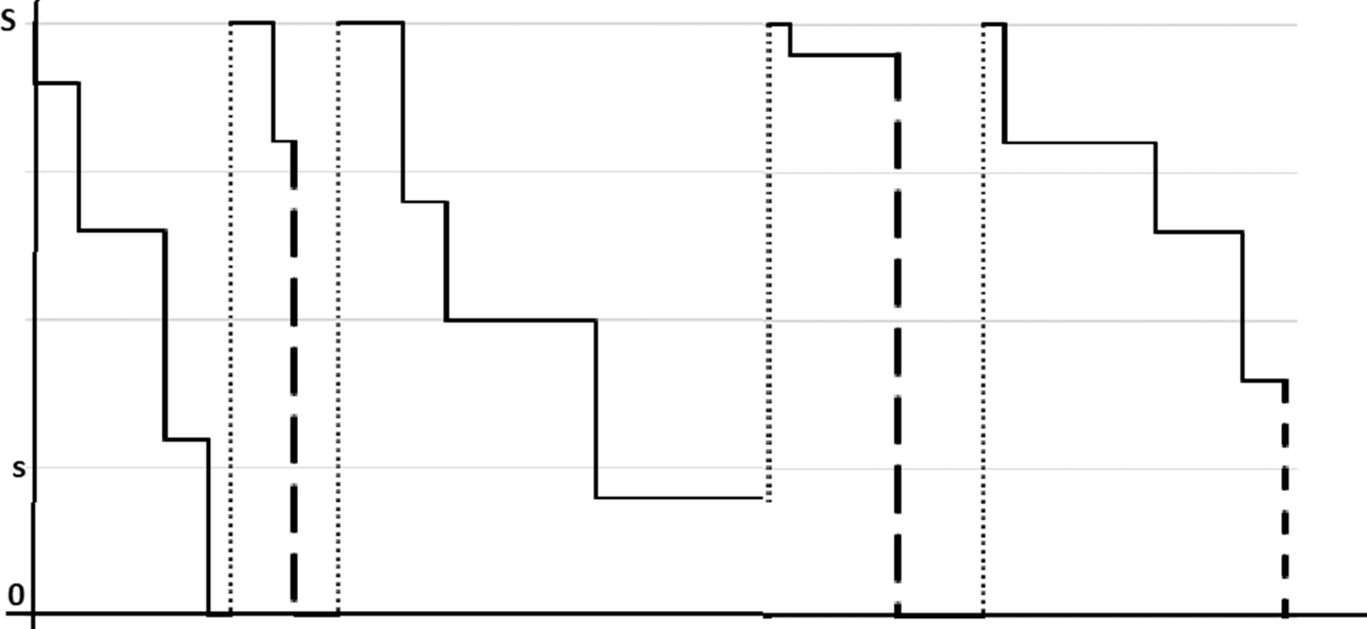
Proof. The stochastic process  $\{L(t),t\geq 0\}$ has sample path similar to Figure 1. From Figure 1, we note that the upcrossing a level is due to replenishment of stock and drowncrossing a level is due to demand and perishability. Let
 $\mathcal {D}_t^{d}, D_t^{p}$, and
 $U_t$, respectively, denote the number of downcrossing of
 $w$ due to demand, the number of downcrossing of
 $w$ due to the obsolescence and number of upcrossing of
 $w$ due to replenishment during the time interval
 $(0,t)$. The SP downcrossing due to demand into level
 $w \in (s,S)$ at rate
 $$\lim_{t\to \infty} \frac{E(\mathcal{D}_t^{d}(w))}{t} = \lambda \Pi_Se^{-\mu(S-w)} + \lambda \int_{w}^{S}e^{-\mu(y-w)}f_{2}(y)\,dy.$$
The SP downcrossing due to obsolescence into level  $w \in (s,S)$ at rate
 $$\lim_{t\to \infty} \frac{E(\mathcal{D}_t^{p}(w))}{t} = \eta\left( \int_{w}^{S}f_{2}(y)\,dy +\Pi_S\right).$$
Hence, the total SP downcrossing the level  $w$ is
 $$\eta\left( \int_{w}^{S}f_{2}(y)\,dy +\Pi_S\right)+ \lambda \Pi_Se^{-\mu(S-w)} + \lambda \int_{w}^{S}e^{-\mu(y-w)}f_{2}(y)\,dy.$$
The SP upcrossing due to replenishment from a level below  $w$ to a level above
 $w$ is
 $$\lim_{t\to \infty} \frac{E(\mathcal{U}_t(w))}{t}=\sigma\int_{0}^{s}f_1(y)\,dy + \sigma \Pi_0.$$
By the theory of SP level crossing (see [Reference Brill7]), the total SP downcrossing is equal to the total SP upcrossing, we have,  $s \lt w \leq S$,
 $$\eta\left( \int_{w}^{S}f_{2}(y)\,dy +\Pi_S\right)+ \lambda \Pi_Se^{-\mu(S-w)} + \lambda \int_{w}^{S}e^{-\mu(y-w)}f_{2}(y)\,dy = \sigma\int_{0}^{s}f_1(y)\,dy + \sigma \Pi_0.$$
Typical sample path for  $(s,S)$ policy. The dotted lines represent replenishment, dashed lines represent obsolescence, and downcrossing lines demand epoch.

Applying a similar SP level-crossing arguments, we derive Eqs. (6) and (8).
4.2. Solution procedure for the $(s,S)$ inventory model

Using the following procedure, we find the solution to the system of integral equations in Theorem 4: First, we differentiate Eq. (7) with respect to  $w$, we get
 $$\lambda \mu \left(e^{({-}S+w) \mu } \Pi_S-\int_S^{w} e^{(w-y) \mu } f_2(y) \, dy\right)=(\eta +\lambda ) f_2(w).$$
The solution of the above integral equation (see [Reference Polyanin and Manzhirov21] p. 144) is
 \begin{equation} f_{2}(w)=\frac{\Pi_S e^{\frac{({-}S+w) \eta \mu }{\eta +\lambda }} \lambda \mu }{\eta +\lambda }.\end{equation}
Substituting the value of  $f_{2}(w)$ in Eq. (6) and differentiate with respect
 $w$, on simplification, we get
 \begin{equation} \lambda \mu \left(e^{-\frac{(S \eta +s \lambda -w (\eta +\lambda )) \mu }{\eta +\lambda }} \Pi_S -\int_s^{w} e^{(w-y) \mu } f_1(y) \, dy\right)=(\eta +\lambda +\sigma ) f_1(w). \end{equation}
Solving the above integral equation, we get
 $$f_{1}(w)= \frac{e^{-\frac{\mu (s \lambda \sigma -w (\eta +\lambda ) (\eta +\sigma )+S \eta (\eta +\lambda +\sigma ))}{(\eta +\lambda ) (\eta +\lambda +\sigma )}} \Pi_S \lambda \mu }{\eta +\lambda +\sigma }.$$
Substitute the value of  $f_1(\cdot )$ and
 $f_2(\cdot )$ in Eqs. (8) and (9) and solving, we get
 \begin{align} \Pi_0 & = \frac{\eta +\lambda -\frac{e^{-\frac{\mu (s \lambda \sigma +S \eta (\eta +\lambda +\sigma ))}{(\eta +\lambda ) (\eta +\lambda +\sigma )}} ({-}1+e^{\frac{s \mu (\eta +\sigma )}{\eta +\lambda +\sigma }}) \lambda \sigma }{\eta +\sigma }}{\eta +\lambda +\sigma +\frac{\lambda \sigma }{\eta }-\frac{e^{\frac{(s-S) \eta \mu }{\eta +\lambda }} \lambda \sigma }{\eta }}. \end{align}
 \begin{align} \Pi_S & = \frac{\eta \sigma }{\eta ^{2}-({-}1+e^{\frac{(s-S) \eta \mu }{\eta +\lambda }}) \lambda \sigma +\eta (\lambda +\sigma )}. \end{align}
4.3. System performance measures
In this subsection, we derive some system performance measures and using these system performance measures we calculate the stationary total expected cost rate.
4.3.1. Expected inventory level
Let  $\zeta _I$ denote the expected inventory level in the steady state. This is given by
 $$\zeta_I = \int_{0}^{s}yf_1(y)\,dy+\int_{s}^{S}yf_2(y)\,dy+S\Pi_S.$$
Substituting the values of  $\Pi _S, f_1(\cdot )$, and
 $f_2(\cdot )$ from (13), (12) and (10), respectively, and on simplification, we get
 \begin{align*} \zeta_I& = \frac{\lambda (-\eta -\lambda +S \eta \mu +e^{\frac{(s-S) \eta \mu }{\eta +\lambda }} (\eta +\lambda -s \eta \mu )) \sigma }{\eta \mu ({-}e^{\frac{(s-S) \eta \mu }{\eta +\lambda }} \lambda \sigma +(\eta +\lambda ) (\eta +\sigma ))}+\frac{S \eta \sigma }{\eta ^{2}-({-}1+e^{\frac{(s-S) \eta \mu }{\eta +\lambda }}) \lambda \sigma +\eta (\lambda +\sigma )}\\ & \quad +\frac{\eta \lambda \sigma (e^{-\frac{\mu (s \lambda \sigma +S \eta (\eta +\lambda +\sigma ))}{(\eta +\lambda ) (\eta +\lambda +\sigma )}} (\eta +\lambda +\sigma )+e^{\frac{(s-S) \eta \mu }{\eta +\lambda }} (-\eta -\lambda -\sigma +s \mu (\eta +\sigma )))}{(\eta +\sigma )^{2} ({-}e^{\frac{(s-S) \eta \mu }{\eta +\lambda }} \lambda \mu \sigma +(\eta +\lambda ) \mu (\eta +\sigma ))}. \end{align*}
4.3.2. Expected obsolescence rate
Let  $\zeta _O$ be the expected obsolescence rate.
 \begin{equation} \zeta_O = \eta\int_{0}^{s}yf_1(y)\,dy+\eta\int_{s}^{S}yf_2(y)\,dy+S\eta\Pi_S = \eta \zeta_I. \end{equation}
4.3.3. Expected reorder rate
Let  $\zeta _R$ be the expected reorder rate.
 \begin{equation} \begin{aligned} \zeta_R & = \eta\int_{s}^{S}f_2(y)\,dy+\eta\Pi_S + \lambda \int_{s}^{S}e^{-\mu(y-s)} f_2(y) \,dy + \lambda e^{-\mu(S-s)} \Pi_S,\\ \zeta_R & = \frac{\eta (\eta +\lambda ) \sigma }{\eta ^{2}-({-}1+e^{\frac{(s-S) \eta \mu }{\eta +\lambda }}) \lambda \sigma +\eta (\lambda +\sigma )}. \end{aligned} \end{equation}
4.3.4. Expected shortage rate
Let  $\zeta _L$ be the expected shortage rate.
 \begin{align*} \zeta_L & = \lambda\Pi_S \int_{x=0}^{\infty}xe^{-\mu (S+x)}\,dx + \lambda\int_{y=s}^{S} f_2(y)\left(\int_{x=0}^{\infty} xe^{-\mu (y+x)} \,dx\right) dy \nonumber \\ & \quad + \lambda \int_{y=0}^{s} f_1(y)\left(\int_{x=0}^{\infty} xe^{-\mu (y+x)} \,dx \right) dy + \lambda \Pi_0 \int_{x=0}^{\infty} xe^{-\mu x} \,dx,\nonumber\\ \zeta_L & = \frac{e^{-\frac{\mu (s \lambda \sigma +S \eta (\eta +\lambda +\sigma ))}{(\eta +\lambda ) (\eta +\lambda +\sigma )}} \eta \lambda ({-}e^{\frac{s \mu (\eta +\sigma )}{\eta +\lambda +\sigma }} \lambda \sigma +e^{\frac{\mu (s \lambda \sigma +S \eta (\eta +\lambda +\sigma ))}{(\eta +\lambda ) (\eta +\lambda +\sigma )}} (\eta +\lambda ) (\eta +\sigma )+\sigma (\eta +\lambda +\sigma ))}{\mu ^{2} (\eta +\sigma ) (\eta ^{2}-({-}1+e^{\frac{(s-S) \eta \mu }{\eta +\lambda }}) \lambda \sigma +\eta (\lambda +\sigma ))}. \end{align*}
4.3.5. Expected total cost
Let  $TC_{1}(s,S)$ denote the total expected cost rate which is given by
 \begin{equation} TC_1(s,S)=c_h\zeta_I+c_r\zeta_R+c_o\zeta_O+c_s\zeta_L, \end{equation}
where  $c_h, c_r,c_o$, and
 $c_s$ denote, respectively, the holding cost per unit time per unit item, the setup cost per order, obsolescence cost per unit time, and shortage cost per unit time.
5. Analysis of the $(s,Q)$ inventory system

Let  $\tilde {L}(t)$ denote the on-hand inventory level at time
 $t$. From the model assumptions, it is clear that the stochastic process
 $\{\tilde {L}(t), t\geq 0\}$ is a continuous-time Markov process with state space
 $\tilde {\Omega } =\{w : 0 \leq w \leq s+Q\}$.
Define the cumulative probability function
 $$\tilde{\Lambda}(t,w) =\Pr[L(t)\le w] \quad \text{for } w \in [0, s+Q],\ t \gt0.$$
Since the demand is a compound Poisson process and the lead times and obsolescence times are independent exponential distributions, the time intervals between these epochs constitute a regenerative process. Therefore, the limiting distribution of  $L(t)$ as
 $t \to \infty$ exists (see [Reference Tijms28]). We are interested in the stationary cumulative distribution function,
 $G(w)=\lim _{t\rightarrow \infty }\tilde {\Lambda }(t,w)$ which has two atoms, one at
 $0$ and another at
 $Q$. Let
 $\Phi _0$ and
 $\Phi _Q$ denote, respectively, the stationary probability mass at level
 $0$ and
 $Q$. The continuous parts of the distribution
 $G(w)$ are defined over the intervals
 $0\lt w \lt s, s \leq w\lt Q$, and
 $Q \lt w \leq Q+s$. The respective density functions are denoted by
 $g_1(w), g_2(w)$, and
 $g_3(w)$. Thus, we write
 $$G(x)=\left\{\begin{array}{ll} 0, & w\lt 0,\\ \Phi_0, & w=0, \\ \displaystyle\Phi_0 +\int_{0}^{w} g_1(y)\,dy, & 0\lt w\lt s, \\[6pt] \displaystyle\Phi_0 +\int_{0}^{s} g_1(y)\,dy + \int_{s}^{w}g_2(y)\,dy, & s\le w\lt Q, \\[6pt] \displaystyle\Phi_0 +\int_{0}^{s} g_1(y)\,dy + \int_{s}^{Q}g_2(y)\,dy + \Phi_Q, & w=Q, \\[6pt] \displaystyle\Phi_0 +\int_{0}^{s} g_1(y)\,dy + \int_{s}^{Q}g_2(y)\,dy + \Phi_Q + \int_{Q}^{w}g_3(y)\,dy, & Q\lt w\lt s+Q, \\[6pt] \displaystyle\Phi_0 +\int_{0}^{s} g_1(y)\,dy + \int_{s}^{Q}g_2(y)\,dy + \Phi_Q + \int_{Q}^{S}g_3(y)\,dy =1, & w\geq s+Q. \end{array}\right.$$
5.1. Integral equations for steady-state pdf for the $(s,Q)$ policy

We apply SPLC to obtain equations for  $\Phi _0, \Phi _Q, g_1(\cdot ),g_2(\cdot )$, and
 $g_3(\cdot )$. The following theorem provides the system of integral equations used to compute the steady-state pdf of the model under consideration.
Theorem 5 The system of integral equations for the steady-state probability distribution of the stochastic process  $\{\tilde {L}(t),t\geq 0\}$ is given by
 \begin{equation} (\lambda+\eta) \Phi_Q = \sigma \Phi_0. \end{equation}
For  $0 \lt w \lt s$,
 \begin{align} & \eta \left(\int_{w}^{s}g_{1}(y)\,dy+\int_{s}^{Q}g_{2}(y)\,dy+\Phi_Q+\int_{Q}^{s+Q}g_{3}(y)\,dy\right) + \lambda \Phi_Qe^{-\mu(Q-w)}\nonumber\\ & \qquad + \lambda\int_{w}^{s} e^{-\mu (y-w)}g_1(y) \,dy + \lambda \int_{s}^{Q}e^{-\mu(y-w)}g_{2}(y)\,dy + \lambda \int_{Q}^{s+Q}e^{-\mu(y-w)}g_{3}(y)\,dy\nonumber\\ & \quad = \sigma \int_{0}^{w}g_1(y)\,dy + \sigma \Phi_0. \end{align}
For  $s\lt w\lt Q,$
 \begin{align} & \eta \left(\int_{w}^{Q}g_{2}(y)\,dy+\Phi_Q+\int_{Q}^{s+Q}g_{3}(y)\,dy\right) + \lambda \Phi_Qe^{-\mu(Q-w)} \nonumber\\ & \quad + \lambda \int_{w}^{Q}e^{-\mu(y-w)}g_{2}(y)\,dy + \lambda \int_{Q}^{s+Q}e^{-\mu(y-w)}g_{3}(y)\,dy = \sigma\int_{0}^{s}g_1(y)\,dy + \sigma \Phi_0. \end{align}
For  $Q\lt w\lt s+Q,$
 \begin{equation} \eta \left(\int_{w}^{s+Q}g_{3}(y)\,dy\right) + \lambda \int_{w}^{s+Q}e^{-\mu(y-w)}g_{3}(y)\,dy = \sigma\int_{w-Q}^{s}g_1(y)\,dy, \end{equation}
with the normalizing condition
 \begin{equation} \Phi_Q+ \int_{0}^{s}g_1(y) \,dy + \int_{s}^{Q}g_2(y) \,dy + \int_{Q}^{s+Q}g_3(y) \,dy + \Phi_0 = 1, \end{equation}
and the boundary condition is
 \begin{equation} g_1(0)= \sigma \Phi_0. \end{equation}
Proof. The balance equations are derived using the arguments similar to Theorem 1. To derive the boundary condition, we note that all hits at level 0 are due to sample path which has continuous entrances into level  $\{0\}$ from
 $(0,s+Q]$. Since every hit from above of each level
 $x \gt0$ is a continuous downcrossing of level
 $x$, the hit rate of level 0 from above is the entrance rate of state
 $\{0\}$, namely
 $g_1(0)$. We note that the SP egress rate from level 0 above is the exit rate from discrete state
 $\{0\}$. The rate
 $\sigma \Phi _0$ gives the rate at which an order arrive when the inventory level is 0. Equating the exit and entrance rate of the atom
 $\{0\}$ yields the boundary condition.
5.2. Solution procedure for the $(s,Q)$ inventory model

In order to solve the integral equations derived in Theorem 5, we use the following method. First, we differentiate Eq. (19) with respect to  $w$, which gives
 \begin{align} & \lambda \mu \left(\int_w^{s} g_{1}(y) e^{\mu (w-y)} \, dy+\int_s^{Q} {g_2}(y) e^{\mu (w-y)} \, dy+\int_Q^{Q+s} {g_3}(y) e^{\mu (w-y)} \, dy+ {\Phi_Q} e^{\mu (w-Q)}\right)\nonumber\\ & \quad ={g_{1}}(w) (\eta +\lambda +\sigma ). \end{align}
Equating Eqs. (18) and (23), we get
 \begin{align} & \eta \mu \left(\int_{w}^{s}g_{1}(y)\,dy+\int_{s}^{Q}g_{2}(y)\,dy+\Phi_Q+\int_{Q}^{s+Q}g_{3}(y)\,dy\right) + {g_1}(w) (\eta +\lambda +\sigma )\nonumber\\ & \quad = \sigma \mu \int_{0}^{w}g_1(y)\,dy + \sigma\Phi_0. \end{align}
Differentiate Eq. (24) with respect to  $w$, we get
 \begin{equation} \mu (\eta +\sigma) g_1(w)=(\eta +\lambda +\sigma ) g_1'(w). \end{equation}
Solving the above differential equation with boundary condition (22), we have
 \begin{equation} g_1(w)= e^{\frac{w \mu (\eta +\sigma )}{\eta +\lambda +\sigma }} \Phi_0 \sigma. \end{equation}
Next, differentiate Eq. (20) with respect to  $w$, and substitute
 $g_1(w)$, we get
 \begin{equation} \Phi_0 \sigma ^{2} e^{\frac{\mu (\eta +\sigma ) (w-Q)}{\eta +\lambda +\sigma }}=(\eta +\lambda ) g_3(w) + \lambda\mu \int_{Q+s}^{w} e^{\mu (w-y)} g_3(y) \,dy. \end{equation}
Solving the above integral equation, we get
 \begin{equation} g_3(w)={-}\frac{e^{-\frac{(Q-w) \mu (\eta +\sigma )}{\eta +\lambda +\sigma }} \Phi_0 \sigma (-\sigma -({-}1+e^{\frac{(Q+s-w) \lambda \mu \sigma }{(\eta +\lambda ) (\eta +\lambda +\sigma )}}) (\eta +\lambda +\sigma ))}{\eta +\lambda }. \end{equation}
Substituting the values of  $g_1(w)$ and
 $g_3(w)$ in Eq. (19) and differentiate the resulting equation, we have
 \begin{align} & \lambda \mu \Phi_Q e^{-\mu (Q-w)} - \frac{1}{\mu}\left(\Phi_0 \sigma (\eta +\lambda +\sigma ) e^{\lambda \mu ({-}Q) (\frac{1}{\eta +\lambda +\sigma }+\frac{1}{\eta +\lambda })}\right.\nonumber\\ & \qquad \times \left.\left(\mu e^{\mu (-\frac{Q (\eta +\sigma )}{\eta +\lambda +\sigma }+\frac{\lambda Q}{\eta +\lambda }+w)} -\mu e^{(\mu (\frac{\lambda Q}{\eta +\lambda +\sigma }+\frac{\lambda s \sigma -\eta Q (\eta +\lambda +\sigma )}{(\eta +\lambda ) (\eta +\lambda +\sigma)}+w))}\right)\right) \nonumber\\ & \quad = \lambda \mu \int_Q^{w} g_2(y) e^{-\mu(y-w)}\, dy +(\lambda+ \eta)g_2(w). \end{align}
Solving the above integral equation, we get
 \begin{equation} g_2(w)=\frac{e^{\frac{({-}Q+w) \eta \mu }{\eta +\lambda }} (\Phi_Q \lambda \mu +({-}1+e^{\frac{s \lambda \mu \sigma }{(\eta +\lambda ) (\eta +\lambda +\sigma )}}) \Phi_0 \sigma (\eta +\lambda +\sigma ))}{\eta +\lambda }. \end{equation}
From Eq. (17), we get
 \begin{equation} \Phi_Q =\sigma \Phi_0/(\lambda +\eta ). \end{equation}
Substituting  $\Phi _Q, g_1(\cdot ),g_2(\cdot )$, and
 $g_3(\cdot )$ on the normalizing condition (21), and solving we get
 \begin{equation} \Phi_0= 1/\Gamma, \end{equation}
where
 \begin{align*} \Gamma& =\left(1+\frac{1}{\eta (\eta +\lambda ) \mu }e^{-\frac{Q \mu (\eta +\sigma )}{\eta +\lambda +\sigma }} \sigma \left(e^{\frac{Q \mu (\eta +\sigma )}{\eta +\lambda +\sigma }} (\eta +\lambda ) (-\eta -\lambda +\mu -\sigma )\right.\right.\nonumber\\ & \quad +e^{\frac{(Q+s) \mu (\eta +\sigma )}{\eta +\lambda +\sigma }} (\eta +\lambda ) (\eta +\lambda +\sigma )- e^{\frac{\mu (\frac{Q \lambda \sigma }{\eta +\lambda }+s (\eta +\sigma ))}{\eta +\lambda +\sigma }} (\eta +\lambda ) (\eta +\lambda +\sigma )\nonumber\\ & \quad \left.\left.+\,e^{\frac{\mu (s \eta +\frac{Q \lambda \sigma }{\eta +\lambda +\sigma })}{\eta +\lambda }} (\eta ^{2}+\eta (2 \lambda +\sigma )+\lambda (\lambda -\mu +\sigma ))\right)\right). \end{align*}
5.3. System performance measures
In this subsection, we derive some system performance measures and using these system performance measures we calculate the stationary total expected cost rate.
5.3.1. Expected inventory level
Let  $\psi _I$ denote the expected inventory level in the steady state. This is given by
 \begin{align*} \psi_I & = \int_{0}^{s}yg_1(y)\,dy+\int_{s}^{Q}yg_2(y)\,dy+Q\Phi_Q+\int_{Q}^{s+Q}yg_3(y)\,dy,\\ \psi_I & = \Phi_0 \sigma \left(\frac{Q}{\eta +\lambda }-\frac{(\eta +\lambda -Q \eta \mu -e^{\frac{({-}Q+s) \eta \mu }{\eta +\lambda }} (\eta +\lambda -s \eta \mu )) (\frac{\lambda \mu }{\eta +\lambda }+({-}1+e^{\frac{s \lambda \mu \sigma }{(\eta +\lambda ) (\eta +\lambda +\sigma )}}) (\eta +\lambda +\sigma ))}{\eta ^{2} \mu ^{2}}\right.\\ & \quad -\frac{1}{\eta ^{2} \mu ^{2} (\eta +\sigma )^{2}}e^{-\frac{Q \mu (\eta +\sigma )}{\eta +\lambda +\sigma }} (\eta +\lambda +\sigma ) \left(e^{\frac{\mu (Q \eta +\frac{(Q+s) \lambda \sigma }{\eta +\lambda +\sigma })}{\eta +\lambda }} (-\lambda +\eta ({-}1+Q \mu )) (\eta +\sigma )^{2}\right.\\ & \quad -e^{\frac{Q \mu (\eta +\sigma )}{\eta +\lambda +\sigma }} \eta ^{2} (-\lambda +\eta ({-}1+Q \mu )+({-}1+Q \mu ) \sigma )-e^{\frac{(Q+s) \mu (\eta +\sigma )}{\eta +\lambda +\sigma }} \sigma ({-}2 \eta \lambda +\eta ^{2} ({-}1+(Q+s) \mu )\\ & \quad \left.-\lambda \sigma +\eta ({-}1+(Q+s) \mu ) \sigma ) )+\frac{(\eta +\lambda +\sigma ) (\eta +\lambda +\sigma +e^{\frac{s \mu (\eta +\sigma )}{\eta +\lambda +\sigma }} (-\eta -\lambda -\sigma +s \mu (\eta +\sigma )))}{\mu ^{2} (\eta +\sigma )^{2}} \right). \end{align*}
5.3.2. Expected obsolescence rate
Let  $\psi _O$ be the expected obsolescence rate which is given by
 \begin{equation} \psi_O =\eta\int_{0}^{s}yg_1(y)\,dy+\eta\int_{s}^{Q}yg_2(y)\,dy+Q\eta\Phi_Q+\eta\int_{Q}^{s+Q}yg_3(y)\,dy. \end{equation}
5.3.3. Expected reorder rate
Let  $\psi _R$ be the expected reorder rate.
 \begin{align*} \psi_R & = \eta\int_{s}^{Q}g_2(y)\,dy+ \eta\int_{Q}^{s+Q}g_3(y)\,dy+Q\eta\Phi_Q+ \lambda \int_{s}^{Q}e^{-\mu(y-s)} g_2(y) \,dy \\ & \quad + \lambda \int_{Q}^{s+Q}e^{-\mu(y-s)} g_3(y) dy +\lambda e^{-\mu(Q-s)}\Phi_Q,\nonumber\\ \psi_R & = \Phi_0 \sigma \left(\frac{\eta }{\eta +\lambda }+\frac{e^{({-}Q+s) \mu } \lambda }{\eta +\lambda }+\frac{e^{\frac{\mu ({-}Q (\eta +\lambda ) (\eta +2 \lambda +\sigma )+s (\eta ^{2}+\eta (2 \lambda +\sigma )+\lambda (\lambda +2 \sigma )))}{(\eta +\lambda ) (\eta +\lambda +\sigma )}} (e^{\frac{Q \lambda \mu }{\eta +\lambda +\sigma }}-e^{\frac{\lambda \mu (Q (\eta +\lambda )-s \sigma )}{(\eta +\lambda ) (\eta +\lambda +\sigma )}}) (\eta +\lambda +\sigma )}{\mu }\nonumber \right.\\ & \quad +\frac{e^{-\frac{Q \mu (\eta +\sigma )}{\eta +\lambda +\sigma }} (\eta +\lambda +\sigma ) (e^{\frac{Q \mu (\eta +\sigma )}{\eta +\lambda +\sigma }} \eta +e^{\frac{(Q+s) \mu (\eta +\sigma )}{\eta +\lambda +\sigma }} \sigma -e^{\frac{\mu (s \lambda \sigma +Q (\eta +\lambda ) (\eta +\sigma ))}{(\eta +\lambda ) (\eta +\lambda +\sigma )}} (\eta +\sigma ))}{\mu (\eta +\sigma )}\nonumber\\ & \quad -\frac{({-}1+e^{-\frac{(Q-s) \eta \mu }{\eta +\lambda }}) (\frac{\lambda \mu }{\eta +\lambda }+({-}1+e^{\frac{s \lambda \mu \sigma }{(\eta +\lambda ) (\eta +\lambda +\sigma )}}) (\eta +\lambda +\sigma ))}{\mu }\nonumber\\ & \quad + \left.\frac{e^{-\frac{(Q-s) (2 \eta +\lambda ) \mu }{\eta +\lambda }} (e^{(Q-s) \mu }-e^{\frac{(Q-s) \eta \mu }{\eta +\lambda }}) (\frac{\lambda \mu }{\eta +\lambda }+({-}1+e^{\frac{s \lambda \mu \sigma }{(\eta +\lambda ) (\eta +\lambda +\sigma )}}) (\eta +\lambda +\sigma ))}{\mu }\right). \end{align*}
5.3.4. Expected shortage rate
Let  $\psi _L$ be the expected shortage rate.
 \begin{align*} \psi_L & = \lambda\Phi_Q \int_{x=0}^{\infty}xe^{-\mu (Q+x)}\,dx + \lambda\int_{y=s}^{Q} g_2(y)\left(\int_{x=0}^{\infty} xe^{-\mu (y+x)} \,dx\right) dy \nonumber \\ & \quad + \lambda \int_{y=0}^{s} g_1(y)\left(\int_{x=0}^{\infty} xe^{-\mu (y+x)} \,dx \right) dy +\lambda\int_{y=Q}^{s+Q} g_3(y)\left(\int_{x=0}^{\infty} xe^{-\mu (y+x)} \,dx\right) dy\nonumber\\ & \quad + \lambda \Phi_0 \int_{x=0}^{\infty} xe^{-\mu x} dx,\nonumber\\ \psi_L & = \frac{\Phi_0}{\mu ^{3}} \left(\lambda \mu +\frac{e^{{-}Q \mu } \lambda \mu \sigma }{\eta +\lambda }-({-}1+e^{-\frac{s \lambda \mu }{\eta +\lambda +\sigma }}) \sigma (\eta +\lambda +\sigma )\nonumber\right.\\ & \quad +\left.e^{-(Q+\frac{s \lambda }{\eta +\lambda }) \mu } (e^{\frac{Q \lambda \mu }{\eta +\lambda }}-e^{\frac{s \lambda \mu }{\eta +\lambda }}) \sigma \left(\frac{\lambda \mu }{\eta +\lambda }+({-}1+e^{\frac{s \lambda \mu \sigma }{(\eta +\lambda ) (\eta +\lambda +\sigma )}}) (\eta +\lambda +\sigma )\right)\right). \end{align*}
5.3.5. Expected total cost
Let  $TC_{2}(s,Q)$ denote the total expected cost rate which is given by
 \begin{equation} TC_2(s,Q)=c_h\psi_I+c_r\psi_R+c_o\psi_O+c_s\psi_L, \end{equation}
where  $c_h, c_r,c_o$, and
 $c_s$ denote, respectively, the holding cost per unit time per unit item, the setup cost per order, obsolescence cost per unit time, and shortage cost per unit time.
6. Numerical illustrations
The objectives of this section is twofold: we first study the effect of input parameters on the performance measures. Next, we will numerically investigate the optimization of the total cost functions for  $(s,S)$ and
 $(s,Q)$ policies and we numerically justify the best policy.
6.1. Influence of input parameters on the system performance measures
We will examine the influence of input parameters on the system performance measures in this subsection. The numerical work is performed using Wolfram Mathematica 12.2. As a first step in studying the impact of input parameters on the system performance measures of the  $(s,S)$ inventory system, we set the following parameters and values:
 $\sigma = 0.2$;
 $\mu = 1$;
 $\lambda = 10$;
 $\eta = 0.03$;
 $s = 126$;
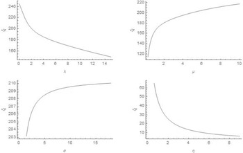
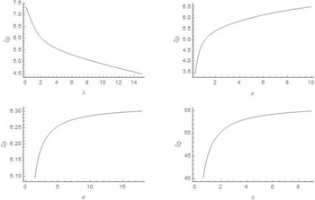
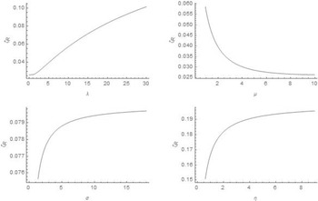
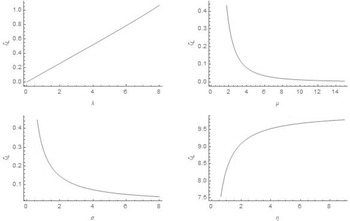
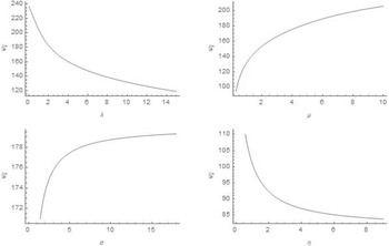
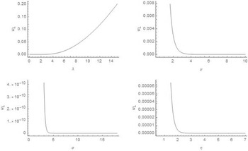
 $S = 282$. Figures 2–5 illustrate how system parameters affect the specific performance measures. There are four subfigures in each figure. We fix the other parameters and values and change only one parameter on the subfigure that is plotted on the
 $x$-axis of the corresponding subfigure. This leads to the following results.
• As the demand rate increases, the mean inventory level
$\zeta _I$ and the mean obsolescence rate $\zeta _O$ decrease while the mean reorder rate $\zeta _R$ and the mean shortage rate $\zeta _L$ increase. The shortage rate increases linearly with demand. For small values of $\lambda$, the increasing rate of mean reorder rates is low, but for high values of $\lambda$, it is high.• When the demand size parameter
$\mu$ increases, $\zeta _I$ and $\zeta _O$ increase and $\zeta _R$ and $\zeta _L$ decrease.• When
$\sigma$ increases, $\zeta _L$ decreases and the remaining performance measures are increase. When $\eta$ increases $\zeta _I$ decreases and the remaining performance measures are increase.


Influence of input parameters on the expected inventory level.

Effect of input parameters on the expected obsolescence rate.

Sensitivity of input parameters on the expected reorder rate.

Influence of input parameters on the expected shortage rate.

Next, we will study the influence of system parameters on the system performance measures of the  $(s,Q)$ inventory system. For this, we first consider the following values for the input parameters,
 $\sigma = 0.2$;
 $\mu = 1$;
 $\lambda = 10$;
 $\eta = 0.03$;
 $s = 82$;
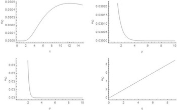
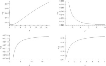
 $Q = 180$. From Figures 6–9, we observe the following:
• The behaviour of the mean inventory level
$\psi _I,\psi _L$, and $\psi _R$ are similar to the model 1.• For the expected obsolescence rate
$\psi _O$ case, it increases with $\lambda$ and $\eta$ and decreases with increase in $\mu$ and $\sigma$. We also note that the $\psi _O$ increase linearly with $\eta$.


Influence of input parameters on the expected inventory level.

Effect of input parameters on the expected obsolescence rate.

Sensitivity of input parameters on the expected reorder rate.

Influence of input parameters on expected shortage.

6.2. Optimal cost analysis
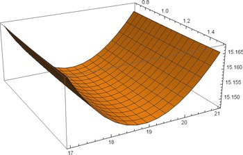
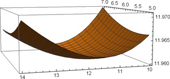
In this subsection, we will investigate the cost functions numerically. Since the cost functions derived in the previous sections are complex, it is not practical to establish its convexity in an analytical sense by using the calculus method. Researches use a wide range of meta-heuristic algorithms to study such cost functions, including genetic algorithms, ant colony optimizations, etc. In our study, we use differential evolution (DE), a meta-heuristic search algorithm that optimizes a problem by iteratively improving a candidate solution over time. Price [Reference Price22] developed the Genetic Annealing algorithm that lead to DE. DE has proven to be a powerful global optimizer since it was conceived. Despite using relatively low resources, this optimization algorithm achieves the real optimum. For a detailed overview of DE, see Price et al. [Reference Price, Storn and Lampinen23]. In order to find optimal values, we use Wolfram Mathematica 12.2 DE solver. To ensure the solution provided by Mathematica is optimal, we plot the objective function in the neighborhood of the values given by Mathematica. The three-dimensional plots of the cost functions are shown in Figures 10 and 11 which show that convex (possibly local) nature of the cost functions.
A typical three-dimensional plot of cost function.  $\sigma = 3.6$,
 $\mu = 0.35$,
 $\lambda = 0.15$,
 $\eta = 0.25$,
 $c_h = 0.01$,
 $c_r = 50$,
 $c_s = 15$,
 $c_o = 0.2$,
 $s^{*}=0.972071$,
 $S^{*}=18.9006$,
 $TC_{1}(s^{*},S^{*})=15.1472$.

A typical three-dimensional plot of cost function.  $\sigma = 3.6$,
 $\mu = 0.35$,
 $\lambda = 0.015$,
 $\eta = 0.25$,
 $c_h = 0.01$,
 $c_r = 50$,
 $c_s = 15$,
 $c_o = 0.2$,
 $s^{*}=6.0878$,
 $Q^{*}=11.8799$,
 $TC_2(s^{*},Q^{*})=11.9599$.

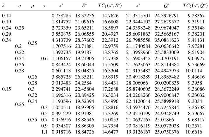
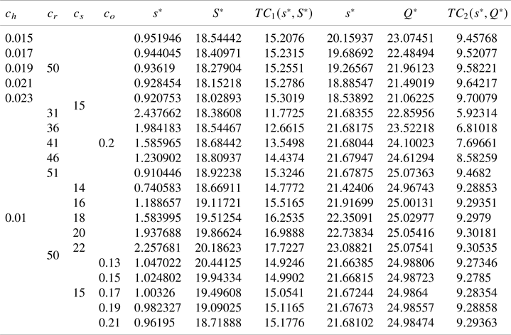
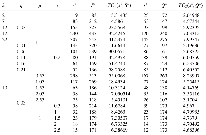
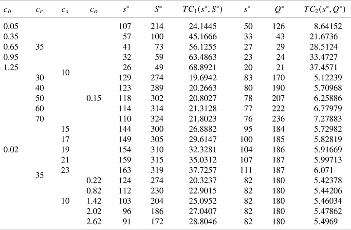
Sensitivity analysis of the optimal values perturbing different parameters and values are presented in Tables 1–4. For Tables 1 and 2, we allow the optimal values of  $(s, S)$ and
 $(s,Q)$ to be positive and real. But in Tables 3 and 4, we restrict the decision variable to be integer.
Influence of parameters on optimal values.

 $c_h = 0.01, c_r = 50, c_s = 15, c_o = 0.2$.
Sensitivity of cost values to optimal values.

 $\lambda = 0.15, \mu = 0.35, \eta = 0.25, \sigma = 0.6$.
Influence of parameters on optimal values.

 $c_h = 0.02, c_r = 35, c_s = 10, c_o = 0.15$.
Sensitivity of cost values to optimal values.

 $\lambda = 10, \mu = 1, \eta = 0.03, \sigma = 0.2$.
We observe the following from the tables of the  $(s,S)$ policy inventory model:
• The optimal inventory level
$S^{*}$ and the optimal reorder point $s^{*}$ increase with the arrival rate $\lambda$ and decrease with increase in $\eta, \ \mu$, and $\sigma$. The optimal cost increase when $\lambda$ and $\eta$ increase and decrease with increase in $\mu$ and $\sigma$.• As
$c_s$ increases, the optimal reorder point $s^{*}$ also increases, and as $c_h, c_s$, and $c_o$ increase, $s^{*}$ decreases.• The optimal maximum stock level
$S^{*}$ increase with $c_r$ and $c_s$ and decrease when $c_h$ and $c_o$ increase.


We observe the following from the tables of the  $(s,Q)$ inventory policy:
• The optimal reorder point
$s^{*}$ increase with the demand rate $\lambda$ and the obsolescence parameter $\eta$ and decrease with increase in the lead time parameter $\sigma$ and the demand size quantity parameter $\mu$. The optimal order quantity $Q^{*}$ increase with $\lambda$ and $\sigma$ and decrease with increase in $\eta$ and $\mu$. As $\lambda$ and $\mu$ increase, the optimal cost increase and the optimal cost decrease when $\mu$ and $\sigma$ increase.• As
$c_s$ increases, the optimal reorder point $s^{*}$ also increases, and as $c_h, c_s$, and $c_o$ increase, $s^{*}$ decreases.• The optimal order quantity
$Q^{*}$ increase with $c_r, c_o$, and $c_s$ and decrease when $c_h$ increases.• But the integer-valued decision variables, the influence of
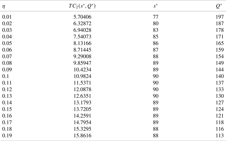
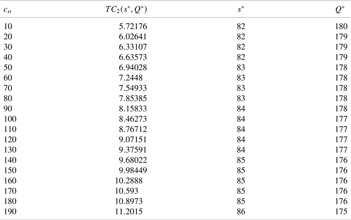
$c_o$ on $s^{*}$ and $Q^{*}$ is very low compared to the corresponding continuous decision variable model (see Tables 5 and 6).


Effect of the obsolescence rate on optimal values for  $(s,Q)$ policy.

 $\lambda = 10, \mu = 1, \sigma = 0.2, c_h = 0.02, c_r = 35, c_s = 10, c_o = 0.15$.
Influence of the obsolescence cost on optimal values for  $(s,Q)$ policy.

 $\lambda = 10, \mu = 1, \sigma = 0.2,\eta =0.03, c_h = 0.02,c_r = 35, c_s = 10$.
For both the replenishment policies, the optimal costs increase when the  $c_h,c_r,c_s$, and
 $c_o$ increase. In both replenishment policies, integer-valued decision variables exhibit the same behavior as real-valued decision variables, except when obsolescence parameters influence
 $s^{*}$ for the
 $(s,Q)$ inventory policy. The optimal reorder point
 $s^{*}$ behaves as a convex function of
 $\eta$ for the
 $(s,Q)$ policy inventory model (see Table 5).
6.3. Management insights of the models
Using our analysis and results, we can gain several insights about the managing inventory system with obsolescence. We have to pointed out that in the literature of the continuous review inventory system, the continuous review  $(s,S)$ (with variable lost size) inventory model is more suitable for the vendor managed inventory system and the continuous review
 $(s,Q)$ (with fixed lot size) inventory is more suitable for the retailer managed inventory system. From tables, we observe:
• Despite the fact that the
$(s,S)$ inventory policy is widely used in vendor managed inventory systems and the $(s,Q)$ inventory policy is used in retailer managed inventory systems, the numerical results indicate that $(s,Q)$ policy will result in the lowest cost.• As a arrival rate increases the optimal reorder point in both models increase and the optimal inventory level in model 1 and optimal ordering quantity in model 2 increase. The optimal inventory level in model 1 grows slowly compared to optimal ordering quantity in model 2 when the arrival rate increase.
• As the time to obsolescence increases
$s^{*}$ and $S^{*}$ increase in the first model and $Q^{*}$ increases and $s^{*}$ decreases in the second model.


7. Conclusion and future works
In this article, we have studied the effect of obsolescence on two continuous review inventory systems with positive lead times. We provided closed-form expressions for the total expected cost rate and analyzed them numerically. In both models, we have assumed the exponentially distributed demand size. These models may be suitable to analyze the behaviour of the inventory system of continuous type (fluid type inventory), such as chemical products and 3D-printing inks. We used SPLC and the integral equation method to get the closed-form expressions.
The SPLC method is one of the effective method to model continuous type inventory models. Due to the deterministic nature of lifetimes of perishable items and the stochastic nature of other parameters, using other methods to analyze the inventory level may be more complex. As a result, the SPLC method can be used to analyze continuous type inventory with perishable items but we leave their investigation for future work. We have also restricted our work to lost sales case only. Including backlog may give some complication. Also for the second model, we allowed atmost one is pending at a time. One can also relax this assumption for the obsolescence inventory model.
Acknowledgments
The research of Ms. K. Preethi is supported by the INSPIRE Fellowship, New Delhi, research award No. DST/INSPIRE Fellowship/[IF160570]. The authors thank DST-PURSE program of MKU for providing Wolfram Mathematica software.