2. STROBE PRINCIPLE

The incoming GNSS signal is digitalised before being processed in the tracking loop. Additionally, front-end filtering is also essential for enhancing the noise resistance. In this paper, the analysis is still conducted in an analogue way without considering the navigation message bit flip. The complex signal being filtered by the front-end filter can be described as follows:

(1)$$\tilde {s}(t)=\sqrt {2C} \tilde {X}(t-\tau _0)\exp \{ {j(\omega_0 t+\varphi_0 )} \} +\tilde {n}(t)$$

where ś(t) is the filtered signal mixed with the filtered white Gaussian noise ñ(t) of N ₀ power spectrum density, with C denoting the signal power, τ ₀ denoting the code phase, φ ₀ denoting the carrier phase and ω ₀ representing the carrier frequency accounting for the Doppler effect. The baseband signal X(t) = c(t) is a PRN code sequence for a BPSK signal, whereas X(t) = c(t) e(t) is composed of both a PRN code sequence and a sub-carrier sequence for BOC and MBOC signals. No dynamics are considered, and the frequency is assumed to be known, thus the in-phase (I-branch) and out-of-phase (Q-branch) correlation outputs can be given by a complex form as:

(2)$$\begin{align} U_{\tilde {X}X} (\varepsilon)&= I_{\tilde {X}X} (\varepsilon )+jQ_{\tilde {X}X} (\varepsilon )\nonumber \\ & = \frac{1}{T}\left\{ \int_0^T \sqrt {2C} \tilde {X}(t-\tau_0 )X(t- {\mathop{\tau} \limits^{\frown}}_0) +\tilde {n}(t)X(t-{\mathop{\tau} \limits^{\frown}}_0 )dt \right\}\exp (j\varphi _e )\nonumber \\ & = \sqrt {2C} R_{\tilde {X}X} (\varepsilon )\exp (j\varphi _e )+N_{\tilde {X}X} \end{align}$$

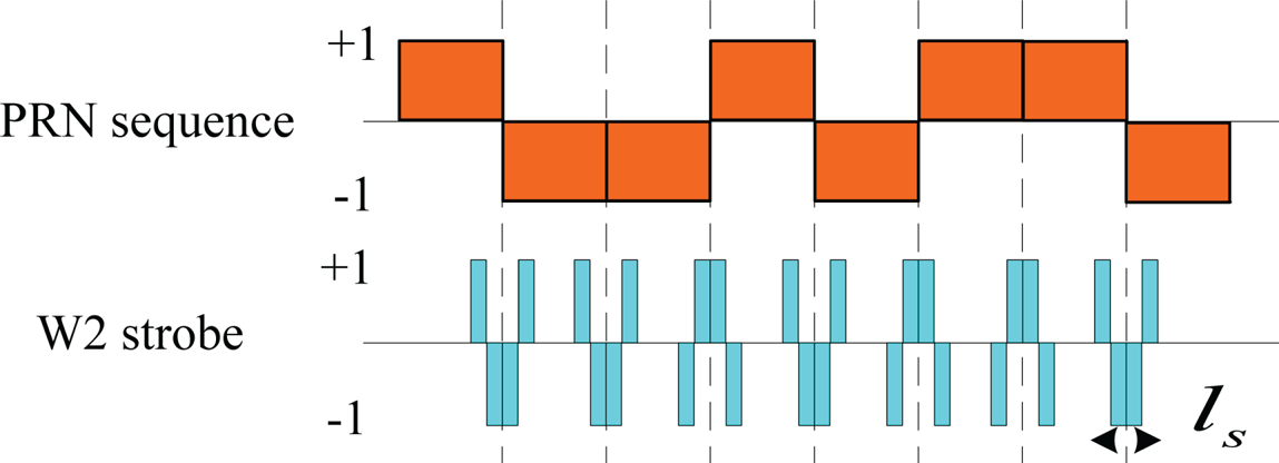
where ε and φ _e are the code and carrier phase estimation bias relative to the received signal, respectively. $N_{\tilde {X}X} =N_{I_{\tilde {X}X} } +jN_{Q_{\tilde {X}X} } $ defines the complex Gaussian noise after the coherent integration operation with a period of T. The band-limited auto-correlation function (ACF) $R_{\tilde {X}X} ( \varepsilon ) $ is determined according to the signal structure and is affected by the front-end bandwidth. The infinite bandwidth ACFs corresponding to the BPSK(1), BOC(1,1) and MBOC(6,1,4/33) signals are reported in Figure 1, in which it can be seen that BOC and MBOC obtain additional zero-crossings, leading to the potential for ambiguous code discrimination. Fortunately, this problem has been discussed and solved in several studies (Lohan et al., Reference Lohan, Diego, Lopez-Salcedo, Seco-Granados, Boto and Fernandes2017; Xiong et al., Reference Xiong, Wang, Gong, Peng, Shi and Tang2018), and the original early-minus-late (EML) processing is not recommended for a robust tracking for BOC modulation. In the pursuit of an anti-multipath tracking, the strobe technique should also prevent unambiguous problems, especially when applied to the new GNSS modulation. The strobe pulse-like sequence is generated by referring to the PRN code sequence. The W2-shape strobe pattern, demonstrated in Figure 2, was proposed for a GPS L1 C/A signal (Veitsel et al., Reference Veitsel, Zhdanov and Zhodzishsky1998) with a well-symmetry and a significant anti-multipath performance. The strobe pulse occurs at each transition of the PRN chip, and the sign of the current generated strobe pulse is determined by the next chip.

Figure 1.

ACF for different civil GNSS signals under infinite bandwidth conditions.

Figure 2.

W2 strobe sequence for BPSK modulation.

The strobe sequence is employed in the incoming signal processing with IQ demodulation and coherent integration, which is given by a complex form as

(3)$$\begin{align} U_{\tilde {X}W} (\varepsilon) &= I_{\tilde {X}W} (\varepsilon )+jQ_{\tilde {X}W} (\varepsilon )\nonumber \\ & = \frac{1}{T}\left\{ {\int_0^T {\sqrt {2C} \tilde {X}(t-{\mathop{\tau} \limits^{\frown}}_0 )W(t-{\tau }_0 )} +\tilde {n}(t)W(t-{\mathop{\tau} \limits^{\frown}}_0 )dt} \right\}\exp (j\varphi _e )\nonumber \\ & = \sqrt {2C} R_{\tilde {X}W} (\varepsilon )\exp (\varphi _e )+N_{\tilde {X}W} \end{align}$$

where W(t) is the strobe sequence. The band-limited CCF denoted as $R_{\tilde {X}W} ( \varepsilon$) is supposed to provide a discrimination shape-like function without an EML operation. It can be seen from Figure 3 that the W2 strobe correlation can satisfy this requirement. However, there is still some undesired part at the +1 chip bias waiting for post-processing. The non-coherent strobe is thus proposed via dot-product type processing as follows:

Figure 3.

W2 strobe correlation function for BPSK(1) modulation.

(4)$$\begin{align} D(\varepsilon) &= I_{\tilde {X}X} (\varepsilon )I_{\tilde {X}W} (\varepsilon )+Q_{\tilde {X}X} (\varepsilon )Q_{\tilde {X}W} (\varepsilon )\nonumber\\ &= 2CR_{{\rm dot}} (\varepsilon )+N_{W2} \end{align}$$

where $R_{{\rm dot}} ( \varepsilon ) =R_{\tilde {X}X} ( \varepsilon) R_{\tilde {X}W} ( \varepsilon$) plotted in Figure 3 defines the non-coherent strobe correlation function with the noise term N _W2, which accounts for the sum of the three terms:

(5)$$\begin{align} N_{W2} &= \sqrt {2C} ( {R_{\tilde {X}X} (\varepsilon )N_{I_{\tilde {X}W} } +R_{\tilde {X}W} (\varepsilon )N_{I_{\tilde {X}X} } } ) \cos (\varphi _e )\nonumber \\ &\quad+ \sqrt {2C} ( {R_{\tilde {X}X} (\varepsilon )N_{Q_{\tilde {X}W} } +R_{\tilde {X}W} (\varepsilon )N_{Q_{\tilde {X}X} } } ) \sin (\varphi _e ) \end{align}$$

As for the BOC modulation, the above strobe scheme is not suitable, as the BOC correlation function is entirely different from that of the BPSK. Additional strobe patterns have been designed for modernised modulations, whereas the W2 strobe can still be used for BOC(1,1)-based navigation signal discrimination with some modification. The W2 discrimination function should ensure that there is no false lock region on the discrimination function sharing the same pull-in order with the correct pull-in range. In this paper, the most straightforward W2-PRN strobe correlator is selected for the BOC(1,1) and MBOC(6,1,4/33) modulations. The dot-product process is implemented with the BOC-PRN correlation function, where BOC-PRN represents the CCF between the BOC(1,1) signal with its PRN code sequence without a sub-carrier. The BOC-PRN is defined as:

(6)$$\begin{align} U_{\tilde {X}C} (\varepsilon) &= I_{\tilde {X}C} (\varepsilon )+jQ_{\tilde {X}C} (\varepsilon )\nonumber \\ & = \frac{1}{T}\left\{ {\int_0^T {\sqrt {2C} \tilde {X}(t-\tau_0 )c(t-{\mathop{\tau} \limits^{\frown}}_0 )} +\tilde {n}(t)c(t-{\mathop{\tau} \limits^{\frown}}_0 )dt} \right\}\exp (j\varphi _e ) \nonumber\\ & = \sqrt {2C} R_{\tilde {X}C} (\varepsilon )\exp (\varphi _e )+N_{\tilde {X}C} \end{align}$$

As indicated in (Wu and Dempster, Reference Wu and Dempster2009), the BOC-PRN curve can be used as a rough BOC signal discrimination function. However, the shifted BOC-PRN correlation function is multiplied with W2-BOC(1,1) CCF to remove the ambiguous region. The non-coherent equation is obtained with

(7)$$d(\varepsilon )=I_{\tilde {X}C} \left( {\varepsilon +\frac{T_c }{2}} \right)I_{\tilde {X}W} (\varepsilon )+Q_{\tilde {X}C} \left( {\varepsilon +\frac{T_c }{2}} \right)Q_{\tilde {X}W} (\varepsilon )$$

where T _c defines the code period of the PRN sequence. This equation is also applicable for the MBOC signal, with the BOC(1,1) case demonstrated in Figure 4. The ambiguous zero-crossing at the +1 code delay vanishes after the BOC-PRN multiplication, thus the W2 strobe correlation is modified to generate an unambiguous discrimination function.

Figure 4.

W2 strobe correlation for BOC(1,1) modulation and the unambiguous modification with the BOC-PRN correlation.

By using the strobe correlation function as the discrimination function, the pull-in range can be changeable with different strobe widths. The compromise between anti-multipath performance and noise resistance prevents the strobe pulse being too narrow. Thus the short-delay multipath correlation can still pollute the line of sight (LOS) correlation, which is able to cause a meter-level ranging error for the receiver (Wu and Dempster, Reference Wu and Dempster2012a).

3. MEDLL

The key concept in the MEDLL is to estimate simultaneously the delay and phase of all of the received signals, including the LOS and multipath components, thus the multipath rays coming with the LOS signal can be separated via the MEDLL technique. The filtered signal accounting for m multipath components is defined as

(8)$$\begin{align} \tilde {s}_m (t) &= \sqrt {2C} \tilde {X}(t-\tau _0 )\exp \{ {j(\omega_0 t+\varphi_0 )} \} \nonumber \\ &\quad + \sum_{i=1}^m {\sqrt {2C} \alpha _i \tilde {X}(t-\tau _0 -\tau _i )\exp \{ {j(\omega_0 t+\varphi_0 +\varphi_i )} \} } +\tilde {n}(t) \end{align}$$

where α _i, τ _i and φ _i(i = 1, …, m) define the multipath attenuation, code phase delay and carrier phase delay relative to the LOS signal corresponding to each multipath ray. The output at the end of the coherent integration process is given by Yang et al. (Reference Yang, Qin and Yuan2017):

(9)$$\begin{align} U_{\tilde {X}X}^m (\varepsilon)&= I_{\tilde {X}X}^m (\varepsilon )+jQ_{\tilde {X}X}^m (\varepsilon ) \nonumber\\ & = C\left\{ {R_{\tilde {X}X} (\varepsilon )\exp \{ {j\varphi_e } \} +\sum_{i=1}^m {\alpha_i R_{\tilde {X}X} (\varepsilon -\tau_i )\exp \{ {j(\varphi_e +\varphi_i )} \} } } \right\}+N_{\tilde {X}X} \end{align}$$

Abundant correlators are required for reconstructing the CCF between the local replica and the received GNSS signal. Next, the multipath correlations superposed on the LOS correlation can be distinguished according to the ML principle. The correlators are usually uniformly deployed within the pull-in range of the discrimination function to avoid omitting every possible multipath component that introduces error into the tracking loop. Here, the correlator number is set to 2M + 1, and the sampling value of the multipath correlation function at each correlator is given by

(10)$$\begin{align} U_{\tilde {X}X}^m (\varepsilon +\delta _k ) &= I_{\tilde {X}X}^m (\varepsilon +\delta _k )+jQ_{\tilde {X}X}^m (\varepsilon +\delta _k )\nonumber \\ & = C\left\{ {R_{\tilde {X}X} (\varepsilon +\delta_k )\exp \{ {j\varphi_e } \} +\sum_{i=1}^m {\alpha_i R_{\tilde {X}X} (\varepsilon +\delta_k -\tau_i )\exp \{ {j(\varphi_e +\varphi_i )} \} } } \right\}+N_{\tilde {X}X}^k \nonumber\\ k &= -M,-M+1,\cdots M-1,M \end{align}$$

where δ _k = kΔ defines the position of each correlator, where Δ = δ _k+1 − δ _k is the spacing between two neighbouring correlators. The MEDLL calculates the estimation principle that minimises

(11)$$L_i ({\mathop{a} \limits^{\frown}} _i, {\mathop{\tau} \limits^{\frown}} _i, {\mathop{\varphi} \limits^{\frown}} _i )=\int_0^T {\left\| {s_m (t)-q_m (t)} \right\|} ^2dt$$

where q _m (t) denotes the estimate of the LOS plus the multipath signals with the estimates of different parameters, including the code phase delay ${\mathop{\tau} \limits^{\frown}} _{i} $, the carrier phase delay ${\mathop{\varphi} \limits^{\frown}} _{i} $ and the attenuation ${\mathop{\alpha} \limits^{\frown}} _{i} $. Considering a severe multipath interference case with m = 7 multipath rays together with the LOS signal, the multipath parameters with respect to each multipath ray are listed in Table 1. The CCF corresponding to the received signal, the LOS ray and each multipath ray are plotted in Figures 5–6. Only the BPSK(1) case is demonstrated here, and it can be seen that only the last multipath ray, namely, ‘Multipath-7’ with the multipath delay +1·2 chip, does not contribute to the discrimination error, whereas the multipath rays with multipath delay within one chip bias have the potential to cause an additional bias for the correct zero-crossing. It should be indicated that the above analysis assumes no front-end filtering and ‘Multipath-7’ would also affect the LOS correlation if the front-end bandwidth were limited. As indicated in Blanco-Delgado and Nunes (Reference Blanco-Delgado and Nunes2012), the accuracy that can be achieved by the estimation algorithm is upper bounded to a half spacing between correlators, Δ/2. The hardware consumption and computational load can be higher if the desired accuracy rises, as more correlators are needed with an unchangeable estimation region.

Figure 5.

In-phase multipath CCF between the local replica and the multipath polluted incoming signal.

Figure 6.

Out-of-phase multipath CCF between the local replica and the multipath polluted incoming signal.

Table 1.

Multipath parameters.

4. MEDLL ON-STROBE CORRELATION

In this section we introduce our algorithm, which combines the strobe technique with the MEDLL technique to achieve a new anti-multipath algorithm, which is presented with the BPSK(1) signal. If the noise term is omitted, the W2 strobe discrimination function with m multipath components before the dot product can be written as

(12)$$\begin{align} U_{\tilde {X}W}^m (\varepsilon )&= I_{\tilde {X}W}^m (\varepsilon )+jQ_{\tilde {X}W}^m (\varepsilon ) \nonumber\\ & = C\left\{R_{\tilde{X}W}(\varepsilon )\exp \{ {\,j\varphi_e } \} +\sum_{i=1}^m {\alpha_i R_{\tilde {X}W} (\varepsilon -\tau_i )\exp \{ {\,j(\varphi_e +\varphi_i )} \} } \right\}+N_{\tilde {X}W} \end{align}$$

Let α ₀ = 1, τ ₀ = 1, φ ₀ = 1 represent the parameters of the LOS signal, where the noise term is dropped in this section. This equation can be re-written as:

(13)$$U_{\tilde {X}W}^m (\varepsilon )=C\left\{ {\sum_{i=0}^m {\alpha _i R_{\tilde {X}W}(\varepsilon -\tau _i )\exp \left\{ {\,j(\varphi _e +\varphi _i )}\right\}} } \right\}$$

Again, the seven-multipath case is considered for the proposed algorithm. The W2 coherent result is demonstrated in Figures 7 and 8 for the I and Q branches, respectively. The strobe width is set to l _s = T _c/2 here with only the first two multipath strobe correlation functions able to distort the zero-crossing of the LOS strobe discrimination function, which causes the correct zero-crossing to deviate to the right side, relative to the correct position. The advantages of the strobe correlation are obvious compared with the ordinary BPSK(1) CCF shown in Figures 5 and 6; specifically, a narrow strobe discrimination function is less sensitive for the medium- and long-delay multipath components. Thus, we have

Figure 7.

In-phase multipath CCF between the W2 strobe and the multipath polluted incoming signal.

Figure 8.

Out-of-phase multipath CCF between the W2 strobe and the multipath polluted incoming signal.

(14)$$\begin{align} U_{\tilde {X}W}^m (\varepsilon )&=U_{\tilde {X}W}^n (\varepsilon ),-\frac{l_s }{2}< \varepsilon \le \varepsilon _0, {\rm with}: \nonumber \\ U_{\tilde {X}W}^n (\varepsilon )&=C\left\{ {\sum_{i=0}^n {\alpha_i R_{\tilde {X}W}(\varepsilon -\tau_i )\exp \{ {j(\varphi_e +\varphi_i )} \} } } \right\},{\mathop{\tau} \limits^{\frown}} _n < \frac{l_s }{2},{\mathop{\tau} \limits^{\frown}} _{n+1} \ge \frac{l_s }{2} \end{align}$$

where $U_{\tilde {X}W}^{n} ( \varepsilon ) $ defines the polluted strobe correlation functions with only the multipath rays, where the code phase delay is shorter than half of the strobe width, and ε ₀ defines the zero-crossing of the polluted strobe discrimination function. To exceed the limitation of the strobe algorithm, the MEDLL mechanism is used to separate the remaining multipath components from the strobe correlation function by minimising the goal function (Townsend et al., Reference Townsend, Fenton, Van Dierendonck and Van Nee1995; Irsigler et al., Reference Irsigler, Avila-Rodriguez and Hein2005):

(15)$$L_i ({\mathop{a} \limits^{\frown}} _i, {\mathop{\tau} \limits^{\frown}} _i, {\mathop{\varphi} \limits^{\frown}} _i )=\int_{-\frac{l_s }{2}}^{\varepsilon _0 } {\left\| {s_m (t)-q_n (t)} \right\|} ^2dt$$

The ML principle for this equation is achieved with the following three derivatives to zero:

(16)$$\frac{\partial L_i {\mathop{a} \limits^{\frown}}_i, {\mathop{\tau} \limits^{\frown}} _i, {\mathop{\varphi} \limits^{\frown}} _i )}{\partial {\mathop{a} \limits^{\frown}} _i }=0,\quad\frac{\partial L_i ({\mathop{a} \limits^{\frown}} _i, {\mathop{\tau} \limits^{\frown}}_i, {\mathop{\varphi} \limits^{\frown}} _i )}{\partial {\mathop{\tau} \limits^{\frown}} _i }=0 \quad {\rm and} \quad \frac{\partial L_i ({\mathop{a} \limits^{\frown}} _i, {\mathop{\tau} \limits^{\frown}}_i,{\mathop{\varphi} \limits^{\frown}} _i )}{\partial {\mathop{\varphi} \limits^{\frown}} _i }=0$$

In the general case of estimating each multipath ray, the code phase delay estimations for the i − th(0 < i ≤ n) multipath ray are given by maximising the discrimination function residue:

(17)$${\mathop{\tau} \limits^{\frown}} _i =\max \left\{ {\rm Re}\left[U_{\tilde {X}W}^m (\varepsilon )-\sum_{\substack{ k=0 \\ k \not= i }}^n {{\mathop{a} \limits^{\frown}}_k R_{\tilde {X}W} (\varepsilon -{\mathop{\tau} \limits^{\frown}}_k )} \exp (j{\mathop{\varphi} \limits^{\frown}}_i ) \right] \right\},-\frac{l_s }{2}< \varepsilon \le \varepsilon _0$$

Next, the attenuation estimation is achieved by taking the real part of the residue as

(18)$${\mathop{a} \limits^{\frown}} _i ={\rm Re}\left\{ {\left[ {U_{\tilde {X}W}^m (\varepsilon )-\sum_{\substack{ k=0 \\ k\,{\not=}\, i \\ }}^n {{\mathop{a} \limits^{\frown}}_k R_{\tilde {X}W} (\varepsilon -{\mathop{\tau} \limits^{\frown}}_k )} \exp (j{\mathop{\varphi} \limits^{\frown}}_i )} \right]\exp (j{\mathop{\varphi} \limits^{\frown}}_i )} \right\},-\frac{l_s }{2}< \varepsilon \le \varepsilon _0$$

Finally, the carrier phase delay is computed via the complex angle operation as

(19)$${\mathop{\varphi} \limits^{\frown}} _i =\arg \left\{ {U_{\tilde {X}W}^m (\varepsilon )-\sum_{\substack{ k=0 \\ k\,{\not=}\, i }}^n {{\mathop{a} \limits^{\frown}}_k R_{\tilde {X}W} (\varepsilon -{\mathop{\tau} \limits^{\frown}}_k )} \exp (j{\mathop{\varphi} \limits^{\frown}}_k )} \right\},-\frac{l_s }{2}< \varepsilon \le \varepsilon _0$$

As illustrated in Figure 9, two regions, including ε ∈ ( − (l _s/2), ε ₀] and ε ∈ (ε ₀, (l _s/2) − ε ₀], should be covered with correlators to achieve the multipath estimation. The first region, denoted as region-1, is of high priority, which begins from the left end of the discrimination function to the first zero-crossing of the curve. The length of the entire estimation region is set to l _s, thus region-2 is the remaining part to the right of region-1. The estimation principle defined in Equation (15) must hold for region-1, whereas it is not a strict restrictive condition for region-2, that is,

Figure 9.

Deployment of correlators for the multipath estimation algorithm.

(20)$$\begin{cases} {\min \{ {L_i ({\mathop{a} \limits^{\frown}}_i,{\mathop{\tau} \limits^{\frown}}_i, {\mathop{\varphi} \limits^{\frown}}_i )} \}, \varepsilon _0 <\varepsilon \le \displaystyle\frac{l_s}{2}-\varepsilon _0, } \\ {{\rm s.t}:\min \{ {L_i({\mathop{a} \limits^{\frown}}_i,{\mathop{\tau} \limits^{\frown}}_i, {\mathop{\varphi} \limits^{\frown}}_i )} \}, -\displaystyle\frac{l_s }{2}<\varepsilon \le \varepsilon _0 }\end{cases}$$

Assuming C = 1 for simplicity, the estimation procedures are summarised as follows:

Step 1. Determine the estimation regions. The strobe discrimination function $U_{\tilde {X}W}^{m} ( \varepsilon ) $ defined in Equation (13) is calculated with the incoming signal, and the zero-crossing ε ₀ is found to divide the discrimination function into region-1 ε ∈ ( − (l _s/2), ε ₀] and region-2 ε ∈ (ε ₀, (l _s/2) − ε ₀].

Step 2. Estimate the LOS signal. The parameters ${\mathop{\tau} \limits^{\frown}}_{0}, \; {\mathop{a} \limits^{\frown}} _{0} $ and ${\mathop{\varphi} \limits^{\frown}} _{0} $ are computed sequentially. The LOS delay ${\mathop{\tau} \limits^{\frown}}_{0} $ is first estimated in region-1, which should satisfy the condition

(21)$${\rm Re}\{ {U_{\tilde {X}W}^m (\varepsilon -{\mathop{\tau} \limits^{\frown}}_0 +\Delta \varepsilon )} \} ={\rm Re}\{ {U_{\tilde {X}W}^m (\varepsilon -{\mathop{\tau} \limits^{\frown}}_0 -\Delta \varepsilon )} \}, -\frac{l_s }{2}< \varepsilon \le \varepsilon _0$$

Next, ${\mathop{a} \limits^{\frown}}_{0} $ is estimated by referring to the standard discrimination function with the multipath strobe discrimination function according to Equation (18), and ${\mathop{\varphi} \limits^{\frown}} _{0} $ is calculated by comparing the energy on the two branches via a complex angle operation according to Equation (19).

Step 3. Compute the residue for multipath estimation. The calculated LOS parameters, including ${\mathop{\tau} \limits^{\frown}}_{0}, \; {\mathop{a} \limits^{\frown}}_{0} $ and ${\mathop{\varphi} \limits^{\frown}} _{0} $, are used to re-construct the LOS correlation estimation, which is subtracted from the CCF to obtain the residue:

(22)$${\rm Res}(\varepsilon )=U_{\tilde {X}W}^m (\varepsilon)-{\mathop{\alpha} \limits^{\frown}} _0 R_{\tilde {X}W} (\varepsilon-{\mathop{\tau} \limits^{\frown}}_0 )\exp \{ {j{\mathop{\varphi} \limits^{\frown}}_0 } \}$$

Step 4. Estimate the first multipath ray: The first multipath ray can be estimated from the multipath strobe discrimination function residue Res(ε), ${\mathop{\tau} \limits^{\frown}}_{1}, \; {\mathop{a} \limits^{\frown}}_{1} $ and ${\mathop{\varphi} \limits^{\frown}} _{1} $ are calculated as optimum values, as in Step 2. Search ${\mathop{\tau} \limits^{\frown}}_{1} $ in region-1 first:

(23)$${\rm Re}\{ {{\rm Res}(\varepsilon -{\mathop{\tau} \limits^{\frown}}_1 +\Delta \varepsilon )} \} ={\rm Re}\{ {{\rm Res}(\varepsilon -{\mathop{\tau} \limits^{\frown}}_1 -\Delta \varepsilon )} \}, -\frac{l_s }{2}< \varepsilon \le \varepsilon _0$$

If this condition cannot be satisfied in region-1, expand the search region into region-2:

(24)$${\rm Re}\{ {{\rm Res}(\varepsilon -{\mathop{\tau} \limits^{\frown}}_1 +\Delta \varepsilon )} \} ={\rm Re}\{ {{\rm Res}(\varepsilon -{\mathop{\tau} \limits^{\frown}}_1 -\Delta \varepsilon )} \}, -\frac{l_s }{2}< \varepsilon \le \frac{l_s }{2}-\varepsilon _0$$

If this condition still cannot be satisfied in this region, go to Step 8.

Step 5. Compute the residue discrimination function for re-estimation of the LOS signal. The multipath correlation is reconstructed with ${\mathop{\tau} \limits^{\frown}} _{1}, \; {\mathop{a} \limits^{\frown}} _{1} $ and ${\mathop{\varphi} \limits^{\frown}} _{1} $ and is employed to obtain the residue for LOS re-estimation:

(25)$${\rm Res}(\varepsilon )=U_{\tilde {X}W}^m (\varepsilon )-{\mathop{\alpha} \limits^{\frown}} _1 R_{W2} (\varepsilon -{\mathop{\tau} \limits^{\frown}}_1 )\exp (j{\mathop{\varphi} \limits^{\frown}} _1 )$$

Step 6. Re-estimate the LOS signal. ${\mathop{\tau} \limits^{\frown}}_{0}, \; {\mathop{a} \limits^{\frown}}_{0} $ and ${\mathop{\varphi} \limits^{\frown}}_{0}$ are re-calculated according to the procedures described in Step 2.

Step 7. Estimate the remaining multipath ray by iteration: The remaining multipath components are estimated by repeating Step 3 to Step 6. Once the stop criterion is fulfilled, go to Step 8. The stop criterion in this paper is defined as

(26)$$\begin{align} L_i ({\mathop{a} \limits^{\frown}} _i, {\mathop{\tau} \limits^{\frown}}_i, {\mathop{\varphi} \limits^{\frown}} _i )&= \frac{1}{\varepsilon _0 +(l_s /2)}\int_{-(l_s /2)}^{\varepsilon _0 } {\vert {U_{\tilde {X}W}^m (\varepsilon )-{\mathop{U} \limits^{\frown}}_{\tilde {X}W}^n (\varepsilon )} \vert } d\varepsilon \nonumber\\ & = \frac{1}{\varepsilon _0 +(l_s /2)}\int_{-(l_s /2)}^{\varepsilon _0 } {\left| {U_{\tilde {X}W}^m (\varepsilon )-\sum_{i=0}^n {{\mathop{\alpha} \limits^{\frown}}_i R_{W2} (\varepsilon -{\mathop{\tau} \limits^{\frown}}_i )\exp (j{\mathop{\varphi} \limits^{\frown}}_i )} } \right|} d\varepsilon \nonumber \\ &< \beta \frac{{\mathop{C} \limits^{\frown}} \times {\mathop{a} \limits^{\frown}} _0 }{C/N_0 }\approx \beta {\mathop{N} \limits^{\frown}} _0 \end{align}$$

where V(ε) defines the estimation residue of region-1, and defines a constant value with respect to the threshold, which can be set according to the practical situation.

Step 8. Declare that the multipath estimation is finished.

The LOS signal is re-estimated continuously once a new multipath is determined to exist. Thus, the estimation accuracy can be improved steadily through this iteration, the diagram of which is illustrated in Figure 10. The relationship between the number of multipath rays and of estimation procedures is given by

Figure 10.

Multipath estimation procedures based on the W2 strobe correlation.

(27)$$n_{{\rm MEDLL}} =\begin{cases} 3 & {n=1} \\ {\displaystyle\sum_{i=5}^{n+3} i +3} & {n\ge 2} \end{cases}$$

This indicates that the operational complexity of the MEDLL increases as the multipath rays increase, and it could become remarkably high when n becomes a large figure. Thus the ordinary MEDLL technique based on the standard ACF could be time-consuming and of high operational complexity once the multipath pollution is severe. On the contrary, the proposed signal processing structure is able to eliminate the medium- and long-delay multipath interference before the short-delay multipath rays are estimated with the MEDLL algorithm. Therefore, the operational burden can be alleviated significantly.

The estimation result is demonstrated in Figure 11. 2M + 1 = 401 correlators are therefore used, and the up-bounded estimation accuracy is given by Δ/2 = 0 · 000625 chip. The reconstructed curve coincides well with the strobe correlation in region-1, though there are still obvious differences compared with the region to the left of region-1. The LOS estimation has finalised as the zero-crossing has been corrected, even though there are still five components that have not been estimated. The residue for the LOS component is given by

Figure 11.

Estimation results for LOS and the first two multipath components.

(28)$${U}'_{\tilde {X}W} (\varepsilon )=U_{\tilde {X}W}^m (\varepsilon)-\sum_{i=1}^n{{\mathop{\alpha} \limits^{\frown}}_i R_{W2} (\varepsilon-{\mathop{\tau} \limits^{\frown}}_i )\exp(j{\mathop{\varphi} \limits^{\frown}} _i )}$$

Finally, the dot-product combination is used to eliminate the potential ambiguity before the discrimination result is sent to the loop filter, which is given by

(29)$${D}'(\varepsilon )=I_{\tilde {X}X} (\varepsilon ){I}'_{\tilde {X}W} (\varepsilon )+Q_{\tilde {X}X} (\varepsilon ){Q}'_{\tilde {X}W} (\varepsilon )$$

where ${I}'_{\tilde {X}W} ( \varepsilon ) $ and ${Q}'_{\tilde {X}W} ( \varepsilon ) $ define the in-phase and out-of-phase branches of ${U}'_{\tilde {X}W} ( \varepsilon ) $, respectively. The final result is demonstrated in Figure 12.

Figure 12.

Non-coherent combination based on the strobe residue.

5. ANTI-MULTIPATH PERFORMANCE ANALYSIS

The anti-multipath performance is tested with simulator data to verify the advantages of the proposed method. A narrow (0·2 chip EML spacing) correlator, a W2 strobe (0·4 chip pulse width) correlator and a corresponding MEDLL are subjected to the same situation. One multipath with a 3 dB attenuation is mixed with the LOS component, and the multipath delay increases from zero sequentially. The LOS zero-crossing would be affected by the multipath correlation; thus an additional bias is produced for the code tracking. The tracking bias under a multipath condition is calculated to evaluate the anti-multipath performance with respect to a certain technique. Multipath error envelope (Irsigler et al., Reference Irsigler, Avila-Rodriguez and Hein2005; Xu et al., Reference Xu, Liu, Tang and Wang2016) is widely used to assess anti-multipath performance, which is given by

(30)$$\tau _1 =\left[ {\mathop {\max }\limits_{\varphi_1 } \gamma (\alpha_1, \tau_1, \varphi_1 ),\mathop {\min }\limits_{\varphi_1 } \gamma (\alpha_1, \tau_1, \varphi_1 )} \right]$$

where γ defines the multipath error introduced by only one multipath ray. The multipath attenuation is usually set to 3 dB with φ ₁ = 0 and φ ₁ = π corresponding to the maximum and minimum values of the multipath error, respectively. The cut off frequencies of the front-end bandwidth are set to 8 MHz, 14 MHz and 20 MHz for the BPSK(1), BOC(1,1) and MBOC(6,1,4/33) cases, respectively, to ensure sufficiently high frequency components are being processed with the correlators, which prevents rounding of the correlation peak and the high-mixed effect between the multipath correlation and the LOS correlation. The correlator numbers employed for the ordinary MEDLL algorithm are set to 101, whereas this number is 26 for the proposed combining algorithm. Thus, the estimation accuracy is up-bounded by Δ/2 = 0 · 0025 chip (0·73 m). The C/N ₀ is set to 45dB-Hz in this experiment, with the results reported in Figures 13–15, respectively.

Figure 13.

BPSK(1) multipath error versus the relative multipath delay for a narrow correlator and strobe correlator and the corresponding MEDLL results.

Figure 14.

BOC(1,1) multipath error versus the relative multipath delay for a narrow correlator and strobe correlator and the corresponding MEDLL results.

Figure 15.

MBOC(6,1,4/33) multipath error versus the relative multipath delay for a narrow correlator and strobe correlator and the corresponding MEDLL results.

It can be seen that the multipath error cannot be eliminated thoroughly. However, the proposed algorithm obtains the best anti-multipath performance among these options, followed by the strobe correlator and ordinary MEDLL. The length of the non-zero error region is significantly reduced to the strobe pattern width, whereas this figure still exceeds one chip for the narrow correlator and ordinary MEDLL techniques. The strobe width is a compromise between the anti-multipath capability and the computational burden of the proposed method with the code tracking accuracy, which should be well considered for the proposed method. A short multipath with code delay τ ₁ = 0 · 013, a ₁ = 3 dB and a random carrier phase delay is added into the LOS signal, which lies between two correlators. Thus the MEDLL is not able to find the accurate multipath delay. The coherent integration period is set to 10 ms and 1,000 runs are conducted for the BPSK(1), BOC(1,1) and MBOC(6,1,4/33) signals. The LOS estimations at under 30 dB-Hz and 40 dB-Hz are reported in Figures 16 and 17, respectively. It can be seen that the multipath estimation is affected by noise, and the 0·0025~; 0·02 chip estimation error still exists under the 30 dB-Hz condition. The BOC(1,1) signal obtains the best LOS estimation accuracy due to its W2 discrimination function. In all, an advanced multipath estimation based on a strobe correlator is achieved to provide a better tracking result.

Figure 16.

Averaged LOS estimation result with 1,000 runs under 30 dB-Hz with a 10 ms coherent integration condition.

Figure 17.

Averaged LOS estimation result with 1,000 runs under 40 dB-Hz with a 10 ms coherent integration condition.

6. ANTI-NOISE PERFORMANCE ANALYSIS

The BPSK signal tracking error for the strobe technique under noise interference can be expressed as by Wu and Dempster (2012):

(31)$$\sigma _{\mbox{BPSK}}^2 \approx \frac{2B_L T\sigma _N^2 }{g_0^2 }=\frac{B_L R_{WW} (0)}{[ ({\rm d}R_{{{\mathop{X} \limits^{\frown}}}W} (\varepsilon ))/({\rm d}\varepsilon ) \vert_{\varepsilon =0} ] ^2 C/N_0} \left[1+\frac{1}{R_{X{{\mathop{X} \limits^{\frown}}}}(0)C/N_0T} \right]$$

where B _L defines the code tracking loop bandwidth, $\sigma_{N}^{2} $ defines the normalised steady-state code tracking error variance and g ₀ defines the discrimination gain. The BOC(1,1) and MBOC(6,1,4/33) cases can be approximated in a similar way:

(32)$$\sigma _{{\rm BOC/MBOC}}^2 \approx \frac{2B_L T\sigma _N^2 }{g_0^2}=\frac{B_L [ {{R_{{\mathop{X} \limits^{\frown}} C}}^2 (\displaystyle\tfrac{T_c}{2})R_{CC} (0)TC} / N_0 +R_{CC}(0)R_{WW} (0) ] }{T[ {C/ N_0 R_{{\mathop{X} \limits^{\frown}}C} (\displaystyle\tfrac{T_c} {2}) {(({\rm d}R_{{\mathop{X} \limits^{\frown}}W} (\varepsilon ))/({\rm d}\varepsilon ))} \vert_{\varepsilon =0} } ] ^2}$$

The code loop bandwidth is set to 1 Hz and the coherent integration is set to 1 ms, where the steady-state tracking error for the BPSK(1), BOC(1,1) and MBOC(6,1,4/33) modulated signals are demonstrated in Figures 18–20, respectively, and compared with the theoretical results. The computer simulation was run 500 times, calculating the average steady-state tracking error for each case. The EML space for the narrow correlator is set to 1/4 chip only and the theoretical results with respect to the narrow correlator can be found in Betz and Kolodziejski (Reference Betz and Kolodziejski2009). The strobe technique shares a similar tracking performance with the proposed method with the same strobe width, where the steady-state tracking accuracy increases as the strobe width narrows down. However, the strobe width should not be set to the smallest possible size, as a narrow discrimination function may lead to a greater possibility of losing lock.

Figure 18.

Steady-state tracking error for the BPSK(1) modulation.

Figure 19.

Steady-state tracking error for the BOC(1,1) modulation.

Figure 20.

Steady-state tracking error for the MBOC(6,1,4/33) modulation.

7. OPERATIONAL COMPLEXITY ANALYSIS

In this section, the proposed method is compared with the MEDLL for operational complexity, with only the BPSK(1) case simulated here. The difference between the ordinary MEDLL technology and the proposed method lies in the complexity of multipath estimation. The average running time for the multipath estimation process is considered here. The correlator number is set to 401 for the original MEDLL algorithm, and 26, 51 and 101 for the l _s = (1/8), l _s = (1/4) and l _s = (1/2) chip, respectively. Thus, the expected multipath estimation accuracies are equivalent for both algorithms. The multipath number is simulated to be a random figure from 1~; r. The code attenuation, code delay and carrier phase delay are also generated randomly for each multipath ray. These figures are all uniformly distributed. Denoting ρ as the operational complexity for one MEDLL procedure demonstrated in Figure 21, the expected value of the original MEDLL operational complexity can be expressed as

Figure 21.

Average running time of estimation procedure.

(33)$$P_{{\rm MEDLL}} =\frac{1}{r}\left[ {3+\sum_{n=2}^r {\left( {\sum_{i=5}^{n+3} {i+3} } \right)} } \right]\rho$$

As indicated in the above section, the strobe discrimination function reduces the range of the estimation domain, thus the operational complexity corresponding to a certain strobe width can be expressed as

(34)$$P_{{\rm Strobe+MEDLL}} =\frac{1}{r'}\left[ {3+\sum_{n=2}^{r'} {\left( {\sum_{i=5}^{n+3} {i+3} } \right)} } \right]\rho, r'=\frac{l_s }{2}r$$

Letting r sweep from 4 to 20, the average running time for 500 simulations is computed and plotted in Figure 21, where C/N ₀ is set to 40 dB-Hz. The theoretical results expressed by Equations (33) and (34) are also demonstrated in this figure, where ρ is determined by the hardware structure and software circumstances, which can be estimated easily. It can be seen the operational complexity can be unacceptable for ordinary MEDLL when r > 12, which would lead to a long running time, causing the tracking loop to fail at updating in time. This problem is solved well with the proposed method, as the average running time increases slowly in this process. Thus, the advantages of the MEDLL on-strobe correlation are verified, both in operational complexity and hardware consumption.