1 Introduction
Granular chute flow is widely encountered in the natural environment (rock avalanches, landslides) as well as in innumerable applications such as the transportation of mineral ores or the handling of grains and powders (Jaeger, Nagel & Behringer Reference Jaeger, Nagel and Behringer1996; Duran Reference Duran2000; Pudasaini & Hutter Reference Pudasaini and Hutter2007; Andreotti, Forterre & Pouliquen Reference Andreotti, Forterre and Pouliquen2013, see chap. 6 in particular; Takahashi Reference Takahashi2014; Köhler et al. Reference Köhler, McElwaine, Sovilla, Ash and Brennan2016). This type of flow is well described by the Saint-Venant equations traditionally used for shallow water, provided that these equations are appropriately modified to account for the special characteristics of granular matter (Savage & Hutter Reference Savage and Hutter1989; Forterre Reference Forterre2006; Gray & Edwards Reference Gray and Edwards2014; Viroulet et al. Reference Viroulet, Baker, Edwards, Johnson, Gjaltema, Clavel and Gray2017). In recent years it has become clear, from a series of experimental and theoretical studies, that granular chute flows exhibit various distinct types of standing and travelling waveforms (Gray, Tai & Noelle Reference Gray, Tai and Noelle2003; Boudet et al. Reference Boudet, Amarouchene, Bonnier and Kellay2007; Johnson & Gray Reference Johnson and Gray2011; Saingier, Deboeuf & Lagrée Reference Saingier, Deboeuf and Lagrée2016; Edwards et al. Reference Edwards, Viroulet, Kokelaar and Gray2017; Mejean, Faug & Einav Reference Mejean, Faug and Einav2017). Which waveform prevails depends largely on the values of the Froude number attained along the chute:
 $$\begin{eqnarray}Fr(x,t)=\frac{\bar{u}(x,t)}{\sqrt{h(x,t)g\cos \unicode[STIX]{x1D701}}}.\end{eqnarray}$$
Here
 $\bar{u}(x,t)$
stands for the depth-averaged velocity of the granular sheet,
 $h(x,t)$
denotes its height,
 $g$
is the gravitational acceleration and
 $\unicode[STIX]{x1D701}$
is the inclination angle of the chute.
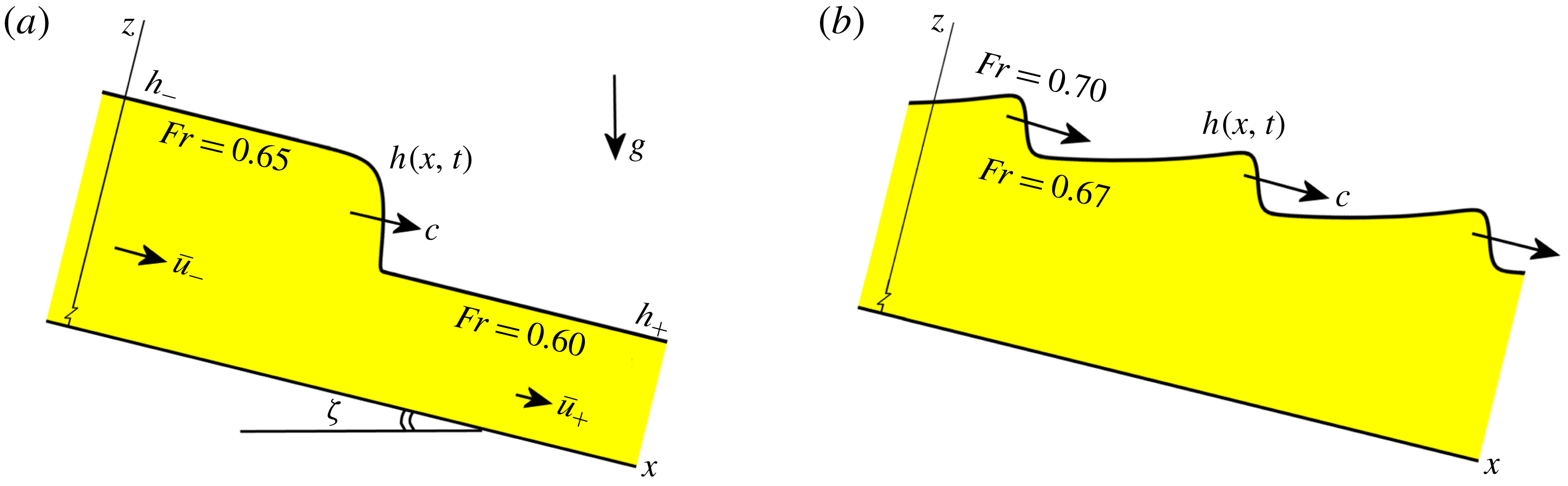
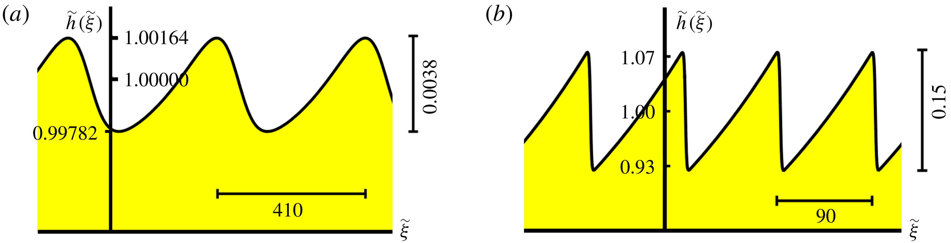
In figure 1 we show two of the main waveforms: (i) the granular monoclinal wave and (ii) a train of roll waves. The former may be generated when a granular reservoir at the top of the chute, first opened only partially such as to produce a thin sheet of height
 $h_{+}$
, is subsequently opened further to permit a sheet of greater height
 $h_{-}$
. The monoclinal wave is stable for
 $Fr<2/3$
(Razis, Kanellopoulos & van der Weele Reference Razis, Kanellopoulos and van der Weele2018) whereas roll waves are found for
 $Fr>2/3$
(Gray & Edwards Reference Gray and Edwards2014; Razis et al.
Reference Razis, Edwards, Gray and van der Weele2014; Edwards & Gray Reference Edwards and Gray2015). In the present paper we focus upon the transition between these two waveforms at the critical Froude number
 $Fr=2/3$
. We do this by studying the dynamical system that governs the travelling wave solutions of the Saint-Venant equations, following the series of events taking place in the phase plane from the demise of the monoclinal wave to the emergence of stable roll waves.
(a) Granular monoclinal flood wave on a chute (Razis et al.
Reference Razis, Kanellopoulos and van der Weele2018): a surge of uniform height
 $h_{-}$
and depth-averaged velocity
 $\bar{u}_{-}$
overtakes a shallower and slower flow of height
 $h_{+}$
and velocity
 $\bar{u}_{+}$
. The monoclinal wave, being the travelling shock structure connecting these two regions, is stable for Froude numbers
 $Fr_{+}<Fr_{-}<2/3$
. It propagates at a wave speed
 $c$
exceeding the velocities of both plateaus, i.e.
 $c>\bar{u}_{-}>\bar{u}_{+}$
. (b) A train of granular roll waves (Gray & Edwards Reference Gray and Edwards2014; Razis et al.
Reference Razis, Edwards, Gray and van der Weele2014; Edwards & Gray Reference Edwards and Gray2015): for
 $Fr_{-}>2/3$
the high plateau of the monoclinal wave becomes unstable owing to the granular Kapitza instability and spontaneously breaks into a series of roll waves. The shock front of the monoclinal wave provides the required height perturbation for the instability to manifest itself. A similar fate befalls a flowing sheet of uniform thickness (which may be thought of as a degenerate monoclinal wave with
 $h_{-}=h_{+}$
) when its Froude number exceeds the critical value of
 $2/3$
. In the latter case, the roll waves are generated by small random fluctuations in the height of the sheet. In both panels, the inclination of the chute has been explicitly depicted; throughout the rest of the paper the
 $x$
-axis will be drawn horizontally, with the understanding that the chute is in fact tilted by an angle
 $\unicode[STIX]{x1D701}$
.

The two waveforms mentioned above are not restricted to granular flows but have their counterparts also in normal fluids. In fact, they are two of the most widely studied travelling wave solutions of the Saint-Venant equations for shallow water flow. Especially the study of roll waves has a long tradition in fluid mechanics (Dressler Reference Dressler1949; Needham & Merkin Reference Needham and Merkin1984; Balmforth & Mandre Reference Balmforth and Mandre2004; Fowler Reference Fowler2011) but also monoclinal flood waves are well documented (Moots & Mavis Reference Moots and Mavis1938; Whitham Reference Whitham1974; Le Méhauté Reference Le Méhauté1976; Ferrick Reference Ferrick2005; Shome & Steffler Reference Shome and Steffler2006; Fowler Reference Fowler2011).
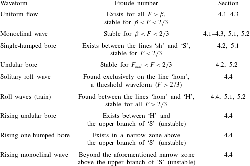
The paper is organized as follows. In § 2 we give the governing equations, being the one-dimensional Saint-Venant equations adapted to the granular context, with custom-made constitutive relations for the friction with the chute and the in-plane stresses within the sheet, i.e. the normal stresses on the plane perpendicular to the flow. Also in § 2 we give a brief review of the aforementioned monoclinal and roll wave solutions of the Saint-Venant equations. In § 3 we derive the dynamical system that governs all possible travelling wave solutions. We locate the fixed points of this dynamical system (each of which turns out to correspond to uniform flow conditions, i.e. flat regions of constant thickness and velocity) and determine their local stability properties as a function of the control parameters. In § 4 we supplement this information with the phase-plane portraits to arrive at a global view of the dynamics. This enables us to identify not only the monoclinal wave of figure 1(a) (which in the phase plane is represented by a heteroclinic connection between two fixed points) and the roll wave of figure 1(b) (which takes the form of a limit cycle), but also a series of other travelling-wave solutions that correspond to intermediate stages in the transition between these two waveforms. Among these is a novel undular variant of the granular monoclinal wave, which to the best of our knowledge has never before been reported in the literature; we call it the undular bore. In § 5 we present the sequence of events as a function of increasing Froude number of the incoming flow. This is arguably the most accessible path through the space of control parameters from an experimental point of view. Along this path one encounters all the waveforms, starting from a stable monoclinal wave and ending with a train of stable roll waves. Finally, in § 6 we recapitulate our results and make concluding remarks.
2 The governing equations
2.1 The Saint-Venant equations for granular chute flow
In the spirit of the one-dimensional Saint-Venant approach for shallow water, granular chute flow can be described in terms of the height of the granular sheet,
 $h(x,t)$
, and the depth-averaged velocity,
 $\bar{u}(x,t)$
. In this description, the detailed velocity profile
 $u(x,z,t)$
is replaced by its average:
 $$\begin{eqnarray}\bar{u}(x,t)=\frac{1}{h(x,t)}\int _{0}^{h(x,t)}u(x,z,t)\,\text{d}z,\end{eqnarray}$$
whereas any variations in the cross-wise direction (
 $y$
) are ignored. Hence both the height of the sheet
 $h(x,t)$
and its velocity
 $\bar{u}(x,t)$
are taken to depend only on
 $x$
and
 $t$
(cf. figure 1). We will further assume that the granular sheet has a constant density, which means that it will be treated as an incompressible fluid.
The two quantities
 $h(x,t)$
and
 $\bar{u}(x,t)$
are governed by a system of two nonlinear differential equations (Gray & Edwards Reference Gray and Edwards2014; Razis et al.
Reference Razis, Edwards, Gray and van der Weele2014; Edwards & Gray Reference Edwards and Gray2015; Razis et al.
Reference Razis, Kanellopoulos and van der Weele2018), namely the mass conservation
 $$\begin{eqnarray}\frac{\unicode[STIX]{x2202}h}{\unicode[STIX]{x2202}t}+\frac{\unicode[STIX]{x2202}}{\unicode[STIX]{x2202}x}(h\bar{u})=0\end{eqnarray}$$
and the momentum balance
 $$\begin{eqnarray}\frac{\unicode[STIX]{x2202}}{\unicode[STIX]{x2202}t}(h\bar{u})+\frac{\unicode[STIX]{x2202}}{\unicode[STIX]{x2202}x}(h\bar{u}^{2})=gh\sin \unicode[STIX]{x1D701}-\frac{\unicode[STIX]{x2202}}{\unicode[STIX]{x2202}x}\left(\frac{1}{2}gh^{2}\cos \unicode[STIX]{x1D701}\right)-\unicode[STIX]{x1D707}(h,\bar{u})gh\cos \unicode[STIX]{x1D701}+\frac{\unicode[STIX]{x2202}}{\unicode[STIX]{x2202}x}\left(\unicode[STIX]{x1D708}h^{3/2}\frac{\unicode[STIX]{x2202}\bar{u}}{\unicode[STIX]{x2202}x}\right).\end{eqnarray}$$
The four terms on the right-hand side of this momentum balance represent (i) the component of gravity working in the
 $x$
-direction, with
 $g=9.81~\text{m}~\text{s}^{-2}$
as usual; (ii) the downstream force arising from variations in
 $h(x,t)$
, i.e. the negative gradient of the depth-averaged lithostatic pressure
 $(1/2)gh^{2}\cos \unicode[STIX]{x1D701}$
within the sheet; (iii) the frictional force exerted by the chute, which is modelled as a (height- and velocity-dependent) friction coefficient
 $\unicode[STIX]{x1D707}(h,\bar{u})$
multiplied by the normal reaction force acting on the granular sheet (Pouliquen Reference Pouliquen1999; Razis et al.
Reference Razis, Edwards, Gray and van der Weele2014); and (iv) the viscous-like diffusive term
 $\unicode[STIX]{x2202}_{x}(\unicode[STIX]{x1D708}h^{3/2}\unicode[STIX]{x2202}_{x}\bar{u})$
arising from depth-averaging the in-plane stresses in the sheet (Gray & Edwards Reference Gray and Edwards2014). This is the granular analogue of the term
 $\unicode[STIX]{x1D708}\unicode[STIX]{x2202}_{xx}\bar{u}$
introduced by Needham & Merkin (Reference Needham and Merkin1984) for water, which proved to be an essential extension of the shallow water equations, allowing them to obtain continuous roll wave solutions. Indeed, the diffusive term only comes into action when there are variations in
 $\bar{u}(x,t)$
(implying also variations in
 $h(x,t)$
) and its main role is to smooth out such variations.
Due to the very gentle slopes of the granular waveforms we will encounter, the viscous term in (2.3) always remains several orders of magnitude smaller than any of the other contributing forces, even at the shock fronts (Razis et al. Reference Razis, Kanellopoulos and van der Weele2018). Nevertheless, also in the granular context it is a crucial ingredient of the momentum balance in order to guarantee that the solutions obtained will be free of discontinuities.
For completeness, we note that the advective term
 $\unicode[STIX]{x2202}_{x}(h\bar{u}^{2})$
in (2.3) may be multiplied by a shape factor to obtain an optimal correspondence with experiments (Saingier et al.
Reference Saingier, Deboeuf and Lagrée2016; Lagrée et al.
Reference Lagrée, Saingier, Deboeuf, Staron, Popinet, Radjai, Nezamadi, Luding and Delenne2017). This factor, also known as the Boussinesq parameter, depends on the exact form of the velocity profile
 $u(x,z,t)$
. For plug flow it is equal to unity, and this is the choice we adopt here. Other values used in the literature (all close to
 $1$
) may be anticipated to yield qualitatively similar results.
The above equations (2.2) and (2.3) must be supplemented by constitutive relations for the pressure, the basal friction and the viscous-like term. For the pressure we assume that it grows linearly with depth, which is a good approximation as long as the granular sheet is sufficiently shallow and saturation effects may be ignored (Duran Reference Duran2000; Gray & Edwards Reference Gray and Edwards2014). This assumption underlies the form of the second term on the right-hand side of (2.3).
For the friction coefficient various expressions have been proposed in the literature (Savage & Hutter Reference Savage and Hutter1989; Daerr & Douady Reference Daerr and Douady1999; Pouliquen & Forterre Reference Pouliquen and Forterre2002). Here we adopt the expression first introduced by Pouliquen (Reference Pouliquen1999) and presented in the following form by Razis et al. (Reference Razis, Edwards, Gray and van der Weele2014), which gives an accurate description as long as the granular material is fully dynamic and does not exhibit stopping regions (Pouliquen & Forterre Reference Pouliquen and Forterre2002; Edwards & Gray Reference Edwards and Gray2015):
 $$\begin{eqnarray}\unicode[STIX]{x1D707}(h,\bar{u})=\tan \unicode[STIX]{x1D701}_{1}+\frac{\tan \unicode[STIX]{x1D701}_{2}-\tan \unicode[STIX]{x1D701}_{1}}{1+\unicode[STIX]{x1D6FD}{\mathcal{L}}^{-1}\sqrt{g\cos \unicode[STIX]{x1D701}}h^{3/2}\bar{u}^{-1}},\end{eqnarray}$$
where
 $\unicode[STIX]{x1D701}_{1}$
,
 $\unicode[STIX]{x1D701}_{2}$
,
 ${\mathcal{L}}$
and
 $\unicode[STIX]{x1D6FD}$
are experimental parameters. The angles
 $\unicode[STIX]{x1D701}_{1}$
and
 $\unicode[STIX]{x1D701}_{2}$
denote the two inclination angles that delimit the interval in which uniform granular flows are possible. For
 $\unicode[STIX]{x1D701}<\unicode[STIX]{x1D701}_{1}$
the granular sheet remains at rest, whereas for
 $\unicode[STIX]{x1D701}>\unicode[STIX]{x1D701}_{2}$
it sweeps downwards in an accelerated fashion. For definiteness we take
 $\unicode[STIX]{x1D701}_{1}=32.9^{\circ }$
and
 $\unicode[STIX]{x1D701}_{2}=42.0^{\circ }$
, which are the same experimental values used in two previous studies of ours (Razis et al.
Reference Razis, Edwards, Gray and van der Weele2014, Reference Razis, Kanellopoulos and van der Weele2018), while the inclination angle of the chute is for the moment chosen to be
 $\unicode[STIX]{x1D701}=33.3^{\circ }$
. The influence of varying the angle
 $\unicode[STIX]{x1D701}$
will be discussed later.
The parameter
 ${\mathcal{L}}$
in the above friction law is an empirical length scale, namely the deposition thickness. It is determined through independent experiments in which one terminates the inflow at the top of the chute and measures the height of the deposited layer after the flow has come to a halt. Its value depends on the specifics of the particles and the chute; typically it is of the order of 1–2 particle diameters. We will use the value
 ${\mathcal{L}}=1~\text{mm}$
, which corresponds to granular particles with a diameter of approximately 0.7 mm on a laboratory chute. For geophysical flows (rock avalanches on mountainsides, debris flows, etc.) the value of
 ${\mathcal{L}}$
will scale up accordingly.
Given
 ${\mathcal{L}}$
, the dimensionless fit parameter
 $\unicode[STIX]{x1D6FD}$
is determined by measuring the depth-averaged velocity of a uniformly flowing granular sheet as a function of its thickness, and then fitting the data with (2.6) below. So
 $\unicode[STIX]{x1D6FD}$
and
 ${\mathcal{L}}$
are related. Realistic values found in the literature include
 $\unicode[STIX]{x1D6FD}=0.136$
and
 ${\mathcal{L}}=0.65~\text{mm}$
for smooth glass beads (Pouliquen & Forterre Reference Pouliquen and Forterre2002),
 $\unicode[STIX]{x1D6FD}=0.65$
and
 ${\mathcal{L}}=1~\text{mm}$
for rough carborundum particles (Razis et al.
Reference Razis, Edwards, Gray and van der Weele2014; Edwards & Gray Reference Edwards and Gray2015) and
 $\unicode[STIX]{x1D6FD}=0.63$
and
 ${\mathcal{L}}=0.44~\text{mm}$
again for carborundum particles (Gray & Edwards Reference Gray and Edwards2014; Edwards et al.
Reference Edwards, Viroulet, Kokelaar and Gray2017). We choose
 $\unicode[STIX]{x1D6FD}=0.5$
and
 ${\mathcal{L}}=1~\text{mm}$
as typical values; one of the reasons for this choice is to make the present study directly comparable to a previous paper on the granular monoclinal wave, where the same values for
 $\unicode[STIX]{x1D6FD}$
and
 ${\mathcal{L}}$
were used (Razis et al.
Reference Razis, Kanellopoulos and van der Weele2018). The physical interpretation of
 $\unicode[STIX]{x1D6FD}$
is that it sets the threshold for the Froude number below which the granular sheet ceases to be fully dynamic. That is to say, for
 $Fr\leqslant \unicode[STIX]{x1D6FD}$
the sheet develops ‘stopping regions’ where the frictional force outweighs gravity, causing the sheet to be locally decelerated until it comes to a standstill (Edwards & Gray Reference Edwards and Gray2015). One then needs the extended form of Pouliquen’s friction law (Pouliquen & Forterre Reference Pouliquen and Forterre2002) but this is not required in the present study, since we focus upon fully dynamic granular flows with
 $Fr>\unicode[STIX]{x1D6FD}$
everywhere.
Finally, with respect to the constitutive relation for the effective viscosity,
 $\unicode[STIX]{x2202}_{x}(\unicode[STIX]{x1D708}h^{3/2}\unicode[STIX]{x2202}_{x}\bar{u})$
, we note that a term of this form had originally been introduced on physical grounds by Forterre in Reference Forterre2006. For the precise coefficient
 $\unicode[STIX]{x1D708}$
we adopt the analytical expression derived by Gray & Edwards (Reference Gray and Edwards2014):
 $$\begin{eqnarray}\unicode[STIX]{x1D708}=\unicode[STIX]{x1D708}(\unicode[STIX]{x1D701})=\frac{2{\mathcal{L}}\sqrt{g}\sin \unicode[STIX]{x1D701}}{9\unicode[STIX]{x1D6FD}\sqrt{\cos \unicode[STIX]{x1D701}}}\unicode[STIX]{x1D6FE}(\unicode[STIX]{x1D701}),\quad \text{where }\unicode[STIX]{x1D6FE}(\unicode[STIX]{x1D701})=\frac{\tan \unicode[STIX]{x1D701}_{2}-\tan \unicode[STIX]{x1D701}}{\tan \unicode[STIX]{x1D701}-\tan \unicode[STIX]{x1D701}_{1}}.\end{eqnarray}$$
Apart from the fact that this expression for
 $\unicode[STIX]{x1D708}(\unicode[STIX]{x1D701})$
has been derived from first principles, it has the added advantage that it does not diverge for
 $h\rightarrow 0$
as was the case for the term proposed by Forterre. For the parameter values chosen in the present study (with
 ${\mathcal{L}}$
,
 $\unicode[STIX]{x1D6FD}$
,
 $\unicode[STIX]{x1D701}_{1}$
and
 $\unicode[STIX]{x1D701}_{2}$
as introduced above and
 $g=9.81~\text{m}~\text{s}^{-2}$
) we get
 $\unicode[STIX]{x1D708}(\unicode[STIX]{x1D701})=0.0014\unicode[STIX]{x1D6FE}(\unicode[STIX]{x1D701})\sin \unicode[STIX]{x1D701}/\sqrt{\cos \unicode[STIX]{x1D701}}$
. For the specific choice
 $\unicode[STIX]{x1D701}=33.3^{\circ }$
one has
 $\unicode[STIX]{x1D6FE}(\unicode[STIX]{x1D701})=24.48$
, giving the value
 $\unicode[STIX]{x1D708}=0.0205~\text{m}^{3/2}~\text{s}^{-1}$
.
We note that the expression for
 $\unicode[STIX]{x1D708}(\unicode[STIX]{x1D701})$
given in (2.5) is tailor-made for our purposes, since its domain of validity coincides exactly with the range
 $\unicode[STIX]{x1D701}_{1}<\unicode[STIX]{x1D701}<\unicode[STIX]{x1D701}_{2}$
where steady granular flows are possible. Outside this interval, equation (2.5) gives non-physical negative values for
 $\unicode[STIX]{x1D708}(\unicode[STIX]{x1D701})$
; this can be traced back to the fact that the Bagnold velocity profile on which its derivation is based – and the underlying balance between gravity and friction – breaks down for these values of
 $\unicode[STIX]{x1D701}$
(GDR-MiDi, 2004; Gray & Edwards Reference Gray and Edwards2014; Barker et al.
Reference Barker, Schaeffer, Bohorquez and Gray2015). In the relevant range
 $\unicode[STIX]{x1D701}_{1}<\unicode[STIX]{x1D701}<\unicode[STIX]{x1D701}_{2}$
the coefficient
 $\unicode[STIX]{x1D708}(\unicode[STIX]{x1D701})$
is a monotonically decreasing function of
 $\unicode[STIX]{x1D701}$
, from infinity at
 $\unicode[STIX]{x1D701}=\unicode[STIX]{x1D701}_{1}$
(reflecting the fact that the sheet is still stagnant at this limiting angle) to zero at
 $\unicode[STIX]{x1D701}=\unicode[STIX]{x1D701}_{2}$
(heralding the regime of accelerated flows).
2.2 Three basic solutions of the granular Saint-Venant equations
The most elementary solution of the granular Saint-Venant equations (2.2)–(2.3) is that of steady uniform flow, i.e. when the sheet has a uniform thickness
 $h_{0}$
and flows at constant velocity
 $\bar{u}_{0}$
. In this case, all derivatives with respect to
 $x$
and
 $t$
vanish, so (2.2) is satisfied trivially. In (2.3) the only terms that survive are those of gravity and friction, which must therefore precisely balance each other:
 $\tan \unicode[STIX]{x1D701}=\unicode[STIX]{x1D707}(h,\bar{u})$
. This yields, with the friction law (2.4), the following relation between the velocity and the thickness of the uniformly flowing sheet, being the depth-averaged Bagnold velocity profile (Bagnold Reference Bagnold1966; Duran Reference Duran2000):
 $$\begin{eqnarray}\bar{u}_{0}=\frac{\unicode[STIX]{x1D6FD}\sqrt{g\cos \unicode[STIX]{x1D701}}}{{\mathcal{L}}\unicode[STIX]{x1D6FE}(\unicode[STIX]{x1D701})}h_{0}^{3/2}.\end{eqnarray}$$
The corresponding Froude number measured in the laboratory frame is
 $$\begin{eqnarray}Fr=Fr(h_{0},\bar{u}_{0})=\frac{\bar{u}_{0}}{\sqrt{gh_{0}\cos \unicode[STIX]{x1D701}}}=\frac{\unicode[STIX]{x1D6FD}}{{\mathcal{L}}\unicode[STIX]{x1D6FE}(\unicode[STIX]{x1D701})}h_{0},\end{eqnarray}$$
which is a linearly increasing function of the sheet thickness. The uniform flow is stable for
 $Fr<2/3$
and turns unstable beyond this value via the granular counterpart of the Kapitza instability (Kapitza & Kapitza Reference Kapitza and Kapitza1949; Forterre & Pouliquen Reference Forterre and Pouliquen2003; Gray & Edwards Reference Gray and Edwards2014). The Kapitza instability in thin films of a normal fluid is responsible for the formation of capillary ripples. In the case of dry granular matter, where surface tension is absent, the analogous instability does not give rise to capillary waves but rather to a series of roll waves (Forterre Reference Forterre2006).
The second basic solution we should mention here is the monoclinal wave, which consists of two uniformly moving plateaus linked together via a shock front (Razis et al.
Reference Razis, Kanellopoulos and van der Weele2018), as depicted in figure 1(a). The upstream plateau (with relatively large thickness
 $h_{-}$
and velocity
 $\bar{u}_{-}$
) has a higher Froude number than the downstream plateau (with smaller
 $h_{+}$
and
 $\bar{u}_{+}$
). The speed of the shock front is given by the well-known formula (Whitham Reference Whitham1974)
 $$\begin{eqnarray}c=\frac{h_{-}\bar{u}_{-}-h_{+}\bar{u}_{+}}{h_{-}-h_{+}},\end{eqnarray}$$
which can be inferred directly from the fact that, for an observer in the co-moving frame, the flux of material entering the shock structure must be equal to the flux leaving the shock, i.e.
 $h_{+}(\bar{u}_{+}-c)=h_{-}(\bar{u}_{-}-c)$
. We note that the shock speed (2.8) exceeds the velocities of both plateaus:
 $c>\bar{u}_{-}>\bar{u}_{+}$
. The monoclinal wave is stable for
 $Fr(h_{-},\bar{u}_{-})<2/3$
, which automatically guarantees that
 $Fr(h,\bar{u})$
is below the critical value
 $2/3$
along the entire span of the wave. Simultaneously, in the present study we require that
 $Fr(h_{+},\bar{u}_{+})>\unicode[STIX]{x1D6FD}$
in order to ensure that the monoclinal wave is fully dynamic everywhere.
Using the fact that the plateaus of the monoclinal wave are two regions of uniform flow, meaning that the velocities
 $\bar{u}_{\pm }$
are related to the corresponding heights
 $h_{\pm }$
via (2.6), the above expression (2.8) for the shock speed can be cast in the following form:
 $$\begin{eqnarray}c=\frac{\unicode[STIX]{x1D6FD}\sqrt{g\cos \unicode[STIX]{x1D701}}}{{\mathcal{L}}\unicode[STIX]{x1D6FE}(\unicode[STIX]{x1D701})}\left(\frac{h_{-}^{5/2}-h_{+}^{5/2}}{h_{-}-h_{+}}\right).\end{eqnarray}$$
This relation for the wave speed no longer contains the velocities
 $\bar{u}_{\pm }$
but is fully expressed in terms of the heights alone.
A third important solution of the granular Saint-Venant equations is the roll wave (figure 1 b), which usually comes in the form of a periodic wave train. Each member of the wave train consists of a long exponentially rising flank, gradually building up to a peak, followed by a steep descent (a shock front) linking the peak to the shallower downstream flow; and from this level the wave starts to rise again. The speed of the roll wave is
 $$\begin{eqnarray}c=\frac{h_{b}\bar{u}_{b}-h_{a}\bar{u}_{a}}{h_{b}-h_{a}},\end{eqnarray}$$
where the subscripts
 $b$
and
 $a$
stand for ‘before’ and ‘after’ the shock, respectively. That is, the height
 $h_{b}$
corresponds to the crest of the roll wave, whereas
 $h_{a}$
denotes the smaller height immediately after the sudden drop in height. Evidently, equation (2.10) is of the same general form as the wave speed (2.8) for the monoclinal wave, and it follows from the same conservation principle in the co-moving frame. In the case of roll waves, however, the peak height
 $h_{b}$
is not equal to the thickness of the incoming flow; it is in fact larger than that. Another difference is that (2.10) cannot be augmented by the uniform flow condition (2.6) since the roll waves do not exhibit any regions that are truly flat.
Roll waves are known to appear in granular chute flow when
 $Fr>2/3$
. They are born either from small height perturbations to the uniform flow (which is unstable at these Froude numbers), as has been shown by Gray & Edwards (Reference Gray and Edwards2014), or from the destabilization of the monoclinal wave as we will demonstrate in this paper. In the latter scenario, no height perturbations are needed, since the shock front of the monoclinal wave serves as such. Indeed, it is exactly here (at the upper side of the shock front) that the roll waves are born when we let
 $Fr(h_{-},\bar{u}_{-})$
grow beyond
 $2/3$
. A preview of the early stages of this transition from a monoclinal profile to a roll wave structure was presented by Razis et al. (Reference Razis, Kanellopoulos and van der Weele2018). Here we will provide the complete story.
3 A dynamical systems approach to travelling waves
3.1 Formulation of the dynamical system governing travelling waveforms
The aforementioned waveforms (i.e. monoclinal waves and roll waves) are structures propagating without change of shape, and at a constant velocity, and therefore constitute travelling wave solutions to (2.2)–(2.3) of the general form
 $$\begin{eqnarray}h(x,t)=h(x-ct)=h(\unicode[STIX]{x1D709})\quad \text{and}\quad \bar{u}(x,t)=\bar{u}(x-ct)=\bar{u}(\unicode[STIX]{x1D709}),\end{eqnarray}$$
where
 $\unicode[STIX]{x1D709}=x-ct$
is the standard variable for a wave travelling to the right with constant speed
 $c$
. Substituting the form (3.1) into the mass balance (2.2) and denoting the differentiation with respect to
 $\unicode[STIX]{x1D709}$
with a prime, we obtain
 $-ch^{\prime }+(h\bar{u})^{\prime }=0$
, which can readily be integrated to give
 $$\begin{eqnarray}-ch+h\bar{u}=-K.\end{eqnarray}$$
The negative integration constant
 $-K=h(\bar{u}-c)$
represents the flux of material measured in the co-moving frame; the fact that this quantity must be constant was already noted earlier in the context of the expression for the shock speed (2.8). We note that
 $\bar{u}-c$
is negative, meaning that the relative motion of the particles observed in the co-moving frame is directed in the negative
 $x$
-direction, i.e. upstream. It is understood that we are talking about the depth-averaged motion of the particles here. That the same statement can apply to even the fastest particles in the flow may be inferred from experiments such as those by Viroulet et al. (Reference Viroulet, Baker, Rocha, Johnson, Kokelaar and Gray2018), who showed (for the case of bidisperse granular roll waves) that the large particles in the fast surface layer were moving slower than the waves.
For the granular monoclinal wave, the constant
 $K$
can be written as follows (taking as reference values those of the incoming flow, i.e.
 $h=h_{-}$
and
 $\bar{u}=\bar{u}_{-}$
):
 $$\begin{eqnarray}K=-h_{-}(\bar{u}_{-}-c)=-\frac{\unicode[STIX]{x1D6FD}\sqrt{g\cos \unicode[STIX]{x1D701}}}{{\mathcal{L}}\unicode[STIX]{x1D6FE}(\unicode[STIX]{x1D701})}h_{-}\left(h_{-}^{3/2}-\frac{h_{-}^{5/2}-h_{+}^{5/2}}{h_{-}-h_{+}}\right),\end{eqnarray}$$
where we have used the form of
 $c$
given in (2.9). Thus, the velocities
 $\bar{u}_{\pm }$
have dropped from the equation and
 $K$
is expressed as a function of the heights
 $h_{\pm }$
only.
As for the momentum balance equation (2.3), we first rewrite the left-hand side, with the aid of the continuity equation (2.2), in the form
 $h(\unicode[STIX]{x2202}_{t}\bar{u}+\bar{u}\unicode[STIX]{x2202}_{x}\bar{u})$
. Then, upon substituting the ansatz (3.1) and dividing throughout by
 $h$
, the momentum balance reads
 $$\begin{eqnarray}-c\bar{u}^{\prime }+\bar{u}\bar{u}^{\prime }=g\sin \unicode[STIX]{x1D701}-g\cos \unicode[STIX]{x1D701}h^{\prime }-\unicode[STIX]{x1D707}(h,\bar{u})g\cos \unicode[STIX]{x1D701}+\unicode[STIX]{x1D708}({\textstyle \frac{3}{2}}h^{-1/2}h^{\prime }\bar{u}^{\prime }+h^{1/2}\bar{u}^{\prime \prime }).\end{eqnarray}$$
The velocity
 $\bar{u}(\unicode[STIX]{x1D709})$
and all its derivatives can be eliminated from this equation using (3.2), or equivalently,
 $\bar{u}=c-Kh^{-1}$
. With
 $\bar{u}^{\prime }=Kh^{-2}h^{\prime }$
and
 $\bar{u}^{\prime \prime }=-2Kh^{-3}(h^{\prime })^{2}+Kh^{-2}h^{\prime \prime }$
, the momentum balance (3.4) then turns into a second-order ordinary differential equation (ODE) for
 $h(\unicode[STIX]{x1D709})$
alone:
 $$\begin{eqnarray}\frac{\unicode[STIX]{x1D708}K}{h^{3/2}}h^{\prime \prime }-\frac{\unicode[STIX]{x1D708}K}{2h^{5/2}}(h^{\prime })^{2}+\left(\frac{K^{2}}{h^{3}}-g\cos \unicode[STIX]{x1D701}\right)h^{\prime }+g\sin \unicode[STIX]{x1D701}-\unicode[STIX]{x1D707}(h)g\cos \unicode[STIX]{x1D701}=0.\end{eqnarray}$$
Because of the substitution
 $\bar{u}=c-Kh^{-1}$
, also the friction coefficient
 $\unicode[STIX]{x1D707}(h,\bar{u})$
has now become a function of
 $h$
alone, i.e.
 $\unicode[STIX]{x1D707}(h)$
. In the same spirit, also the constant
 $K$
has already been expressed in terms of the heights
 $h_{\pm }$
(see (3.3)).
The second-order ODE (3.5) governs all travelling waveforms that are sustained by the Saint-Venant equations (2.2)–(2.3) for granular chute flow. This same equation featured already in a recent paper on the granular monoclinal wave (Razis et al. Reference Razis, Kanellopoulos and van der Weele2018); in the present study we go beyond the monoclinal waveform and explore the full spectrum of its solutions.
At this point, it is convenient to introduce non-dimensional variables (denoted by a tilde) as follows:
 $h=h_{-}\tilde{h}$
and
 $\unicode[STIX]{x1D709}=h_{-}\tilde{\unicode[STIX]{x1D709}}$
. That is, all length scales (in the transversal and longitudinal directions alike) are measured in terms of the thickness
 $h_{-}$
of the incoming flow. With this rescaling, the differential equation (3.5) takes the non-dimensional form
 $$\begin{eqnarray}\frac{\text{d}^{2}\tilde{h}}{\text{d}\tilde{\unicode[STIX]{x1D709}}^{2}}-\frac{1}{2\tilde{h}}\left(\frac{\text{d}\tilde{h}}{\text{d}\tilde{\unicode[STIX]{x1D709}}}\right)^{2}+\frac{R\tilde{h}^{3/2}}{F^{2}(\tilde{c}-1)}\left[\left(\frac{F^{2}(\tilde{c}-1)^{2}}{\tilde{h}^{3}}-1\right)\frac{\text{d}\tilde{h}}{\text{d}\tilde{\unicode[STIX]{x1D709}}}+\tan \unicode[STIX]{x1D701}-\unicode[STIX]{x1D707}(\tilde{h})\right]=0.\end{eqnarray}$$
This equation first appeared in a study by Gray & Edwards (Reference Gray and Edwards2014) on granular roll waves. A similar equation for normal fluids was derived by Needham & Merkin (Reference Needham and Merkin1984) in their pioneering paper on the modelling of roll waves as continuous periodic solutions without the need of piecing together continuous sections by a series of hydraulic jumps.
In (3.6) the non-dimensional friction coefficient
 $\unicode[STIX]{x1D707}(\tilde{h})$
assumes the form
 $$\begin{eqnarray}\unicode[STIX]{x1D707}(\tilde{h})=\tan \unicode[STIX]{x1D701}_{1}+(\tan \unicode[STIX]{x1D701}_{2}-\tan \unicode[STIX]{x1D701}_{1})\frac{1-\tilde{c}+\tilde{c}\tilde{h}}{1-\tilde{c}+\tilde{c}\tilde{h}+\unicode[STIX]{x1D6FE}(\unicode[STIX]{x1D701})\tilde{h}^{5/2}}\end{eqnarray}$$
and the non-dimensional numbers
 $R$
and
 $F$
are given by
 $$\begin{eqnarray}R=\frac{\unicode[STIX]{x1D6FD}\sqrt{g\cos \unicode[STIX]{x1D701}}h_{-}^{2}}{{\mathcal{L}}\unicode[STIX]{x1D6FE}(\unicode[STIX]{x1D701})\unicode[STIX]{x1D708}(\unicode[STIX]{x1D701})}\quad \text{and}\quad F=\frac{\unicode[STIX]{x1D6FD}h_{-}}{{\mathcal{L}}\unicode[STIX]{x1D6FE}(\unicode[STIX]{x1D701})}.\end{eqnarray}$$
The latter two are the Reynolds and Froude numbers of the incoming flow, as noted by Gray & Edwards (Reference Gray and Edwards2014). This can be seen by restoring them to a form which also contains the velocity
 $\bar{u}_{-}=\unicode[STIX]{x1D6FD}({\mathcal{L}}\unicode[STIX]{x1D6FE}(\unicode[STIX]{x1D701}))^{-1}\sqrt{g\cos \unicode[STIX]{x1D701}}h_{-}^{3/2}$
(cf. (2.6)):
 $$\begin{eqnarray}R=\frac{\bar{u}_{-}\sqrt{h_{-}}}{\unicode[STIX]{x1D708}(\unicode[STIX]{x1D701})}\quad \text{and}\quad F=\frac{\bar{u}_{-}}{\sqrt{gh_{-}\cos \unicode[STIX]{x1D701}}}.\end{eqnarray}$$
As far as the Froude number is concerned, one recognizes the familiar definition applicable also to standard fluids. The Reynolds number is slightly different, containing
 $\sqrt{h_{-}}$
rather than
 $h_{-}$
, which is necessary because the granular viscous-like coefficient
 $\unicode[STIX]{x1D708}(\unicode[STIX]{x1D701})$
is measured in
 $\text{m}^{3/2}~\text{s}^{-1}$
, whereas the usual kinematic viscosity is measured in
 $\text{m}^{2}~\text{s}^{-1}$
. We note that this granular Reynolds number
 $R$
is in fact not an independent parameter but, with the use of
 $F$
in (3.8b
) and
 $\unicode[STIX]{x1D708}(\unicode[STIX]{x1D701})$
as in (2.5), can be written as
 $$\begin{eqnarray}R=\frac{9F^{2}}{2\tan \unicode[STIX]{x1D701}}.\end{eqnarray}$$
So the Reynolds number
 $R$
of the incoming flow is fully determined by
 $F$
and
 $\unicode[STIX]{x1D701}$
.
Before we proceed, let us also note that the dimensionless wave speed
 $\tilde{c}$
appearing in (3.6) is not a free parameter but is in fact determined by the heights and velocities characterizing the waveform in question, as indicated by (2.8) and (2.10). In particular, for the monoclinal wave (which is the starting point from which we will explore all the other waveforms) we get
 $$\begin{eqnarray}\tilde{c}=\frac{c}{\bar{u}_{-}}=\frac{1-\tilde{h}_{+}^{5/2}}{1-\tilde{h}_{+}},\end{eqnarray}$$
where for
 $c$
we have used the expression (2.9), while
 $\bar{u}_{-}=\unicode[STIX]{x1D6FD}({\mathcal{L}}\unicode[STIX]{x1D6FE}(\unicode[STIX]{x1D701}))^{-1}\sqrt{g\cos \unicode[STIX]{x1D701}}h_{-}^{3/2}$
as dictated by the uniform flow condition (2.6). The relation (3.11) shows that the non-dimensional shock speed
 $\tilde{c}$
depends solely on the dimensionless height of the downstream plateau
 $\tilde{h}_{+}=h_{+}/h_{-}$
.
Equation (3.6) is the non-dimensional counterpart of (3.5) governing all travelling waveforms. Being a second-order ODE, it can also be written as a system of two first-order ODEs. Taking into account (3.10) to eliminate
 $R$
, we arrive at the following dynamical system:
 $$\begin{eqnarray}\displaystyle & \displaystyle \frac{\text{d}\tilde{h}}{\text{d}\tilde{\unicode[STIX]{x1D709}}}=\tilde{s}=f(\tilde{h},\tilde{s}), & \displaystyle\end{eqnarray}$$
 $$\begin{eqnarray}\displaystyle & \displaystyle \frac{\text{d}\tilde{s}}{\text{d}\tilde{\unicode[STIX]{x1D709}}}=\frac{\tilde{s}^{2}}{2\tilde{h}}-\frac{9\tilde{h}^{3/2}}{2\tan \unicode[STIX]{x1D701}(\tilde{c}-1)}\left[\left(\frac{F^{2}(\tilde{c}-1)^{2}}{\tilde{h}^{3}}-1\right)\tilde{s}+\tan \unicode[STIX]{x1D701}-\unicode[STIX]{x1D707}(\tilde{h})\right]=g(\tilde{h},\tilde{s}),\qquad & \displaystyle\end{eqnarray}$$
 $\tilde{s}$
to represent the slope
 $\text{d}\tilde{h}/\text{d}\tilde{\unicode[STIX]{x1D709}}$
of the non-dimensional height profile
 $\tilde{h}(\tilde{\unicode[STIX]{x1D709}})$
.
We observe that the right-hand side of the first equation of the above system, equation (3.12a
), does not depend on
 $\tilde{h}$
but only on
 $\tilde{s}$
, so
 $f(\tilde{h},\tilde{s})=f(\tilde{s})$
with
 $f(\tilde{s})=\tilde{s}$
. As a result, the fixed points of this dynamical system are always such that
 $\tilde{s}=0$
, corresponding to flat regions of the flow; we will see this in more detail in the next subsection.
3.2 Fixed points and linear stability analysis
The fixed points of the dynamical system (3.12) are found by setting both
 $\text{d}\tilde{h}/\text{d}\tilde{\unicode[STIX]{x1D709}}$
and
 $\text{d}\tilde{s}/\text{d}\tilde{\unicode[STIX]{x1D709}}$
equal to zero, i.e.
 $f(\tilde{s})=0$
and
 $g(\tilde{h},\tilde{s})=0$
. From (3.12a
) it immediately transpires that any fixed point must have
 $\tilde{s}=0$
, meaning that the point lies on the
 $\tilde{h}$
-axis in the
 $(\tilde{h},\tilde{s})$
phase plane. The associated value of
 $\tilde{h}$
is then determined from (3.12b
) with
 $\tilde{s}=0$
, which reduces to
 $$\begin{eqnarray}\unicode[STIX]{x1D707}(\tilde{h})=\tan \unicode[STIX]{x1D701}.\end{eqnarray}$$
In this equation we recognize the well-known balance between friction and gravity characteristic of a uniformly flowing sheet (cf. our discussion of the uniform solution in § 2.2). Its emergence in the context of the fixed points, which represent flat regions of constant thickness, is only natural. This balance of forces (3.13), with the aid of (3.7), translates to
 $$\begin{eqnarray}\tilde{h}^{5/2}=1-\tilde{c}+\tilde{c}\tilde{h}.\end{eqnarray}$$
This equation always admits, for all values of
 $\tilde{c}$
, the evident solution
 $\tilde{h}=\tilde{h}_{-}=1$
(i.e. our reference thickness) corresponding to the flat incoming flow which in the phase plane is represented by the point
 $(\tilde{h},\tilde{s})=(1,0)$
. For
 $\tilde{c}>1$
a second physically meaningful solution (real and positive) comes into existence, which we will call
 $\tilde{h}=\tilde{h}_{+}$
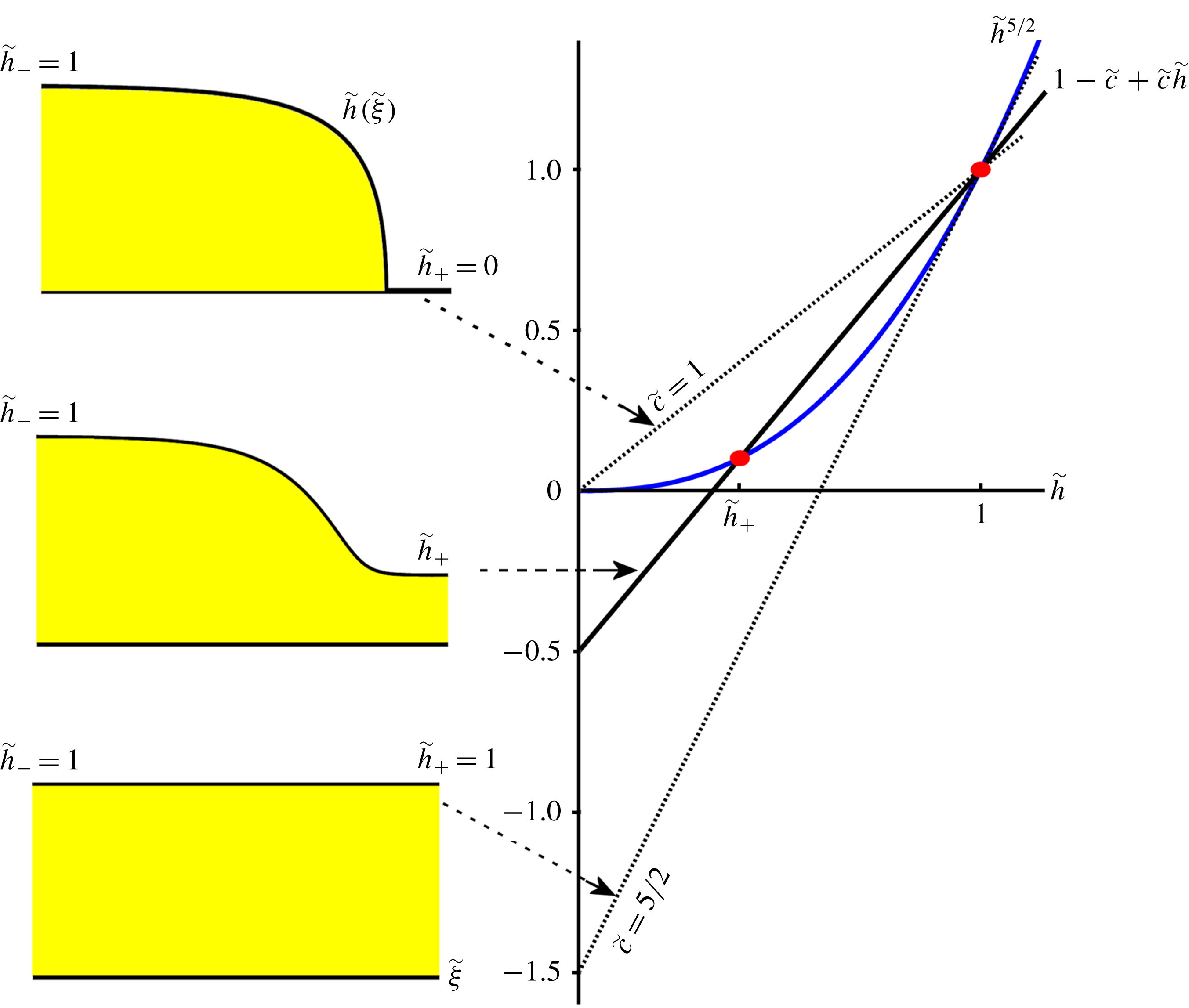
. This is illustrated in figure 2. For the monoclinal waveform this second fixed point
 $(\tilde{h},\tilde{s})=(\tilde{h}_{+},0)$
represents the uniform flow at the downstream end of the chute. Its value rises from
 $\tilde{h}_{+}=0$
at
 $\tilde{c}=1$
to
 $\tilde{h}_{+}=1$
for
 $\tilde{c}=5/2$
. The first case (
 $\tilde{h}_{+}=0$
) corresponds to an avalanche front propagating on an empty chute, at a constant speed
 $\tilde{c}=1$
or equivalently
 $c=\bar{u}_{-}$
. This case actually admits an analytic solution (Gray & Ancey Reference Gray and Ancey2009; Razis et al.
Reference Razis, Kanellopoulos and van der Weele2018), closely related to the classical Bresse solution for gradually varied flow in water channels (Bresse Reference Bresse1860; Rouse & Ince Reference Rouse and Ince1963). The second limiting case (with
 $\tilde{h}_{+}=1$
and
 $\tilde{c}=5/2$
) corresponds to the uniform solution, since here both fixed points coincide at
 $(\tilde{h},\tilde{s})=(1,0)$
; that is, the incoming and outgoing flow now have the same thickness.
For non-dimensional velocities
 $\tilde{c}>5/2$
, the value of
 $\tilde{h}_{+}$
exceeds unity. This however does not introduce new waveforms. Rather,
 $\tilde{h}_{+}$
now plays the role of
 $\tilde{h}_{-}$
and vice versa. In order to see this, let us consider a monoclinal wave. As long as
 $\tilde{h}_{+}$
is less than
 $\tilde{h}_{-}=1$
, this wave is characterized by a high inflow plateau of thickness
 $\tilde{h}_{-}=1$
and a low outflow plateau of thickness
 $\tilde{h}_{+}$
. Its non-dimensional speed
 $\tilde{c}$
is less than
 $5/2$
and given by (3.11), an expression which follows from (3.14) as well.
Now, imagine the same monoclinal waveform but this time normalized with respect to
 $h_{+}$
instead of
 $h_{-}$
. Then the high inflow plateau has non-dimensional thickness
 $h_{-}/h_{+}=1/\tilde{h}_{+}>1$
and the outflow plateau has non-dimensional thickness
 $h_{+}/h_{+}=1$
. In this alternative normalization, the non-dimensional shock speed is given by
 $$\begin{eqnarray}\tilde{c}_{alt}=\frac{(1/\tilde{h}_{+})^{5/2}-1}{(1/\tilde{h}_{+})-1}=\tilde{h}_{+}^{-3/2}\frac{1-\tilde{h}_{+}^{5/2}}{1-\tilde{h}_{+}}=\tilde{h}_{+}^{-3/2}\tilde{c}.\end{eqnarray}$$
The crux of the matter is that this velocity
 $\tilde{c}_{alt}$
is larger than
 $5/2$
.
We conclude that for every waveform with fixed points
 $(\tilde{h}_{+},0)$
and
 $(1,0)$
(with
 $\tilde{h}_{+}<1$
) and non-dimensional speed
 $\tilde{c}<5/2$
, there exists an equivalent dual waveform with the fixed points
 $(1,0)$
and
 $(1/\tilde{h}_{+},0)$
and non-dimensional speed
 $\tilde{h}_{+}^{-3/2}\tilde{c}>5/2$
. These waveforms are the same, the only difference between them being the different choice of normalization. This is the reason why we may restrict our attention to the regime
 $1\leqslant \tilde{c}\leqslant 5/2$
; the regime
 $\tilde{c}>5/2$
does not give rise to any new waveforms.
As a side remark, we recall that in the present study we focus on fully dynamic waveforms without stopping regions. As we have seen in § 2, this means that we require
 $Fr>\unicode[STIX]{x1D6FD}$
everywhere. With
 $Fr(h_{+},\bar{u}_{+})=\unicode[STIX]{x1D6FD}h_{+}/{\mathcal{L}}\unicode[STIX]{x1D6FE}(\unicode[STIX]{x1D701})$
(cf. (2.7)) this yields
 $h_{+}>{\mathcal{L}}\unicode[STIX]{x1D6FE}(\unicode[STIX]{x1D701})=\unicode[STIX]{x1D6FD}h_{-}/F$
, where we have used (3.8). Hence, for fully dynamic waveforms we require
 $\tilde{h}_{+}=h_{+}/h_{-}>\unicode[STIX]{x1D6FD}/F$
, i.e. the lower bound of
 $\tilde{h}_{+}$
then lies above zero. Correspondingly, the lower bound of the dimensionless wave speed lies above
 $1$
and is equal to
 $(1-(\unicode[STIX]{x1D6FD}/F)^{5/2})/(1-(\unicode[STIX]{x1D6FD}/F))$
.
Graphical solution of (3.14), yielding the fixed points of the dynamical system (3.12a–b
). The solution
 $\tilde{h}=1$
, and thereby the fixed point
 $(\tilde{h},\tilde{s})=(1,0)$
, is seen to exist for all values of
 $\tilde{c}$
. The second solution
 $\tilde{h}=\tilde{h}_{+}$
, corresponding to the fixed point
 $(\tilde{h},\tilde{s})=(\tilde{h}_{+},0)$
, is physically meaningful (i.e. real and non-negative) only for
 $\tilde{c}\geqslant 1$
. The value of
 $\tilde{h}_{+}$
increases monotonically with
 $\tilde{c}$
, from
 $\tilde{h}_{+}=0$
at
 $\tilde{c}=1$
to
 $\tilde{h}_{+}=1$
at
 $\tilde{c}=5/2$
. At the latter instant the two fixed points coincide, reducing the monoclinal wave to a uniform flow. For
 $\tilde{c}>5/2$
the value of
 $\tilde{h}_{+}$
exceeds
 $1$
; this does not introduce new waveforms though (as explained in the text) so we restrict ourselves to
 $1\leqslant \tilde{c}\leqslant 5/2$
.

The linear stability properties of these fixed points are determined by the eigenvalues of the Jacobian matrix:
 $$\begin{eqnarray}\unicode[STIX]{x1D645}=\left.\left(\begin{array}{@{}cc@{}}{\displaystyle \frac{\unicode[STIX]{x2202}f}{\unicode[STIX]{x2202}\tilde{h}}} & {\displaystyle \frac{\unicode[STIX]{x2202}f}{\unicode[STIX]{x2202}\tilde{s}}}\\ {\displaystyle \frac{\unicode[STIX]{x2202}g}{\unicode[STIX]{x2202}\tilde{h}}} & {\displaystyle \frac{\unicode[STIX]{x2202}g}{\unicode[STIX]{x2202}\tilde{s}}}\end{array}\right)\right|_{(\tilde{h},\tilde{s})=(\tilde{h}_{\pm },0)}=\left.\left(\begin{array}{@{}cc@{}}0 & 1\\ {\displaystyle \frac{\unicode[STIX]{x2202}g}{\unicode[STIX]{x2202}\tilde{h}}} & {\displaystyle \frac{\unicode[STIX]{x2202}g}{\unicode[STIX]{x2202}\tilde{s}}}\end{array}\right)\right|_{(\tilde{h},\tilde{s})=(\tilde{h}_{\pm },0)},\end{eqnarray}$$
where the functions
 $f=f(\tilde{s})=\tilde{s}$
and
 $g=g(\tilde{h},\tilde{s})$
are given by (3.12a
) and (3.12b
), respectively. So
 $$\begin{eqnarray}\displaystyle & \displaystyle \frac{\unicode[STIX]{x2202}g}{\unicode[STIX]{x2202}\tilde{h}}=\frac{9\unicode[STIX]{x1D6E4}(\unicode[STIX]{x1D701})}{4\tan \unicode[STIX]{x1D701}}\frac{5\tilde{c}-3\tilde{c}\tilde{h}-5}{(\tilde{c}-1)\tilde{h}^{2}}\quad (=-\text{det}\,J), & \displaystyle\end{eqnarray}$$
 $$\begin{eqnarray}\displaystyle & \displaystyle \frac{\unicode[STIX]{x2202}g}{\unicode[STIX]{x2202}\tilde{s}}=\frac{9\tilde{h}^{3/2}(1-F^{2}(\tilde{c}-1)^{2}\tilde{h}^{-3})}{2\tan \unicode[STIX]{x1D701}(\tilde{c}-1)}\quad (=TrJ), & \displaystyle\end{eqnarray}$$
 $$\begin{eqnarray}\unicode[STIX]{x1D6E4}(\unicode[STIX]{x1D701})=\frac{(\tan \unicode[STIX]{x1D701}_{2}-\tan \unicode[STIX]{x1D701}_{1})\unicode[STIX]{x1D6FE}(\unicode[STIX]{x1D701})}{(1+\unicode[STIX]{x1D6FE}(\unicode[STIX]{x1D701}))^{2}}.\end{eqnarray}$$
The eigenvalues of the matrix
 $\unicode[STIX]{x1D645}$
are the solutions of the quadratic equation
 $\unicode[STIX]{x1D706}^{2}-(\unicode[STIX]{x2202}g/\unicode[STIX]{x2202}\tilde{s})\unicode[STIX]{x1D706}-(\unicode[STIX]{x2202}g/\unicode[STIX]{x2202}\tilde{h})=0$
, i.e.
 $$\begin{eqnarray}\unicode[STIX]{x1D706}_{a,b}=\frac{1}{2}\left(\frac{\unicode[STIX]{x2202}g}{\unicode[STIX]{x2202}\tilde{s}}\pm \sqrt{\left(\frac{\unicode[STIX]{x2202}g}{\unicode[STIX]{x2202}\tilde{s}}\right)^{2}+4\frac{\unicode[STIX]{x2202}g}{\unicode[STIX]{x2202}\tilde{h}}}\right).\end{eqnarray}$$
For the fixed point
 $(\tilde{h}_{+},0)$
we thus obtain the two eigenvalues
 $$\begin{eqnarray}\displaystyle & & \displaystyle \unicode[STIX]{x1D706}_{a,b}^{(\tilde{h}_{+},0)}(\tilde{h}_{+},F,\unicode[STIX]{x1D701})=\frac{9\tilde{h}_{+}^{3/2}(1-F^{2}(\tilde{c}-1)^{2}\tilde{h}_{+}^{-3})}{4\tan \unicode[STIX]{x1D701}(\tilde{c}-1)}\nonumber\\ \displaystyle & & \displaystyle \pm \,\frac{1}{2}\sqrt{\left[\frac{9\tilde{h}_{+}^{3/2}(1-F^{2}(\tilde{c}-1)^{2}\tilde{h}_{+}^{-3})}{2\tan \unicode[STIX]{x1D701}(\tilde{c}-1)}\right]^{2}+\frac{9\unicode[STIX]{x1D6E4}(\unicode[STIX]{x1D701})(5\tilde{c}-3\tilde{c}\tilde{h}_{+}-5)}{\tan \unicode[STIX]{x1D701}(\tilde{c}-1)\tilde{h}_{+}^{2}}},\end{eqnarray}$$
and for the fixed point
 $(\tilde{h}_{-},0)=(1,0)$
we find similarly, but now with
 $\tilde{h}_{-}=1$
taking the place of
 $\tilde{h}_{+}$
:
 $$\begin{eqnarray}\displaystyle \unicode[STIX]{x1D706}_{a,b}^{(1,0)}(\tilde{h}_{+},F,\unicode[STIX]{x1D701}) & = & \displaystyle \frac{9(1-F^{2}(\tilde{c}-1)^{2})}{4\tan \unicode[STIX]{x1D701}(\tilde{c}-1)}\nonumber\\ \displaystyle & & \displaystyle \pm \,\frac{1}{2}\sqrt{\left[\frac{9(1-F^{2}(\tilde{c}-1)^{2})}{2\tan \unicode[STIX]{x1D701}(\tilde{c}-1)}\right]^{2}+\frac{9\unicode[STIX]{x1D6E4}(\unicode[STIX]{x1D701})(2\tilde{c}-5)}{\tan \unicode[STIX]{x1D701}(\tilde{c}-1)}}.\end{eqnarray}$$
These eigenvalues depend on three control parameters: the dimensionless height
 $\tilde{h}_{+}$
(explicitly and also implicitly, through
 $\tilde{c}$
), the Froude number
 $F$
of the incoming flow and the inclination angle
 $\unicode[STIX]{x1D701}$
. The latter is kept constant throughout most of the paper (at
 $\unicode[STIX]{x1D701}=33.3^{\circ }$
, and hence
 $\unicode[STIX]{x1D6E4}(\unicode[STIX]{x1D701})=9.56\times 10^{-3}$
) but we will examine the dependence of our results on this parameter towards the end of § 5.2. At first sight, the parameter
 $\tilde{h}_{+}$
seems not to be present in (3.21), yet it enters via
 $\tilde{c}$
(see (3.11)). In fact, wherever
 $\tilde{c}$
appears in the above eigenvalues, one should read
 $\tilde{c}(\tilde{h}_{+})$
.
The eigenvalues of the point
 $(1,0)$
given in (3.21) correspond to those found by Gray & Edwards (Reference Gray and Edwards2014); see their equation
 $(8.14)$
(with
 $\tilde{c}$
being denoted by
 $u_{w}$
). In that paper, the authors were concerned solely with the fixed point
 $(1,0)$
and the destabilization of the associated uniform flow. They were able to show how this flow becomes unstable at
 $F=2/3$
and how, beyond this critical value, there exists a narrow interval of wave speeds for which
 $(1,0)$
is an unstable spiral surrounded by a stable limit cycle. This latter configuration corresponds to a periodic train of roll waves. An analogous destabilization of the uniform flow is responsible for the appearance of roll waves in water, as was shown by Needham & Merkin (Reference Needham and Merkin1984), who also associated the train of roll waves to a limit cycle in phase space.
Our analysis takes into account also the second fixed point
 $(\tilde{h}_{+},0)$
, which is essential to get a complete picture of the dynamics of the system. In particular, the consideration of both fixed points enables us to keep track of the changes that the monoclinal waveform (defined by the heights
 $\tilde{h}_{-}=1$
and
 $\tilde{h}_{+}$
) undergoes as
 $\tilde{h}_{+}$
and
 $F$
are varied. Thus we are in a position to follow the transition from monoclinal waves to roll waves. This transition turns out to involve an intermediate stage of undular bores, which were hitherto unknown in the context of granular chute flow.
An additional benefit of the fact that we consider also the second fixed point
 $(\tilde{h}_{+},0)$
is that it gives us the choice to use
 $\tilde{h}_{+}$
as a control parameter instead of
 $\tilde{c}$
. This is a great advantage because
 $\tilde{h}_{+}$
plays a prominent and direct role in the phase portrait of the system, with the second fixed point being located at
 $(\tilde{h}_{+},0)$
. The parameter
 $\tilde{c}$
has no such direct visual interpretation in the phase portrait. So while these two parameters are in a mathematical sense equivalent, see (3.11),
 $\tilde{h}_{+}$
is the preferred one from a dynamical systems point of view. Moreover, in the present paper where we study the destabilization of the monoclinal wave, the parameter
 $\tilde{h}_{+}$
has a very tangible physical interpretation: it is the thickness of the downstream flow of the monoclinal wave.
For other waveforms, such as roll waves, the physical connection between
 $\tilde{h}_{+}$
and the waveform becomes less direct. Indeed, the level
 $\tilde{h}_{+}$
lies everywhere below the train of roll waves. For roll waves, therefore, the wave speed
 $\tilde{c}$
is probably the more intuitively clear parameter. The latter can be calculated from the non-dimensional version of (2.10), featuring the non-dimensional heights
 $\tilde{h}_{b}$
and
 $\tilde{h}_{a}$
that are observed in the roll wave pattern. At the same time, however, also the expression for
 $\tilde{c}(\tilde{h}_{+})$
given by (3.11) remains valid, since the parameter
 $\tilde{h}_{+}$
is precisely such as to provide the right value of the wave speed; so even though
 $\tilde{h}_{+}$
loses its direct physical relevance as a thickness observed in the granular sheet, it remains a viable parameter. Similar considerations also hold for the other travelling waveforms; also here (3.11) correctly provides the wave speed. A good way to appreciate this is to consider the phase portraits of the dynamical system for various parameter values: the fixed point
 $(\tilde{h}_{+},0)$
always maintains its grip on the global structure of the phase plane, including the trajectory associated with the prevailing waveform, even when
 $(\tilde{h}_{+},0)$
itself is not part of that trajectory. This will become evident in the sections to follow.
3.3 How the fixed points change when the control parameters are varied
Substituting the expression for
 $\tilde{c}(\tilde{h})$
given by (3.11) into the eigenvalues (3.20) of the fixed point
 $(\tilde{h}_{+},0)$
, one finds that both are real-valued for all relevant heights
 $\unicode[STIX]{x1D6FD}/F<\tilde{h}_{+}\leqslant 1$
and all
 $F$
. Moreover, as long as
 $\tilde{h}_{+}<1$
the plus-eigenvalue
 $\unicode[STIX]{x1D706}_{a}^{(\tilde{h}_{+},0)}(\tilde{h}_{+},F,\unicode[STIX]{x1D701})$
is positive whereas the minus-eigenvalue
 $\unicode[STIX]{x1D706}_{b}^{(\tilde{h}_{+},0)}(\tilde{h}_{+},F,\unicode[STIX]{x1D701})$
is negative, meaning that the fixed point
 $(\tilde{h}_{+},0)$
is a saddle.
For the limiting case
 $\tilde{h}_{+}=1\;(=\tilde{h}_{-})$
one or both of the eigenvalues becomes zero, depending on the value of
 $F$
, as follows:
 $$\begin{eqnarray}\displaystyle & \displaystyle F<\frac{2}{3}:\quad \unicode[STIX]{x1D706}_{a}^{(\tilde{h}_{+},0)}(1,F,\unicode[STIX]{x1D701})=\frac{3(1-\frac{9}{4}F^{2})}{\tan \unicode[STIX]{x1D701}}>0\quad \text{and}\quad \unicode[STIX]{x1D706}_{b}^{(\tilde{h}_{+},0)}(1,F,\unicode[STIX]{x1D701})=0, & \displaystyle\end{eqnarray}$$
 $$\begin{eqnarray}\displaystyle & \displaystyle F=\frac{2}{3}:\quad \unicode[STIX]{x1D706}_{a}^{(\tilde{h}_{+},0)}(1,F,\unicode[STIX]{x1D701})=0\quad \text{and}\quad \unicode[STIX]{x1D706}_{b}^{(\tilde{h}_{+},0)}(1,F,\unicode[STIX]{x1D701})=0, & \displaystyle\end{eqnarray}$$
 $$\begin{eqnarray}\displaystyle & \displaystyle F>\frac{2}{3}:\quad \unicode[STIX]{x1D706}_{a}^{(\tilde{h}_{+},0)}(1,F,\unicode[STIX]{x1D701})=0\quad \text{and}\quad \unicode[STIX]{x1D706}_{b}^{(\tilde{h}_{+},0)}(1,F,\unicode[STIX]{x1D701})=\frac{3(1-\frac{9}{4}F^{2})}{\tan \unicode[STIX]{x1D701}}<0. & \displaystyle\end{eqnarray}$$
 $\tilde{h}_{+}=1$
the fixed point
 $(\tilde{h}_{+},0)$
is no longer a simple saddle, which stands to reason, since it merges with the other fixed point
 $(1,0)$
. For
 $F<2/3$
it takes the form of a hybrid saddle–node point, with more unstable than stable directions; for
 $F=2/3$
it takes the form of a cusp; and for
 $F>2/3$
it becomes a hybrid saddle–node point again, but this time with more stable than unstable directions. All this is illustrated along the vertical axis
 $\tilde{h}_{+}=1$
of figure 3(b), where the form of the composite fixed point in question has been sketched for
 $F<2/3$
,
 $F=2/3$
and
 $F>2/3$
, respectively.
The eigenvalues for the other fixed point,
 $(1,0)$
, are evidently the same in the limit
 $\tilde{h}_{+}=1$
since in that case the fixed points (and hence also their eigenvalues) coincide.
For
 $\tilde{h}_{+}<1$
, the eigenvalues
 $\unicode[STIX]{x1D706}_{a}^{(1,0)}(\tilde{h}_{+},F,\unicode[STIX]{x1D701})$
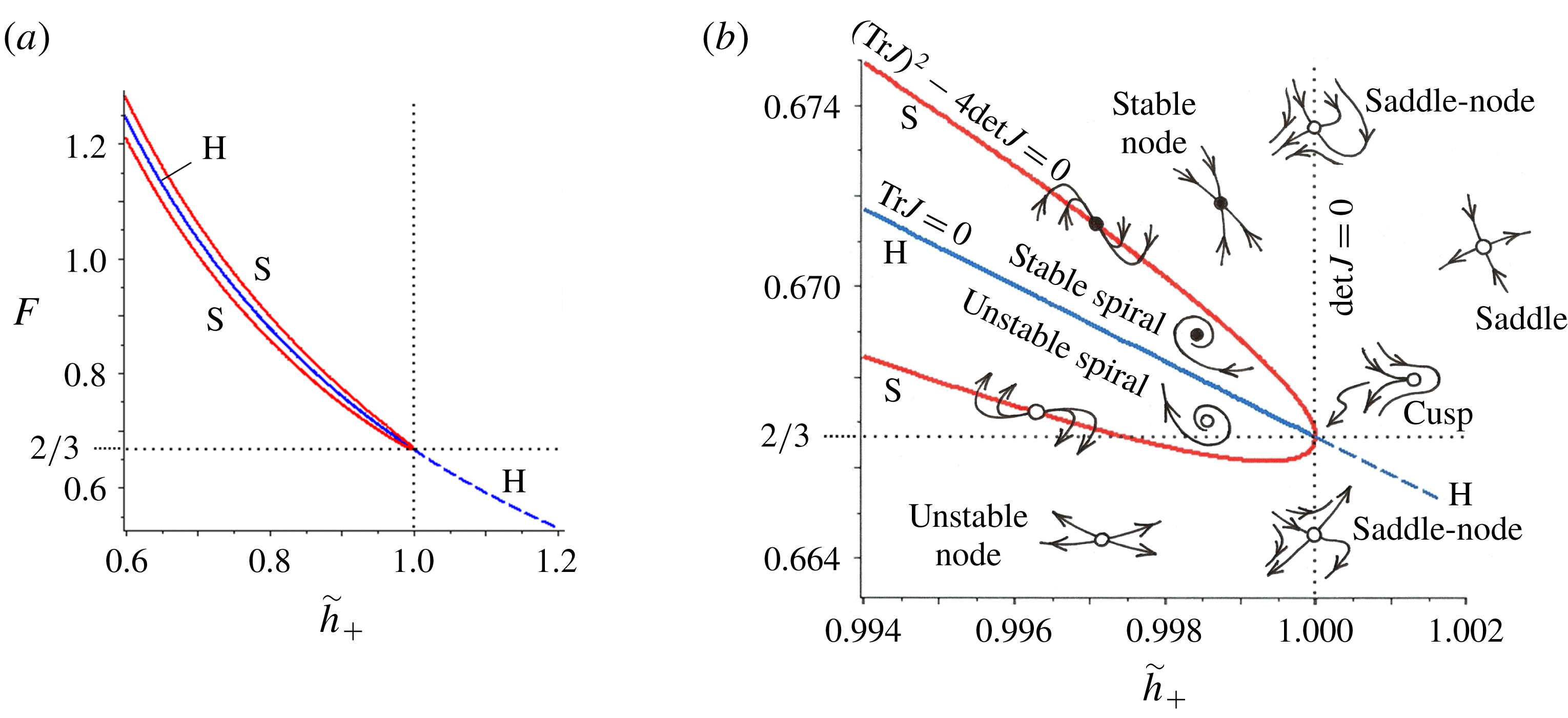
exhibit a particularly interesting behaviour. This is illustrated in figure 3, where we have plotted the
 $(\tilde{h}_{+},F)$
parameter space in the vicinity of the critical point
 $(\tilde{h}_{+},F)=(1,2/3)$
; first on a relatively large scale and also a detailed view of the immediate neighbourhood of
 $(\tilde{h}_{+},F)=(1,2/3)$
. We see several curves, which all intersect at the critical point, each of them playing an important role in the classification of the fixed point
 $(1,0)$
. Indeed, this parameter diagram shows how the nature of this fixed point changes with varying control parameters
 $\tilde{h}_{+}$
and
 $F$
, and is to be compared with the standard classification scheme – obtained from linear stability analysis – for the fixed points of two-dimensional dynamical systems (Strogatz Reference Strogatz1994, see § 8.4 in particular).
Apart from the division line
 $F=2/3$
(being the threshold of instability for the uniform flow and the monoclinal wave), the two central lines of this diagram are the curves along which the determinant and trace of the Jacobian matrix
 $\unicode[STIX]{x1D645}_{(1,0)}$
are zero. The first of these is the vertical line
 $\tilde{h}_{+}=1$
(where
 $\text{det}\,J_{(1,0)}=0$
) and the second one is the curve denoted by ‘H’ (where
 $TrJ_{(1,0)}=0$
).
Two views of the
 $(\tilde{h}_{+},F)$
parameter space, for
 $\unicode[STIX]{x1D701}=33.3^{\circ }$
, showing the linear stability properties of the fixed point
 $(1,0)$
, as dictated by the eigenvalues (3.21): (a) the extended vicinity of the critical point
 $(\tilde{h}_{+},F)=(1,2/3)$
, and (b) the immediate neighbourhood of the same critical point. Several zones can be distinguished, and in each of these the local dynamics of the fixed point
 $(1,0)$
is sketched. In the region enclosed by the curve ‘S’, given by (3.26), the fixed point is a spiral, whereas below/above this region it is an unstable/stable node. The extended view of the
 $(\tilde{h}_{+},F)$
space shows that
 $(1,0)$
assumes the form of a spiral only in a narrow strip around the Hopf bifurcation line ‘H’. The latter line, given by (3.24), divides the enclosed region in a zone where
 $(1,0)$
is an unstable spiral (below ‘H’) and one where it is a stable spiral (above ‘H’). Along the vertical line
 $\tilde{h}_{+}=1$
the fixed point
 $(1,0)$
is of hybrid type (a saddle–node for all
 $F\neq 2/3$
and a cusp for
 $F=2/3$
) and for
 $\tilde{h}_{+}>1$
it takes the form of a saddle.

For the first line,
 $\tilde{h}_{+}=1$
, one may easily verify that
 $\text{det}\,J_{(1,0)}=0$
. Indeed, the value
 $\tilde{h}_{+}=1$
corresponds to
 $\tilde{c}=5/2$
, cf. (3.11), and for this value the determinant given by (3.17a
) vanishes.
The line ‘H’ in figure 3 is found by requiring that the trace
 $TrJ_{(1,0)}$
must be zero. From (3.17b
) we can see that this implies
 $1-F^{2}[\tilde{c}(\tilde{h}_{+})-1]^{2}=0$
, which gives
 $\tilde{c}(\tilde{h}_{+})=1\pm 1/F$
. Since
 $\tilde{c}$
is always larger than
 $1$
, we thus arrive at the elegant expression
 $$\begin{eqnarray}\tilde{c}(\tilde{h}_{+})=1+\frac{1}{F},\quad \text{along `H'}.\end{eqnarray}$$
This same relation was also found by Gray & Edwards (Reference Gray and Edwards2014) in their analysis of the birth of roll waves from the destabilized uniform flow. With the aid of (3.11) we substitute the wave speed
 $\tilde{c}$
by the expression
 $(1-\tilde{h}_{+}^{5/2})/(1-\tilde{h}_{+})$
and find
 $$\begin{eqnarray}F=\frac{1-\tilde{h}_{+}}{\tilde{h}_{+}(1-\tilde{h}_{+}^{3/2})},\quad \text{along `H'},\end{eqnarray}$$
which defines the line ‘H’ in the
 $(\tilde{h}_{+},F)$
plane of figure 3.
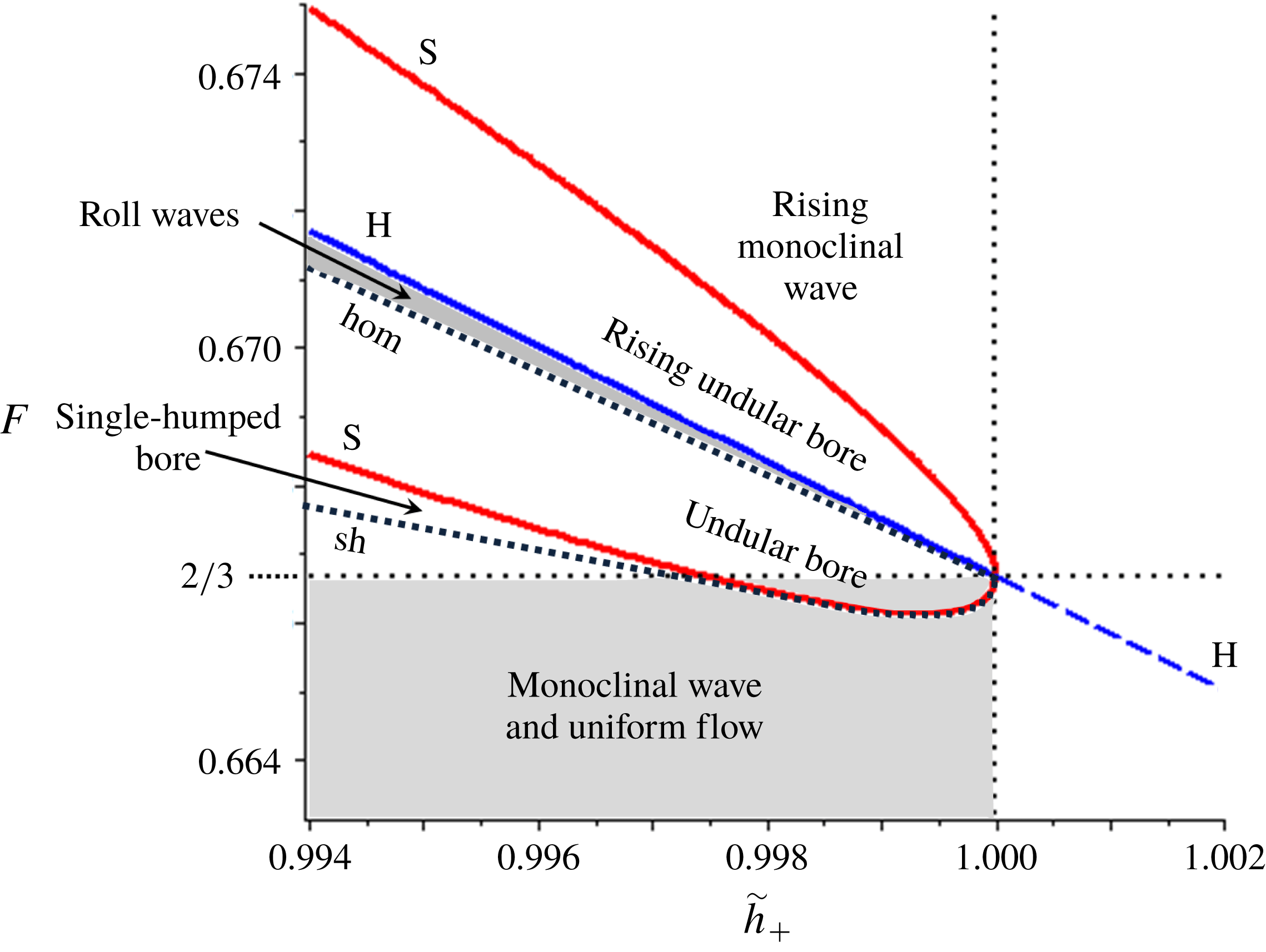
Another significant line in the parameter space is the rounded curve ‘S’, which defines the boundary of the region where the fixed point
 $(1,0)$
is a spiral point. It is determined by setting the expression under the square root of the eigenvalues
 $\unicode[STIX]{x1D706}_{a,b}^{(1,0)}(\tilde{h}_{+},F,\unicode[STIX]{x1D701})$
in (3.21) equal to zero. At this instant the two eigenvalues coincide on the real axis and they are on the edge between a node (with two real eigenvalues of the same sign) and a spiral (for which the two eigenvalues form a complex conjugate pair). This condition can be written as
 $$\begin{eqnarray}9(1-F^{2}(\tilde{c}-1)^{2})^{2}+4\unicode[STIX]{x1D6E4}(\unicode[STIX]{x1D701})\tan \unicode[STIX]{x1D701}(\tilde{c}-1)(2\tilde{c}-5)=0,\quad \text{along `S'},\end{eqnarray}$$
or (keeping only positive values of
 $F$
)
 $$\begin{eqnarray}F=\frac{1}{(\tilde{c}-1)}\sqrt{1\pm \frac{2}{3}\sqrt{\unicode[STIX]{x1D6E4}(\unicode[STIX]{x1D701})\tan \unicode[STIX]{x1D701}(\tilde{c}-1)(5-2\tilde{c})}},\quad \text{along `S'}.\end{eqnarray}$$
This is the analytical relation between
 $F$
and
 $\tilde{c}$
(or equivalently, between
 $F$
and
 $\tilde{h}_{+}$
, employing again (3.11) for
 $\tilde{c}(\tilde{h}_{+})$
) yielding the curve ‘S’ in the
 $(\tilde{h}_{+},F)$
parameter space.
In the region enclosed by the curve ‘S’, the fixed point
 $(1,0)$
is a spiral point, i.e. its eigenvalues form a complex conjugate pair. Below the region in question, both eigenvalues lie on the positive real axis, meaning that
 $(1,0)$
is an unstable node. Above the enclosed region (i.e. in the narrow space between ‘S’ and the vertical line
 $\tilde{h}_{+}=1$
for
 $F>2/3$
) the eigenvalues lie on the negative real axis, hence
 $(1,0)$
is a stable node there. On the curve ‘S’ itself, the fixed point is a degenerate node on the threshold of becoming a spiral.
For future reference we note that, for the system parameters chosen in this paper, the lowest point of the curve ‘S’ lies at
 $F=F_{und}=0.66614265$
and
 $\tilde{h}_{+}=0.999371$
. So this is the lowest Froude number for which the fixed point
 $(1,0)$
can become a spiral. In the next sections we will see that this – when the fixed point turns into a spiral – heralds the appearance of undulations on the surface of the granular sheet, which introduces a novel type of wave, the granular undular bore, and constitutes a necessary first step towards the development of roll waves. This also explains the subscript in the parameter
 $F_{und}$
, which stands for ‘undular’.
The curve ‘H’ is seen to divide the region bounded by the curve ‘S’ into two subregions: (i) the area below ‘H’, where the spiral point
 $(1,0)$
is unstable, and (ii) the area above ‘H’, where
 $(1,0)$
is a stable spiral point. Along ‘H’ itself, the two eigenvalues are purely imaginary and the local stability properties of
 $(1,0)$
are those of a centre point. At this instant the point
 $(1,0)$
undergoes a reverse Hopf bifurcation, as we will see in § 4.4, and this event turns out to be directly related to the appearance of roll waves in the system. Indeed, it is because of this Hopf bifurcation that we have assigned the letter ‘H’ to the curve in question.
With regards to the part of ‘H’ lying outside the region enclosed by ‘S’ (the part in figure 3 which is dashed), the two eigenvalues are real and of opposite sign, having the same magnitude. So here the fixed point
 $(1,0)$
is a saddle. In fact, it is a saddle in the entire region
 $\tilde{h}_{+}>1$
, because everywhere in this area the two eigenvalues
 $\unicode[STIX]{x1D706}_{a}^{(1,0)}(\tilde{h}_{+},F,\unicode[STIX]{x1D701})$
are real and of opposite sign (although not of equal magnitude except on ‘H’). The fact that
 $(1,0)$
is a saddle for
 $\tilde{h}_{+}>1$
is immediately related to the exchange of roles between the two fixed points
 $(1,0)$
and
 $(\tilde{h}_{+},0)$
, which was discussed in the context of (3.15). As explained there, no new physics is found in the region
 $\tilde{h}_{+}>1$
, so we restrict ourselves to the left part of the diagram (
 $\tilde{h}_{+}\leqslant 1$
).
Based on figure 3, we will scan the parameter space following paths of two different types, in the horizontal and vertical directions respectively: (i) in § 4 we vary
 $\tilde{h}_{+}$
while keeping
 $F$
fixed (at some value close to the critical Froude number
 $2/3$
) and (ii) in § 5 we vary
 $F$
while keeping
 $\tilde{h}_{+}$
fixed (at some value close to
 $1$
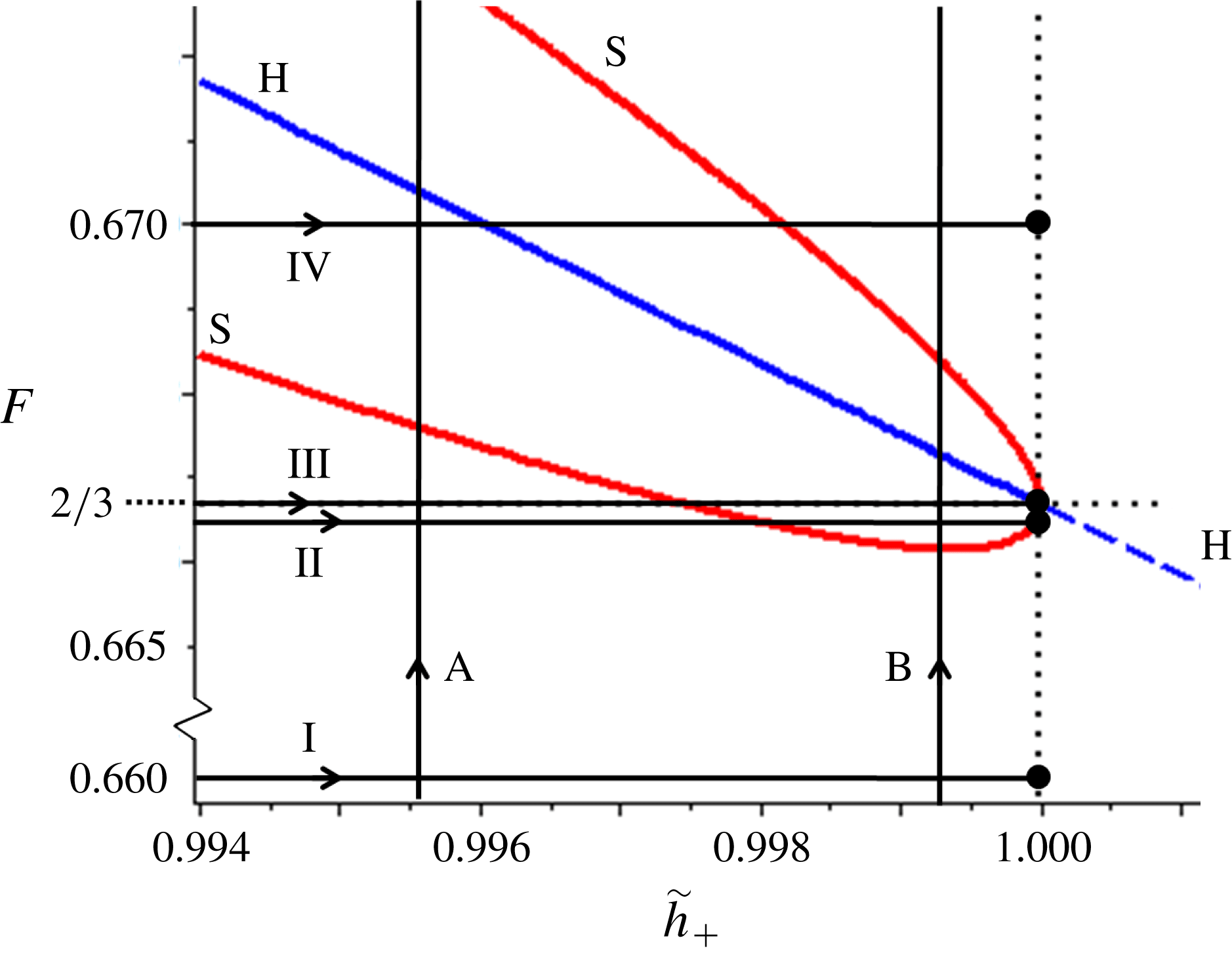
). These paths are depicted in figure 4, which will serve as a roadmap for the next two sections.
The paths through the
 $(\tilde{h}_{+},F)$
parameter space that are followed in §§ 4 and 5. The horizontal paths denoted by roman numerals are chosen such that each of them makes a qualitatively different cut through the regions defined by the curves ‘H’ and ‘S’. These paths end at the value
 $\tilde{h}_{+}=1$
, corresponding to uniform flow conditions that are either stable (for
 $F<2/3$
), critical (
 $F=2/3$
) or unstable (
 $F>2/3$
). The vertical paths denoted by the letters A and B follow the sequence of events when, for a fixed
 $\tilde{h}_{+}$
(constant ratio between the thicknesses of outflow and inflow), we raise the Froude number of the incoming flow.

4 A phase-plane view of the various waveforms
In this section we vary the thickness
 $\tilde{h}_{+}$
while keeping the Froude number of the incoming flow
 $F$
fixed. We will do this for four representative values of
 $F$
close to
 $2/3$
, along the horizontal lines I–IV of figure 4. The range through which
 $\tilde{h}_{+}$
is varied runs from the threshold value
 $\tilde{h}_{+,min}=\unicode[STIX]{x1D6FD}/F$
(corresponding to the thickness below which the sheet develops stopping regions) up to
 $1$
. For each path, we follow the trajectories of the eigenvalues
 $\unicode[STIX]{x1D706}_{a,b}^{(1,0)}(\tilde{h}_{+},F,\unicode[STIX]{x1D701})$
in the complex plane and, at several characteristic stages (indicated by a, b, etc. in the topmost plots of figures 5, 6, 7 and 8), we plot the phase portraits and the associated waveforms on the granular sheet. The eigenvalue pairs (3.20) and (3.21) determine the linear stability properties of the fixed points
 $(\tilde{h}_{+},0)$
and
 $(1,0)$
, respectively, and thereby govern the local behaviour around them. We now supplement this local view by drawing the full phase-plane portraits, which reveal also the global behaviour of our dynamical system (3.12).
The light grey arrows in the background of the phase portraits correspond to the direction field
 $d\tilde{s}/d\tilde{h}$
of the dynamical system. And the trajectories in this same
 $(\tilde{h},\tilde{s})$
-plane show how the height and slope evolve as a function of
 $\tilde{\unicode[STIX]{x1D709}}$
. Many trajectories are seen to wander off (either to large
 $\tilde{h}$
-values with an increasingly positive slope, or in the opposite direction with a negative slope), corresponding to diverging solutions that are of little relevance for experiments. Yet close to the two fixed points
 $(\tilde{h}_{+},0)$
and
 $(1,0)$
we also find trajectories that do not escape to infinity, and these correspond to the waveforms for which we are looking.
For a proper interpretation of the phase portraits, one should keep in mind that the arrows point in the positive
 $\tilde{\unicode[STIX]{x1D709}}$
direction, i.e. in the downstream direction in the co-moving frame. So the phase space trajectories trace out the profile of
 $\tilde{h}(\tilde{\unicode[STIX]{x1D709}})$
and
 $\tilde{s}(\tilde{\unicode[STIX]{x1D709}})$
in the downstream direction. The same trajectories can also be used to infer how the sheet rises or falls at any given position
 $\tilde{x}=\tilde{x}_{0}$
as a function of time, but in this case one has to follow the arrows backwards. This is because of the minus sign in
 $\tilde{\unicode[STIX]{x1D709}}=\tilde{x}-\tilde{c}\tilde{t}$
, which means that the time variable runs in the opposite direction of
 $\tilde{\unicode[STIX]{x1D709}}$
. Specifically, at point
 $\tilde{x}=\tilde{x}_{0}$
we have
 $\tilde{t}=(\tilde{x}_{0}-\tilde{\unicode[STIX]{x1D709}})/\tilde{c}$
. Both views, forward in
 $\tilde{\unicode[STIX]{x1D709}}$
(following the arrows) and forward in
 $\tilde{t}$
(against the arrows), will be used in our analysis.
At each of the four
 $F$
-values considered, for
 $\tilde{h}_{+,min}=\unicode[STIX]{x1D6FD}/F$
the eigenvalues
 $\unicode[STIX]{x1D706}_{a,b}^{(1,0)}(\tilde{h}_{+},F,\unicode[STIX]{x1D701})$
start out from two points on the positive real axis, and for
 $\tilde{h}_{+}=1$
they end at the same values as those given by (3.22a–c
) of the other fixed point
 $(\tilde{h}_{+},0)$
; this stands to reason, since for
 $\tilde{h}_{+}=1$
the two fixed points coincide. In between, their behaviour depends in an interesting way on
 $F$
, as we will now show.
4.1 Path I. The domain of monoclinal waves
For
 $F$
sufficiently smaller than the critical value
 $2/3$
(in particular, smaller than the value
 $F_{und}=0.66614265$
at the lower tip of the region enclosed by the curve ‘S’ in figures 3 and 4) the eigenvalues
 $\unicode[STIX]{x1D706}_{a,b}^{(1,0)}(\tilde{h}_{+},F,\unicode[STIX]{x1D701})$
never meet each other and simply move along the positive real axis. This is illustrated in figure 5 for
 $F=0.6600$
, which despite its closeness to
 $2/3$
is already sufficiently small.
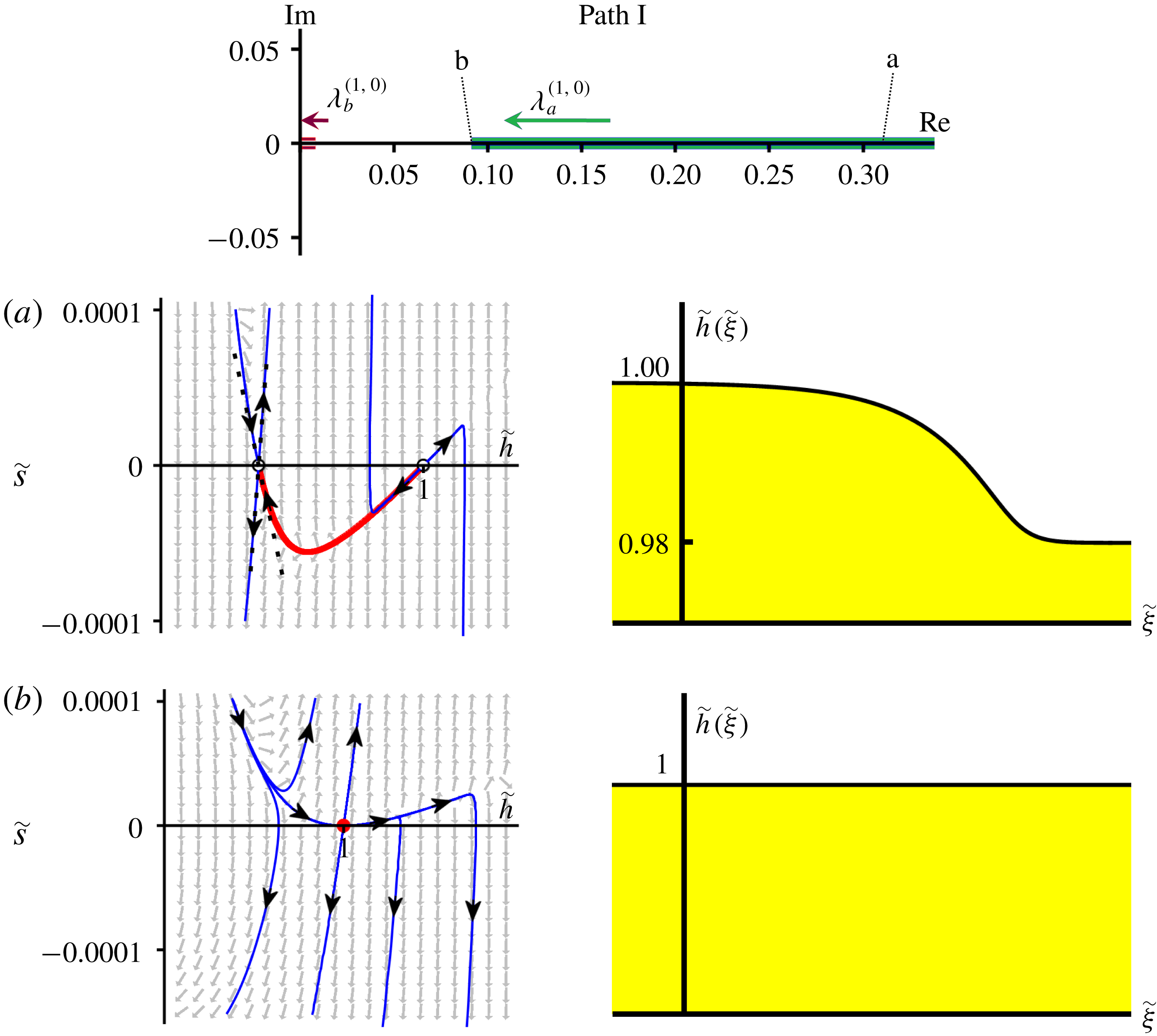
Path I. Trajectories in the complex plane of the two eigenvalues
 $\unicode[STIX]{x1D706}_{a,b}^{(1,0)}(\tilde{h}_{+},F,\unicode[STIX]{x1D701})$
, see (3.21), as
 $\tilde{h}_{+}$
is varied from
 $\unicode[STIX]{x1D6FD}/F$
to
 $1$
, at fixed
 $F=0.6600<F_{und}$
. At this value of
 $F$
, the eigenvalues never leave the positive real axis, so the fixed point
 $(1,0)$
remains an unstable node; it only turns into a hybrid saddle–node point when
 $\tilde{h}_{+}$
reaches
 $1$
. The phase portraits clarify the granular waveforms encountered on the chute. (a) For
 $\tilde{h}_{+}=0.98$
the fixed points
 $(\tilde{h}_{+},0)$
and
 $(1,0)$
, a saddle and an unstable node respectively, are seen to be connected by a heteroclinic orbit (thick red curve) representing a monoclinal wave, as shown by the accompanying profile
 $\tilde{h}(\tilde{\unicode[STIX]{x1D709}})$
. (b) When
 $\tilde{h}_{+}$
reaches
 $1$
the saddle and the unstable node merge, creating a single fixed point of hybrid nature, combining the characteristics of a saddle with those of an unstable node (cf. figure 3
b along the vertical axis
 $\tilde{h}_{+}=1$
for
 $F<2/3$
). The levels of inflow (
 $\tilde{h}_{-}=1$
) and outflow
 $\tilde{h}_{+}$
are now equally high and the monoclinal wave reduces to a uniform flow, represented by the horizontal profile
 $\tilde{h}(\tilde{\unicode[STIX]{x1D709}})$
of height
 $1$
.

The fact that the eigenvalues stay on the positive real axis implies that the fixed point
 $(1,0)$
remains an unstable node for all
 $\unicode[STIX]{x1D6FD}/F<\tilde{h}_{+}<1$
. In figure 5(a) we give the corresponding phase portrait at the characteristic value of
 $\tilde{h}_{+}=0.98$
. The two fixed points
 $(\tilde{h}_{+},0)$
and
 $(1,0)$
, being a saddle and an unstable node respectively, are clearly visible. The heteroclinic connection between them (highlighted as a thick red curve) corresponds to the stable monoclinal waveform that links the two regions of uniform flow with heights
 $\tilde{h}_{-}=1$
and
 $\tilde{h}_{+}=0.98$
, given by the accompanying profile
 $\tilde{h}(\tilde{\unicode[STIX]{x1D709}})$
.
In order to understand how an unstable node (and a saddle) can be related to a stable monoclinal wave, we recall that the arrows in the phase plane (which point in the direction of growing
 $\tilde{\unicode[STIX]{x1D709}}$
) should be followed in the opposite direction if one wishes to examine the temporal evolution (i.e. for growing
 $\tilde{t}$
) at a given position along the chute. Therefore, the unstable node
 $(1,0)$
represents an attracting point when viewed as a function of
 $\tilde{t}$
at the position
 $\tilde{x}=\tilde{x}_{0}$
: starting from initial conditions
 $\tilde{h}(\tilde{x}_{0},0)$
and
 $\tilde{s}(\tilde{x}_{0},0)$
sufficiently close to
 $(\tilde{h},\tilde{s})=(1,0)$
, the granular sheet will eventually acquire uniform flow conditions with
 $\tilde{h}(\tilde{x}_{0},\tilde{t})\rightarrow \tilde{h}_{-}=1$
and
 $\tilde{s}(\tilde{x}_{0},\tilde{t})\rightarrow 0$
.
In the limiting case
 $\tilde{h}_{+}=1$
, the eigenvalue
 $\unicode[STIX]{x1D706}_{b}^{(1,0)}(\tilde{h}_{+},F,\unicode[STIX]{x1D701})$
becomes zero, rendering the node degenerate. At the same time, the second fixed point
 $(\tilde{h}_{+},0)$
merges with
 $(1,0)$
and turns into a degenerate saddle, because its eigenvalue
 $\unicode[STIX]{x1D706}_{b}^{(\tilde{h}_{+},0)}(\tilde{h}_{+},F,\unicode[STIX]{x1D701})$
(which up to then had been negative) becomes zero (cf. (3.22a
)). The result is that the fixed point
 $(1,0)$
is now of a hybrid saddle–node type, with one eigenvalue being zero and the other one real and positive, bearing the characteristics of both an unstable node and a saddle. This is illustrated in figure 5(b) for
 $\tilde{h}_{+}=1$
, where we show the phase portrait featuring the hybrid fixed point, as well as the corresponding profile
 $\tilde{h}(\tilde{\unicode[STIX]{x1D709}})$
with the levels of inflow and outflow being equally high. This means that the amplitude of the monoclinal wave vanishes and the flow reduces to a uniformly flat one.
The physical interpretation of the zero eigenvalue that the node acquires when
 $\tilde{h}_{+}$
becomes equal to
 $\tilde{h}_{-}=1$
is that the uniformly flowing sheet (with
 $\tilde{h}_{+}=\tilde{h}_{-}$
) is invariant for any small uniform increase or decrease of its thickness. The other eigenvalue acquires the value
 $\unicode[STIX]{x1D706}_{a}^{(1,0)}(1,F,\unicode[STIX]{x1D701})=(3/\tan \unicode[STIX]{x1D701})[1-(9/4)F^{2}]$
, which is positive since
 $F<2/3$
. This corresponds to a stable temporal behaviour, meaning that at these values of
 $F$
small perturbations to the uniform flow will be smoothed out with time.
4.2 Path II. Appearance of a novel stable waveform: the granular undular bore
For
 $F$
closer to
 $2/3$
, but still slightly below this value, the eigenvalues meet each other and leave the real axis. This happens when the expression under the square root in (3.21) vanishes at this point, which defines the curve ‘S’ in the
 $(\tilde{h}_{+},F)$
parameter space. For the parameter values used in this paper, the smallest value of
 $F$
for which this is possible is
 $F=F_{und}=0.66614265$
, and the corresponding height of the outgoing flow is
 $\tilde{h}_{+}=0.999371$
, i.e. only slightly smaller than the unit height of the incoming flow. These values correspond to the coordinates of the lowest point of curve ‘S’ in figures 3 and 4.
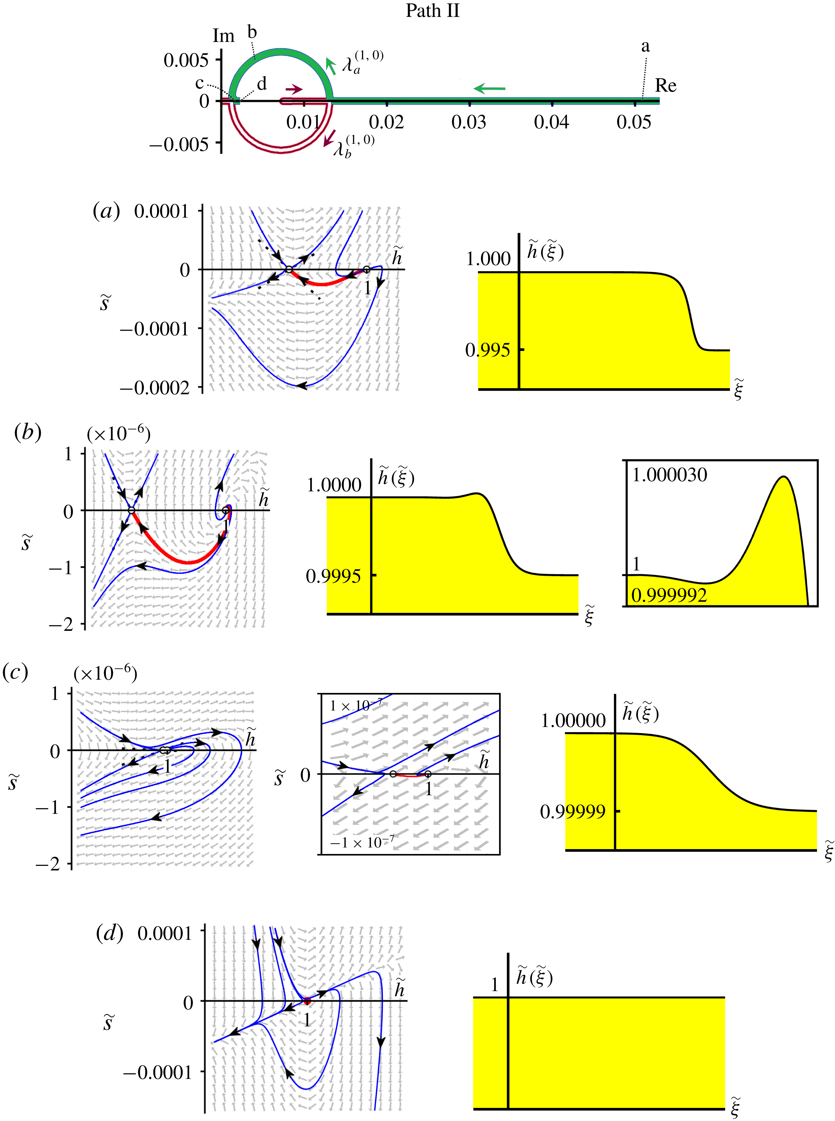
In figure 6 we draw the phase plane for the typical value
 $F=0.6665$
. We see that the eigenvalues indeed leave the real axis and temporarily form a complex conjugate pair, which means that
 $(1,0)$
becomes an (unstable) spiral point. This is in full agreement with figure 3. The eigenvalues follow semicircular trajectories before rejoining each other on the real axis, and then move in opposite directions along the positive real axis until
 $\tilde{h}_{+}$
reaches
 $1$
.
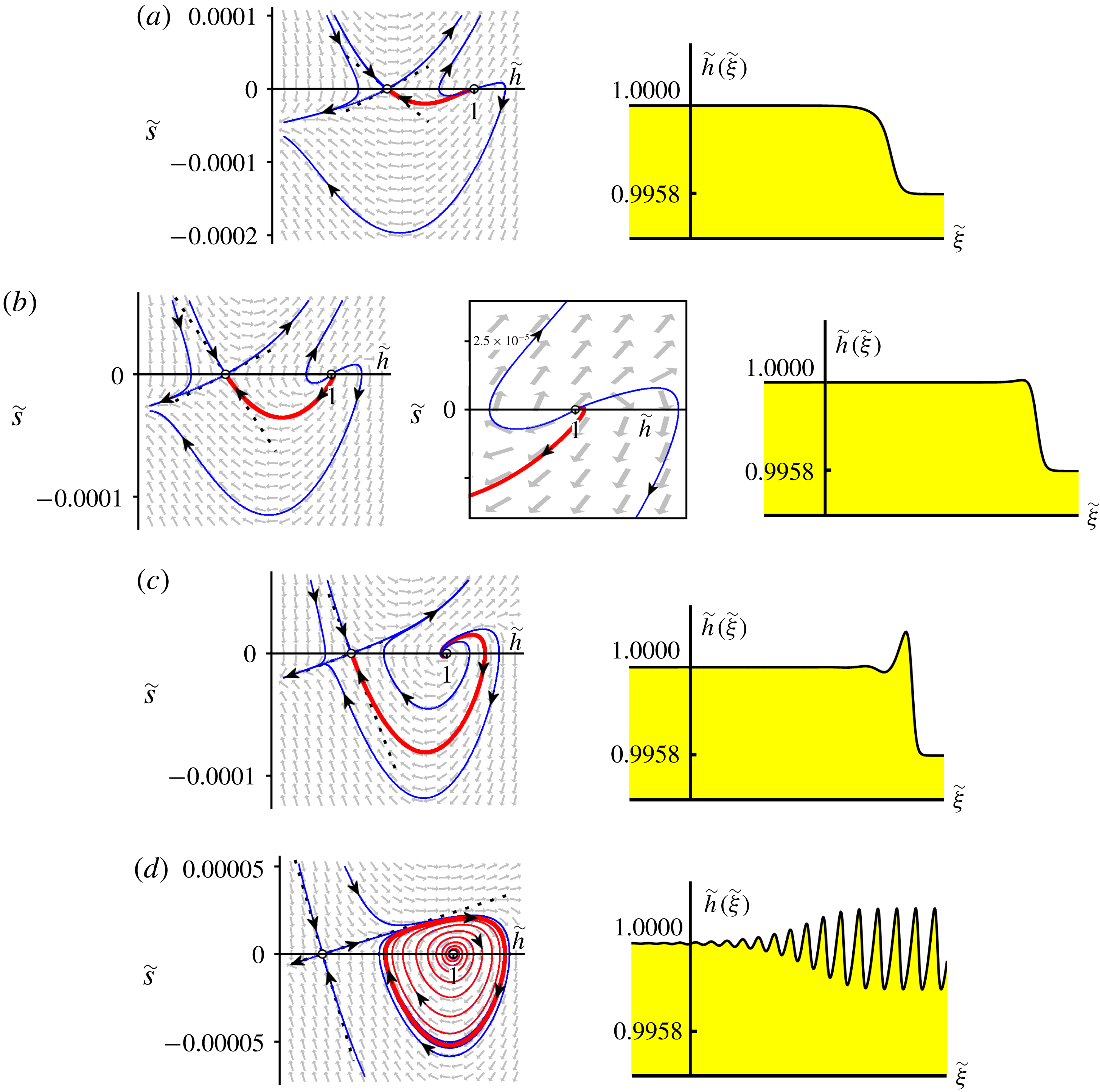
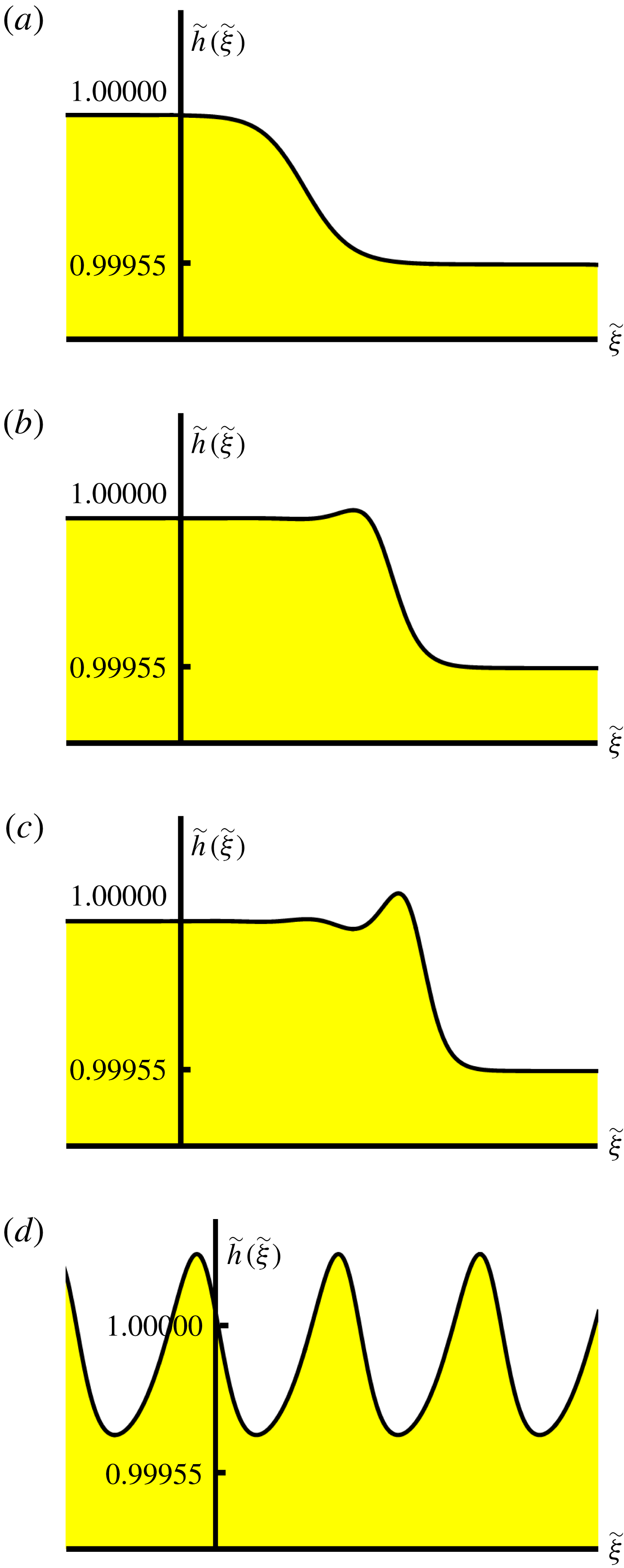
The plots in figure 6 illustrate four successive stages of this sequence of events. For
 $\tilde{h}_{+}=0.995$
(stage a), the fixed point at
 $(1,0)$
is still an unstable node, and the heteroclinic connection with the saddle point
 $(\tilde{h}_{+},0)$
constitutes a monoclinal shock structure as before.
In the very last stages before reaching line ‘S’, the monoclinal nature will be violated – very slightly – by the appearance of a subtle hump (too small to be visible) at the top of the wave. This means that the slope
 $d\tilde{h}/d\tilde{\unicode[STIX]{x1D709}}$
is no longer strictly negative along the entire wave profile. In the phase portrait, the connection between
 $(1,0)$
and the saddle point is then established via the unstable manifold emanating from
 $(1,0)$
towards the northeast (instead of via the twin manifold in the southwest). The corresponding waveform is a single-humped (non-monoclinal) bore.
In the next plot, for
 $\tilde{h}_{+}=0.9995$
(figure 6
b), we have crossed the curve ‘S’ of figures 3 and 4 and the fixed point
 $(1,0)$
has become an unstable spiral. The heteroclinic orbit now winds around
 $(1,0)$
and this spiralling motion in the phase plane corresponds to a series of undulations in the height profile
 $\tilde{h}(\tilde{\unicode[STIX]{x1D709}})$
; the undulations are highlighted by means of a close-up. (Throughout this paper we will often adjust the scales of the phase portraits and profiles so as to focus upon the region of interest.) Clearly, the slope
 $d\tilde{h}/d\tilde{\unicode[STIX]{x1D709}}$
is no longer monotonically negative along the entire chute, so this waveform is not a monoclinal wave. In fact, it is an undular bore, which – as mentioned before – is a new waveform as far as granular flows are concerned.
In water, by contrast, the undular bore is a familiar phenomenon (Peregrine Reference Peregrine1966; Benjamin, Bona & Mahony Reference Benjamin, Bona and Mahony1972; Whitham Reference Whitham1974; Chanson Reference Chanson2011; Fowler Reference Fowler2011; Bonneton et al.
Reference Bonneton, Filippini, Arpaia, Bonneton and Ricchiuto2016; Rousseaux et al.
Reference Rousseaux, Mougenot, Chatellier, David and Calluaud2016). Chanson (Reference Chanson2011) reports that more than
 $400$
estuaries around the globe are affected by tidal bores. Spectacular examples include the famous Severn bore in the United Kingdom, the ‘mascaret’ on the rivers Dordogne and Sélune in France and the Pororoca on the Amazon.
The fact that in granular flows they have remained undetected so far may be attributed to their small amplitude. In the numerical experiment we are performing here, the difference between
 $\tilde{h}_{-}=1$
and
 $\tilde{h}_{+}$
is only
 $0.0005$
, and the amplitude of the undulation itself is of the order of
 $4\,\%$
of this, corresponding to only a fraction of the diameter of a granular particle. Given the smallness of these numbers, it is not surprising that the granular undular bore has escaped detection up to now. Mathematically, however, it is an indispensable intermediate stage between the demise of the monoclinal wave and the rise of roll waves; we will come back to this point later.
Path II. Trajectories of the eigenvalues
 $\unicode[STIX]{x1D706}_{a,b}^{(1,0)}$
, with phase portraits and wave profiles, for
 $F=0.6665$
(between
 $F_{und}=0.66614265$
and
 $2/3$
). (a) For
 $\tilde{h}_{+}=0.995$
,
 $(1,0)$
is an unstable node. Its connection with the saddle
 $(\tilde{h}_{+},0)$
constitutes a monoclinal wave. (b) At
 $\tilde{h}_{+}=0.9995$
the eigenvalues have left the real axis and form a complex conjugate pair, turning
 $(1,0)$
into an unstable spiral. The heteroclinic orbit spirals around
 $(1,0)$
, causing
 $\tilde{h}(\tilde{\unicode[STIX]{x1D709}})$
to take the form of an undular bore (cf. close-up). (c) At
 $\tilde{h}_{+}=0.99999$
,
 $\unicode[STIX]{x1D706}_{a,b}^{(1,0)}$
have returned to the positive real axis so
 $(1,0)$
is an unstable node again. The heteroclinic orbit (cf. blow-up of the phase portrait) corresponds to a monoclinal wave of minute amplitude. (d) Finally, at
 $\tilde{h}_{+}=1$
the saddle and node merge, creating a hybrid saddle–node just as in figure 5(b); the associated profile is a – still stable – uniform flow.

Before leaving the topic, let us mention an intriguing similarity between the undular bore described here and the ripples on the granular jump studied by Boudet et al. (Reference Boudet, Amarouchene, Bonnier and Kellay2007). Those authors analyse the granular analogue of a hydraulic jump, which is formed when a jet of fine sand impinges on a solid horizontal surface. The sand flows radially outwards in the form of a thin rapid sheet, until it comes to rest at a certain distance from the point of impact, where it creates a thicker deposition annulus. The inner rim of this annulus closes in upon the jet, in a shock-like fashion resembling the granular bore of the present paper. That is, the widening deposition annulus exhibits undulations; see figures 1(c) and 10 in Boudet et al. (Reference Boudet, Amarouchene, Bonnier and Kellay2007). These undulations, however, are stationary in contrast to the travelling undulations of the bore analysed here.
In the next stage, at
 $\tilde{h}_{+}=0.99999$
(figure 6
c), the eigenvalues have come back to the positive real axis and
 $(1,0)$
is an unstable node once more. The heteroclinic connection no longer spirals out from
 $(1,0)$
, and the waveform is monoclinal again. In figure 3 we now find ourselves between the curve ‘S’ and the vertical axis
 $\tilde{h}_{+}=1$
.
Finally, when
 $\tilde{h}_{+}$
reaches
 $1$
(figure 6
d), the saddle and unstable node merge to produce a single fixed point of hybrid saddle–node type. The corresponding profile
 $\tilde{h}(\tilde{\unicode[STIX]{x1D709}})$
is a sheet of uniform height
 $1$
. Moreover, it is still stable to small perturbations of its thickness, though only just, because we are very close to the critical Froude number
 $2/3$
.
Path III. For the critical value
 $F=2/3$
, the semicircular trajectories of the eigenvalues
 $\unicode[STIX]{x1D706}_{a,b}^{(1,0)}$
meet at the origin of the complex plane precisely when
 $\tilde{h}_{+}=1$
. The initial stages, illustrated here for (a)
 $\tilde{h}_{+}=0.995$
and (b)
 $0.9995$
, resemble those of figure 6. The difference lies in the final stage for (c)
 $\tilde{h}_{+}=1$
, when the spiral
 $(1,0)$
and the saddle
 $(\tilde{h}_{+},0)$
merge to produce a cusp, highlighted also in close-up. This cusp, corresponding to the multicritical point
 $(\tilde{h}_{+},F)=(1,2/3)$
of figure 3, represents the pivotal point around which the transition from monoclinal waves to roll waves is organized. The associated profile
 $\tilde{h}(\tilde{\unicode[STIX]{x1D709}})$
is a marginally stable uniform flow.

4.3 Path III. The critical case
 $F=2/3$

If the Froude number of the incoming flow equals
 $2/3$
, a granular sheet of uniform thickness becomes prone to the so-called Kapitza instability, also called the long-surface-wave instability or roll wave instability (Kapitza & Kapitza Reference Kapitza and Kapitza1949; Forterre & Pouliquen Reference Forterre and Pouliquen2003; Forterre Reference Forterre2006; Aranson & Tsimring Reference Aranson and Tsimring2009, see § 6.4 in particular; Andreotti et al.
Reference Andreotti, Forterre and Pouliquen2013, see chap. 6 in particular; Gray & Edwards Reference Gray and Edwards2014). In our description, this instability enters the scene in the special way in which critical phenomena manifest themselves in dynamical systems, namely via the appearance of a degenerate fixed point. At
 $F=2/3$
, the semicircular trajectories of the eigenvalues
 $\unicode[STIX]{x1D706}_{a,b}^{(1,0)}(\tilde{h}_{+},F,\unicode[STIX]{x1D701})$
meet each other exactly at the origin of the complex plane when
 $\tilde{h}_{+}=1$
. At this instant, the unstable spiral
 $(1,0)$
and the saddle
 $(\tilde{h}_{+},0)$
merge to create a single fixed point – at
 $(1,0)$
– with a double zero eigenvalue. This means that the linear stability analysis no longer provides a picture of the dynamics around the fixed point. It only says that it is marginally stable as far as the linear stability goes, and that the tiniest perturbation is sufficient to tip the balance. The numerically generated phase portrait in figure 7(c) shows that the fixed point is now a cusp.
The full sequence of events is illustrated in figure 7. The first stages are similar to those of figure 6(a,b). However, the final plot for
 $\tilde{h}_{+}=1$
is different. Here the saddle
 $(\tilde{h}_{+},0)$
and the spiral point
 $(1,0)$
merge, with all eigenvalues becoming simultaneously zero, as can be checked from (3.20) and (3.21) (cf. (3.22b
)). The point created by the merger is a cusp, as mentioned above, and the corresponding profile
 $\tilde{h}(\tilde{\unicode[STIX]{x1D709}})$
is a marginally stable uniform flow. Any small addition of material will cause a breakdown of the flat profile and trigger the eventual emergence of a train of roll waves.
4.4 Path IV. The emergence of roll waves for
$F>2/3$

We now come to the case when the Froude number
 $F$
of the incoming flow exceeds the critical value
 $2/3$
. Here we find the richest sequence of events, and it is here that we will encounter roll waves.
Taking
 $F=0.67$
as a representative value, the trajectories of the eigenvalues
 $\unicode[STIX]{x1D706}_{a,b}^{(1,0)}$
and the corresponding phase-plane portraits and wave profiles are presented in figure 8. We observe that the semicircular paths of
 $\unicode[STIX]{x1D706}_{a,b}^{(1,0)}$
are larger than previously and now intersect the imaginary axis before
 $\tilde{h}_{+}$
has reached
 $1$
. The eigenvalues are then purely imaginary, corresponding to a reverse Hopf bifurcation in which the spiral point
 $(1,0)$
is stabilized and the limit cycle (associated with a roll wave) is annihilated.
Path IV. Trajectories of the eigenvalues
 $\unicode[STIX]{x1D706}_{a,b}^{(1,0)}$
for
 $F=0.67>2/3$
, at successive values of
 $\tilde{h}_{+}$
indicated in the profile plots. The semicircular paths have expanded further and now intersect the imaginary axis before
 $\tilde{h}_{+}$
has reached
 $1$
. This intersection is associated with a reverse Hopf bifurcation in which the spiral point
 $(1,0)$
turns stable. Subsequently, the eigenvalues proceed along their paths, meeting each other on the negative real axis (transforming
 $(1,0)$
into a stable node) and then move along this axis in opposite directions. The first two stages depicted here, (a) when the eigenvalues are still on the positive real axis and (b) after they have left it, show a single-humped bore and its undular variety, respectively. The former will be analysed in detail in § 5. Preceding the reverse Hopf bifurcation (while
 $\unicode[STIX]{x1D706}_{a,b}^{(1,0)}$
are still complex conjugate with a positive real part) a new phenomenon occurs: (c) for
 $\tilde{h}_{+}=0.995592$
the stable and unstable manifolds of the saddle
 $(\tilde{h}_{+},0)$
smoothly join onto each other, forming a closed homoclinic orbit; the profile takes the form of a solitary roll wave, connecting two flat regions of height
 $\tilde{h}_{+}$
. (d) For slightly larger
 $\tilde{h}_{+}$
, the homoclinic orbit has evolved into a stable limit cycle surrounding
 $(1,0)$
(which is still an unstable spiral), corresponding to the periodic roll wave profile
 $\tilde{h}(\tilde{\unicode[STIX]{x1D709}})$
. Subsequently, the eigenvalues of
 $(1,0)$
cross the imaginary axis. Here the limit cycle reduces to a point and is annihilated by means of a reverse Hopf bifurcation; simultaneously,
 $(1,0)$
turns into a stable spiral. In stage (e) we see how this has produced a new heteroclinic connection, from the saddle
 $(\tilde{h}_{+},0)$
to the stable spiral
 $(1,0)$
, via the upper half of the phase plane. This represents a rising undular bore, which, however, is unstable. (f) When
 $\tilde{h}_{+}$
has passed the value
 $0.9981553$
, the eigenvalues of
 $(1,0)$
reach the negative real axis. Here
 $(1,0)$
becomes a stable node and the profile
 $\tilde{h}(\tilde{\unicode[STIX]{x1D709}})$
loses its undulations. (g) Finally, for
 $\tilde{h}_{+}=1$
, the saddle
 $(\tilde{h}_{+},0)$
and the stable node
 $(1,0)$
merge to form a hybrid point that bears the characteristics of both; cf. figure 3(b) along the vertical axis
 $\tilde{h}_{+}=1$
for
 $F>2/3$
. The corresponding profile is a uniform flow that is unstable to small perturbations.

Preceding this reverse Hopf bifurcation, for
 $\tilde{h}_{+}=0.995592$
we find a very intriguing link in the chain of events (see figure 8
c). At this value, the stable and unstable manifolds of the saddle point
 $(\tilde{h}_{+},0)$
connect in such a way as to form a closed homoclinic orbit. This is called a saddle-loop or homoclinic bifurcation (Strogatz Reference Strogatz1994, see § 8.4 in particular). The precise match occurs only at one specific value of
 $\tilde{h}_{+}$
, but its consequences are felt in the whole range of admissible values of
 $\tilde{h}_{+}$
. The homoclinic orbit or ‘saddle loop’ corresponds to a solitary granular roll wave, connecting two flat flow regions of equal height
 $\tilde{h}_{+}$
. The orbit emanates from the saddle point
 $(\tilde{h}_{+},0)$
for
 $\tilde{\unicode[STIX]{x1D709}}\rightarrow -\infty$
along the unstable manifold, circles around the unstable spiral point
 $(1,0)$
, and for
 $\tilde{\unicode[STIX]{x1D709}}\rightarrow \infty$
returns to the saddle via the stable manifold.
For slightly higher values of
 $\tilde{h}_{+}$
, we see that this has produced a stable limit cycle surrounding the unstable spiral point
 $(1,0)$
. This limit cycle corresponds to a periodic train of roll waves. There is an interesting analogy here with the cnoidal waves of the Korteweg–de Vries equation for shallow water, which are related to the famous soliton solution in much the same way as the train of granular roll waves to their solitary counterpart. The Korteweg–de Vries soliton also forms a homoclinic orbit in the phase plane, circling around an elliptic point corresponding to a uniform flow, while the cnoidal waves form closed orbits of smaller amplitude surrounding the same elliptic point (Drazin & Johnson Reference Drazin and Johnson1989; Roberts Reference Roberts1994; Bountis et al.
Reference Bountis, van der Weele, Kanellopoulos, Andriopoulos, Gorban and Roose2011).
For growing values of
 $\tilde{h}_{+}$
, the amplitude of the limit cycle diminishes, gradually closing in upon the point
 $(1,0)$
. Simultaneously the troughs in the wave pattern become less elongated, since these were associated with the slow passages through the neighbourhood of the saddle point. As the limit cycle moves away from the saddle point, the influence of the latter becomes weaker. Eventually, the limit cycle reduces to a point, namely
 $(1,0)$
, and is annihilated in a reverse Hopf bifurcation. This happens when the eigenvalues of
 $(1,0)$
cross the imaginary axis at
 $\tilde{h}_{+}=0.9960173$
, i.e. along the curve ‘H’ in the parameter space of figures 3 and 4. In the event, the formerly unstable spiral point
 $(1,0)$
gains stability and becomes a stable spiral.
The phase portrait of figure 8(e) shows that the heteroclinic connection between the saddle in
 $(\tilde{h}_{+},0)$
and the fixed point in
 $(1,0)$
is now established in the direction from the saddle to the (stable) spiral, via an orbit in the upper half of the phase portrait. This means that we get a rising bore, from the smaller height
 $\tilde{h}_{+}$
to the higher level
 $\tilde{h}_{-}=1$
. Due to the spiralling motion around
 $(1,0)$
this bore is undular. It is physically unstable, however, since the attractive nature of the spiral point with respect to
 $\tilde{\unicode[STIX]{x1D709}}$
must (because of the minus sign in
 $\tilde{\unicode[STIX]{x1D709}}=\tilde{x}-\tilde{c}\tilde{t}$
) be translated in a repelling behaviour with respect to
 $\tilde{t}$
. That is to say, if at a given position
 $\tilde{x}=\tilde{x}_{0}$
we have initial conditions
 $\tilde{h}(\tilde{x}_{0},0)$
and
 $\tilde{s}(\tilde{x}_{0},0)$
close to
 $(\tilde{h},\tilde{s})=(1,0)$
, then the temporal evolution of the height
 $\tilde{h}(\tilde{x}_{0},\tilde{t})$
and slope
 $\tilde{s}(\tilde{x}_{0},\tilde{t})$
at that position will be in the direction opposite to that of the arrows in figure 8(e), i.e. away from the uniform flow conditions
 $\tilde{h}=1$
and
 $\tilde{s}=0$
. This implies that the upper plateau is unstable, and hence the entire waveform of the rising undular bore is rendered unstable. This is the dynamical systems view of the fact that a uniform flow with
 $F>2/3$
is unstable.
Subsequently, the eigenvalues
 $\unicode[STIX]{x1D706}_{a,b}^{(1,0)}$
complete their semicircular paths, meeting each other on the negative real axis (at which instant the fixed point
 $(1,0)$
becomes a stable node) and going their separate ways along this same axis. The rising waveform now loses its undulations and can exhibit at most one single hump. This waveform is unstable for the same reason as its undular counterpart discussed above.
Finally, when
 $\tilde{h}_{+}$
reaches
 $1$
(see figure 8
g) the saddle
 $(\tilde{h}_{+},0)$
and the node
 $(1,0)$
merge and form a hybrid point that bears the characteristics of both. The corresponding profile is a uniform granular sheet of constant thickness
 $\tilde{h}(\tilde{\unicode[STIX]{x1D709}})=1$
that is unstable to small perturbations.
In conclusion, out of the whole spectrum of waveforms displayed in figure 8 only the train of roll waves is a stable configuration. This is the reason why these waves are routinely found for
 $F>2/3$
, despite the fact that the interval of
 $\tilde{h}_{+}$
corresponding to them is very narrow. Starting from a wide range of initial conditions, the system may explore a host of other (unstable) waveforms, and for quite a long time, but eventually it can only settle down in the stable roll wave pattern.
5 The stepwise transition from monoclinal waves to roll waves
In this section, we will describe the transition from monoclinal waves to roll waves as might be seen in experiments. To this end, instead of keeping
 $F$
fixed and varying the value of
 $\tilde{h}_{+}$
, as we did in § 4, we will now keep
 $\tilde{h}_{+}$
fixed (at some value close to
 $1$
) and vary
 $F$
, as indicated by the vertical lines A and B in figure 4. Experimentally, this gradual variation of the Froude number of the incoming flow may be achieved by adjusting the thickness of the sheet, i.e. by lifting the sluice gate at the entrance of the chute. The Froude number
 $F\propto h_{-}$
will then increase as well (cf. (3.8)). Of course, this also affects the value of
 $\tilde{h}_{+}=h_{+}/h_{-}$
, so a perfectly vertical path through the parameter space will be hard to achieve (it will rather bend towards the left), yet the general picture of the transition is not altered by this.
The
 $(\tilde{h}_{+},F)$
parameter space in the neigbourhood of the critical point
 $(\tilde{h}_{+},F)=(1,2/3)$
. In comparison with figure 3, we see two new curves denoted by ‘sh’ and ‘hom’. Along ‘sh’ a single hump appears on the upper flank of the monoclinal profile. The curve ‘hom’ corresponds to the homoclinic bifurcation via which the roll waves come into existence. The waveforms associated with each region of this parameter space have been indicated, and regions of stability have been shaded. The unshaded areas correspond to unstable, transient waves.

Before we follow the paths A and B, let us supplement the parameter space of figure 3 with two new lines that have arisen in the context of the findings of § 4. While figure 3 was constructed on the basis of the local dynamic behaviour of the fixed point
 $(1,0)$
(i.e. the eigenvalues of the Jacobian matrix), the two additional curves are related to the global structure of the phase plane: these are the curves ‘sh’ and ‘hom’ in figure 9, associated with the creation of the first single hump on the flank of the monoclinal wave and the homoclinic bifurcation, respectively. These phenomena are not governed by the local properties of the fixed points but rather by the way in which the stable and unstable manifolds of the saddle at
 $(\tilde{h}_{+},0)$
interact with the fixed point
 $(1,0)$
.
The curve ‘sh’ lies just below ‘S’. For parameter values between ‘sh’ and ‘S’, the unstable manifold of the saddle point is no longer able to connect to the eigenvector emanating from
 $(1,0)$
to the southwest; it now connects to the eigenvector emanating to the northeast. The result is that the values of
 $\tilde{h}(\tilde{\unicode[STIX]{x1D709}})$
along the heteroclinic connection are no longer monotonically descending from
 $1$
to
 $\tilde{h}_{+}$
but first make a detour via values exceeding
 $1$
, where they acquire positive values of the slope
 $\tilde{s}$
(or
 $\text{d}\tilde{h}/\text{d}\tilde{\unicode[STIX]{x1D709}}$
). This detour is the phase-plane manifestation of the single hump, which was first shown in figure 8(a).
Slightly below the curve ‘H’ (corresponding to the reverse Hopf bifurcation) we find the curve denoted by ‘hom’, where the homoclinic bifurcation takes place. This curve is obtained numerically; it is not a straight line but actually closes in upon ‘H’ for growing Froude numbers (beyond the interval of
 $F$
shown on the scale of figure 9). It is along the curve ‘hom’ that the roll waves come into existence, at the exact instant when the stable and unstable manifolds of the saddle
 $(\tilde{h}_{+},0)$
smoothly join onto each other, establishing a homoclinic connection in the phase plane surrounding the (unstable) spiral point
 $(1,0)$
. The waveform corresponding to this saddle loop is a solitary granular roll wave (see figure 8
c).
Between the two curves ‘hom’ and ‘H’ we find trains of roll waves, associated with a stable limit cycle around the unstable spiral point
 $(1,0)$
, as discussed in § 4.4.
Apart from the lines ‘sh’ and ‘hom’, in figure 9 we have indicated the waveforms that are found in each region of the parameter space and their stability. Here the shading indicates that the waveform in question is stable. The criterion for stability is in fact quite simple: any waveform exhibiting a flat plateau is unstable for
 $F>2/3$
due to the granular Kapitza instability (Gray & Edwards Reference Gray and Edwards2014). The only shaded region above the critical Froude number
 $2/3$
is the narrow strip between ‘hom’ and ‘H’ where stable roll waves exist.
Path A. Phase portraits and waveforms for increasing
 $F$
, while
 $\tilde{h}_{+}=0.9958$
is kept constant. (a) For
 $F=0.66650$
, the fixed point
 $(1,0)$
is an unstable node (while
 $(\tilde{h}_{+},0)$
is a saddle as always); the depicted waveform is the monoclinal wave associated with the heteroclinic connection between the fixed points. (b) At
 $F=0.66746$
(
 ${>}2/3$
) the monoclinal wave has been superseded by a single-humped bore. The fixed point
 $(1,0)$
is still an unstable node, yet the heteroclinic connection is now established via the unstable manifold emanating towards the northeast (instead of via the twin manifold pointing in the southwest direction, see the close-up) which causes a hump on the upper flank of the wave. (c) At
 $F=0.66900$
the fixed point
 $(1,0)$
has become an unstable spiral and the heteroclinic connection exhibits a swirling part. Correspondingly, the waveform shows oscillations and takes the form of an undular bore. (d) Finally, at
 $F=0.67000$
the connection between
 $(1,0)$
and
 $(\tilde{h}_{+},0)$
is disrupted by a stable limit cycle (which has been born via a homoclinic bifurcation, see § 4.4) giving rise to a periodic train of roll waves. Starting from a slightly perturbed incoming flow (i.e. any point close to
 $(1,0)$
), the approach towards this limit cycle is as shown in the profile
 $\tilde{h}(\tilde{\unicode[STIX]{x1D709}})$
.

5.1 Path A. The transition to roll waves via transient waveforms
We now proceed to track path A through the parameter space of figure 4, for a fixed value
 $\tilde{h}_{+}=0.9958$
. The observed sequence of events is presented in figure 10. The transition from monoclinal wave to roll waves is seen to take place in three successive steps. As
 $F$
is increased, the monoclinal waveform first destabilizes and turns into a single-humped bore, which in turn is succeeded by an undular bore, which finally gives way to a periodic train of roll waves.
For the present value of
 $\tilde{h}_{+}$
, however, the one-humped waveform and the undular bore are found only for
 $F>2/3$
, which means that they (because of the flat plateaus they contain) are unstable. Owing to this instability, the granular flow is forced to explore the parameter space until it hits upon a stable waveform. So, when
 $F$
is increased to a value beyond
 $2/3$
, the system will spontaneously adjust its value of
 $\tilde{h}_{+}$
(and in fact the whole profile between the incoming and outgoing flows) in search of a stable configuration. The only stable candidate is the train of roll waves, in the parameter region between the lines ‘hom’ and ‘H’. Thus, the transition to the roll waves involves a process of self-organization: the monoclinal wave first develops a hump at the upper flank of the shock front, which subsequently grows into a series of undulations, which spread until the whole upper plateau of the profile has been turned into a landscape of roll waves.
The above scenario via transient unstable waveforms is by far the most common, valid for all monoclinal waves with an amplitude
 $\unicode[STIX]{x0394}h=h_{-}-h_{+}$
such that
 $\tilde{h}_{+}$
lies to the left of the point where the curve ‘S’ of figure 9 intersects the horizontal line
 $F=2/3$
. Very close to the line
 $\tilde{h}_{+}=1$
, however, we find a second scenario, and this is what we discuss next.
Path B. The four stages in the transition from a monoclinal wave to a periodic train of roll waves, for increasing values of the Froude number
 $F$
while
 $\tilde{h}_{+}=0.99955$
is kept constant. (a)
 $F=0.6661$
: stable monoclinal wave. (b)
 $F=0.6665\;({<}2/3)$
: stable undular bore. Only the first undulation is visible on the scale of this figure. (c)
 $F=0.6667\;({>}2/3)$
: unstable undular bore. (d)
 $F=0.6670$
: stable train of roll waves.

5.2 Path B. The transition to roll waves via a stable undular bore
For the vertical path B through the parameter space of figure 4 we choose
 $\tilde{h}_{+}=0.99955$
. This value lies exceedingly close to
 $1$
, where the sequence of events also includes stable one-humped and undular bores, since this time the curves ‘sh’ and ‘S’ are intersected already below the critical Froude number
 $2/3$
. Four snapshots of the transition are presented in figure 11.
This transition scenario is found when the monoclinal wave has such a small amplitude
 $\unicode[STIX]{x0394}h=h_{-}-h_{+}$
that
 $\tilde{h}_{+}=h_{+}/h_{-}$
is almost
 $1$
, and the undulations of the stable undular bore will be even smaller. For the system parameters used in this paper, it will be extremely challenging to detect a stable undular bore; yet from a fundamental point of view it is an indispensable intermediate stage between monoclinal waves and roll waves close to the critical point
 $(\tilde{h}_{+},F)=(1,2/3)$
associated with the Kapitza instability. Also in this second scenario, one has to increase
 $F$
beyond
 $2/3$
to trigger the self-organized process leading to the eventual formation of a train of roll waves.
Let us add a few more words on the feasibility of detecting a stable undular bore in experiments. Suppose we start from a monoclinal wave, which we then perturb by increasing the Froude number of the incoming flow, i.e. its height
 $h_{-}$
. With
 $h_{+}\approx 0.999h_{-}$
, the required amplitude of the monoclinal wave is
 $\unicode[STIX]{x0394}h=h_{-}-h_{+}\approx 0.001h_{-}$
, or equivalently (using
 $h_{-}={\mathcal{L}}\unicode[STIX]{x1D6FE}(\unicode[STIX]{x1D701})F/\unicode[STIX]{x1D6FD}$
; see (2.7))
 $$\begin{eqnarray}\unicode[STIX]{x0394}h\approx 0.001\frac{{\mathcal{L}}\unicode[STIX]{x1D6FE}(\unicode[STIX]{x1D701})F}{\unicode[STIX]{x1D6FD}}.\end{eqnarray}$$
Inserting the values
 ${\mathcal{L}}=0.001~\text{m}$
,
 $\unicode[STIX]{x1D6FD}=0.5$
,
 $\unicode[STIX]{x1D6FE}(\unicode[STIX]{x1D701})=24.5$
used throughout this paper, and keeping in mind that
 $F$
must be very close to
 $2/3$
, one obtains
 $h_{-}=32.667~\text{mm}$
. With
 $\unicode[STIX]{x0394}h\approx 0.001h_{-}$
this leads to an amplitude of
 $\unicode[STIX]{x0394}h\approx 0.033~\text{mm}$
. And the undulations of the resulting undular bore will be smaller still. Clearly, with the system parameters used here, one would need very fine granular material to detect the undulations in experiments. One may even wonder whether it is still acceptable to use the continuum description at these small scales.
(a) The stability region of undular bores (shaded) for three values of the inclination angle
 $\unicode[STIX]{x1D701}$
: (i)
 $33.3^{\circ }$
, (ii)
 $34.0^{\circ }$
and (iii)
 $35.0^{\circ }$
. The area of this region (enclosed between the respective curves
 $\text{S}_{\text{i}}$
,
 $\text{S}_{\text{ii}}$
,
 $\text{S}_{\text{iii}}$
and the horizontal line
 $F=2/3$
) is seen to grow with increasing
 $\unicode[STIX]{x1D701}$
. This may give the impression that the amplitude of the host wave gets larger for increasing
 $\unicode[STIX]{x1D701}$
, but this is only the case in non-dimensional variables
 $\unicode[STIX]{x0394}\tilde{h}(\unicode[STIX]{x1D701})=1-\tilde{h}_{+,und}(\unicode[STIX]{x1D701})$
(where
 $\tilde{h}_{+,und}(\unicode[STIX]{x1D701})$
stands for the value of
 $\tilde{h}_{+}$
at the leftmost point of the stability region). The actual, dimensional amplitude of the host wave
 $\unicode[STIX]{x0394}h(\unicode[STIX]{x1D701})=h_{-}(\unicode[STIX]{x1D701})\unicode[STIX]{x0394}\tilde{h}(\unicode[STIX]{x1D701})$
(with
 $h_{-}(\unicode[STIX]{x1D701})=({\mathcal{L}}/\unicode[STIX]{x1D6FD})F\unicode[STIX]{x1D6FE}(\unicode[STIX]{x1D701})$
; see (2.7)) decreases for growing
 $\unicode[STIX]{x1D701}$
, as discussed in the text. (b) Definition of the dimensional amplitude
 $\unicode[STIX]{x0394}h=h_{-}-h_{+,und}$
of the host wave, and the height
 $\unicode[STIX]{x1D6FF}h$
by which the most prominent undulation exceeds the reference level
 $h_{-}$
. For clarity, the scales of these amplitudes have been exaggerated with respect to the total height of the sheet.

The possibility of detecting a stable undular bore may be enhanced by making the range
 $\unicode[STIX]{x0394}\unicode[STIX]{x1D701}=\unicode[STIX]{x1D701}_{2}-\unicode[STIX]{x1D701}_{1}$
(where uniform granular flows are possible) larger. The calculations we performed indicate that especially an increase of
 $\unicode[STIX]{x1D701}_{2}$
induces a significant widening of the stability region of undular bores. So it will be favourable to choose the granular material and the chute such that the onset of accelerated avalanching occurs at a value of
 $\unicode[STIX]{x1D701}_{2}$
that is as high as possible. Apart from this, equation (5.1) shows that it is advisable to choose a material with small
 $\unicode[STIX]{x1D6FD}$
and large
 ${\mathcal{L}}$
, because this means that the amplitude of the monoclinal wave hosting the undulations will be as large as possible.
For the values of
 $\unicode[STIX]{x1D701}_{1}$
,
 $\unicode[STIX]{x1D701}_{2}$
,
 $\unicode[STIX]{x1D6FD}$
and
 ${\mathcal{L}}$
chosen in the present study, one may ask under which angle
 $\unicode[STIX]{x1D701}$
the chute should be tilted in order to get the most pronounced undular bores in experiments (i.e. for
 $F<2/3$
). To answer this question, we take a detailed look at the stability region of the undular bores as a function of
 $\unicode[STIX]{x1D701}$
. In figure 12(a) we depict this region for three different values of
 $\unicode[STIX]{x1D701}$
. Its area is seen to grow with increasing
 $\unicode[STIX]{x1D701}$
, so at first glance one might be led to believe that
 $\unicode[STIX]{x1D701}$
should be chosen as large as possible, i.e. close to
 $\unicode[STIX]{x1D701}_{2}$
; this however is an artefact of the non-dimensionalization. In experimental (dimensional) units, it turns out that the contrary is true and that the inclination angle must be chosen close to
 $\unicode[STIX]{x1D701}_{1}$
. This not only maximizes the amplitude
 $\unicode[STIX]{x0394}h(\unicode[STIX]{x1D701})$
of the host wave but also provides the right conditions for optimizing the height
 $\unicode[STIX]{x1D6FF}h(\unicode[STIX]{x1D701})$
of the undulations; see figure 12(b) for the definition of these amplitudes.
As for the dimensional amplitude of the host wave, this is given by
 $$\begin{eqnarray}\unicode[STIX]{x0394}h(\unicode[STIX]{x1D701})=h_{-}(\unicode[STIX]{x1D701})\unicode[STIX]{x0394}\tilde{h}(\unicode[STIX]{x1D701})=\frac{{\mathcal{L}}F}{\unicode[STIX]{x1D6FD}}\unicode[STIX]{x1D6FE}(\unicode[STIX]{x1D701})\unicode[STIX]{x0394}\tilde{h}(\unicode[STIX]{x1D701}),\end{eqnarray}$$
where
 $\unicode[STIX]{x0394}\tilde{h}(\unicode[STIX]{x1D701})=1-\tilde{h}_{+,und}(\unicode[STIX]{x1D701})$
is the distance between the two open circles in figure 12(a), being the width of the stability region along the line
 $F=2/3$
. Although this width increases with
 $\unicode[STIX]{x1D701}$
, this is (for
 $\unicode[STIX]{x1D701}_{1}$
and
 $\unicode[STIX]{x1D701}_{2}$
as chosen in the present paper) more than compensated by the simultaneous decrease of
 $\unicode[STIX]{x1D6FE}(\unicode[STIX]{x1D701})$
, and consequently the amplitude
 $\unicode[STIX]{x0394}h(\unicode[STIX]{x1D701})$
is a decreasing function of the inclination angle
 $\unicode[STIX]{x1D701}$
.
As to the dimensional height
 $\unicode[STIX]{x1D6FF}h(\unicode[STIX]{x1D701})$
of the most prominent undulation (see figure 12
b), this is maximal when we choose
 $\tilde{h}_{+}$
and
 $F$
such as to correspond with the point within the stability region that is located as far as possible from the regime of the monoclinal waves, i.e. straight above the lowest point of the curve ‘S’, and
 $F\rightarrow 2/3$
. For
 $\unicode[STIX]{x1D701}=33.3^{\circ }$
we thus find (again with our usual choice of the parameters
 $\unicode[STIX]{x1D701}_{1}$
,
 $\unicode[STIX]{x1D701}_{2}$
,
 $\unicode[STIX]{x1D6FD}$
and
 ${\mathcal{L}}$
) that the undulations exceed the level of the incoming flow at most by
 $\unicode[STIX]{x1D6FF}h(\unicode[STIX]{x1D701})\approx 2.45\times 10^{-6}~\text{m}$
, while for
 $\unicode[STIX]{x1D701}=35.0^{\circ }$
we find
 $1.85\times 10^{-6}~\text{m}$
. So, just as the amplitude of the host wave, also the height
 $\unicode[STIX]{x1D6FF}h(\unicode[STIX]{x1D701})$
decreases with
 $\unicode[STIX]{x1D701}$
.
In closing, we note that these latter heights are of the order of a few micrometres, which corresponds to a mere fraction of the typical diameter of the granular particles. One should hold in mind, however, that the given heights are specific for the set of parameters
 $\unicode[STIX]{x1D701}_{1}=32.9^{\circ }$
,
 $\unicode[STIX]{x1D701}_{2}=42.0^{\circ }$
,
 $\unicode[STIX]{x1D6FD}=0.5$
and
 ${\mathcal{L}}=0.001~\text{m}$
and will be different if these parameters have other values. Even the trend that
 $\unicode[STIX]{x0394}h(\unicode[STIX]{x1D701})$
and
 $\unicode[STIX]{x1D6FF}h(\unicode[STIX]{x1D701})$
are monotonically decreasing functions of the inclination angle
 $\unicode[STIX]{x1D701}$
is liable to change when the aforementioned parameter values (especially
 $\unicode[STIX]{x1D701}_{2}$
) are chosen differently.
6 Concluding remarks
In conclusion, we have clarified the transition from monoclinal waves to a train of roll waves near the critical Froude number
 $F=2/3$
. This has revealed the existence of a surprising variety of travelling waveforms that are, directly or indirectly, related to this transition. Table 1 gives a summary of the various waveforms and the respective intervals
 $F$
for which they are stable. It should be noted that several of these waveforms never attain stability.
Summary of the travelling waveforms predicted by the dynamical system (3.12) and the corresponding intervals of the Froude number of the incoming flow. The right-hand column indicates the sections where the respective waveforms have been discussed. This table supplements – and may be compared with – the graphical overview of the waveforms given in figure 9.

From our analysis, it transpires that the transition from monoclinal granular waves to roll waves involves single-humped and undular bores as intermediate stages. If the Froude number
 $F$
of the incoming sheet exceeds
 $2/3$
, the monoclinal wave will get destabilized and give way to the only waveform that is stable for
 $F>2/3$
, i.e. a train of roll waves.
To reproduce the sequence of events during this transition, one must turn to the original partial differential equations (2.2) and (2.3) again, and numerically solve them. The first stages of this sequence are shown in figure 6 of Razis et al. (Reference Razis, Kanellopoulos and van der Weele2018), where a monoclinal wave with an upper plateau of
 $F=0.80$
is seen to spontaneously develop a hump at the top of its wavefront, soon succeeded by the creation of a series of undulations. After 50 s the sheet bears a strong resemblance to the undular bore of figure 10(c). Consecutively, the sheet will evolve further until for
 $t\rightarrow \infty$
the entire upper plateau will be filled with a train of roll waves. Thus, the unstable waveforms predicted by the dynamical systems analysis are seen to act as transient states towards the final, stable train of roll waves.
Close to the Kapitza point
 $(\tilde{h}_{+},F)=(1,2/3)$
, our analysis has revealed that the single-humped and undular bores also exist as stable (non-transient) configurations, which means that one might in principle find them in their fully ripened form in experiments. Whether this is feasible in practice depends on the system parameters, but one may foresee that it will be quite challenging; see our discussion in § 5.2. This experimental difficulty only applies to stable undular and single-humped bores, i.e. for
 $F<2/3$
. Their unstable counterparts (for
 $F>2/3$
) may be observed routinely as transient stages towards the formation of a stable roll wave pattern, as noted above.
Our analysis is applicable to normal fluids too. Also in that case, the Saint-Venant equations – crucially augmented by the viscous term
 $\unicode[STIX]{x1D708}\unicode[STIX]{x2202}_{xx}\bar{u}$
introduced by Needham & Merkin (Reference Needham and Merkin1984) – give rise to a dynamical system similar to that for granular chute flow. Indeed, carrying out the analogous analysis for water we find a rich spectrum of waveforms very much like the one found here; this will be reported in a forthcoming publication.
By way of an epilogue, we now comment upon three points of special interest concerning the transition from granular monoclinal waves to roll waves.
6.1 Appearance of the first hump: onset of the transition
The transition starts with the appearance of a hump on the upper flank of the monoclinal wave, when we traverse the line ‘sh’ in the parameter space. The origin of the hump can be traced back to the fact that the heteroclinic connection between the unstable node in
 $(1,0)$
and the saddle in
 $(\tilde{h}_{+},0)$
is established not via the unstable manifold emanating from
 $(1,0)$
in the southwest direction (as is the case for a monoclinal wave) but instead via the twin unstable manifold in the northeast direction; see e.g. the second stage of Path A shown in figure 10(b). This means that the orbit starts out with a positive slope
 $\text{d}\tilde{h}/\text{d}\tilde{\unicode[STIX]{x1D709}}$
, lifting the thickness of the granular sheet above the value
 $\tilde{h}_{-}=1$
of the incoming flow. Indeed, the trajectory in question is seen to make one excursion towards the right of
 $(1,0)$
before heading towards the saddle
 $(\tilde{h}_{+},0)$
via its stable manifold.
This may be interpreted as a logical consequence of the fact that
 $(\tilde{h}_{+},0)$
has now come very close to
 $(1,0)$
. So close, in fact, that the bend required to connect its stable manifold to the southwest sector of the node in
 $(1,0)$
is sharper than can be realized. As a result the stable manifold ‘misses’ the southwest sector and connects to the northeast sector instead, which can be achieved by a considerably milder bend. It is thus that the first precursor of the impending transition makes its appearance.
The situation is reminiscent of the critically damped pendulum, which separates the overdamped and underdamped cases. In the overdamped case, the pendulum follows a monotonic trajectory from the point of release to the downward equilibrium; this may be compared to the monoclinal waveform, in which the thickness of the granular sheet is raised from
 $\tilde{h}_{+}$
to
 $\tilde{h}_{-}=1$
in a monotonic manner. The underdamped pendulum, on the other hand, makes a series of oscillations (of ever decreasing amplitude) before it comes to rest; this corresponds to the undular bore, which oscillates around
 $\tilde{h}_{-}=1$
. The intermediate case of a critically damped pendulum can make at most one overshoot before it settles in the downward equilibrium; this is a mechanical analogue of the one-humped waveform, which makes a single overshoot before settling in
 $\tilde{h}_{-}=1$
.
6.2 On the wave speed and the balance of forces within the successive waveforms
The non-dimensional wave speed
 $\tilde{c}$
of the monoclinal wave, given by (3.11), grows monotonically with
 $\tilde{h}_{+}$
. Thus one may get the impression that monoclinal waves become faster when their amplitude decreases. The contrary is true, however. This is seen if we return to dimensional quantities and write, with (3.11) and (2.6),
 $$\begin{eqnarray}c=\tilde{c}\bar{u}_{-}=\left(\frac{1-(h_{+}/h_{-})^{5/2}}{1-(h_{+}/h_{-})}\right)\frac{\unicode[STIX]{x1D6FD}\sqrt{g\cos \unicode[STIX]{x1D701}}}{{\mathcal{L}}\unicode[STIX]{x1D6FE}(\unicode[STIX]{x1D701})}h_{-}^{3/2}=\frac{\unicode[STIX]{x1D6FD}\sqrt{g\cos \unicode[STIX]{x1D701}}}{{\mathcal{L}}\unicode[STIX]{x1D6FE}(\unicode[STIX]{x1D701})}\left(\frac{h_{-}^{5/2}-h_{+}^{5/2}}{h_{-}-h_{+}}\right).\end{eqnarray}$$
This expression shows that the wave speed of the monoclinal wave actually grows when the difference between
 $h_{-}$
and
 $h_{+}$
(i.e. the amplitude) increases. This corroborates the well-known rule of thumb that ‘larger waves travel faster’.
A similar remark applies to the roll waves. The non-dimensional wave speed is of the order of
 $\tilde{c}(\tilde{h}_{+})=1+1/F$
valid along the line ‘H’ (see (3.23)), which is a decreasing function of the Froude number
 $F$
. This may create the erroneous impression that the roll wave gets slower with growing
 $F$
(and hence with the wave’s amplitude, since the latter increases with
 $F$
; see figure 13). Again, the dimensional wave speed shows that the opposite is actually true, namely that larger roll waves travel faster. Indeed, with (3.23) and using the expression for
 $\bar{u}_{-}$
from the definition of
 $F$
in (3.8b
),
 $$\begin{eqnarray}\displaystyle c(h_{+})=\tilde{c}(\tilde{h}_{+})\bar{u}_{-} & = & \displaystyle \left(1+\frac{1}{F}\right)F\sqrt{h_{-}g\cos \unicode[STIX]{x1D701}}\nonumber\\ \displaystyle & = & \displaystyle (F+1)F^{1/2}\sqrt{g({\mathcal{L}}/\unicode[STIX]{x1D6FD})\unicode[STIX]{x1D6FE}(\unicode[STIX]{x1D701})\cos \unicode[STIX]{x1D701}},\quad \text{along `H'},\end{eqnarray}$$
where in the last step we have used that
 $h_{-}=({\mathcal{L}}/\unicode[STIX]{x1D6FD})\unicode[STIX]{x1D6FE}(\unicode[STIX]{x1D701})F$
(cf. (3.8)). This dimensional wave speed
 $c$
clearly increases with increasing
 $F$
(and thus with the wave amplitude), in accordance with experimental observations on roll waves in granular matter (Gray & Edwards Reference Gray and Edwards2014; Razis et al.
Reference Razis, Edwards, Gray and van der Weele2014).
So we see that, with increasing
 $F$
, the velocity of the waves increases as well. This implies that waveforms that appear for growing
 $F$
are increasingly energetic; indeed, we observe that the regions in which the sheet is uniformly flat gradually become rarer, making way for regions with a more undular structure. This is also reflected in the changing balance of forces within these waveforms.
In the monoclinal wave only two of the forces featuring in the equation of motion (2.3) are active along the entire chute (namely gravity and friction), whereas the other forces are active only in the shock zone (Razis et al.
Reference Razis, Kanellopoulos and van der Weele2018). For a train of roll waves, on the other hand, all forces are non-zero along the entire profile, continually changing in magnitude and occasionally also in direction. The intermediate waveforms (single-humped and undular bores) are also intermediate when it comes to the activity of the forces within the sheet. In short, the succession of waveforms complies with the increasing energy content of the flow for growing Froude number
 $F$
.
The maximum amplitude of roll waves grows with increasing Froude number, as illustrated here for two typical trains of roll waves at (a)
 $F=0.67$
(see also figure 8
d) and at (b)
 $F=1.10$
. The non-dimensional amplitude
 $\unicode[STIX]{x0394}\tilde{h}=0.15$
of the latter is almost
 $40$
times as large as that of the former (which is
 $\unicode[STIX]{x0394}\tilde{h}=0.0038$
, noting the different scales in the two figures). For the dimensional amplitude
 $\unicode[STIX]{x0394}h=\unicode[STIX]{x0394}\tilde{h}\,h_{-}$
this difference becomes even more pronounced since
 $h_{-}$
is directly proportional to
 $F$
(see (3.8)). The almost sinusoidal profile of the roll waves in (a) indicates that the system is relatively close to the reverse Hopf bifurcation, while the more sawtooth-like profile in (b) reflects the proximity of the homoclinic bifurcation. The smaller wavelength of the roll waves in (b) (see the horizontal scales) further enhances their visibility in experiments.

6.3 On the amplitude of roll waves for increasing Froude numbers
Finally, let us conclude with a remark about the situation that arises when the transition is complete, and in particular when the Froude number becomes large. The roll waves acquire ever larger amplitudes as
 $F$
increases, and hence their experimental visibility is greatly enhanced. This is illustrated in figure 13, where we compare two typical trains of roll waves for
 $F=0.67$
and
 $F=1.10$
. The non-dimensional amplitude
 $\unicode[STIX]{x0394}\tilde{h}$
of the latter is seen to be
 $0.15$
, which means that the dimensional amplitude (as measured in experiments) amounts to
 $$\begin{eqnarray}\unicode[STIX]{x0394}h=\unicode[STIX]{x0394}\tilde{h}\,h_{-}=\unicode[STIX]{x0394}\tilde{h}\frac{{\mathcal{L}}\unicode[STIX]{x1D6FE}(\unicode[STIX]{x1D701})}{\unicode[STIX]{x1D6FD}}F,\end{eqnarray}$$
which for the parameters used in this paper gives
 $\unicode[STIX]{x0394}h=0.049F\unicode[STIX]{x0394}\tilde{h}=7.5~\text{mm}$
. For comparison, the roll wave shown in figure 13(a) for
 $F=0.67$
(cf. figure 8
d) has a non-dimensional amplitude of only
 $\unicode[STIX]{x0394}\tilde{h}=0.0038$
, corresponding to a dimensional value of
 $\unicode[STIX]{x0394}h=0.125~\text{mm}$
.
The reason for the observed increase in amplitude can be traced back to the fact that for growing
 $F$
the reverse Hopf bifurcation (in which the roll waves are annihilated) takes place at ever smaller values of
 $\tilde{h}_{+}$
as is exemplified by the line ‘H’ in parameter space (see figure 9). The homoclinic bifurcation takes place at the line ‘hom’ which lies immediately to the left of ‘H’, i.e. at a slightly smaller value of
 $\tilde{h}_{+}$
, say
 $\tilde{h}_{+,hom}$
. As we have seen, the amplitude of the roll waves is maximal along the line ‘hom’ and decreases to zero at the line ‘H’.
Close to the line ‘hom’ (when the crests of the roll waves are separated by extended valleys, and their amplitude is still close to maximal), the thickness of the valleys is comparable to
 $\tilde{h}_{+,hom}$
, while their crest height
 $\tilde{h}_{crest}$
exceeds
 $\tilde{h}_{-}=1$
. Their non-dimensional amplitude is then
 $\unicode[STIX]{x0394}\tilde{h}\approx \tilde{h}_{crest}-\tilde{h}_{+,hom}>1-\tilde{h}_{+,hom}$
, which grows with the Froude number
 $F$
, since the line ‘hom’ leans towards the left (i.e.
 $\tilde{h}_{+,hom}$
becomes smaller) for increasing
 $F$
. As before, the dimensional amplitude
 $\unicode[STIX]{x0394}h=\unicode[STIX]{x0394}\tilde{h}\,h_{-}\propto F\unicode[STIX]{x0394}\tilde{h}$
grows even faster with
 $F$
.
In the same figure 13, we observe that the dimensionless wavelength of the roll waves in figure 13(b) is considerably smaller than the wavelength of those in figure 13(a). In dimensional variables (where both dimensionless numbers have to be multiplied by their respective values of
 $h_{-}$
) this difference becomes less marked, yet the trend remains the same. These two effects reinforce each other in making the slopes of the roll waves steeper for growing
 $F$
, and thereby much easier to detect in experiments. In this context, it should be noted that for all waveforms discussed in this paper, the horizontal length scales far exceed (by several orders of magnitude) those in the vertical direction, rendering the slopes extremely mild. Any steepening is welcome from an experimentalist’s point of view.
Acknowledgements
We thank Professor J. M. N. T. Gray (University of Manchester, UK) for his kind interest in our work and for sharing many of his insights in granular flows with us. We are grateful to Professor M. Xenos for generously giving us access to the computing facilities of the Mathematics Department, Division of Applied Mathematics, at the University of Ioannina, Greece. This work is part of the research project Nonlinear Waves in Flowing Granular Matter, supported by the Hellenic Foundation for Research and Innovation.