1 Introduction
Low-Reynolds-number flows of suspensions are widely observed in nature and have important industrial applications. These phenomena provide a plethora of rich physical problems because of their transient response to external forces and interactions with surroundings. One common feature of these flows is that they are susceptible to inhomogeneity in their concentration under gravity (i.e. settling) as well as in the presence of sharp gradients of shear stress, known as shear-induced migration (Leighton & Acrivos Reference Leighton and Acrivos1987; Phillips et al. Reference Phillips, Armstrong, Brown, Graham and Abbott1992). Particles in a perfectly mixed suspension gradually released on a tilted plane are found to settle near the substrate due to their relative mobility with the fluid, thus modifying their local concentration in the flow. This problem was systematically studied by Zhou et al. (Reference Zhou, Dupuy, Bertozzi and Hosoi2005). They pointed out to an intriguing effect of the concentration variation in the gravity-driven flow of a monodensity suspension film down a slope. A particle-rich ridge forms in the vicinity of the advancing suspension front due to the different rates of solid and fluid transport. Such a particle-enrichment phenomenon has been captured via a lubrication model by Zhou et al. (Reference Zhou, Dupuy, Bertozzi and Hosoi2005) and Cook, Bertozzi & Hosoi (Reference Cook, Bertozzi and Hosoi2008), built upon the concentration-dependent expressions for the density and viscosity of the suspension. The shear-induced migration effect was later incorporated in the lubrication model by Cook, Alexandrov & Bertozzi (Reference Cook, Alexandrov and Bertozzi2009), which was subsequently verified by the experiments of Murisic et al. (Reference Murisic, Pausader, Peschka and Bertozzi2013).
The lubrication model of Cook et al. (Reference Cook, Bertozzi and Hosoi2008) for free-surface suspension film flow has recently been extended by Mirzaeian & Alba (Reference Mirzaeian and Alba2018a) to describe the exchange flow of a suspension with a light pure fluid within a practical duct geometry. Flow was studied in a vertical duct to exclusively demonstrate the role of settling in the propagation of heavy and light fluid fronts. The densities of the suspension and pure fluid were adjusted carefully to obtain a ‘creeping flow’ scenario with negligible inertia and low Reynolds number. To prevent the appearance of singular shocks near the suspension front, Mirzaeian & Alba (Reference Mirzaeian and Alba2018a) incorporated within their lubrication model a thin precursor film wetting both walls in contact with the heavy fluid. The resulting system of governing equations took the form of the classical Riemann problem. This was solved numerically using a robust total variation diminishing (TVD) finite difference scheme that enabled us to study the flow in the absence and/or presence of solid particles. Interestingly, we also discovered novel particle-rich zones in the vicinity of the advancing heavy and light frontal regions. Note that such enrichment happens when particles are heavier than the carrying fluid i.e. no enrichment if particle density is matched to the carrying fluid. Upon initiation of the flow, the volume fraction of particles quickly increased along the interface and remained unchanged for the rest of simulation. The highest concentration value was measured at the forefront of the suspension, but it was safely lower than the jamming volume fraction of particles,  $\unicode[STIX]{x1D719}_{j}$. Accumulation of particles consequently modified the local viscosity of the suspension resulting in significant curvature of the interface between the heavy and light fluids. The profile of the interface near the front obtained the form of a double-shocked ridge, with mismatched shock speeds that act to elongate the ridged zone over time; also refer to Zhou et al. (Reference Zhou, Dupuy, Bertozzi and Hosoi2005). Shear-induced migration was ignored in our theoretical study under the assumption of a small density difference between the heavy and light fluids. In our recent experiments, conducted using a suspension of glass microspheres and glycerol in a narrow titled pipe, particles appeared to distribute uniformly within the suspension as the settling flux was counter-balanced by an opposite flux of particles escaping the high-shear areas near the walls; see Mirzaeian & Alba (Reference Mirzaeian and Alba2018b).
The dynamics of bidensity and polydensity suspensions can be entirely different than that of monodensity ones; for example, Weiland, Fessas & Ramarao (Reference Weiland, Fessas and Ramarao1984) and Davis & Acrivos (Reference Davis and Acrivos1985) revealed enhancement in the settling of heavy particles with the addition of lighter ones. Rigorous numerical simulation and experimentation are required to determine the settling mechanism of multi-particle systems, as shown by Revay & Higdon (Reference Revay and Higdon1992) and Tripathi & Acrivos (Reference Tripathi and Acrivos1999) respectively. Experimental investigation of thin film flow of a bidensity suspension on an inclined surface has been carried out by Lee et al. (Reference Lee, Mavromoustaki, Urdaneta, Huang and Bertozzi2014). The suspension in their experiments consists of two types of negatively buoyant particles with roughly the same size but different densities. The mismatch in particle densities may induce or prevent settling depending on the relative volume fraction of heavy and light particles. The experimental study of Lee et al. (Reference Lee, Mavromoustaki, Urdaneta, Huang and Bertozzi2014) has recently been accompanied by predictive mathematical modelling of Lee, Wong & Bertozzi (Reference Lee, Wong and Bertozzi2015) and Wong & Bertozzi (Reference Wong and Bertozzi2016), indicating the importance of a multi-faceted approach to studying bidensity suspensions. The growing focus on the flow of bidensity and polydensity suspensions is, in part, a result of their widespread application in industry as found in sifting granular media in gyratory separators, mixing operation in a cylindrical kiln and biotechnological applications such as sedimentation in rotating bioreactors for tissue engineering (Botchwey et al. Reference Botchwey, Pollack, Levine, Johnston and Laurencin2004; Konidena, Reddy & Singh Reference Konidena, Reddy and Singh2019). An example of such flows in nature is the pyroclastic density current, which is a particle-laden, gravity-driven flow of volcanic origin consisting of polydensity suspensions (Choux, Druitt & Thomas Reference Choux, Druitt and Thomas2004). On the other hand, bidisperse and polydisperse systems (i.e. suspensions made of particles of different sizes) have been in the spotlight for decades and their rheological and fluid dynamic characteristics have been studied extensively (Krishnan & Leighton Reference Krishnan and Leighton1995; Pednekar, Chun & Morris Reference Pednekar, Chun and Morris2018). As such, a renewed emphasis should be given to the study of suspensions that involve particles of different densities rather than sizes.
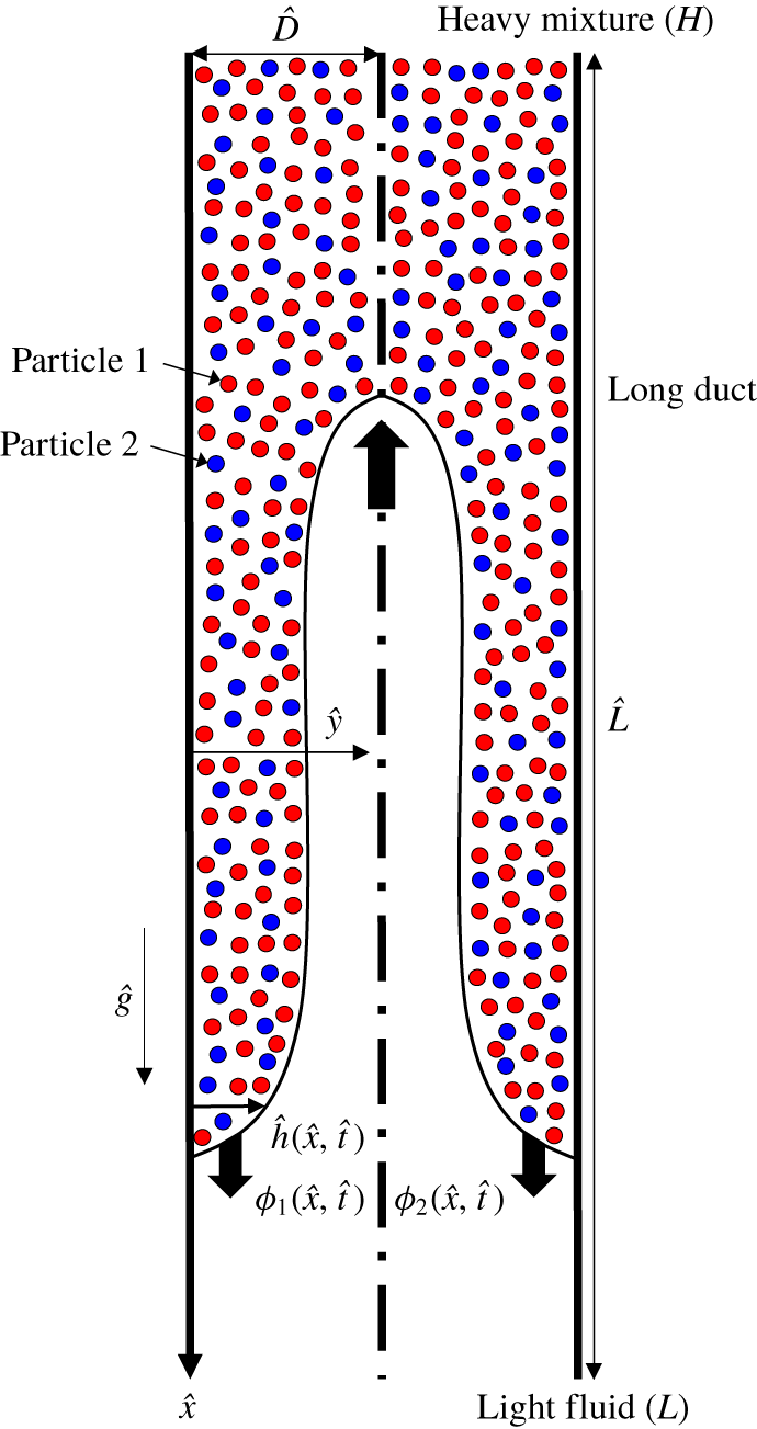
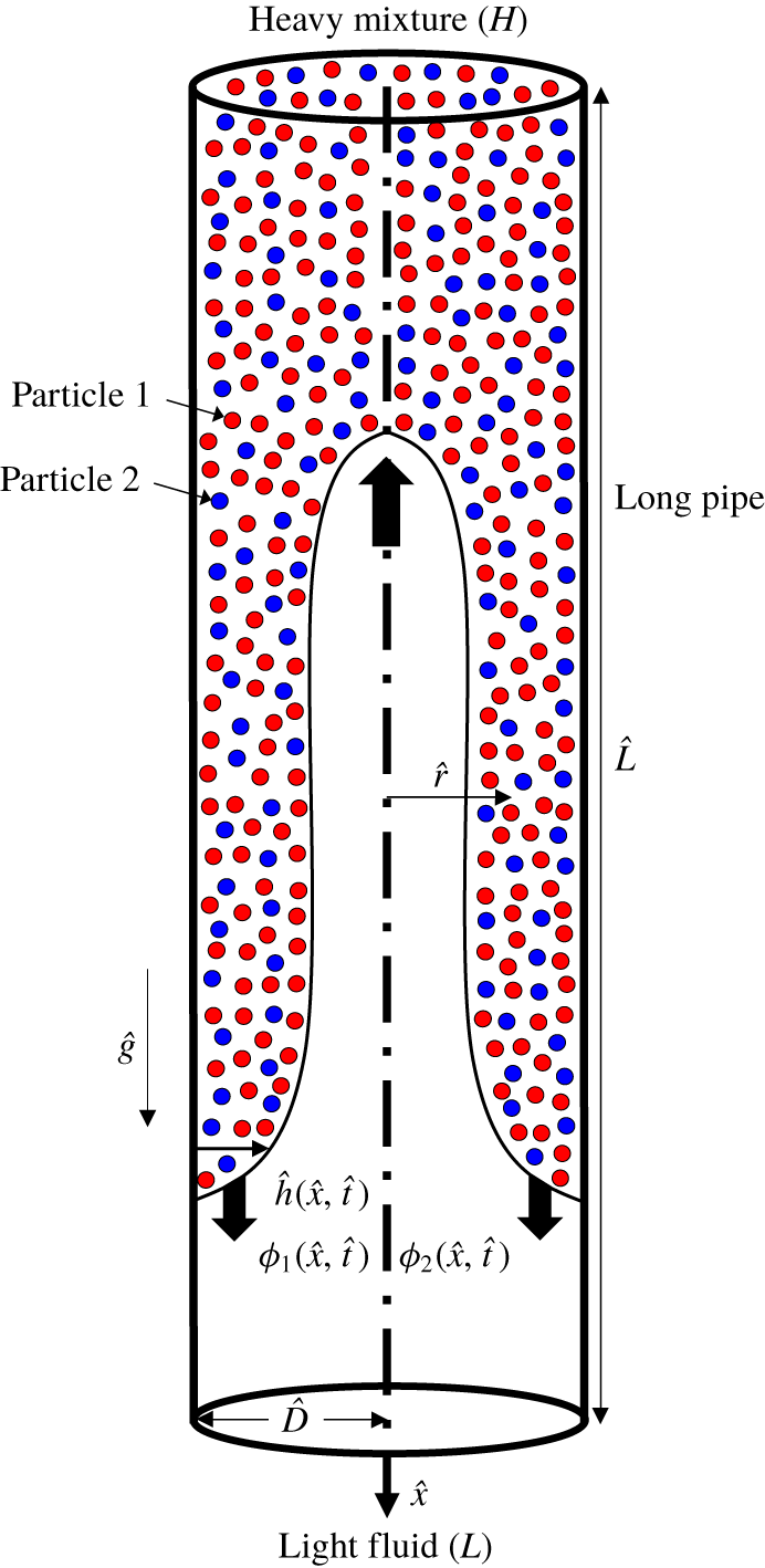
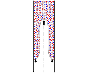
Schematic of the symmetric bidensity particle-laden exchange flow in a vertical two-dimensional duct used in the lubrication model analysis. Note that dimensional notations are used in the figure. The interface shape is illustrative only. Particle type 1 is heavier than 2 ( $\hat{\unicode[STIX]{x1D70C}}_{p,1}>\hat{\unicode[STIX]{x1D70C}}_{p,2}$).

The major novelty of the current manuscript is to extend the monodensity model of Mirzaeian & Alba (Reference Mirzaeian and Alba2018a), developed for exchange flows in a duct, to a bidensity configuration (figure 1). Such heavy–light exchange flows are widely observed in geophysical contexts as well as in plug cementing of wells. The latter process, where heavy cement slurry is released on top of the light mud to ultimately seal and abandon a well, has been mostly studied under a pure fluid and/or monodensity suspension assumption. This approach has shortcomings since various particle types are present in slurries. As explained by Cowan & Hale (Reference Cowan and Hale1994), the cement slurry or spacer fluid (used between the mud and cement) may contain different additives such as bentonite, barite, hematite or ilmenite with varying densities and possibly particle size distribution (PSD) effects (bidisperse and/or polydisperse). Note that the latter PSD factor in such cementing practices as well as other civil engineering applications is certainly of interest and to be explored in future studies. We will follow the modelling concepts given in the recent study of Wong & Bertozzi (Reference Wong and Bertozzi2016) for free-surface suspension film flows to establish the settling dynamics of bidensity suspensions. The goal is to build a robust predictive framework to fundamentally understand the dynamics of complex particle-laden flows at much lower computational cost than a fully fledged direct numerical simulation (DNS) analysis. As will be shown, the underlying governing equations and dynamics of the flow are massively altered when an additional particle phase is introduced to the problem. This occurs due to an interesting interplay between the settling velocity of the two particles. The settling velocity of particles is not simply a notion that can be generalized between monodensity, bidensity and/or polydensity cases. Each limit shall be dealt with separately using a special care, distinguishing the current study from the previous monodensity work of Mirzaeian & Alba (Reference Mirzaeian and Alba2018a). The current research will pave the way to the study of a more complicated polydensity scenario in the future, which is of particular interest in many geophysical and industrial processes. The lubrication model is first derived in § 2. The benchmarking against the monodensity limit is explained in § 3. The computed results are discussed in § 4 covering a wide range of controlling parameters such as the density, size and volume fraction of particles, as well as the viscosity and density of the light and carrying fluids and the Reynolds number. The paper closes with a brief summary in § 5.
1.1 Dimensional and dimensionless governing parameters
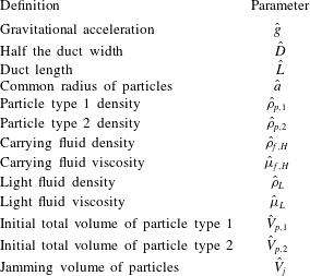
The problem shown schematically in figure 1 involves numerous dimensional parameters, which we denote with the  $\hat{~}$ symbol. The gravitational acceleration is denoted by
 ${\hat{g}}$. The vertical duct has width,
 $2\hat{D}$, and length,
 $\hat{L}$. To capture the fully developed flow effects, as discussed by Alba, Taghavi & Frigaard (Reference Alba, Taghavi and Frigaard2013a), Mirzaeian & Alba (Reference Mirzaeian and Alba2018a,Reference Mirzaeian and Albab), we assume that
 $\hat{L}\gg \hat{D}$. The solid particle types 1 and 2, which are considered to be spherical and heavier than the carrying fluid (negatively buoyant), have a common radius,
 $\hat{a}$, but different densities,
 $\hat{\unicode[STIX]{x1D70C}}_{p,1}$ and
 $\hat{\unicode[STIX]{x1D70C}}_{p,2}$ respectively. It is assumed that
 $\hat{\unicode[STIX]{x1D70C}}_{p,1}>\hat{\unicode[STIX]{x1D70C}}_{p,2}$. Non-Brownian suspension is considered in this study (
 $2\hat{a}>1~\unicode[STIX]{x03BC}\text{m}$). The Newtonian carrying fluid in the heavy solution has density
 $\hat{\unicode[STIX]{x1D70C}}_{f,H}$ and viscosity
 $\hat{\unicode[STIX]{x1D707}}_{f,H}$ and the Newtonian light fluid has density
 $\hat{\unicode[STIX]{x1D70C}}_{L}$ and viscosity
 $\hat{\unicode[STIX]{x1D707}}_{L}$. Fluids and solids are assumed to be incompressible. The initial total volume of particles is
 $\hat{V}_{p}$ and the jamming volume of particles
 $\hat{V}_{j}$. Through a dimensional analysis based on the Buckingham-
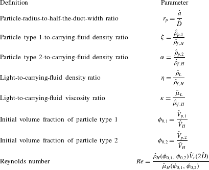
 $\unicode[STIX]{x03C0}$ theorem, it is not difficult to show that the following dimensionless parameters control the flow in question, namely the duct aspect ratio,
 $\unicode[STIX]{x1D6FF}=\hat{D}/\hat{L}\ll 1$, particle radius to half the duct width,
 $r_{p}=\hat{a}/\hat{D}$, particle type 1-to-carrying-fluid density ratio,
 $\unicode[STIX]{x1D709}=\hat{\unicode[STIX]{x1D70C}}_{p,1}/\hat{\unicode[STIX]{x1D70C}}_{f,H}$, particle type 2-to-carrying-fluid density ratio,
 $\unicode[STIX]{x1D6FC}=\hat{\unicode[STIX]{x1D70C}}_{p,2}/\hat{\unicode[STIX]{x1D70C}}_{f,H}$, light-to-carrying-fluid density ratio,
 $\unicode[STIX]{x1D702}=\hat{\unicode[STIX]{x1D70C}}_{L}/\hat{\unicode[STIX]{x1D70C}}_{f,H}$, light-to-carrying-fluid viscosity ratio,
 $\unicode[STIX]{x1D705}=\hat{\unicode[STIX]{x1D707}}_{L}/\hat{\unicode[STIX]{x1D707}}_{f,H}$, initial volume fraction of particle type 1,
 $\unicode[STIX]{x1D719}_{0,1}=\hat{V}_{p,1}/\hat{V}_{H}$, initial volume fraction of particle type 2,
 $\unicode[STIX]{x1D719}_{0,2}=\hat{V}_{p,2}/\hat{V}_{H}$, jamming volume fraction,
 $\unicode[STIX]{x1D719}_{j}=\hat{V}_{j}/\hat{V}_{H}$, and the Reynolds number,
 $Re=\hat{\unicode[STIX]{x1D70C}}_{H}(\unicode[STIX]{x1D719}_{0,1},\unicode[STIX]{x1D719}_{0,2})\hat{V}_{t}(2\hat{D})/\hat{\unicode[STIX]{x1D707}}_{H}(\unicode[STIX]{x1D719}_{0,1},\unicode[STIX]{x1D719}_{0,2})$. Given that the duct has unit depth, the total volume of the heavy solution is obtained as
 $\hat{V}_{H}=\hat{D}\hat{L}$. The jamming volume fraction is obtained as
 $\unicode[STIX]{x1D719}_{j}\approx 0.67$. The heavy fluid density is expressed as
 $\hat{\unicode[STIX]{x1D70C}}_{H}(\unicode[STIX]{x1D719}_{0,1},\unicode[STIX]{x1D719}_{0,2})=[\hat{\unicode[STIX]{x1D70C}}_{p,1}\unicode[STIX]{x1D719}_{0,1}+\hat{\unicode[STIX]{x1D70C}}_{p,2}\unicode[STIX]{x1D719}_{0,2}+\hat{\unicode[STIX]{x1D70C}}_{f,H}(1-\unicode[STIX]{x1D719}_{0,1}-\unicode[STIX]{x1D719}_{0,2})]$. The heavy fluid viscosity,
 $\hat{\unicode[STIX]{x1D707}}_{H}(\unicode[STIX]{x1D719}_{0,1},\unicode[STIX]{x1D719}_{0,2})$, will be explained in the next section. The characteristic velocity in the Reynolds-number expression is defined as
 $\hat{V}_{t}=\sqrt{(1-\unicode[STIX]{x1D713}){\hat{g}}\hat{D}/(1+\unicode[STIX]{x1D713})}$ with
 $\unicode[STIX]{x1D713}=\hat{\unicode[STIX]{x1D70C}}_{L}/\hat{\unicode[STIX]{x1D70C}}_{H}(\unicode[STIX]{x1D719}_{0,1},\unicode[STIX]{x1D719}_{0,2})=\unicode[STIX]{x1D702}/(1+(\unicode[STIX]{x1D709}-1)\unicode[STIX]{x1D719}_{0,1}+(\unicode[STIX]{x1D6FC}-1)\unicode[STIX]{x1D719}_{0,2})$ being the ratio of the density of the light fluid to the heavy suspension. In our simulations,
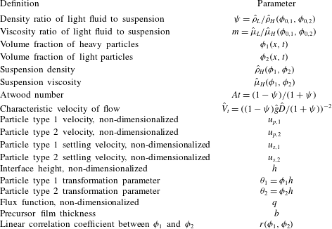
 $\unicode[STIX]{x1D713}$ is always less than one, meaning that the overall suspension fluid is heavier than the light fluid. The dimensional and dimensionless parameters governing the flow are listed in tables 1 and 2. Table 3 summarizes a list of the remaining secondary parameters that are conveniently used throughout this article.
List of dimensional independent input parameters of the problem.

List of dimensionless independent input parameters of the problem. Note that the study is conducted in the small aspect ratio limit ( $\unicode[STIX]{x1D6FF}=\hat{D}/\hat{L}\ll 1$) and a jamming volume fraction of
 $\unicode[STIX]{x1D719}_{j}\approx 0.67$.

List of secondary parameters of the problem.

1.2 Underlying assumptions and limitations
(I) At time  $\hat{t}=0~\text{s}$ the heavy suspension occupies the top half of the duct (
 $\hat{x}<0$) and the light pure fluid takes the bottom half (
 $\hat{x}\geqslant 0$); see figure 1. The duct is assumed to be sufficiently long (
 $\unicode[STIX]{x1D6FF}\ll 1$) such that no end effects are introduced. In this study, we focused on the frontal and interface region between the heavy and light fluids. The assumption of a sufficiently long duct corresponds to a continuous supply of particles to the finite-length frontal and interface region through the settling process. (II) We assume a small density difference between the suspension phase and the pure fluid. As discussed in depth in appendix A, for a particular Boussinesq limit considered (
 $At\ll \unicode[STIX]{x1D6FF}\ll 1$, where
 $At=(\hat{\unicode[STIX]{x1D70C}}_{H}(\unicode[STIX]{x1D719}_{0,1},\unicode[STIX]{x1D719}_{0,2})-\hat{\unicode[STIX]{x1D70C}}_{L})/(\hat{\unicode[STIX]{x1D70C}}_{H}(\unicode[STIX]{x1D719}_{0,1},\unicode[STIX]{x1D719}_{0,2})+\hat{\unicode[STIX]{x1D70C}}_{L})=(1-\unicode[STIX]{x1D713})/(1+\unicode[STIX]{x1D713})$ is the Atwood number), we may neglect the diffusive effects associated with shear-induced migration of particles; see also Mirzaeian & Alba (Reference Mirzaeian and Alba2018a). This will, in turn, result in a uniform volume fraction of particles across the depth of the suspension layer,
 $y$, i.e.
 $\unicode[STIX]{x1D719}_{1}=\unicode[STIX]{x1D719}_{1}(x,t)$ and
 $\unicode[STIX]{x1D719}_{2}=\unicode[STIX]{x1D719}_{2}(x,t)$ only. This assumption is consistent with that made in our monodensity study. (III) We further neglect the effects of an interfacial tension between the two fluids for simplicity. In other words, we consider an immiscible interface but with zero interfacial tension. Such a limit is indeed equivalent to a miscible interface with zero molecular diffusion; see Taghavi et al. (Reference Taghavi, Alba, Seon, Wielage-Burchard, Martinez and Frigaard2012) and Alba, Taghavi & Frigaard (Reference Alba, Taghavi and Frigaard2013b) for studies taking a similar approach for pure fluids and Mirzaeian & Alba (Reference Mirzaeian and Alba2018a) for monodensity suspensions. Such an assumption is relevant to a range of cementing operations utilizing a water-based mud. Refer to Hasnain, Segura & Alba (Reference Hasnain, Segura and Alba2017) for exchange flow of immiscible fluids with applications in cementing of wells drilled using an oil-based mud. The present study is limited to laminar flows with stable interfaces between the two fluids i.e. in the absence of interfacial instabilities. (IV) Even though the particle phases in this study may assume different densities, their sizes are the same. Since the viscosity of a suspension is known to be related only to the particle geometry rather than density, we can approximate the viscosity of the bidensity suspension as that of a monodisperse case (Krieger–Dougherty relation),
 $\hat{\unicode[STIX]{x1D707}}_{H}(\unicode[STIX]{x1D719}_{0,1},\unicode[STIX]{x1D719}_{0,2})=\hat{\unicode[STIX]{x1D707}}_{f,H}[1-(\unicode[STIX]{x1D719}_{0,1}+\unicode[STIX]{x1D719}_{0,2})/\unicode[STIX]{x1D719}_{j}]^{-2}$. The computational program would fail if the particle volume fraction in the enriched areas reached the jamming volume fraction (
 $\hat{\unicode[STIX]{x1D707}}_{f,H}\rightarrow \infty$ as
 $(\unicode[STIX]{x1D719}_{0,1}+\unicode[STIX]{x1D719}_{0,2})\rightarrow \unicode[STIX]{x1D719}_{j}$).
2 Lubrication model derivation
We aim to develop a lubrication model in simplified vertical two-dimensional (2-D) channel geometry shown schematically in figure 1. Only half of the duct domain is considered in the model due to the symmetry ( $0\leqslant y\leqslant 1$). Lubrication model for a pipe geometry, potentially more convenient for future experimentation, is provided in appendix B. Following the recent approach of Mirzaeian & Alba (Reference Mirzaeian and Alba2018a) for monodensity exchange flows, the governing streamwise and depthwise momentum equations in the heavy particle-laden layer reduce to
 $$\begin{eqnarray}\displaystyle & \displaystyle 0=-p_{x}+\frac{\unicode[STIX]{x1D70C}_{H}(\unicode[STIX]{x1D719}_{1},\unicode[STIX]{x1D719}_{2})Re}{1-\unicode[STIX]{x1D713}}+\unicode[STIX]{x1D707}_{H}(\unicode[STIX]{x1D719}_{1},\unicode[STIX]{x1D719}_{2})u_{yy}, & \displaystyle\end{eqnarray}$$
 $$\begin{eqnarray}\displaystyle & \displaystyle 0=-p_{y}, & \displaystyle\end{eqnarray}$$
where the streamwise and depthwise distances are scaled by  $\hat{D}/\unicode[STIX]{x1D6FF}$ and
 $\hat{D}$ respectively. Moreover, the pressure is scaled by
 $\hat{\unicode[STIX]{x1D707}}_{H}(\unicode[STIX]{x1D719}_{0,1},\unicode[STIX]{x1D719}_{0,2})\hat{V}_{t}/(\unicode[STIX]{x1D6FF}\hat{D})$. The dimensionless density and viscosity of the heavy layer in continuum form and as a function of the particle volume fraction,
 $\unicode[STIX]{x1D719}_{1}$ and
 $\unicode[STIX]{x1D719}_{2}$, are expressed below, see Wong & Bertozzi (Reference Wong and Bertozzi2016),
 $$\begin{eqnarray}\displaystyle & \displaystyle \unicode[STIX]{x1D70C}_{H}(\unicode[STIX]{x1D719}_{1},\unicode[STIX]{x1D719}_{2})=\frac{1+(\unicode[STIX]{x1D709}-1)\unicode[STIX]{x1D719}_{1}+(\unicode[STIX]{x1D6FC}-1)\unicode[STIX]{x1D719}_{2}}{1+(\unicode[STIX]{x1D709}-1)\unicode[STIX]{x1D719}_{0,1}+(\unicode[STIX]{x1D6FC}-1)\unicode[STIX]{x1D719}_{0,2}}, & \displaystyle\end{eqnarray}$$
 $$\begin{eqnarray}\displaystyle & \displaystyle \unicode[STIX]{x1D707}_{H}(\unicode[STIX]{x1D719}_{1},\unicode[STIX]{x1D719}_{2})=\frac{[1-(\unicode[STIX]{x1D719}_{1}+\unicode[STIX]{x1D719}_{2})/\unicode[STIX]{x1D719}_{j}]^{-2}}{[1-(\unicode[STIX]{x1D719}_{0,1}+\unicode[STIX]{x1D719}_{0,2})/\unicode[STIX]{x1D719}_{j}]^{-2}}. & \displaystyle\end{eqnarray}$$
Similarly, for the light fluid layer we may obtain
 $$\begin{eqnarray}\displaystyle & \displaystyle 0=-p_{x}+\frac{\unicode[STIX]{x1D713}Re}{1-\unicode[STIX]{x1D713}}+mu_{yy}, & \displaystyle\end{eqnarray}$$
 $$\begin{eqnarray}\displaystyle & \displaystyle 0=-p_{y}, & \displaystyle\end{eqnarray}$$
with  $m=\hat{\unicode[STIX]{x1D707}}_{L}/\hat{\unicode[STIX]{x1D707}}_{H}(\unicode[STIX]{x1D719}_{0,1},\unicode[STIX]{x1D719}_{0,2})=\unicode[STIX]{x1D705}[1-(\unicode[STIX]{x1D719}_{0,1}+\unicode[STIX]{x1D719}_{0,2})/\unicode[STIX]{x1D719}_{j}]^{2}$ being the viscosity ratio of the light fluid to that of the heavy suspension layer. Integrating (2.2) and (2.6) across the width gives
 $$\begin{eqnarray}p=p_{0}(x,t)+\frac{\unicode[STIX]{x1D70C}_{H}(\unicode[STIX]{x1D719}_{1},\unicode[STIX]{x1D719}_{2})xRe}{1-\unicode[STIX]{x1D713}},\quad 0\leqslant y\leqslant 1,\end{eqnarray}$$
where  $p_{0}(x,t)$ is defined as
 $$\begin{eqnarray}p_{0}(x,t)=p(x,0,t)-\frac{\unicode[STIX]{x1D70C}_{H}(\unicode[STIX]{x1D719}_{1},\unicode[STIX]{x1D719}_{2})xRe}{1-\unicode[STIX]{x1D713}}.\end{eqnarray}$$
The pressure expression (2.7) is then used in the streamwise momentum equations (2.1) and (2.5) to give
 $$\begin{eqnarray}\displaystyle & \displaystyle 0=-P_{0,x}+\unicode[STIX]{x1D707}_{H}(\unicode[STIX]{x1D719}_{1},\unicode[STIX]{x1D719}_{2})u_{yy},\quad 0\leqslant y\leqslant h, & \displaystyle\end{eqnarray}$$
 $$\begin{eqnarray}\displaystyle & \displaystyle 0=-P_{0,x}-\frac{\unicode[STIX]{x1D70C}_{H}(\unicode[STIX]{x1D719}_{1},\unicode[STIX]{x1D719}_{2})-\unicode[STIX]{x1D713}}{1-\unicode[STIX]{x1D713}}Re+mu_{yy},\quad h\leqslant y\leqslant 1. & \displaystyle\end{eqnarray}$$
Note that, for simplicity, we have defined  $P_{0,x}=p_{0,x}+(x\unicode[STIX]{x1D70C}_{H,x}Re)/(1-\unicode[STIX]{x1D713})$. A narrow precursor suspension film of thickness
 $b$ is assumed in the vicinity of the wall. The no-slip boundary condition can be routinely applied at the wall i.e.
 $y=0$. Other boundary conditions are the stress-free condition in the duct centre (
 $y=1$) due to the symmetry and the homogeneity of the velocity and stress at the interface (
 $y=h$). The last condition needed to solve the system of (2.9) and (2.10), rectifying velocity closures, is the total flow constraint.
The streamwise velocity,  $u$, in the heavy and light layers can then be obtained by integrating (2.9) and (2.10) twice as
 $$\begin{eqnarray}\displaystyle & \displaystyle u=\frac{P_{0,x}y^{2}}{2\unicode[STIX]{x1D707}_{H}}+c_{1}y+c_{2},\quad 0\leqslant y\leqslant h, & \displaystyle\end{eqnarray}$$
 $$\begin{eqnarray}\displaystyle & \displaystyle u=\left(P_{0,x}+\frac{\unicode[STIX]{x1D70C}_{H}-\unicode[STIX]{x1D713}}{1-\unicode[STIX]{x1D713}}Re\right)\frac{y^{2}}{2m}+d_{1}y+d_{2},\quad h\leqslant y\leqslant 1, & \displaystyle\end{eqnarray}$$
with  $P_{0,x}$,
 $c_{1}$,
 $c_{2}$,
 $d_{1}$ and
 $d_{2}$ as coefficients given in appendix C. The flux function,
 $q=\hat{q}/\hat{D}$, rendering the flow rate within the heavy layer can eventually be calculated as
 $$\begin{eqnarray}q=\int _{0}^{h}u\,\text{d}y,\end{eqnarray}$$
which is given in appendix D in terms of  $h$,
 $Re$,
 $\unicode[STIX]{x1D705}$,
 $\unicode[STIX]{x1D707}_{H}$ and
 $\unicode[STIX]{x1D70C}_{H}$. Note that the flux function,
 $q$, for the bidensity case is similar to the monodensity one given by Mirzaeian & Alba (Reference Mirzaeian and Alba2018a), except that the
 $\unicode[STIX]{x1D707}_{H}$ and
 $\unicode[STIX]{x1D70C}_{H}$ expressions used are different.
The evolution equations for the interface height and volume fraction of particle types 1 and 2 respectively read, see also Wong (Reference Wong2017),
 $$\begin{eqnarray}\displaystyle & h_{t}+q_{x}=0, & \displaystyle\end{eqnarray}$$
 $$\begin{eqnarray}\displaystyle & (\unicode[STIX]{x1D719}_{1}h)_{t}+(u_{p,1}\unicode[STIX]{x1D719}_{1}h)_{x}=0, & \displaystyle\end{eqnarray}$$
 $$\begin{eqnarray}\displaystyle & (\unicode[STIX]{x1D719}_{2}h)_{t}+(u_{p,2}\unicode[STIX]{x1D719}_{2}h)_{x}=0, & \displaystyle\end{eqnarray}$$
where  $u_{p,1}$ and
 $u_{p,2}$ are the particle velocities expressible as
 $$\begin{eqnarray}\displaystyle & \displaystyle u_{p,1}=\frac{q}{h}+(1-\unicode[STIX]{x1D719}_{1})u_{s,1}-\unicode[STIX]{x1D719}_{2}u_{s,2}, & \displaystyle\end{eqnarray}$$
 $$\begin{eqnarray}\displaystyle & \displaystyle u_{p,2}=\frac{q}{h}-\unicode[STIX]{x1D719}_{1}u_{s,1}+(1-\unicode[STIX]{x1D719}_{2})u_{s,2}. & \displaystyle\end{eqnarray}$$
Here,  $u_{s,1}$ and
 $u_{s,2}$ are the dimensionless hindered Stokes settling velocities of particle types 1 and 2 respectively. In (2.14)–(2.16), time is scaled by
 $\hat{D}/(\unicode[STIX]{x1D6FF}\hat{V}_{t})$. According to Revay & Higdon (Reference Revay and Higdon1992), Tripathi & Acrivos (Reference Tripathi and Acrivos1999) and Wong & Bertozzi (Reference Wong and Bertozzi2016), for bidensity suspensions we have
 $$\begin{eqnarray}u_{s,i}=\frac{2\hat{a}^{2}{\hat{g}}w(h)}{9\hat{V}_{t}\hat{\unicode[STIX]{x1D707}}_{f,H}}\left[M_{o}(\hat{\unicode[STIX]{x1D70C}}_{p,i}-\hat{\unicode[STIX]{x1D70C}}_{f,H})+M_{I}\mathop{\sum }_{k=1}^{2}(\hat{\unicode[STIX]{x1D70C}}_{p,k}-\hat{\unicode[STIX]{x1D70C}}_{f,H})\frac{\unicode[STIX]{x1D719}_{k}}{\unicode[STIX]{x1D719}_{1}+\unicode[STIX]{x1D719}_{2}}\right],\quad i=1,2,\end{eqnarray}$$
where  $M_{o}=1-(\unicode[STIX]{x1D719}_{1}+\unicode[STIX]{x1D719}_{2})/\unicode[STIX]{x1D719}_{j}$ is the self-mobility and
 $M_{I}=[1-(\unicode[STIX]{x1D719}_{1}+\unicode[STIX]{x1D719}_{2})][1-(\unicode[STIX]{x1D719}_{1}+\unicode[STIX]{x1D719}_{2})/\unicode[STIX]{x1D719}_{j}]^{2}-M_{o}$ is the interaction mobility. Moreover,
 $w(h)$ is the wall function chosen as
 $w(h)=h^{2}$ to give 0 and 1 at the wall (
 $h=0$) and centre (
 $h=1$) respectively; see also Mirzaeian & Alba (Reference Mirzaeian and Alba2018a). It is not difficult to write (2.19) in non-dimensional form as
 $$\begin{eqnarray}\displaystyle & \displaystyle u_{s,1}=\frac{\unicode[STIX]{x1D713}\unicode[STIX]{x1D705}Re(1+\unicode[STIX]{x1D713})r_{p}^{2}w(h)}{9m\unicode[STIX]{x1D702}(1-\unicode[STIX]{x1D713})}\left[M_{o}(\unicode[STIX]{x1D709}-1)+M_{I}\frac{(\unicode[STIX]{x1D709}-1)\unicode[STIX]{x1D719}_{1}+(\unicode[STIX]{x1D6FC}-1)\unicode[STIX]{x1D719}_{2}}{\unicode[STIX]{x1D719}_{1}+\unicode[STIX]{x1D719}_{2}}\right], & \displaystyle\end{eqnarray}$$
 $$\begin{eqnarray}\displaystyle & \displaystyle u_{s,2}=\frac{\unicode[STIX]{x1D713}\unicode[STIX]{x1D705}Re(1+\unicode[STIX]{x1D713})r_{p}^{2}w(h)}{9m\unicode[STIX]{x1D702}(1-\unicode[STIX]{x1D713})}\left[M_{o}(\unicode[STIX]{x1D6FC}-1)+M_{I}\frac{(\unicode[STIX]{x1D709}-1)\unicode[STIX]{x1D719}_{1}+(\unicode[STIX]{x1D6FC}-1)\unicode[STIX]{x1D719}_{2}}{\unicode[STIX]{x1D719}_{1}+\unicode[STIX]{x1D719}_{2}}\right]. & \displaystyle\end{eqnarray}$$
In order to advantageously solve the system of equations (2.14)–(2.16) in a conservative framework, we define additional parameters as  $\unicode[STIX]{x1D703}_{1}=\unicode[STIX]{x1D719}_{1}h$, and
 $\unicode[STIX]{x1D703}_{2}=\unicode[STIX]{x1D719}_{2}h$. Plugging these variables into (2.14)–(2.16) results in the following set of equations, simply in the form of a classical Riemann problem:
 $$\begin{eqnarray}\displaystyle & h_{t}+F_{x}(h,\unicode[STIX]{x1D703}_{1},\unicode[STIX]{x1D703}_{2})=0, & \displaystyle\end{eqnarray}$$
 $$\begin{eqnarray}\displaystyle & \unicode[STIX]{x1D703}_{1,t}+G_{x}(h,\unicode[STIX]{x1D703}_{1},\unicode[STIX]{x1D703}_{2})=0, & \displaystyle\end{eqnarray}$$
 $$\begin{eqnarray}\displaystyle & \unicode[STIX]{x1D703}_{2,t}+Z_{x}(h,\unicode[STIX]{x1D703}_{1},\unicode[STIX]{x1D703}_{2})=0, & \displaystyle\end{eqnarray}$$
where
 $$\begin{eqnarray}\displaystyle & F(h,\unicode[STIX]{x1D703}_{1},\unicode[STIX]{x1D703}_{2})=q(h,\unicode[STIX]{x1D703}_{1},\unicode[STIX]{x1D703}_{2}), & \displaystyle\end{eqnarray}$$
 $$\begin{eqnarray}\displaystyle & G(h,\unicode[STIX]{x1D703}_{1},\unicode[STIX]{x1D703}_{2})=u_{p,1}(h,\unicode[STIX]{x1D703}_{1},\unicode[STIX]{x1D703}_{2})\unicode[STIX]{x1D703}_{1}, & \displaystyle\end{eqnarray}$$
 $$\begin{eqnarray}\displaystyle & Z(h,\unicode[STIX]{x1D703}_{1},\unicode[STIX]{x1D703}_{2})=u_{p,2}(h,\unicode[STIX]{x1D703}_{1},\unicode[STIX]{x1D703}_{2})\unicode[STIX]{x1D703}_{2}. & \displaystyle\end{eqnarray}$$
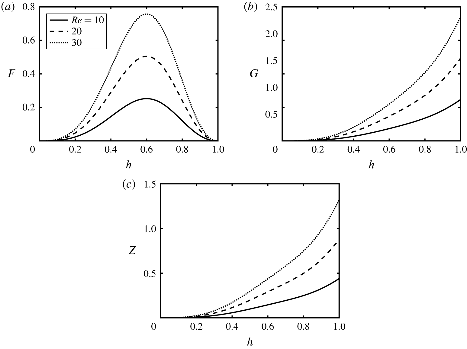
The kinematic conditions (2.22)–(2.24) along with the total flow constraint condition ensures conservation of pure fluid as well as particle total mass, and thus the volume and area due to the presumed incompressibility, at all times. Figure 2(a–c) shows the variation of the  $F$,
 $G$ and
 $Z$ functions, respectively, versus
 $h$ for different values of
 $Re$. As
 $h\rightarrow 0$, all
 $F,G,Z\rightarrow 0$;
 $F$ exhibits a maximum in the interval
 $h\in [0,1]$. In the iso-viscous case,
 $\unicode[STIX]{x1D705}=1$, the location of this maximum remains unchanged (
 $h\approx 0.6$), which can shift with viscosity ratio. Magnitude of the function
 $G$ governing the evolution of particle type 1 is larger than that of function
 $Z$ controlling particle type 2 motion due to the choice of densities (
 $\unicode[STIX]{x1D709}=1.9$ versus
 $\unicode[STIX]{x1D6FC}=1.45$ in figure 2). The final takeaway from figure 2 is that all the flux function values,
 $F$,
 $G$ and
 $Z$ increase with the Reynolds number,
 $Re$, which can also be verified from (2.25)–(2.27) and flux function,
 $q$, given in appendix D. Our methodology to numerically solve the system of partial differential equations (PDE) (2.22)–(2.24) in space,
 $x$, and time,
 $t$, is based on the robust explicit high-resolution TVD finite difference scheme explained in Mirzaeian & Alba (Reference Mirzaeian and Alba2018a), thus, is not presented here for brevity. We have carefully upgraded our code to accommodate an added PDE (2.27). It has been successfully tested on the relevant works of Kurganov & Tadmor (Reference Kurganov and Tadmor2000), Hasnain & Alba (Reference Hasnain and Alba2017) and Cook et al. (Reference Cook, Bertozzi and Hosoi2008).
Variation of the flux functions (a)  $F$, (b)
 $G$ and (c)
 $Z$ in (2.25)–(2.27) with interface height,
 $h$ at various values of
 $Re$. Other parameters used are
 $\unicode[STIX]{x1D719}_{0,1}=\unicode[STIX]{x1D719}_{0,2}=0.2$,
 $\unicode[STIX]{x1D705}=1$,
 $r_{p}=0.06$,
 $\unicode[STIX]{x1D709}=1.9$,
 $\unicode[STIX]{x1D6FC}=1.45$ and
 $\unicode[STIX]{x1D702}=1.25$.

3 Benchmarking against the monodensity limit
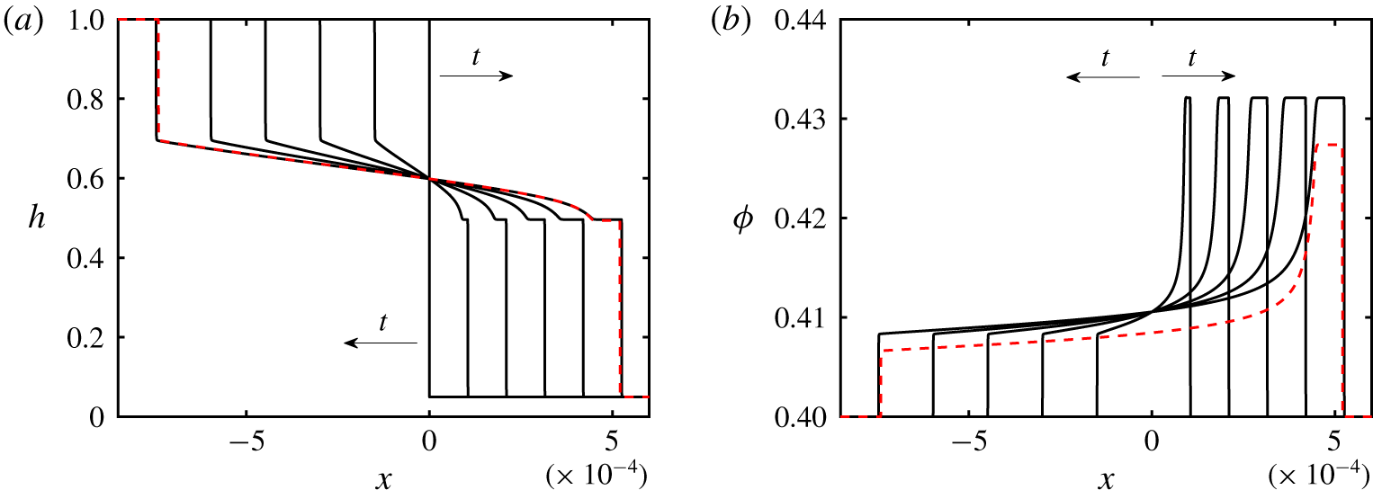
Evolution of the (a) interface height,  $h$, and (b) particle volume fraction,
 $\unicode[STIX]{x1D719}$, with time,
 $t=[0,0.02,0.04,\ldots ,0.1]$. The parameters used are
 $Re=0.1$,
 $\unicode[STIX]{x1D705}=1$,
 $r_{p}=0.06$,
 $\unicode[STIX]{x1D709}=1.9$,
 $\unicode[STIX]{x1D702}=1.25$,
 $\unicode[STIX]{x1D719}_{0,1}=0.4$,
 $\unicode[STIX]{x1D719}_{0,2}=0$ and
 $\unicode[STIX]{x1D6FC}=1.9$. The red dashed lines show the predictions of the monodensity model of Mirzaeian & Alba (Reference Mirzaeian and Alba2018a) at
 $t=0.1$.

Setting  $\unicode[STIX]{x1D719}_{0,2}=0$ in the bidensity model (2.14)–(2.16) should, in theory, result in a monodensity system. Monodensity exchange flows are studied in detail in Mirzaeian & Alba (Reference Mirzaeian and Alba2018a). We aim to find out how the two models compare in this limit. Figure 3(a) shows the evolution of the interface height profile with time,
 $t$, obtained for
 $\unicode[STIX]{x1D719}_{0,1}=0.4$,
 $\unicode[STIX]{x1D719}_{0,2}=0$,
 $Re=0.1$,
 $\unicode[STIX]{x1D705}=1$,
 $r_{p}=0.06$,
 $\unicode[STIX]{x1D709}=1.9$ and
 $\unicode[STIX]{x1D702}=1.25$. The precursor height is chosen to be
 $b=0.05$ in all presented simulations unless otherwise stated. Note that the chosen precursor value, which is still much smaller than the range typically used in thin film flow studies e.g. Spaid & Homsy (Reference Spaid and Homsy1996), is slightly larger than that used in our monodensity study (
 $b=0.01$). This adjustment has been carried out in order to overcome certain numerical issues associated with the formation of singular shocks in the bidensity case. The interface height is initially
 $h=1$ and 0 over
 $x<0$ and
 $x\geqslant \text{d}x$ respectively, i.e. the heavy (light) fluid occupying the left (right) side of the duct. There is no sensitivity of the solution to the choice of initial condition, as discussed by Mirzaeian & Alba (Reference Mirzaeian and Alba2018a). The output of the monodensity model of Mirzaeian & Alba (Reference Mirzaeian and Alba2018a) at
 $t=0.1$ is added to figure 3, showing some degree of deviation with that of the bidensity model (current study). The difference is due to the fact that the particle slip velocity in the monodensity case is given as
 $$\begin{eqnarray}u_{s}=f(\unicode[STIX]{x1D719})w(h)\frac{\unicode[STIX]{x1D713}\unicode[STIX]{x1D705}Re(1+\unicode[STIX]{x1D713})r_{p}^{2}(\unicode[STIX]{x1D709}-1)}{9m\unicode[STIX]{x1D702}(1-\unicode[STIX]{x1D713})},\end{eqnarray}$$
where  $f(\unicode[STIX]{x1D719})=(1-\unicode[STIX]{x1D719})^{5}$ is the Richardson–Zaki settling function. However, on the other hand, setting
 $\unicode[STIX]{x1D719}_{2}=0$ in the bidensity slip velocity formula (2.20) will result in
 $$\begin{eqnarray}u_{s}=(1-\unicode[STIX]{x1D719})\left(1-\frac{\unicode[STIX]{x1D719}}{\unicode[STIX]{x1D719}_{j}}\right)^{2}w(h)\frac{\unicode[STIX]{x1D713}\unicode[STIX]{x1D705}Re(1+\unicode[STIX]{x1D713})r_{p}^{2}(\unicode[STIX]{x1D709}-1)}{9m\unicode[STIX]{x1D702}(1-\unicode[STIX]{x1D713})},\end{eqnarray}$$
which is different from (3.1). Note how these two velocity expressions differ solely over their ‘hinderance multiplier’,  $f(\unicode[STIX]{x1D719})$, thus the results might show a dependence on the choice of
 $f$. The hinderance multiplier can indeed become an important issue at high particle fractions, emphasizing the limitation on the range of validity between the monodensity and bidensity models. There are several other functions that could be considered for the slip velocity in either the monodensity or bidensity formulation with adequate confidence; regardless, we can still appreciate a clear qualitative agreement between the two studies. The profiles of volume fraction,
 $\unicode[STIX]{x1D719}=\unicode[STIX]{x1D719}_{1}$, are shown in figure 3(b). The accumulation of particles (enrichment) due to settling close to the heavy layer frontal region is evident; see Mirzaeian & Alba (Reference Mirzaeian and Alba2018a) for details. We have also confirmed the same results by switching the volume fractions, i.e. setting
 $\unicode[STIX]{x1D719}_{0,1}=0$ and
 $\unicode[STIX]{x1D719}_{0,2}=0.4$ instead of
 $\unicode[STIX]{x1D719}_{0,1}=0.4$ and
 $\unicode[STIX]{x1D719}_{0,2}=0$, which revealed that the model rightly holds symmetry with respect to particle types 1 and 2 (results not presented here for brevity). We emphasize that the formation of shock-type features, such as those demonstrated in figure 3, is not uncommon in gravity currents as discussed by Seon et al. (Reference Seon, Hulin, Salin, Perrin and Hinch2004) and Hasnain et al. (Reference Hasnain, Segura and Alba2017). We do, however, acknowledge that there may not be a one-to-one matching between the lubrication model and the real-world situation due to the underlying simplifications made in the former.
4 Results
4.1 Enrichment–depletion transition
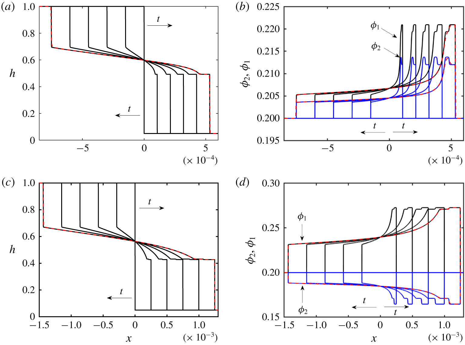
Evolution of the (a) interface height,  $h$, and (b) particle volume fraction,
 $\unicode[STIX]{x1D719}_{1}$ (black line) and
 $\unicode[STIX]{x1D719}_{2}$ (blue line), with time,
 $t=[0,0.02,0.04,\ldots ,0.1]$. The parameters used are
 $Re=0.1$,
 $\unicode[STIX]{x1D705}=1$,
 $r_{p}=0.06$,
 $\unicode[STIX]{x1D709}=1.9$,
 $\unicode[STIX]{x1D702}=1.25$,
 $\unicode[STIX]{x1D719}_{0,1}=\unicode[STIX]{x1D719}_{0,2}=0.2$ and
 $\unicode[STIX]{x1D6FC}=1.85$. (c,d) The same as (a) and (b) except they are for results obtained for
 $\unicode[STIX]{x1D6FC}=1.45$. The red dashed lines show the solution at
 $t=0.1$ for
 $\text{d}x=2\times 10^{-6}$ which is almost indistinguishable from that of
 $\text{d}x=2\times 10^{-7}$.

We now examine the bidensity particle-laden exchange flows. The initial volume fraction of particles in figure 3 was chosen to be  $\unicode[STIX]{x1D719}_{0}=0.4$. We would like to examine how the dynamics of the flow is altered if such a total volume fraction is partly created by two particles of different density. Figures 4(a) and 4(c) depict the evolution of the interface height,
 $h$, with time,
 $t$ and streamwise distance,
 $x$, obtained for
 $\unicode[STIX]{x1D719}_{0,1}=\unicode[STIX]{x1D719}_{0,2}=0.2$ and
 $\unicode[STIX]{x1D6FC}=1.85$ and 1.45 respectively. The rest of the parameters used are the same as figure 3 (
 $Re=0.1$,
 $\unicode[STIX]{x1D705}=1$,
 $r_{p}=0.06$,
 $\unicode[STIX]{x1D709}=1.9$ and
 $\unicode[STIX]{x1D702}=1.25$). The computed solutions for
 $\text{d}x=2\times 10^{-6}$ at
 $t=0.1$ are added to the figure,showing full convergence to
 $\text{d}x=2\times 10^{-7}$ i.e. results are independent of the mesh size. The ridged zone close to the heavy suspension front is more heightened in case (a) compared to (c). The corresponding volume fraction profiles,
 $\unicode[STIX]{x1D719}_{1}$ and
 $\unicode[STIX]{x1D719}_{2}$, to figures 4(a) and 4(c) are given in panels (b) and (d) respectively. Particle type 1 and 2 volume fractions,
 $\unicode[STIX]{x1D719}_{1}$ and
 $\unicode[STIX]{x1D719}_{2}$, are distinguished by arrows as well as black and blue lines respectively here and in the remainder of the paper. We can observe two scenarios: figure 4(b) indicates enrichment of both particle types 1 and 2 compared to the base level (
 $\unicode[STIX]{x1D719}_{0,1}=\unicode[STIX]{x1D719}_{0,2}=0.2$) along the interface between the two fluids. In this case, the density of particle type 2 is only slightly less than that of 1 (
 $\unicode[STIX]{x1D709}=1.9$ and
 $\unicode[STIX]{x1D6FC}=1.85$). An increase in
 $\unicode[STIX]{x1D719}_{1}$ (heavier particle) is more pronounced than
 $\unicode[STIX]{x1D719}_{2}$ (lighter particle), especially in the vicinity of the advancing heavy front. However, figure 4(d) interestingly demonstrates that, when the density of particle type 2 is noticeably less than that of particle type 1 (
 $\unicode[STIX]{x1D709}=1.9$ and
 $\unicode[STIX]{x1D6FC}=1.45$), there can occur enrichment in
 $\unicode[STIX]{x1D719}_{1}$ but depletion in
 $\unicode[STIX]{x1D719}_{2}$! Since we frequently need to use
 $\unicode[STIX]{x1D6FC}=1.85$ and 1.45 values in the remaining simulations in this paper, we will refer to the flows corresponding to the former and latter conditions as the enrichment and depletion cases, respectively.
A question that arises is whether particles cross the interface between the fluids as they accumulate near the front. Due to model constraints as well as other physical effects, the answer is perhaps no. Particles tend to slow down as they approach the concentrated area near the front. This effect may be properly inferred by understanding the viscosity–concentration relation in the suspension, i.e. more particles result in a higher viscosity and thus a slower flow. To avoid stagnation at the contact line (equivalent to a singularity in the computational model), the ridged front gradually elongates between two chasing shocks (figure 4b). Now, more volume becomes available for particles arriving at the front from the bulk of the suspension. As the extent of the enriched domain is stretched, the viscosity is also regulated in the area to ensure flow continuation. This effect is reminiscent of the Rankine–Hugoniot shock condition in a suspension flow, which was proven both theoretically and experimentally by Zhou et al. (Reference Zhou, Dupuy, Bertozzi and Hosoi2005). In line with the Rankine–Hugoniot shock condition, also found are a pair of shock-type perturbations propagating with mismatched speeds (faster frontrunner, slower tailgater), constantly adjusting the local viscosity and stabilizing the particle distribution along the interface (figure 4). Therefore, wherever particles go, the interface will also deform such that particles may stay within the suspension. Lubrication models developed for suspension flow have been solved numerically by Zhou et al. (Reference Zhou, Dupuy, Bertozzi and Hosoi2005) and Cook (Reference Cook2007) with and without surface tension. Only a minor change in shape of the interface (capillary ridge) is observed when surface tension is included in the model. The enrichment level of the particles as well as the overall shape of the interface with and without surface tension follow closely those of experiment e.g. shown by Zhou et al. (Reference Zhou, Dupuy, Bertozzi and Hosoi2005). This further signifies the fact that the particles may stay bounded within the suspension phase regardless of the surface tension, which requires future experimentation in the bidensity case.
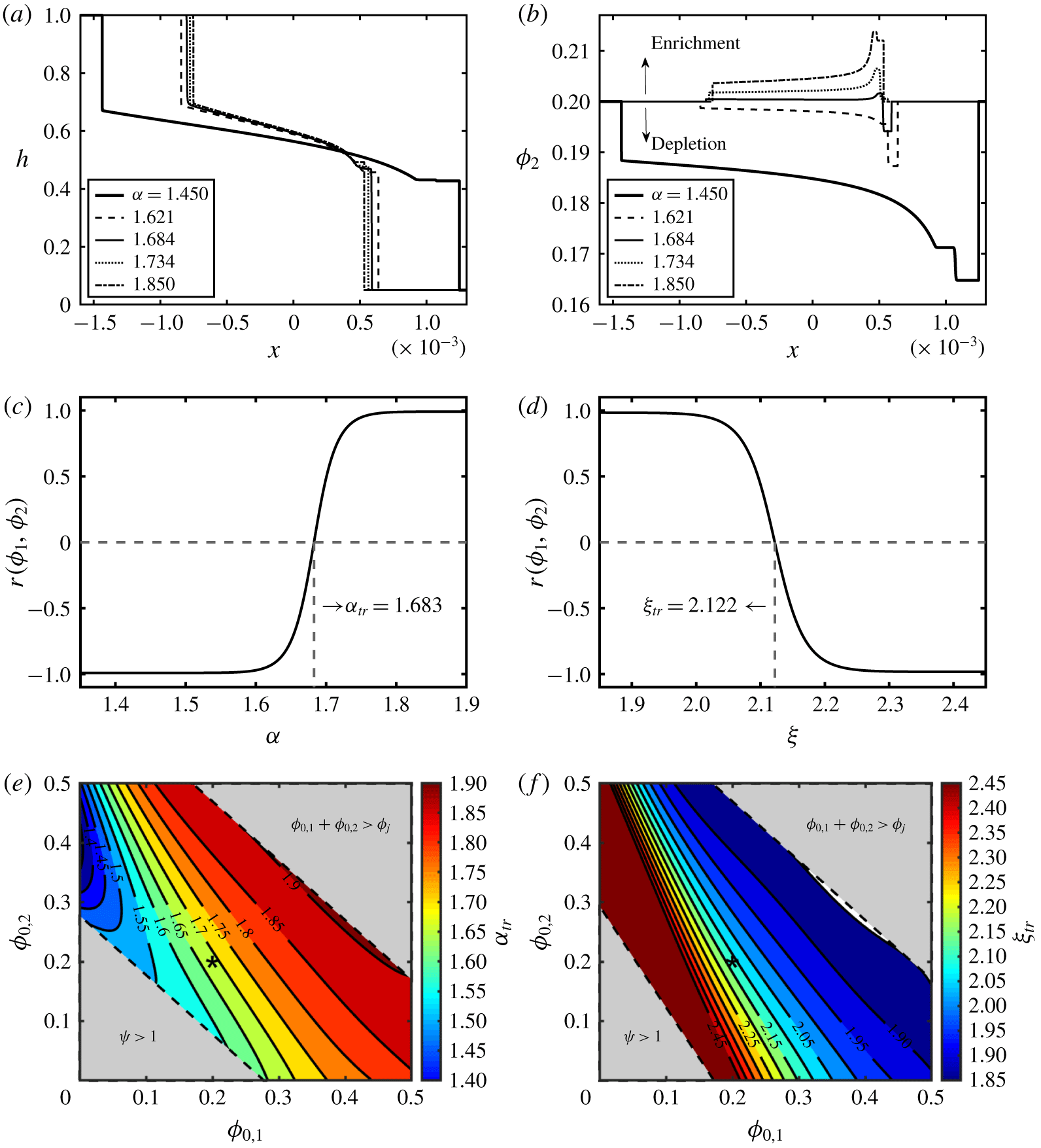
Change in (a) interface height,  $h$, and (b) particle volume fraction,
 $\unicode[STIX]{x1D719}_{2}$, with
 $x$ at
 $t=0.1$ and various values of particle type 2-to-carrying-fluid density ratio,
 $\unicode[STIX]{x1D6FC}$. Other parameters used are
 $\unicode[STIX]{x1D719}_{0,1}=\unicode[STIX]{x1D719}_{0,2}=0.2$,
 $Re=0.1$,
 $\unicode[STIX]{x1D705}=1$,
 $r_{p}=0.06$,
 $\unicode[STIX]{x1D709}=1.9$ and
 $\unicode[STIX]{x1D702}=1.25$. (c,d) Variation of the linear correlation coefficient,
 $r$, with
 $\unicode[STIX]{x1D6FC}$ for
 $\unicode[STIX]{x1D709}=1.9$ (c) and with
 $\unicode[STIX]{x1D709}$ for
 $\unicode[STIX]{x1D6FC}=1.85$ (d).
 $r$ can be represented by the Gudermannian function
 $Gd(z)=\arctan (\sinh (z))$, where
 $z$ is either
 $\unicode[STIX]{x1D6FC}$ or
 $\unicode[STIX]{x1D709}$. Note the transition from enrichment to depletion for particle type 2 in (c) occurs at
 $\unicode[STIX]{x1D6FC}_{tr}\approx 1.683$ and in (d) at
 $\unicode[STIX]{x1D709}_{tr}\approx 2.112$. (e,f) Phase diagrams of transition density ratio,
 $\unicode[STIX]{x1D6FC}_{tr}$ (e) and
 $\unicode[STIX]{x1D709}_{tr}$ (f), versus
 $\unicode[STIX]{x1D719}_{0,1}$ and
 $\unicode[STIX]{x1D719}_{0,2}$. The contour lines present different values of the properties
 $\unicode[STIX]{x1D6FC}_{tr}$ and
 $\unicode[STIX]{x1D709}_{tr}$. The top-right and bottom-left corners correspond to the jamming (
 $\unicode[STIX]{x1D719}_{0,1}+\unicode[STIX]{x1D719}_{0,2}>\unicode[STIX]{x1D719}_{j}$) and
 $\unicode[STIX]{x1D713}>1$ limits respectively (suspension lighter than pure fluid), which are beyond the scope of this study. Transition density ratios
 $\unicode[STIX]{x1D6FC}_{tr}$ and
 $\unicode[STIX]{x1D709}_{tr}$ are shown by
 $(\ast )$ markers in (e) and (f), respectively. The voided strip to the right of the lowest contour line in (f) is associated with
 $\unicode[STIX]{x1D709}_{tr}<1.85$ that is less than
 $\unicode[STIX]{x1D6FC}$, thus out of the parameter range.

In order to fully understand the enrichment–depletion transition mechanism, we need to choose refined values of  $\unicode[STIX]{x1D6FC}$ in the range [1.45–1.85]. Figures 5(a) and 5(b) depict the interface height,
 $h$, and particle type 2 volume fraction profiles,
 $\unicode[STIX]{x1D719}_{2}$, respectively for various values of
 $\unicode[STIX]{x1D6FC}$. The first thing to note from figure 5(a) is that the extent of the exchange zone between the heavy and light fluids diminishes with
 $\unicode[STIX]{x1D6FC}$. Figure 5(b) illustrates how
 $\unicode[STIX]{x1D719}_{2}$ transitions from enrichment behaviour to depletion when
 $\unicode[STIX]{x1D6FC}$ is decreased. It appears as though the transition density ratio,
 $\unicode[STIX]{x1D6FC}_{tr}\approx 1.684$, would result in approximately a neutral
 $\unicode[STIX]{x1D719}_{2}$ profile i.e. no bulk enrichment and/or depletion in the light particle volume fraction. Note that there can remain some interesting non-monotonic behaviours of the heavy front close to the transition threshold. For instance, the curve corresponding to
 $\unicode[STIX]{x1D6FC}=1.684$ in figure 5(b) shows enrichment in
 $\unicode[STIX]{x1D719}_{2}$, with some depletion occurring close to the very heavy frontal region. We did not observe a perfectly unvaried concentration profile of the light particles at
 $\unicode[STIX]{x1D6FC}_{tr}=1.684$ as was expected, nor at higher or lower values of
 $\unicode[STIX]{x1D6FC}$, meaning
 $\unicode[STIX]{x1D719}_{2}$ can still slightly oscillate around the initial concentration value,
 $\unicode[STIX]{x1D719}_{0,2}$, during the transition.
Given a constant particle type 1-to-carrying-fluid-density ratio,  $\unicode[STIX]{x1D709}$, the particle type 2-to-carrying-fluid-density ratio,
 $\unicode[STIX]{x1D6FC}$, practically becomes a measure of the density difference between the heavy and light particles (lower
 $\unicode[STIX]{x1D6FC}$ implying a much lighter particle type 2). We present that, for a given suspension, the density difference between two phases determines whether the particle type 2 phase is enriched or depleted along the interface. Although figure 5(b) provides a clear perspective on the enrichment–depletion mechanism, it does not produce further information to quantify
 $\unicode[STIX]{x1D6FC}_{tr}$ given other flow parameters. Based on the expressions for the slip velocities
 $u_{s,1}$ and
 $u_{s,2}$ ((2.20) and (2.21)) determining the mobility of particle types 1 and 2, one may assume that
 $\unicode[STIX]{x1D6FC}_{tr}$ would depend on the combined variation (i.e. covariance) of
 $\unicode[STIX]{x1D719}_{1}$ and
 $\unicode[STIX]{x1D719}_{2}$. Therefore, in order to systematically quantify the enrichment and depletion modes (thus obtaining
 $\unicode[STIX]{x1D6FC}_{tr}$), association between the
 $\unicode[STIX]{x1D719}_{1}$ and
 $\unicode[STIX]{x1D719}_{2}$ variables should be considered. We use the linear correlation coefficient, also called the product-moment correlation coefficient, or Pearson’s
 $r$ for this purpose; refer to Press (Reference Press1992). For a pair of quantities
 $\unicode[STIX]{x1D719}_{1}$ and
 $\unicode[STIX]{x1D719}_{2}$, the linear correlation coefficient,
 $r$, is given by the formula
 $$\begin{eqnarray}r(\unicode[STIX]{x1D719}_{1},\unicode[STIX]{x1D719}_{2})=\frac{S_{\unicode[STIX]{x1D719}_{1},\unicode[STIX]{x1D719}_{2}}}{S_{\unicode[STIX]{x1D719}_{1}}S_{\unicode[STIX]{x1D719}_{2}}},\end{eqnarray}$$
where  $S_{\unicode[STIX]{x1D719}_{1},\unicode[STIX]{x1D719}_{2}}$ is the covariance, and
 $S_{\unicode[STIX]{x1D719}_{1}}$ and
 $S_{\unicode[STIX]{x1D719}_{2}}$ are the standard deviations of the two volume fractions. The value of
 $r$ always lies between
 $-1$ to 1 and thus yields a tractable interpretation of covariance. Value of 1 is attributed to ‘complete positive correlation’ when
 $\unicode[STIX]{x1D719}_{1}$ and
 $\unicode[STIX]{x1D719}_{2}$ increasing together, which is closely associated with fully enriched flow in our simulations; see e.g. figure 4(b). On the other hand, ‘complete negative correlation’ is associated with the case when
 $\unicode[STIX]{x1D719}_{2}$ decreases as
 $\unicode[STIX]{x1D719}_{1}$ increases (
 $r=-1$ or depletion flows e.g. in figure 4d). Values of
 $r$ near zero indicate that
 $\unicode[STIX]{x1D719}_{1}$ and
 $\unicode[STIX]{x1D719}_{2}$ are uncorrelated. Since the heavy phase is always enriched, such values represent transitionary experiments in our study, where the light phase is neither enriched nor depleted. The variation of the correlation coefficient,
 $r(\unicode[STIX]{x1D719}_{1},\unicode[STIX]{x1D719}_{2})$, is demonstrated for different values of particle type 2-to-carrying-fluid density ratio,
 $\unicode[STIX]{x1D6FC}$, in figure 5(c) and for the values of particle type 1-to-carrying-fluid density ratio,
 $\unicode[STIX]{x1D709}$, in figure 5(d). From these figures, it is understood that the transition occurs rapidly as
 $r$ sharply changes sign from
 $-1$ to
 $+1$. It was observed that the data are best described by the Gudermannian function,
 $Gd(z)=\arctan (\sinh (z))$, where
 $z$ is either
 $\unicode[STIX]{x1D6FC}$ or
 $\unicode[STIX]{x1D709}$. The transition density ratio is obtained from this figure as
 $\unicode[STIX]{x1D6FC}_{tr}=1.683$, which is close to our initial estimate (
 $\unicode[STIX]{x1D6FC}_{tr}\approx 1.684$) from figure 5(b). In a similar fashion, the transition particle type 1-to-carrying-fluid density ratio is obtained as
 $\unicode[STIX]{x1D709}_{tr}=2.122$ according to figure 5(d).
We performed numerous distinct simulations (6490 tests) to obtain  $\unicode[STIX]{x1D6FC}_{tr}$ covering a range of
 $\unicode[STIX]{x1D719}_{0,1}$ and
 $\unicode[STIX]{x1D719}_{0,2}$ between 0 and 0.5. The results are shown in the phase diagram of figure 5(e). The transition density ratio,
 $\unicode[STIX]{x1D6FC}_{tr}$, appears to follow a fifth-order polynomial trend over the volume fraction domain. Note the contour lines simply represent a fitted surface on the calculated data points. The area near the bottom-left corner of the plot is associated with cases with
 $\unicode[STIX]{x1D713}>1$ (i.e. suspension lighter than pure fluid), therefore is out of the scope of this study. Also, the area at the top-right corner was left out as the total initial volume fraction of particles for such cases exceeds the jamming volume fraction, i.e.
 $\unicode[STIX]{x1D719}_{0,1}+\unicode[STIX]{x1D719}_{0,2}>\unicode[STIX]{x1D719}_{j}$. Strikingly, this figure shows that, by increasing the reference parameter,
 $\unicode[STIX]{x1D6FC}$, the flow changes from depletion to enrichment. In other words, if the density difference between particle types 1 and 2 remains constant, by adding more particles of any kind, having a depleted light phase in the flow is more likely to occur. Naturally, for fixed initial concentration values,
 $\unicode[STIX]{x1D719}_{0,1}$ and
 $\unicode[STIX]{x1D719}_{0,2}$, using particles with a smaller density difference (increasing
 $\unicode[STIX]{x1D6FC}$) can guarantee a circumstance where both heavy and light phase are enriched. Except for initial volume fractions nearing the jamming area, contours appear inclusively straight and parallel, with comparable inclination angles with respect to the axes. From figure 5(b), one can presume that, within the transitional flow, particle phase 2 is immobile with respect to its surrounding fluid. Curiously, setting the slip velocity of particle type 2,
 $u_{s,2}$, equal to zero in (2.21) would result in
 $\unicode[STIX]{x1D6FC}_{tr}=1-\unicode[STIX]{x1D719}_{0,1}(\unicode[STIX]{x1D709}-1)/[\unicode[STIX]{x1D719}_{0,2}+(\unicode[STIX]{x1D719}_{0,1}+\unicode[STIX]{x1D719}_{0,2})M_{o}/M_{I}]$ which slightly under-predicts the transition limit (
 $\unicode[STIX]{x1D6FC}_{tr}\approx 1.549$ versus 1.687 value obtained from figure 5e). This could be due to the fact that the interaction of the particle phases may not be fully captured under this condition, which requires further studies in the future.
We further produced a similar phase transition diagram for variable  $\unicode[STIX]{x1D709}_{tr}$, this time keeping
 $\unicode[STIX]{x1D6FC}$ fixed (figure 5f, 7716 tests). When the density difference between the two particle phases is small, i.e. low
 $\unicode[STIX]{x1D709}$, both particle populations tend to enrich along the interface. The implication is that by increasing
 $\unicode[STIX]{x1D709}$, the flow changes from enrichment to depletion (opposite trend to figure 5e). This diagram seems to complement the results of the
 $\unicode[STIX]{x1D6FC}_{tr}$ diagram. For instance, to avoid depletion of light particle events in the flow, when the initial concentrations of heavy and light particles are known, higher
 $\unicode[STIX]{x1D6FC}$ and lower
 $\unicode[STIX]{x1D709}$ are favourable conditions. Adding particles of any kind would shift the transition to occur at lower values of the density difference,
 $\unicode[STIX]{x1D709}$. This is opposite to figure 5(e), where the addition of particles causes the transition to happen at a higher density ratio,
 $\unicode[STIX]{x1D6FC}$. On the other hand, a similar examination with light-to-carrying-fluid density ratio,
 $\unicode[STIX]{x1D702}$, yields no discernible impact on the phase transition (results not presented for brevity). The reason can be found by considering the settling velocity relations (2.20) and (2.21), where
 $\unicode[STIX]{x1D702}$ is found in the denominator of both equations. Thus,
 $\unicode[STIX]{x1D702}$ expectedly controls both velocities to the same extent, dismissing a possible shift in phase transition. It is worth mentioning that the current authors observed an analogous effect in their experiments as well, where using fluids with different viscosities had no effect on mixing–settling transition of the particle-laden exchange flow; see Mirzaeian & Alba (Reference Mirzaeian and Alba2018b).
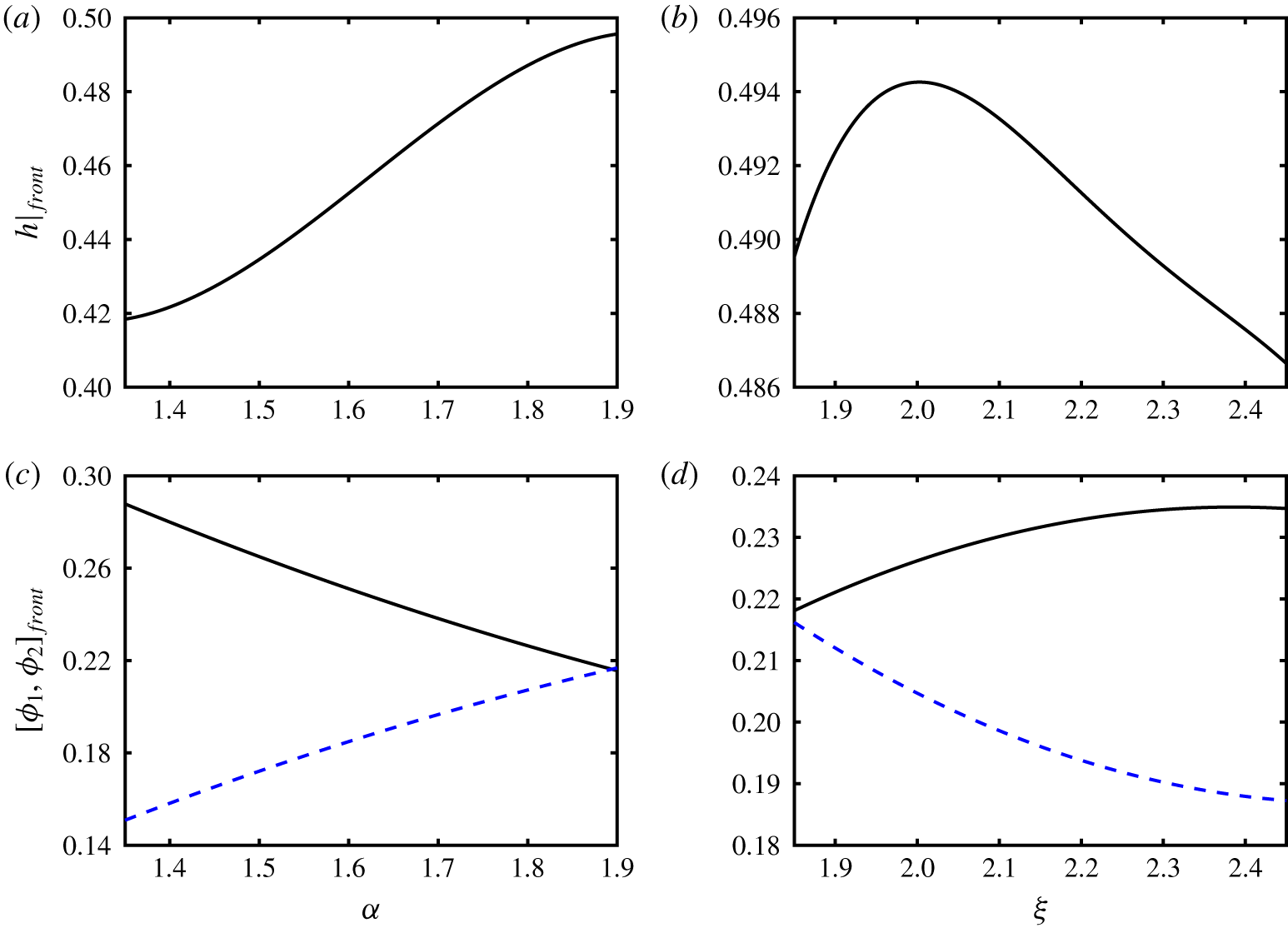
Change in interface height at the front,  $h|_{front}$, with (a) particle type 2-to-carrying-fluid density ratio
 $\unicode[STIX]{x1D6FC}$, and (b) particle type 1-to-carrying-fluid density ratio
 $\unicode[STIX]{x1D709}$ in fully developed flows. Other parameters used are
 $\unicode[STIX]{x1D719}_{0,1}=\unicode[STIX]{x1D719}_{0,2}=0.2$,
 $Re=0.1$,
 $\unicode[STIX]{x1D705}=1$,
 $r_{p}=0.06$ and
 $\unicode[STIX]{x1D702}=1.25$. Additionally, data were obtained by setting
 $\unicode[STIX]{x1D709}=1.9$ in (a), and
 $\unicode[STIX]{x1D6FC}=1.85$ in (b). The change in frontal properties
 $\unicode[STIX]{x1D719}_{1}|_{front}$ (line) and
 $\unicode[STIX]{x1D719}_{2}|_{front}$ (dashed line) with
 $\unicode[STIX]{x1D6FC}$ and
 $\unicode[STIX]{x1D709}$ are shown in (c) and (d), respectively.

Finally, we tracked the suspension front to determine the local values of the interface height,  $h|_{front}$, as well as concentrations of heavy and light particles,
 $\unicode[STIX]{x1D719}_{1}|_{front}$ and
 $\unicode[STIX]{x1D719}_{2}|_{front}$. We evaluated these parameters for values of
 $\unicode[STIX]{x1D6FC}\in [1.35,1.9]$ and
 $\unicode[STIX]{x1D709}\in [1.85,2.45]$, and plot the results in figure 6. We note that the particle type 1-to-carrying-fluid density ratio,
 $\unicode[STIX]{x1D709}=1.9$ is constant in figures 6(a) and 6(c), likewise, particle type 2-to-carrying-fluid density ratio,
 $\unicode[STIX]{x1D6FC}=1.85$ remains unchanged in figures 6(b) and 6(d). The following observations can be made. (i) The front height
 $h|_{front}$, increases monotonically with
 $\unicode[STIX]{x1D6FC}$ from 0.428 at
 $\unicode[STIX]{x1D6FC}=1.35$ to 0.496 at
 $\unicode[STIX]{x1D6FC}=1.9$ (figure 6a). The height initially increases with
 $\unicode[STIX]{x1D709}$ reaching a maximum value of
 $h|_{front}=0.494$, then it begins to decrease at around
 $\unicode[STIX]{x1D709}=2$ to an absolute minimum of 0.487 measured at
 $\unicode[STIX]{x1D709}=2.45$ (figure 6b). (ii) The volume fraction of heavy particles at the front,
 $\unicode[STIX]{x1D719}_{1}|_{front}$, drops from 0.288 at
 $\unicode[STIX]{x1D6FC}=1.35$ to 0.216 near
 $\unicode[STIX]{x1D6FC}=1.9$. Light particles are depleted at
 $\unicode[STIX]{x1D6FC}=1.35$ with their concentration
 $\unicode[STIX]{x1D719}_{2}|_{front}=0.151$ being less than their initial volume fraction,
 $\unicode[STIX]{x1D719}_{0,2}=0.2$, which gradually recovers to
 $\unicode[STIX]{x1D719}_{2}|_{front}\approx \unicode[STIX]{x1D719}_{1}|_{front}=0.216$ at
 $\unicode[STIX]{x1D6FC}=\unicode[STIX]{x1D709}=1.9$ (figure 6c). (iii) For
 $\unicode[STIX]{x1D6FC}=1.730$, the concentration of light particles at the front,
 $\unicode[STIX]{x1D719}_{2}|_{front}$, in figure 6(c) is equal to their initial concentration,
 $\unicode[STIX]{x1D719}_{0,2}=0.2$, that is higher than
 $\unicode[STIX]{x1D6FC}_{tr}=1.683$ predicted in figure 5(c). This is partly due to the interpolation error since
 $\unicode[STIX]{x1D719}_{2}|_{front}$ starts to oscillate at around the transition point, where
 $\unicode[STIX]{x1D719}_{1}$ and
 $\unicode[STIX]{x1D719}_{2}$ are uncorrelated, and it never actually become equal to 0.2. (iv) The total particle concentration in the front region,
 $\unicode[STIX]{x1D719}|_{front}=[\unicode[STIX]{x1D719}_{1}+\unicode[STIX]{x1D719}_{2}]_{front}$, minutely decreases from 0.439 to 0.432 as
 $\unicode[STIX]{x1D6FC}$ increases from 1.35 to 1.9; results are not shown in the figure for the sake of brevity. (v) By increasing
 $\unicode[STIX]{x1D709}$, volume fraction of the heavy particles,
 $\unicode[STIX]{x1D719}_{1}|_{front}$, slowly increases from 0.218 to the maximum value of 0.235 (figure 6d); meanwhile,
 $\unicode[STIX]{x1D719}_{2}|_{front}$ decreases from 0.217 (enriched) at
 $\unicode[STIX]{x1D709}=\unicode[STIX]{x1D6FC}=1.85$ to 0.187 (depleted) at
 $\unicode[STIX]{x1D709}=2.45$. (vi) The sum volume fraction of particles mildly decreases from
 $\unicode[STIX]{x1D719}|_{front}=0.439$ to 0.422 as
 $\unicode[STIX]{x1D709}$ changes from 1.85 to 2.45.
4.2 Parametric study
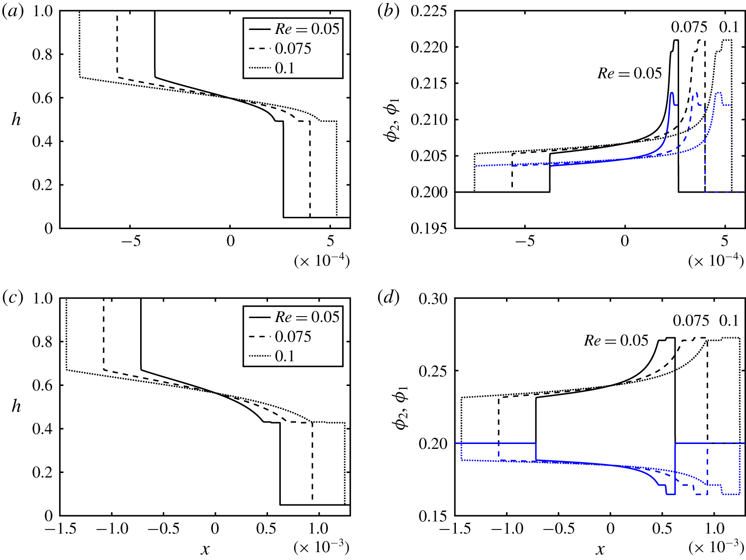
Change in (a) interface height,  $h$, and (b) particle volume fraction,
 $\unicode[STIX]{x1D719}$, with
 $x$ at
 $t=0.1$ and various values of the Reynolds number,
 $Re$. Other parameters used are
 $\unicode[STIX]{x1D719}_{0,1}=\unicode[STIX]{x1D719}_{0,2}=0.2$,
 $\unicode[STIX]{x1D705}=1$,
 $r_{p}=0.06$,
 $\unicode[STIX]{x1D709}=1.9$,
 $\unicode[STIX]{x1D6FC}=1.85$ and
 $\unicode[STIX]{x1D702}=1.25$. (c,d) The same as (a,b) obtained for
 $\unicode[STIX]{x1D6FC}=1.45$.

Mirzaeian & Alba (Reference Mirzaeian and Alba2018a) revealed that, in the case of monodensity suspensions, the height of the heavy layer front and its extent increase with precursor film thickness,  $b$. An increase in the frontal height is accompanied by a decrease in the level of particle enrichment. Similar effects are found in the bidensity limit for both enrichment and depletion cases. The results are not presented here for brevity. The picture given in figure 4 does not change much with
 $Re$ except an increase in
 $Re$ almost linearly increases the interpenetration rate of the heavy and light layers. The heavy and light frontal heights as well as the degree of particle enrichment remain approximately the same with
 $Re$, which is largely similar to the monodensity case of Mirzaeian & Alba (Reference Mirzaeian and Alba2018a). Keeping
 $\unicode[STIX]{x1D709}$ the same and changing
 $\unicode[STIX]{x1D6FC}$ as the transition parameter, figures 7(a,b) and 7(c,d) show the enrichment and depletion cases respectively.
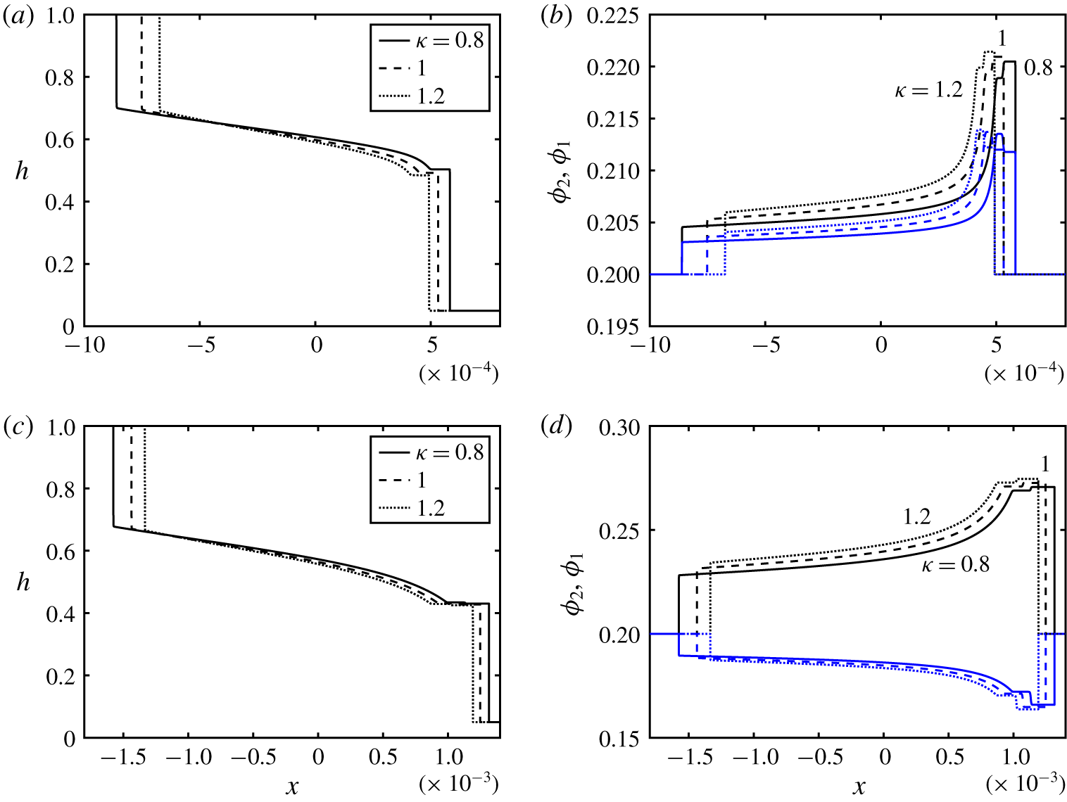
Change in (a) interface height,  $h$, and (b) particle volume fraction,
 $\unicode[STIX]{x1D719}$, with
 $x$ at
 $t=0.1$ and various values of the light-to-carrying-fluid viscosity ratio,
 $\unicode[STIX]{x1D705}$. Other parameters used are
 $\unicode[STIX]{x1D719}_{0,1}=\unicode[STIX]{x1D719}_{0,2}=0.2$,
 $Re=0.1$,
 $r_{p}=0.06$,
 $\unicode[STIX]{x1D709}=1.9$,
 $\unicode[STIX]{x1D6FC}=1.85$ and
 $\unicode[STIX]{x1D702}=1.25$. (c,d) The same as (a,b) obtained for
 $\unicode[STIX]{x1D6FC}=1.45$.

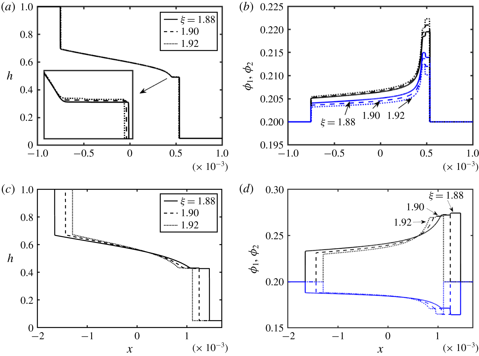
The effect of the light-to-carrying-fluid viscosity ratio,  $\unicode[STIX]{x1D705}$, on the exchange zone between the two fluids is shown in the enrichment (
 $\unicode[STIX]{x1D6FC}=1.85$ in figure 8a) and depletion cases (
 $\unicode[STIX]{x1D6FC}=1.45$ in figure 8c). The corresponding volume fraction profiles are given in figure 8(b,d). For more viscous heavy fluid (lower
 $\unicode[STIX]{x1D705}$), the degree of interpenetration of the layers is higher, which is in line with the findings of Taghavi et al. (Reference Taghavi, Seon, Martinez and Frigaard2009) and Matson & Hogg (Reference Matson and Hogg2012) for slumping flows. Keeping
 $Re=\hat{\unicode[STIX]{x1D70C}}_{H}(\unicode[STIX]{x1D719}_{0,1},\unicode[STIX]{x1D719}_{0,2})\hat{V}_{t}(2\hat{D})/\hat{\unicode[STIX]{x1D707}}_{H}(\unicode[STIX]{x1D719}_{0,1},\unicode[STIX]{x1D719}_{0,2})$ constant with more viscous heavy fluid (low
 $\unicode[STIX]{x1D705}$) requires larger
 $\hat{V}_{t}$ or a driving buoyancy force which then expands the extent of the exchange zone (figure 8a,c). Large
 $\unicode[STIX]{x1D705}$ corresponds to small
 $\hat{\unicode[STIX]{x1D707}}_{f,H}$, therefore, considering its definition, the dimensionless Stokes velocity,
 $u_{s}$ e.g. in (2.19), is increased as
 $\hat{\unicode[STIX]{x1D707}}_{f,H}$ is decreased. Larger
 $u_{s}$ increases the particle slip velocity in the
 $G$ and
 $Z$ flux functions (2.26) and (2.27) which will consequently result in a stronger accumulation of particles (or increased depletion of the light phase) as shown in figure 8(c,d).
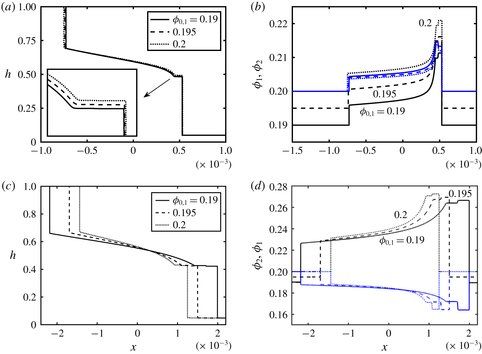
Change in (a) interface height,  $h$, and (b) particle volume fraction,
 $\unicode[STIX]{x1D719}$, with
 $x$ at
 $t=0.1$ and various values of the initial particle type 1 volume fraction,
 $\unicode[STIX]{x1D719}_{0,1}$. Other parameters used are
 $\unicode[STIX]{x1D719}_{0,2}=0.2$,
 $Re=0.1$,
 $\unicode[STIX]{x1D705}=1$,
 $r_{p}=0.06$,
 $\unicode[STIX]{x1D709}=1.9$,
 $\unicode[STIX]{x1D6FC}=1.85$ and
 $\unicode[STIX]{x1D702}=1.25$. (c,d) The same as (a,b) obtained for
 $\unicode[STIX]{x1D6FC}=1.45$.

The initial volume fractions of particles,  $\unicode[STIX]{x1D719}_{0,1}$ and
 $\unicode[STIX]{x1D719}_{0,2}$, play important roles in the dynamics of the flow since they control both the density and viscosity of the heavy suspension (2.3) and (2.4). The dependency of the interface height,
 $h$, and volume fraction of particles on
 $\unicode[STIX]{x1D719}_{0,1}$ is investigated in figures 9(a,b) and 9(c,d) respectively for the enrichment (
 $\unicode[STIX]{x1D6FC}=1.85$) and depletion cases (
 $\unicode[STIX]{x1D6FC}=1.45$). While the change in interface height profile,
 $h$, for the enrichment case is minimal (figure 9a), the extent of the interface is decreased with
 $\unicode[STIX]{x1D719}_{0,1}$, as shown in figure 9(c). As the density of the heavy suspension,
 $\hat{\unicode[STIX]{x1D70C}}_{H}$ increases with
 $\unicode[STIX]{x1D719}_{0,1}$ (larger driving force), its viscosity,
 $\hat{\unicode[STIX]{x1D707}}_{H}$, also increases, which results in an overall slowdown of the flow. Particle enrichment and depletion close to the heavy and light fronts are observed for various values of
 $\unicode[STIX]{x1D719}_{0,1}$ in figure 9(b,d). The discussion on suspensions in the dilute range of volume fraction (Segre & Silberberg Reference Segre and Silberberg1961) is provided in the monodensity model of Mirzaeian & Alba (Reference Mirzaeian and Alba2018a).
Change in (a) interface height,  $h$, and (b) particle volume fraction,
 $\unicode[STIX]{x1D719}$, with
 $x$ at
 $t=0.1$ and various values of the particles-radius-to-half-the-duct-width ratio,
 $r_{p}$. Other parameters used are
 $\unicode[STIX]{x1D719}_{0,1}=\unicode[STIX]{x1D719}_{0,2}=0.2$,
 $Re=0.1$,
 $\unicode[STIX]{x1D705}=1$,
 $\unicode[STIX]{x1D709}=1.9$,
 $\unicode[STIX]{x1D6FC}=1.85$ and
 $\unicode[STIX]{x1D702}=1.25$. (c,d) The same as (a,b) obtained for
 $\unicode[STIX]{x1D6FC}=1.45$.

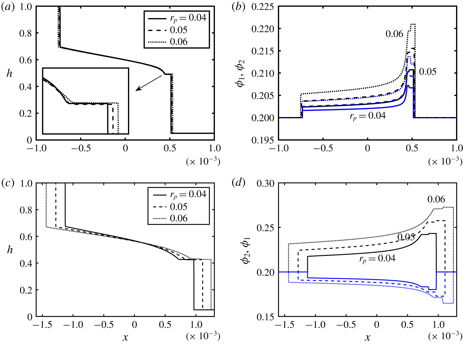
Investigating the effect of the size of the particles relative to the duct can provide more insight into the dynamics of the bidensity exchange flow in question. Figures 10(a,b) and 10(c,d) show the interface height and particle volume fraction profiles for the same parameters as the enrichment ( $\unicode[STIX]{x1D6FC}=1.85$) and depletion cases (
 $\unicode[STIX]{x1D6FC}=1.45$) in figure 4 except for different
 $r_{p}$. Note that particle types 1 and 2 are still assumed to have the same diameters. Increasing
 $r_{p}$ (larger particles) enhances the enrichment of both particle phases in figure 10(b), whereas increase in the size of the particles consistently enhances the level of enrichment in
 $\unicode[STIX]{x1D719}_{1}$ and depletion in
 $\unicode[STIX]{x1D719}_{2}$, as shown in figure 10(d). The interface between the two fluids has been extended with
 $r_{p}$, even though only slightly in the enrichment case (see inset of figure 10a). The increase in
 $r_{p}=\hat{a}/\hat{D}$ can be interpreted as either an increase in particle radius,
 $\hat{a}$, or a decrease in half of the duct width,
 $\hat{D}$. Since no theoretical bias exists for either case, we consider the latter. From the expression given in table 2, the Reynolds number,
 $Re$, should therefore decrease. Increasing
 $r_{p}$ while keeping
 $Re$ the same in figure 10 requires, for instance, a decrease in the heavy suspension viscosity,
 $\hat{\unicode[STIX]{x1D707}}_{H}(\unicode[STIX]{x1D719}_{0,1},\unicode[STIX]{x1D719}_{0,2})$, which is achievable by decreasing the carrying fluid viscosity,
 $\hat{\unicode[STIX]{x1D707}}_{f,H}$; see § 1.2. To maintain
 $\unicode[STIX]{x1D705}=\hat{\unicode[STIX]{x1D707}}_{L}/\hat{\unicode[STIX]{x1D707}}_{f,H}$ the same in figure 10,
 $\hat{\unicode[STIX]{x1D707}}_{L}$ should also be decreased. A decrease in the carrying and light fluids viscosities, on the other hand, eases the advancement of the exchange flow, as confirmed in figure 10(c). The effect of
 $r_{p}$ is, moreover, directly reflected in the particle dimensionless Stokes velocity (2.20) and (2.21), which feeds into the flux functions,
 $G$ and
 $Z$ in (2.26) and (2.27) respectively. An increase in
 $r_{p}$ enhances the settling speed of the particles, which in turn, causes pronounced accumulation of the heavy and light particles in the enrichment case (figure 10b) as well as intensified enrichment of the heavy particles and depletion of light particles close to the advancing frontal region in depletion flow (figure 10d).
Change in (a) interface height,  $h$, and (b) particle volume fraction,
 $\unicode[STIX]{x1D719}$, with
 $x$ at
 $t=0.1$ and various values of particle type 1 to carrying-fluid density ratio,
 $\unicode[STIX]{x1D709}$. Other parameters used are
 $\unicode[STIX]{x1D719}_{0,1}=\unicode[STIX]{x1D719}_{0,2}=0.2$,
 $Re=0.1$,
 $\unicode[STIX]{x1D705}=1$,
 $r_{p}=0.06$,
 $\unicode[STIX]{x1D702}=1.25$ and
 $\unicode[STIX]{x1D6FC}=1.85$. (c,d) The same as (a,b) obtained for
 $\unicode[STIX]{x1D6FC}=1.45$.

Another factor that can potentially affect the slip velocity of the particles is the particle type 1-to-carrying-fluid density ratio,  $\unicode[STIX]{x1D709}$; see figure 11. Note that the effect of the particle type 2-to-carrying-fluid density ratio,
 $\unicode[STIX]{x1D6FC}$, was studied earlier in figures 4 and 5. As opposed to
 $r_{p}$, an increase in
 $\unicode[STIX]{x1D709}$ reduces the interpenetration rate of the heavy and light layers; see the inset of figure 11(a) for enrichment as well as figure 11(c) for depletion cases respectively. Given that an increase in
 $\unicode[STIX]{x1D709}$ indicates heavier particles (increased buoyant driving force), at first glance, this effect appears to be rather counter-intuitive. However, similar to the rationale presented for figure 10, we need to consider the fact that the depicted profiles are plotted for a constant Reynolds number as a function of
 $\hat{V}_{t}$ which, by itself, decreases with
 $\unicode[STIX]{x1D713}$ since
 $\hat{V}_{t}=\sqrt{(1-\unicode[STIX]{x1D713}){\hat{g}}\hat{D}/(1+\unicode[STIX]{x1D713})}$. The parameter
 $\unicode[STIX]{x1D713}=\unicode[STIX]{x1D702}/(1+(\unicode[STIX]{x1D709}-1)\unicode[STIX]{x1D719}_{0,1}+(\unicode[STIX]{x1D6FC}-1)\unicode[STIX]{x1D719}_{0,2})$ is inversely related to
 $\unicode[STIX]{x1D709}$. Therefore, increasing
 $\unicode[STIX]{x1D709}$ (thus
 $\hat{V}_{t}$) while keeping
 $Re$ constant may be deduced as an increase in
 $\hat{\unicode[STIX]{x1D707}}_{H}(\unicode[STIX]{x1D719}_{0,1},\unicode[STIX]{x1D719}_{0,2})=\hat{\unicode[STIX]{x1D707}}_{f,H}(1-(\unicode[STIX]{x1D719}_{0,1}+\unicode[STIX]{x1D719}_{0,2})/\unicode[STIX]{x1D719}_{j})^{-2}$ or
 $\hat{\unicode[STIX]{x1D707}}_{f,H}$. Since the viscosity ratio,
 $\unicode[STIX]{x1D705}=\hat{\unicode[STIX]{x1D707}}_{L}/\hat{\unicode[STIX]{x1D707}}_{f,H}=1$, we shall then have increasing
 $\hat{\unicode[STIX]{x1D707}}_{L}$. As a result, flow deceleration will occur for higher values of
 $\unicode[STIX]{x1D709}$, which is correspondingly confirmed in figure 11(a,c). The effect of heavy (light) particle enrichment (depletion) appears to be different with
 $\unicode[STIX]{x1D709}$ for the
 $\unicode[STIX]{x1D6FC}=1.85$ and 1.45 cases shown in figures 11(b) and 11(d) respectively. As shown in figure 11(d), the increase in heavy particle enrichment for high
 $\unicode[STIX]{x1D709}$ (settling in a high viscosity medium) is slightly less than, but still comparable to, that of low
 $\unicode[STIX]{x1D709}$ owing to the higher density of solids in the former.
Change in (a) interface height,  $h$, and (b) particle volume fraction,
 $\unicode[STIX]{x1D719}$, with
 $x$ at
 $t=0.1$ and various values of the light-to-carrying-fluid density ratio,
 $\unicode[STIX]{x1D702}$. Other parameters used are
 $\unicode[STIX]{x1D719}_{0,1}=\unicode[STIX]{x1D719}_{0,2}=0.2$,
 $Re=0.1$,
 $\unicode[STIX]{x1D705}=1$,
 $r_{p}=0.06$,
 $\unicode[STIX]{x1D709}=1.9$ and
 $\unicode[STIX]{x1D6FC}=1.85$. (c,d) The same as (a,b) obtained for
 $\unicode[STIX]{x1D6FC}=1.45$.

The variation of the interface height,  $h$, and particle volume fraction,
 $\unicode[STIX]{x1D719}_{1}$ and
 $\unicode[STIX]{x1D719}_{2}$, with the light-to-carrying-fluid density ratio,
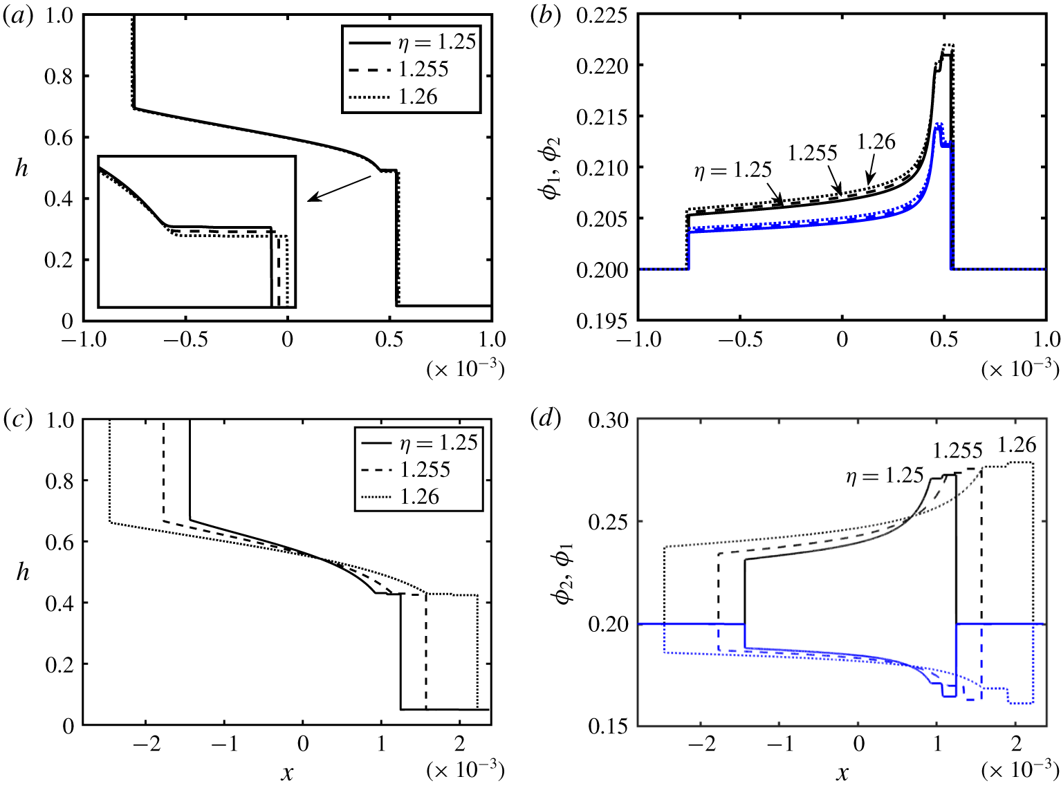
 $\unicode[STIX]{x1D702}$, is examined in figures 12(a,b) and 12(c,d) for enrichment and depletion cases respectively. The interpenetration extent of the fluids has increased with
 $\unicode[STIX]{x1D702}$; see inset of figure 12(a) as well as figure 12(c). Similar to figure 11, at first, this effect also appears counter-intuitive since an increase in
 $\unicode[STIX]{x1D702}$ may be interpreted as a denser light fluid compared to the carrying fluid i.e. a decrease in the effective density difference between the heavy and light fluids. However, increasing
 $\unicode[STIX]{x1D702}$ while keeping
 $Re$ the same in figure 12(c) requires e.g. a reduction in the viscosity of the involved fluids (
 $Re\propto \hat{\unicode[STIX]{x1D70C}}_{H}(\unicode[STIX]{x1D719}_{0,1},\unicode[STIX]{x1D719}_{0,2})/\hat{\unicode[STIX]{x1D707}}_{H}(\unicode[STIX]{x1D719}_{0,1},\unicode[STIX]{x1D719}_{0,2})$) which consequently enhances flow. As
 $\unicode[STIX]{x1D702}$ increases (while keeping
 $Re$ constant), fluids’ viscosities decrease, facilitating particles settling and thus enrichment in volume fraction,
 $\unicode[STIX]{x1D719}_{1}$, close to the fronts (figure 12b,d). The derivation of the model for an axisymmetric pipe geometry along with a brief discussion of results is given in appendix B.
5 Conclusions
Buoyancy-driven exchange flow of two fluids has been investigated theoretically in a vertical duct (2-D channel as well as pipe). The light fluid was assumed to be a pure fluid, and the heavy one a suspension containing two populations of negatively buoyant solid particles of the same size but different densities (bidensity). Assuming a small duct aspect ratio,  $\unicode[STIX]{x1D6FF}$, a lubrication model was developed following the methodology of Mirzaeian & Alba (Reference Mirzaeian and Alba2018a) carried out for monodensity flows. Shear-induced migration effects were neglected due to the particular Boussinesq approximation made (
 $At\ll \unicode[STIX]{x1D6FF}\ll 1$). The derived model took the form of the classical Riemann problem which was then solved numerically using a robust TVD finite difference scheme. Addition of a second type of particle vastly affected the solid phase slip velocity and thus the resulting governing equations. The dynamics of the flow was governed by eight dimensionless numbers namely the Reynolds number,
 $Re$, light-to-carrying-fluid viscosity ratio,
 $\unicode[STIX]{x1D705}$, initial volume fraction of heavy and light particles,
 $\unicode[STIX]{x1D719}_{0,1}$, and
 $\unicode[STIX]{x1D719}_{0,2}$, particle-diameter-to-duct-width ratio,
 $r_{p}$, heavy- and light-particle-to-carrying-fluid density ratios,
 $\unicode[STIX]{x1D709}$ and
 $\unicode[STIX]{x1D6FC}$, and the light-to-carrying-fluid density ratio,
 $\unicode[STIX]{x1D702}$. The only scenario previously observed in the monodensity case was particle enrichment in the vicinity of the advancing heavy and light fronts which occurred due to the different transport rates of the fluid and solid particles; see Mirzaeian & Alba (Reference Mirzaeian and Alba2018a). However, in the case of bidensity exchange flows an additional novel regime arose where there can be enrichment in the heavy particle phase but depletion in the light one. Keeping all the other parameters the same, the transition between the enrichment and depletion regimes was dictated by the ratios of the light and heavy particle densities to that of carrying fluid i.e.
 $\unicode[STIX]{x1D6FC}_{tr}$ and
 $\unicode[STIX]{x1D709}_{tr}$ respectively. The transition mechanism has been studied through additional simulations, revealing that
 $\unicode[STIX]{x1D6FC}_{tr}$ (
 $\unicode[STIX]{x1D709}_{tr}$) approximately increased (decreased) with increase in the initial volume fraction of particles. The
 $Re$ parameter enhanced the extent of the stretched the exchange zone between the heavy and light fluids with almost no effect on the level of particle enrichment and/or depletion. On the other hand, the parameter
 $\unicode[STIX]{x1D705}$ was shown to shrink the exchange zone and intensify particle enrichment and/or depletion. The effects of the rest of the parameters, namely
 $\unicode[STIX]{x1D719}_{0,1}$,
 $r_{p}$,
 $\unicode[STIX]{x1D709}$ and
 $\unicode[STIX]{x1D702}$, were furthermore discussed in this manuscript for both enrichment and depletion cases. The developed model paves the way to the study of more complicated scenarios such as polydisperse and/or non-Newtonian exchange flows in the future, which is of particular interest in many geophysical and industrial processes.
Acknowledgements
This research has been carried out at the University of Houston (UH) through National Research University Fund (NRUF) and the University of Texas at San Antonio. Useful discussion with Professor A. Bertozzi from the University of California Los Angeles (UCLA) is greatly appreciated. We thank the Center for Advanced Computing and Data Systems (CACDS) at UH and its helpful staff for providing us with their outstanding computational resources and assistance. Moreover, the reviewers are sincerely thanked for their helpful and constructive comments.
Declaration of interests
The authors report no conflict of interest.
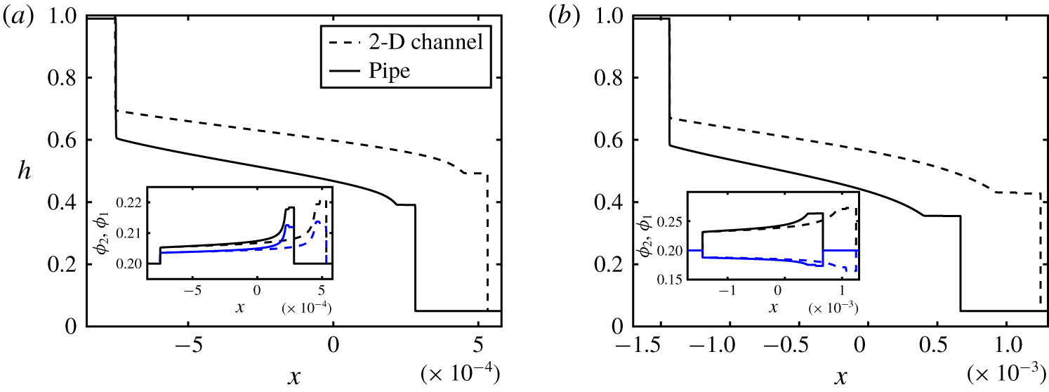
Appendix A. Shear-induced migration effects
Migration of particles induced by shear is in fact an important effect widely observed in particle-laden flows. Our methodology follows the approach of Zhou et al. (Reference Zhou, Dupuy, Bertozzi and Hosoi2005) for a gravity-driven suspension film down an incline which neglects the shear-induced migration effect; see also Schaflinger, Acrivos & Zhang (Reference Schaflinger, Acrivos and Zhang1990) and Acrivos, Fan & Mauri (Reference Acrivos, Fan and Mauri1994). In this appendix, we verify under which condition such an assumption is valid. The particle transport equation for particles  $i=1,2$ is given by Wong & Bertozzi (Reference Wong and Bertozzi2016) as
 $$\begin{eqnarray}\unicode[STIX]{x1D719}_{i,\hat{t}}+\hat{u} \unicode[STIX]{x1D719}_{i,\hat{x}}+\hat{v}\unicode[STIX]{x1D719}_{i,{\hat{y}}}=-\hat{\boldsymbol{J}}_{i\,\hat{x},\hat{x}}-\hat{\boldsymbol{J}}_{i{\hat{y}},{\hat{y}}},\quad i=1,2.\end{eqnarray}$$
Here,  $\hat{\boldsymbol{J}}_{i}$ is the particle
 $i$ flux due to settling, migration and mixing between particle types 1 and 2 caused by shear-induced migration
 $$\begin{eqnarray}\hat{\boldsymbol{J}}_{i}=\hat{\boldsymbol{J}}_{Settling,i}+\hat{\boldsymbol{J}}_{Migration,i}+\hat{\boldsymbol{J}}_{Tracer,i},\quad i=1,2.\end{eqnarray}$$
The flux components in (A 2) can be expressed as the following, see Murisic et al. (Reference Murisic, Pausader, Peschka and Bertozzi2013) and Wong & Bertozzi (Reference Wong and Bertozzi2016),
 $$\begin{eqnarray}\displaystyle \hat{\boldsymbol{J}}_{Settling,i}=\frac{2\hat{a}^{2}{\hat{g}}}{9\hat{\unicode[STIX]{x1D707}}_{f,H}}\left[M_{o}(\hat{\unicode[STIX]{x1D70C}}_{p,i}-\hat{\unicode[STIX]{x1D70C}}_{f,H})+M_{I}\mathop{\sum }_{k=1}^{2}(\hat{\unicode[STIX]{x1D70C}}_{p,k}-\hat{\unicode[STIX]{x1D70C}}_{f,H})\frac{\unicode[STIX]{x1D719}_{k}}{\unicode[STIX]{x1D719}_{1}+\unicode[STIX]{x1D719}_{2}}\right]\unicode[STIX]{x1D719}_{i},\quad i=1,2,\end{eqnarray}$$
 $$\begin{eqnarray}\displaystyle \displaystyle \hat{\boldsymbol{J}}_{Migration,i} & = & \displaystyle -\frac{\hat{a}^{2}\hat{V}_{t}}{\hat{D}^{2}}\left[K_{c}(\unicode[STIX]{x1D719}_{1}+\unicode[STIX]{x1D719}_{2})\unicode[STIX]{x1D735}((\unicode[STIX]{x1D719}_{1}+\unicode[STIX]{x1D719}_{2})u_{y})+\frac{K_{v}(\unicode[STIX]{x1D719}_{1}+\unicode[STIX]{x1D719}_{2})^{2}u_{y}}{\unicode[STIX]{x1D707}_{H}}\unicode[STIX]{x1D735}\unicode[STIX]{x1D707}_{H}\right]\nonumber\\ \displaystyle & & \displaystyle \times \,\frac{\unicode[STIX]{x1D719}_{i}}{\unicode[STIX]{x1D719}_{1}+\unicode[STIX]{x1D719}_{2}},\quad i=1,2,\end{eqnarray}$$
 $$\begin{eqnarray}\displaystyle \hat{\boldsymbol{J}}_{Tracer,i}=\frac{\hat{a}^{2}\hat{V}_{t}}{2\hat{D}^{2}}(\unicode[STIX]{x1D719}_{1}+\unicode[STIX]{x1D719}_{2})u_{y}D_{tr}\unicode[STIX]{x1D735}\left(\frac{\unicode[STIX]{x1D719}_{i}}{\unicode[STIX]{x1D719}_{1}+\unicode[STIX]{x1D719}_{2}}\right),\quad i=1,2.\end{eqnarray}$$
The constants  $K_{c}\approx 0.41$ and
 $K_{v}\approx 0.62$ correspond to the shear-induced particle flux due to the gradients in the particle volume fraction and effective viscosity of the suspension, which are determined empirically; see Phillips et al. (Reference Phillips, Armstrong, Brown, Graham and Abbott1992) and Wong & Bertozzi (Reference Wong and Bertozzi2016). Moreover,
 $D_{tr}$ is the modified tracer diffusivity chosen as
 $D_{tr}=\min \{(\unicode[STIX]{x1D719}_{1}+\unicode[STIX]{x1D719}_{2})^{2},0.4^{2}\}$; see Leighton & Acrivos (Reference Leighton and Acrivos1986, Reference Leighton and Acrivos1987), Sierou & Brady (Reference Sierou and Brady2004) and Lee et al. (Reference Lee, Wong and Bertozzi2015). From the velocity expression (2.11), it can be found that
 $u_{y}\sim Re$; see also appendix C for the coefficients of
 $u$. In order to have the settling effect dominate that of migration, the
 $\hat{x}$-derivative of the smallest dimensional flux coefficient in (A 3) i.e.
 $2\hat{a}^{2}{\hat{g}}(\hat{\unicode[STIX]{x1D70C}}_{p,i}-\hat{\unicode[STIX]{x1D70C}}_{f,H})/(9\hat{\unicode[STIX]{x1D707}}_{f,H})$, should be much larger than the
 ${\hat{y}}$-derivative of the largest flux components in (A 4) and (A 5) i.e.
 $\hat{a}^{2}K_{v}\hat{V}_{t}Re/\hat{D}^{2}$ and
 $\hat{a}^{2}\hat{V}_{t}Re/(2\hat{D}^{2})$ respectively. Note that the rest of the terms in (A 3) and (A 4) multiplied by these coefficients are
 $O(1)$ since they are made dimensionless. As such, the following condition is finally obtained
 $$\begin{eqnarray}\frac{9K_{v}\unicode[STIX]{x1D702}(1-(\unicode[STIX]{x1D719}_{0,1}+\unicode[STIX]{x1D719}_{0,2})/\unicode[STIX]{x1D719}_{j})^{2}}{\min \{(\unicode[STIX]{x1D709}-1),(\unicode[STIX]{x1D6FC}-1)\}\unicode[STIX]{x1D713}}\frac{(1-\unicode[STIX]{x1D713})}{(1+\unicode[STIX]{x1D713})}\ll \unicode[STIX]{x1D6FF}\ll 1.\end{eqnarray}$$
The  $(1-\unicode[STIX]{x1D713})/(1+\unicode[STIX]{x1D713})$ term in (A 6) is merely the effective Atwood number,
 $At=(\hat{\unicode[STIX]{x1D70C}}_{H}(\unicode[STIX]{x1D719}_{0,1},\unicode[STIX]{x1D719}_{0,2})-\hat{\unicode[STIX]{x1D70C}}_{L})/(\hat{\unicode[STIX]{x1D70C}}_{H}(\unicode[STIX]{x1D719}_{0,1},\unicode[STIX]{x1D719}_{0,2})+\hat{\unicode[STIX]{x1D70C}}_{L})$. In other words, the particular Boussinesq limit (
 $At\ll \unicode[STIX]{x1D6FF}\ll 1$) ensures that the shear-induced migration effects are negligible as compared to settling. Note that the rest of the terms in (A 6) are approximately
 $O(1)$. In a broader context, the aspect ratio parameter,
 $\unicode[STIX]{x1D6FF}=\hat{D}/\hat{L}$, may be considered as a function of time,
 $\hat{t}$, meaning that, as time goes by, the extent of the exchange zone between the heavy and light fluids,
 $\hat{L}(\,\hat{t}\,)$, increases. In such a case, over time, the lubrication approximation (uniform volume fraction assumption) can become more (less) accurate with the opposite effect observed at short times. There can perhaps exist a time range where both assumptions are correct, which requires further experimental and/or DNS studies. Here, for simplicity and the sake of consistency with the scaling adopted in § 1.1, we assume that the duct length,
 $\hat{L}$, is fixed, which results in a small constant
 $\unicode[STIX]{x1D6FF}\ll 1$. Therefore, as long as the Atwood number,
 $At$, is chosen to be smaller than
 $\unicode[STIX]{x1D6FF}$, the lubrication model remains consistent. It is confirmed that, for a typical set of parameters chosen in our study, the left-hand side term in condition (A 6) is indeed a small number (e.g.
 ${\approx}0.055$ in figure 4). Note that readers are advised to consider this revised notion,
 $At\ll \unicode[STIX]{x1D6FF}\ll 1$, instead of
 $At\ll 1$ previously derived by Mirzaeian & Alba (Reference Mirzaeian and Alba2018a).
Appendix B. Axisymmetric flow in pipe
Schematic of the symmetric bidensity particle-laden exchange flow in a vertical 3-D pipe ( $\hat{\unicode[STIX]{x1D70C}}_{p,1}>\hat{\unicode[STIX]{x1D70C}}_{p,2}$).

The schematic configuration of bidensity exchange flow is depicted in figure 13. In cylindrical coordinates, the momentum equations (2.9) and (2.10) take the following form
 $$\begin{eqnarray}\displaystyle & 0=-P_{0,x}+\unicode[STIX]{x1D707}_{H}(\unicode[STIX]{x1D719}_{1},\unicode[STIX]{x1D719}_{2})(ru_{r})_{r}/r,\quad 1-h\leqslant r\leqslant 1, & \displaystyle\end{eqnarray}$$
 $$\begin{eqnarray}\displaystyle & 0=-P_{0,x}-(\unicode[STIX]{x1D70C}_{H}(\unicode[STIX]{x1D719}_{1},\unicode[STIX]{x1D719}_{2})-\unicode[STIX]{x1D713})Re/(1-\unicode[STIX]{x1D713})+m(ru_{r})_{r}/r,\quad 0\leqslant y\leqslant 1-h. & \displaystyle\end{eqnarray}$$
Applying appropriate boundary and interfacial conditions, (B 1) and (B 2) can be integrated with respect to  $r$ in order to determine the streamwise velocity closures in each layer. The flux function,
 $q=\hat{q}/(\unicode[STIX]{x03C0}\hat{D}^{2}\hat{V}_{t})$, and the flow rate within the heavy layer can then be calculated as
 $$\begin{eqnarray}q=2\int _{1-h}^{1}ru\,\text{d}r,\end{eqnarray}$$
which is given below in terms of  $h$,
 $Re$,
 $m$,
 $\unicode[STIX]{x1D707}_{H}$ and
 $\unicode[STIX]{x1D70C}_{H}$.
 $$\begin{eqnarray}\displaystyle q & = & \displaystyle -(1/8)Re(-4\ln (1-h)\unicode[STIX]{x1D707}_{H}\unicode[STIX]{x1D713}-104h^{6}m\unicode[STIX]{x1D713}-144h^{5}\unicode[STIX]{x1D707}_{H}\unicode[STIX]{x1D713}+176h^{5}m\unicode[STIX]{x1D713}-80h^{3}m\unicode[STIX]{x1D70C}_{H}\nonumber\\ \displaystyle & & \displaystyle +\,16h^{2}m\unicode[STIX]{x1D70C}_{H}+164h^{4}m\unicode[STIX]{x1D70C}_{H}+144h^{5}\unicode[STIX]{x1D707}_{H}\unicode[STIX]{x1D70C}_{H}+104h^{6}m\unicode[STIX]{x1D70C}_{H}+80h^{6}\unicode[STIX]{x1D707}_{H}\unicode[STIX]{x1D713}+92h^{3}\unicode[STIX]{x1D707}_{H}\unicode[STIX]{x1D70C}_{H}\nonumber\\ \displaystyle & & \displaystyle -\,30h^{2}\unicode[STIX]{x1D707}_{H}\unicode[STIX]{x1D70C}_{H}+4h\unicode[STIX]{x1D707}_{H}\unicode[STIX]{x1D70C}_{H}-4h^{8}m\unicode[STIX]{x1D713}+32h^{7}m\unicode[STIX]{x1D713}+4h^{8}m\unicode[STIX]{x1D70C}_{H}-32h^{7}m\unicode[STIX]{x1D70C}_{H}-24h^{7}\unicode[STIX]{x1D707}_{H}\unicode[STIX]{x1D713}\nonumber\\ \displaystyle & & \displaystyle +\,24h^{7}\unicode[STIX]{x1D707}_{H}\unicode[STIX]{x1D70C}_{H}+3h^{8}\unicode[STIX]{x1D707}_{H}\unicode[STIX]{x1D713}-3h^{8}\unicode[STIX]{x1D707}_{H}\unicode[STIX]{x1D70C}_{H}+280\ln (1-h)h^{4}\unicode[STIX]{x1D707}_{H}\unicode[STIX]{x1D70C}_{H}-208\ln (1-h)h^{3}m\unicode[STIX]{x1D713}\nonumber\\ \displaystyle & & \displaystyle +\,208\ln (1-h)h^{3}m\unicode[STIX]{x1D70C}_{H}+224\ln (1-h)h^{3}\unicode[STIX]{x1D707}_{H}\unicode[STIX]{x1D713}-224\ln (1-h)h^{3}\unicode[STIX]{x1D707}_{H}\unicode[STIX]{x1D70C}_{H}\nonumber\\ \displaystyle & & \displaystyle -\,112\ln (1-h)h^{2}\unicode[STIX]{x1D707}_{H}\unicode[STIX]{x1D713}+112\ln (1-h)h^{2}\unicode[STIX]{x1D707}_{H}\unicode[STIX]{x1D70C}_{H}+32\ln (1-h)h\unicode[STIX]{x1D707}_{H}\unicode[STIX]{x1D713}\nonumber\\ \displaystyle & & \displaystyle -\,32\ln (1-h)h\unicode[STIX]{x1D707}_{H}\unicode[STIX]{x1D70C}_{H}+88\ln (1-h)h^{2}m\unicode[STIX]{x1D713}-88\ln (1-h)h^{2}m\unicode[STIX]{x1D70C}_{H}\nonumber\\ \displaystyle & & \displaystyle -\,16\ln (1-h)hm\unicode[STIX]{x1D713}+16\ln (1-h)hm\unicode[STIX]{x1D70C}_{H}+4\ln (1-h)h^{8}m\unicode[STIX]{x1D713}-32\ln (1-h)h^{7}m\unicode[STIX]{x1D713}\nonumber\\ \displaystyle & & \displaystyle -\,4\ln (1-h)h^{8}m\unicode[STIX]{x1D70C}_{H}+32\ln (1-h)h^{7}m\unicode[STIX]{x1D70C}_{H}-4\ln (1-h)h^{8}\unicode[STIX]{x1D707}_{H}\unicode[STIX]{x1D713}\nonumber\\ \displaystyle & & \displaystyle +\,32\ln (1-h)h^{7}\unicode[STIX]{x1D707}_{H}\unicode[STIX]{x1D713}+4\ln (1-h)h^{8}\unicode[STIX]{x1D707}_{H}\unicode[STIX]{x1D70C}_{H}-32\ln (1-h)h^{7}\unicode[STIX]{x1D707}_{H}\unicode[STIX]{x1D70C}_{H}\nonumber\\ \displaystyle & & \displaystyle +\,112\ln (1-h)h^{6}m\unicode[STIX]{x1D713}-112\ln (1-h)h^{6}m\unicode[STIX]{x1D70C}_{H}-112\ln (1-h)h^{6}\unicode[STIX]{x1D707}_{H}\unicode[STIX]{x1D713}\nonumber\\ \displaystyle & & \displaystyle +\,112\ln (1-h)h^{6}\unicode[STIX]{x1D707}_{H}\unicode[STIX]{x1D70C}_{H}-224\ln (1-h)h^{5}m\unicode[STIX]{x1D713}+224\ln (1-h)h^{5}m\unicode[STIX]{x1D70C}_{H}\nonumber\\ \displaystyle & & \displaystyle +\,224\ln (1-h)h^{5}\unicode[STIX]{x1D707}_{H}\unicode[STIX]{x1D713}-224\ln (1-h)h^{5}\unicode[STIX]{x1D707}_{H}\unicode[STIX]{x1D70C}_{H}+276\ln (1-h)h^{4}m\unicode[STIX]{x1D713}\nonumber\\ \displaystyle & & \displaystyle -\,276\ln (1-h)h^{4}m\unicode[STIX]{x1D70C}_{H}-280\ln (1-h)h^{4}\unicode[STIX]{x1D707}_{H}\unicode[STIX]{x1D713}-92h^{3}\unicode[STIX]{x1D707}_{H}\unicode[STIX]{x1D713}-164h^{4}m\unicode[STIX]{x1D713}\nonumber\\ \displaystyle & & \displaystyle -\,4h\unicode[STIX]{x1D707}_{H}\unicode[STIX]{x1D713}+30h^{2}\unicode[STIX]{x1D707}_{H}\unicode[STIX]{x1D713}+80h^{3}m\unicode[STIX]{x1D713}-16h^{2}m\unicode[STIX]{x1D713}+151h^{4}\unicode[STIX]{x1D707}_{H}\unicode[STIX]{x1D713}-151h^{4}\unicode[STIX]{x1D707}_{H}\unicode[STIX]{x1D70C}_{H}\nonumber\\ \displaystyle & & \displaystyle -\,80h^{6}\unicode[STIX]{x1D707}_{H}\unicode[STIX]{x1D70C}_{H}-176h^{5}m\unicode[STIX]{x1D70C}_{H}+4\ln (1-h)\unicode[STIX]{x1D707}_{H}\unicode[STIX]{x1D70C}_{H})/(\unicode[STIX]{x1D707}_{H} (h^{4}m\unicode[STIX]{x1D713}-h^{4}\unicode[STIX]{x1D707}_{H}\unicode[STIX]{x1D713}-h^{4}m\nonumber\\ \displaystyle & & \displaystyle +\,h^{4}\unicode[STIX]{x1D707}_{H}-4h^{3}m\unicode[STIX]{x1D713}+4h^{3}\unicode[STIX]{x1D707}_{H}\unicode[STIX]{x1D713}+4h^{3}m-4h^{3}\unicode[STIX]{x1D707}_{H}+6h^{2}m\unicode[STIX]{x1D713}-6h^{2}\unicode[STIX]{x1D707}_{H}\unicode[STIX]{x1D713}-6h^{2}m\nonumber\\ \displaystyle & & \displaystyle +\,6h^{2}\unicode[STIX]{x1D707}_{H}-4hm\unicode[STIX]{x1D713}+4h\unicode[STIX]{x1D707}_{H}\unicode[STIX]{x1D713}+4hm-4h\unicode[STIX]{x1D707}_{H}-\unicode[STIX]{x1D707}_{H}\unicode[STIX]{x1D713}+\unicode[STIX]{x1D707}_{H})).\end{eqnarray}$$
The evolution equations for the interface height and particle volume fraction respectively are
 $$\begin{eqnarray}\displaystyle & H_{t}+F_{x}(H,\unicode[STIX]{x1D6E9}_{1},\unicode[STIX]{x1D6E9}_{2})=0, & \displaystyle\end{eqnarray}$$
 $$\begin{eqnarray}\displaystyle & \unicode[STIX]{x1D6E9}_{1,t}+G_{x}(H,\unicode[STIX]{x1D6E9}_{1},\unicode[STIX]{x1D6E9}_{2})=0, & \displaystyle\end{eqnarray}$$
 $$\begin{eqnarray}\displaystyle & \unicode[STIX]{x1D6E9}_{2,t}+Z_{x}(H,\unicode[STIX]{x1D6E9}_{1},\unicode[STIX]{x1D6E9}_{2})=0, & \displaystyle\end{eqnarray}$$
where,  $H=(1-h)^{2}$,
 $\unicode[STIX]{x1D6E9}_{1}=\unicode[STIX]{x1D703}_{1}(1-(1-h)^{2})/h$,
 $\unicode[STIX]{x1D6E9}_{2}=\unicode[STIX]{x1D703}_{2}(1-(1-h)^{2})/h$ and
 $$\begin{eqnarray}F(H,\unicode[STIX]{x1D6E9}_{1},\unicode[STIX]{x1D6E9}_{2})=-q(H,\unicode[STIX]{x1D6E9}_{1},\unicode[STIX]{x1D6E9}_{2}),\end{eqnarray}$$
 $$\begin{eqnarray}\displaystyle \displaystyle G(H,\unicode[STIX]{x1D6E9}_{1},\unicode[STIX]{x1D6E9}_{2}) & = & \displaystyle -\frac{\unicode[STIX]{x1D6E9}_{1}F(H,\unicode[STIX]{x1D6E9}_{1},\unicode[STIX]{x1D6E9}_{2})}{1-H}+\unicode[STIX]{x1D6E9}_{1}\left(1-\frac{\unicode[STIX]{x1D6E9}_{1}}{1-H}\right)u_{s,1}(H,\unicode[STIX]{x1D6E9}_{1},\unicode[STIX]{x1D6E9}_{2})\nonumber\\ \displaystyle & & \displaystyle -\,\unicode[STIX]{x1D6E9}_{1}\unicode[STIX]{x1D6E9}_{2}u_{s,2}(H,\unicode[STIX]{x1D6E9}_{1},\unicode[STIX]{x1D6E9}_{2}),\end{eqnarray}$$
 $$\begin{eqnarray}\displaystyle Z(H,\unicode[STIX]{x1D6E9}_{1},\unicode[STIX]{x1D6E9}_{2}) & = & \displaystyle -\frac{\unicode[STIX]{x1D6E9}_{2}F(H,\unicode[STIX]{x1D6E9}_{1},\unicode[STIX]{x1D6E9}_{2})}{1-H}-\unicode[STIX]{x1D6E9}_{2}\unicode[STIX]{x1D6E9}_{1}u_{s,1}(H,\unicode[STIX]{x1D6E9}_{1},\unicode[STIX]{x1D6E9}_{2})\nonumber\\ \displaystyle & & \displaystyle +\,\unicode[STIX]{x1D6E9}_{2}\left(1-\frac{\unicode[STIX]{x1D6E9}_{2}}{1-H}\right)u_{s,2}(H,\unicode[STIX]{x1D6E9}_{1},\unicode[STIX]{x1D6E9}_{2}).\end{eqnarray}$$
Using the exact same numerical scheme as the one explained in the text, PDEs (B 5)–(B 7) can be solved to give evolution of  $H$ and
 $\unicode[STIX]{x1D6E9}$ (thus
 $h$ and
 $\unicode[STIX]{x1D719}$) in space,
 $x$, and time,
 $t$. Figures 14(a) and 14(b) compare the pipe interface profile against that of the 2-D channel shown earlier in figure 4 for enrichment and depletion cases respectively. The inset depicts the corresponding profiles of particle volume fractions,
 $\unicode[STIX]{x1D719}_{1}$ and
 $\unicode[STIX]{x1D719}_{2}$. Similar particle enrichment effect as in the 2-D channel case is observed with slight modification due to the geometric difference. Figure 14 depicts that the heavy and light frontal height,
 $h$, is larger in the case of channel compared to the pipe with the exchange flow appearing to advance more rapidly in the former. Furthermore, similar to the monodensity case of Mirzaeian & Alba (Reference Mirzaeian and Alba2018a), the level of particle enrichment is slightly lower in the pipe than the channel; see inset in figure 14(a). The vertical pipe experiments presented in our previous work by Mirzaeian & Alba (Reference Mirzaeian and Alba2018b) exhibit some level of asymmetry, therefore making a direct comparison with current theoretical work infeasible. A major factor that promotes the side-by-side pattern in experiments is the design and operation of the gate valve (double-acting pneumatic-solenoid actuator from VAT Group AG valves). Additional experiments need to be carefully designed to compare against our current model. As well as matching the fluid and particle densities, a special gate valve needs to be considered to closely mimic the flow configuration assumed in the lubrication model, which is suspension wetting the wall and pure fluid moving through the core.


Appendix C. Coefficients of velocity expressions (2.11) and (2.12) for 2-D channel case
 $$\begin{eqnarray}\displaystyle P_{0,x} & = & \displaystyle -[(3h^{3}m-2h^{3}\unicode[STIX]{x1D707}_{H}-9h^{2}m+6h^{2}\unicode[STIX]{x1D707}_{H}+6hm-6h\unicode[STIX]{x1D707}_{H}+2\unicode[STIX]{x1D707}_{H})\unicode[STIX]{x1D713}-3h^{3}m\unicode[STIX]{x1D70C}_{H}\nonumber\\ \displaystyle & & \displaystyle +\,2h^{3}\unicode[STIX]{x1D707}_{H}\unicode[STIX]{x1D70C}_{H}+9h^{2}m\unicode[STIX]{x1D70C}_{H}-6h^{2}\unicode[STIX]{x1D707}_{H}\unicode[STIX]{x1D70C}_{H}-6hm\unicode[STIX]{x1D70C}_{H}+6h\unicode[STIX]{x1D707}_{H}\unicode[STIX]{x1D70C}_{H}-2\unicode[STIX]{x1D707}_{H}\unicode[STIX]{x1D70C}_{H}]Re/\nonumber\\ \displaystyle & & \displaystyle [2(\unicode[STIX]{x1D713}-1)(h^{3}m-h^{3}\unicode[STIX]{x1D707}_{H}-3h^{2}m+3h^{2}\unicode[STIX]{x1D707}_{H}+3hm-3h\unicode[STIX]{x1D707}_{H}+\unicode[STIX]{x1D707}_{H})],\end{eqnarray}$$
 $$\begin{eqnarray}\displaystyle c_{1} & = & \displaystyle [(2h^{3}m-2h^{3}\unicode[STIX]{x1D707}_{H}-5h^{2}m+6h^{2}\unicode[STIX]{x1D707}_{H}+3hm-6h\unicode[STIX]{x1D707}_{H}+2\unicode[STIX]{x1D707}_{H})\unicode[STIX]{x1D713}-2h^{3}m\unicode[STIX]{x1D70C}_{H}\nonumber\\ \displaystyle & & \displaystyle +\,2h^{3}\unicode[STIX]{x1D707}_{H}\unicode[STIX]{x1D70C}_{H}+5h^{2}m\unicode[STIX]{x1D70C}_{H}-6h^{2}\unicode[STIX]{x1D707}_{H}\unicode[STIX]{x1D70C}_{H}-3hm\unicode[STIX]{x1D70C}_{H}+6h\unicode[STIX]{x1D707}_{H}\unicode[STIX]{x1D70C}_{H}-2\unicode[STIX]{x1D707}_{H}\unicode[STIX]{x1D70C}_{H}]hRe/\nonumber\\ \displaystyle & & \displaystyle [2\unicode[STIX]{x1D707}_{H} ((h^{3}m-h^{3}\unicode[STIX]{x1D707}_{H}-3h^{2}m+3h^{2}\unicode[STIX]{x1D707}_{H}+3hm-3h\unicode[STIX]{x1D707}_{H}+\unicode[STIX]{x1D707}_{H})\unicode[STIX]{x1D713}-h^{3}m\nonumber\\ \displaystyle & & \displaystyle +\,h^{3}\unicode[STIX]{x1D707}_{H}+3h^{2}m-3h^{2}\unicode[STIX]{x1D707}_{H}-3hm+3h\unicode[STIX]{x1D707}_{H}-\unicode[STIX]{x1D707}_{H})],\end{eqnarray}$$
 $$\begin{eqnarray}c_{2}=0,\end{eqnarray}$$
 $$\begin{eqnarray}\displaystyle d_{1} & = & \displaystyle [(h-3)\unicode[STIX]{x1D713}-h\unicode[STIX]{x1D70C}_{H}+3\unicode[STIX]{x1D70C}_{H}]h^{2}Re/[2(\unicode[STIX]{x1D713}-1)(h^{3}m-h^{3}\unicode[STIX]{x1D707}_{H}-3h^{2}m\nonumber\\ \displaystyle & & \displaystyle +\,3h^{2}\unicode[STIX]{x1D707}_{H}+3hm-3h\unicode[STIX]{x1D707}_{H}+\unicode[STIX]{x1D707}_{H})],\end{eqnarray}$$
 $$\begin{eqnarray}\displaystyle d_{2} & = & \displaystyle [(h^{3}m-h^{3}\unicode[STIX]{x1D707}_{H}-h^{2}m+h^{2}\unicode[STIX]{x1D707}_{H}+2\unicode[STIX]{x1D707}_{H})\unicode[STIX]{x1D713}-h^{3}m\unicode[STIX]{x1D70C}_{H}+h^{3}\unicode[STIX]{x1D707}_{H}\unicode[STIX]{x1D70C}_{H}+h^{2}m\unicode[STIX]{x1D70C}_{H}\nonumber\\ \displaystyle & & \displaystyle -\,h^{2}\unicode[STIX]{x1D707}_{H}\unicode[STIX]{x1D70C}_{H}-2\unicode[STIX]{x1D707}_{H}\unicode[STIX]{x1D70C}_{H}]h^{2}Re/[4\unicode[STIX]{x1D707}_{H}(\unicode[STIX]{x1D713}-1)(h^{3}m-h^{3}\unicode[STIX]{x1D707}_{H}-3h^{2}m\nonumber\\ \displaystyle & & \displaystyle +\,3h^{2}\unicode[STIX]{x1D707}_{H}+3hm-3h\unicode[STIX]{x1D707}_{H}+\unicode[STIX]{x1D707}_{H})].\end{eqnarray}$$
Appendix D. Flux function,  $q$, in (2.13) for 2-D channel case

 $$\begin{eqnarray}\displaystyle q & = & \displaystyle [(3h^{3}m-4h^{3}\unicode[STIX]{x1D707}_{H}-6h^{2}m+12h^{2}\unicode[STIX]{x1D707}_{H}+3hm-12h\unicode[STIX]{x1D707}_{H}+4\unicode[STIX]{x1D707}_{H})\unicode[STIX]{x1D713}-3h^{3}m\unicode[STIX]{x1D70C}_{H}\nonumber\\ \displaystyle & & \displaystyle +\,4h^{3}\unicode[STIX]{x1D707}_{H}\unicode[STIX]{x1D70C}_{H}+6h^{2}m\unicode[STIX]{x1D70C}_{H}-12h^{2}\unicode[STIX]{x1D707}_{H}\unicode[STIX]{x1D70C}_{H}-3hm\unicode[STIX]{x1D70C}_{H}+12h\unicode[STIX]{x1D707}_{H}\unicode[STIX]{x1D70C}_{H}-4\unicode[STIX]{x1D707}_{H}\unicode[STIX]{x1D70C}_{H}]h^{3}Re/\nonumber\\ \displaystyle & & \displaystyle [12\unicode[STIX]{x1D707}_{H} ((h^{3}m-h^{3}\unicode[STIX]{x1D707}_{H}-3h^{2}m+3h^{2}\unicode[STIX]{x1D707}_{H}+3hm-3h\unicode[STIX]{x1D707}_{H}+\unicode[STIX]{x1D707}_{H})\unicode[STIX]{x1D713}-h^{3}m\nonumber\\ \displaystyle & & \displaystyle +\,h^{3}\unicode[STIX]{x1D707}_{H}+3h^{2}m-3h^{2}\unicode[STIX]{x1D707}_{H}-3hm+3h\unicode[STIX]{x1D707}_{H}-\unicode[STIX]{x1D707}_{H})].\end{eqnarray}$$