2.1 Dry equations of motion

We first derive a set of dry Boussinesq ideal-gas equations. Our equations may be derived by adding an incompressibility ansatz to the anelastic equations found in Vallis (Reference Vallis2017), and a similar set of equations was presented by Spiegel & Veronis (Reference Spiegel and Veronis1960) and discussed by Mahrt (Reference Mahrt1986). However, as we need to keep explicit track of both potential temperature and temperature for the moist extension, it is more transparent to proceed ab initio. The main assumptions are that the perturbation density is smaller than the basic-state density and that the temperature profile of the basic state is nearly adiabatic. We consider a Cartesian domain with $z$ the vertical coordinate and write

(2.1a,b ) $$\begin{eqnarray}\unicode[STIX]{x1D70C}=\unicode[STIX]{x1D70C}_{0}+\unicode[STIX]{x1D6FF}\unicode[STIX]{x1D70C},\quad p=p_{0}(z)+\unicode[STIX]{x1D6FF}p,\end{eqnarray}$$

where $\unicode[STIX]{x1D70C}$ is density, $p$ is pressure, $\unicode[STIX]{x1D70C}_{0}$ is a constant, $\text{d}p_{0}/\text{d}z\equiv -\unicode[STIX]{x1D70C}_{0}g$ and $|\unicode[STIX]{x1D6FF}\unicode[STIX]{x1D70C}|\ll \unicode[STIX]{x1D70C}_{0}$ , which is the fundamental Boussinesq ansatz. The momentum equations may then be written in the Boussinesq approximation as

(2.2a ) $$\begin{eqnarray}\displaystyle & \displaystyle \frac{\text{D}\boldsymbol{u}}{\text{D}t}=-\unicode[STIX]{x1D735}\unicode[STIX]{x1D719}+\unicode[STIX]{x1D708}\unicode[STIX]{x1D6FB}^{2}\boldsymbol{u}, & \displaystyle\end{eqnarray}$$

(2.2b ) $$\begin{eqnarray}\displaystyle & \displaystyle \frac{\text{D}w}{\text{D}t}=-\frac{\unicode[STIX]{x2202}\unicode[STIX]{x1D719}}{\unicode[STIX]{x2202}z}+b+\unicode[STIX]{x1D708}\unicode[STIX]{x1D6FB}^{2}w. & \displaystyle\end{eqnarray}$$

$\boldsymbol{v}=(u,v,w)$

$\boldsymbol{u}$

$(u,v)$

$w$

$\unicode[STIX]{x1D719}=\unicode[STIX]{x1D6FF}p/\unicode[STIX]{x1D70C}_{0}$

$b=-g\unicode[STIX]{x1D6FF}\unicode[STIX]{x1D70C}/\unicode[STIX]{x1D70C}_{0}$

(2.3)

To obtain a thermodynamic equation we begin with the first law of thermodynamics, written for an ideal gas and without approximation, as (e.g. Vallis Reference Vallis2017, chap. 1)

(2.4)

where $Q$ is the heating, which includes diffusion. The second term on the left-hand side may be approximated by

(2.5)

and (2.4) becomes

(2.6) $$\begin{eqnarray}\frac{\text{D}}{\text{D}t}(c_{p}T+gz)=Q,\end{eqnarray}$$

or

(2.7) $$\begin{eqnarray}\frac{\text{D}\unicode[STIX]{x1D703}}{\text{D}t}=\frac{Q}{c_{p}},\end{eqnarray}$$

where

(2.8) $$\begin{eqnarray}\unicode[STIX]{x1D703}\equiv T+\frac{g}{c_{p}}z\end{eqnarray}$$

is the potential temperature for this system, and $g/c_{p}$ is the ‘dry adiabatic’ lapse rate.

It remains to relate the buoyancy to the potential temperature. The density perturbations may be written as

(2.9) $$\begin{eqnarray}\displaystyle \unicode[STIX]{x1D6FF}\unicode[STIX]{x1D70C} & = & \displaystyle \frac{\unicode[STIX]{x2202}\unicode[STIX]{x1D70C}}{\unicode[STIX]{x2202}T}\unicode[STIX]{x1D6FF}T+\frac{\unicode[STIX]{x2202}\unicode[STIX]{x1D70C}}{\unicode[STIX]{x2202}z}\unicode[STIX]{x1D6FF}z\nonumber\\ \displaystyle & = & \displaystyle \frac{\unicode[STIX]{x2202}\unicode[STIX]{x1D70C}}{\unicode[STIX]{x2202}T}\unicode[STIX]{x1D6FF}T-\frac{\unicode[STIX]{x2202}\unicode[STIX]{x1D70C}}{\unicode[STIX]{x2202}T}\frac{\unicode[STIX]{x2202}T}{\unicode[STIX]{x2202}z}\unicode[STIX]{x1D6FF}z.\end{eqnarray}$$

We now assume (in common with most derivations of anelastic equations) that deviations from a neutral profile are small and that $\unicode[STIX]{x2202}T/\unicode[STIX]{x2202}z\approx -g/c_{p}$ . Equation (2.9) becomes

(2.10)

using the ideal-gas equation. Using (2.8) the right-hand side of the above is just $-\unicode[STIX]{x1D70C}/T$ multiplied by the perturbation potential temperature and, since $\unicode[STIX]{x1D70C}=\unicode[STIX]{x1D70C}_{0}$ and $T=T_{0}$ at lowest order, we have

(2.11) $$\begin{eqnarray}\frac{\unicode[STIX]{x1D6FF}\unicode[STIX]{x1D70C}}{\unicode[STIX]{x1D70C}_{0}}\approx -\frac{\unicode[STIX]{x1D6FF}\unicode[STIX]{x1D703}}{T_{0}}.\end{eqnarray}$$

The complete set of equations, including viscous and diffusive terms, are then

(2.12a ) $$\begin{eqnarray}\displaystyle \frac{\text{D}\boldsymbol{v}}{\text{D}t} & = & \displaystyle -\unicode[STIX]{x1D735}\unicode[STIX]{x1D719}+b\hat{\boldsymbol{z}}+\unicode[STIX]{x1D708}\unicode[STIX]{x1D6FB}^{2}\boldsymbol{v},\end{eqnarray}$$

(2.12b ) $$\begin{eqnarray}\displaystyle \unicode[STIX]{x1D735}\boldsymbol{\cdot }\boldsymbol{v} & = & \displaystyle \frac{\unicode[STIX]{x2202}u}{\unicode[STIX]{x2202}x}+\frac{\unicode[STIX]{x2202}v}{\unicode[STIX]{x2202}y}+\frac{\unicode[STIX]{x2202}w}{\unicode[STIX]{x2202}z}=0,\end{eqnarray}$$

(2.12c ) $$\begin{eqnarray}\displaystyle \frac{\text{D}b}{\text{D}t} & = & \displaystyle \unicode[STIX]{x1D705}\unicode[STIX]{x1D6FB}^{2}b+Q_{b},\end{eqnarray}$$

$Q_{b}$

(2.13a,b ) $$\begin{eqnarray}T=T_{0}+\unicode[STIX]{x1D6FF}T=\unicode[STIX]{x1D703}_{0}+\unicode[STIX]{x1D6FF}\unicode[STIX]{x1D703}-\frac{g}{c_{p}}z,\quad \text{or}\quad \unicode[STIX]{x1D6FF}T=\frac{\unicode[STIX]{x1D703}_{0}b}{g}-\frac{g}{c_{p}}z,\end{eqnarray}$$

where $\unicode[STIX]{x1D703}_{0}=T_{0}$ and $b=g\unicode[STIX]{x1D6FF}\unicode[STIX]{x1D703}/T_{0}$ .

2.2 Moist equations of motion

Taking specific humidity $q$ (water vapour content divided by total mass of a parcel) as a materially conserved variable, except for diffusion and condensation, we have

(2.14) $$\begin{eqnarray}\frac{\text{D}q}{\text{D}t}=\unicode[STIX]{x1D705}_{q}\unicode[STIX]{x1D6FB}^{2}q+C,\end{eqnarray}$$

where evaporative effects are contained in the diffusion term and $C$ represents condensation. We assume that condensation occurs almost immediately upon saturation, reducing the value of $q$ to its saturated value. One may represent this process by

(2.15) $$\begin{eqnarray}C=-\frac{q-q_{s}}{\unicode[STIX]{x1D70F}}{\mathcal{H}}(q-q_{s}),\end{eqnarray}$$

where ${\mathcal{H}}$ is the Heaviside function and $\unicode[STIX]{x1D70F}$ is the time scale for condensation, which in the ‘fast condensation limit’ is smaller than any other dynamical time scale in the system. All the condensate is then assumed to disappear from the system, and no liquid water is present. We regard (2.15) as a simple representation of the condensation process and a means of avoiding complications with the uncertain microphysical processes employed in more complex models that retain the liquid and ice phases (Khain et al. Reference Khain, Beheng, Heymsfield, Korolev, Krichak, Levin, Pinsky, Phillips, Prabhakaran and Teller2015; Zhao et al. Reference Zhao, Golaz, Held, Ramaswamy, Lin, Ming, Ginoux, Wyman, Donner and Paynter2016; White et al. Reference White, Gryspeerdt, Stier, Morrison, Thompson and Kipling2017). An analogous fast autoconversion process between phases is sometimes used in these types of models. Fast condensation may be regarded as a limiting form of a unary chemical reaction (Pierrehumbert, Brogniez & Roca Reference Pierrehumbert, Brogniez, Roca, Schneider and Sobel2007); similar equations were also used by or appeared in the theoretical studies of O’Gorman & Schneider (Reference O’Gorman and Schneider2006), Sukhatme & Young (Reference Sukhatme and Young2011) and Tsang & Vanneste (Reference Tsang and Vanneste2017), as well as in some idealized general circulation models (e.g. Frierson, Held & Zurita-Gotor Reference Frierson, Held and Zurita-Gotor2006), and we refer the reader to these papers for more discussion. It is by choice that we omit liquid and ice phases of water in order to make a closer connection to the Rayleigh–Bénard problem, and this is one of the ways our model differs from cloud resolving models.

The value of $q_{s}$ is given by an approximation to the solution of the Clausius–Clapeyron equation for an ideal gas, as follows. If the latent heat of condensation, $L$ , is constant (in actuality $L$ for water varies by approximately 10 % between $0\,^{\circ }\text{C}$ and $100\,^{\circ }\text{C}$ ) then the saturation vapour pressure, $e_{s}$ , is given by

(2.16) $$\begin{eqnarray}e_{s}=e_{0}\exp \left[\frac{L}{R_{v}}\left(\frac{1}{T_{0}}-\frac{1}{T}\right)\right],\end{eqnarray}$$

where $R_{v}$ is the gas constant for water vapour and $e_{0}$ and $T_{0}$ are constants. For small variations in absolute temperature (2.16) approximates to

(2.17) $$\begin{eqnarray}\displaystyle e_{s}=e_{0}\exp \left(\frac{L(T-T_{0})}{R_{v}T_{0}^{2}}\right)=e_{0}\exp (\unicode[STIX]{x1D6FC}\unicode[STIX]{x1D6FF}T), & & \displaystyle\end{eqnarray}$$

where $\unicode[STIX]{x1D6FC}=L/(R_{v}T_{0}^{2})$ and $\unicode[STIX]{x1D6FF}T=T-T_{0}$ .

The specific humidity is related to the vapour pressure, $e$ , by

(2.18) $$\begin{eqnarray}q=\frac{\unicode[STIX]{x1D716}e}{p-e}\approx \unicode[STIX]{x1D716}\frac{e_{s}}{p},\end{eqnarray}$$

where $\unicode[STIX]{x1D716}$ is the ratio of the molar mass of water vapour (or other condensate) to that of dry air and is approximately 0.62 for water and air. The approximation that $p\gg e$ is normally a very good one for Earth’s atmosphere.

The lowest-order approximation to pressure in (2.18) is to take $p=p_{0}$ so that

(2.19) $$\begin{eqnarray}q_{s}=q_{0}\exp (\unicode[STIX]{x1D6FC}\unicode[STIX]{x1D6FF}T),\end{eqnarray}$$

where $q_{0}=\unicode[STIX]{x1D716}e_{0}/p_{0}$ is the value of the saturation specific humidity when $\unicode[STIX]{x1D6FF}T=0$ . More accurately we may write

(2.20) $$\begin{eqnarray}p=p_{0}\left(\frac{T}{\unicode[STIX]{x1D703}}\right)^{c_{p}/R_{d}}\approx p_{0}\left(\frac{T}{\unicode[STIX]{x1D703}_{0}}\right)^{c_{p}/R_{d}},\end{eqnarray}$$

assuming that $\unicode[STIX]{x1D703}\approx \unicode[STIX]{x1D703}_{0}$ , and where $R_{d}$ is the gas constant of dry air. If we expand $T$ about a reference state, $T_{0}$ , then a little manipulation leads to

(2.21) $$\begin{eqnarray}p=p_{0}\exp \left(\frac{c_{p}\unicode[STIX]{x1D6FF}T}{R_{d}T_{0}}\right),\end{eqnarray}$$

and thence, using (2.17) and (2.18), to

(2.22) $$\begin{eqnarray}q_{s}=q_{0}\exp (\unicode[STIX]{x1D6FC}^{\prime }\unicode[STIX]{x1D6FF}T),\end{eqnarray}$$

where $\unicode[STIX]{x1D6FC}^{\prime }=\unicode[STIX]{x1D6FC}-c_{p}/(R_{d}T_{0})=L/(R_{v}T_{0}^{2})-c_{p}/(R_{d}T_{0})$ . This relation has the same form as (2.19) and we henceforth drop the prime on $\unicode[STIX]{x1D6FC}$ . For water vapour, $L/(R_{v}T_{0}^{2})$ is approximately three times larger than $c_{p}/(R_{d}T_{0})$ at 273 K. We refer to (2.22) and similar equations as Clausius–Clapeyron relations, and we henceforth refer to $\unicode[STIX]{x1D6FF}T$ as  $T$ .

The condensation of moisture provides a buoyancy source that can be determined from the first law of thermodynamics

(2.23) $$\begin{eqnarray}L\unicode[STIX]{x0394}q=c_{p}\unicode[STIX]{x0394}T=\frac{c_{p}\unicode[STIX]{x1D703}_{0}}{g}\unicode[STIX]{x0394}b,\end{eqnarray}$$

or

(2.24) $$\begin{eqnarray}\unicode[STIX]{x1D6FE}\unicode[STIX]{x0394}q=\unicode[STIX]{x0394}b,\end{eqnarray}$$

where $\unicode[STIX]{x1D6FE}=gL/(c_{p}\unicode[STIX]{x1D703}_{0})$ is a constant, so providing a non-zero $Q_{b}$ term on the right-hand side of the buoyancy equation (2.12c ).

2.3 Dimensional equations

The full, dimensional, equations of motion are as follows:

(2.25a ) $$\begin{eqnarray}\displaystyle \frac{\text{D}\boldsymbol{u}}{\text{D}t} & = & \displaystyle -\unicode[STIX]{x1D735}\unicode[STIX]{x1D719}+\unicode[STIX]{x1D708}\unicode[STIX]{x1D6FB}^{2}\boldsymbol{u},\end{eqnarray}$$

(2.25b ) $$\begin{eqnarray}\displaystyle \frac{\text{D}w}{\text{D}t} & = & \displaystyle -\frac{\unicode[STIX]{x2202}\unicode[STIX]{x1D719}}{\unicode[STIX]{x2202}z}+b+\unicode[STIX]{x1D708}\unicode[STIX]{x1D6FB}^{2}w,\end{eqnarray}$$

(2.25c ) $$\begin{eqnarray}\displaystyle \frac{\text{D}b}{\text{D}t} & = & \displaystyle \unicode[STIX]{x1D6FE}{\displaystyle \frac{q-q_{s}}{\unicode[STIX]{x1D70F}}}{\mathcal{H}}(q-q_{s})+\unicode[STIX]{x1D705}\unicode[STIX]{x1D6FB}^{2}b,\end{eqnarray}$$

(2.25d ) $$\begin{eqnarray}\displaystyle \frac{\text{D}q}{\text{D}t} & = & \displaystyle -{\displaystyle \frac{q-q_{s}}{\unicode[STIX]{x1D70F}}}{\mathcal{H}}(q-q_{s})+\unicode[STIX]{x1D705}_{q}\unicode[STIX]{x1D6FB}^{2}q,\end{eqnarray}$$

(2.25e ) $$\begin{eqnarray}\displaystyle \unicode[STIX]{x1D735}\boldsymbol{\cdot }\boldsymbol{v} & \equiv & \displaystyle \left(\frac{\unicode[STIX]{x2202}u}{\unicode[STIX]{x2202}x}+\frac{\unicode[STIX]{x2202}v}{\unicode[STIX]{x2202}y}+\frac{\unicode[STIX]{x2202}w}{\unicode[STIX]{x2202}z}\right)=0.\end{eqnarray}$$

The temperature is obtained from the buoyancy by

(2.25f ) $$\begin{eqnarray}T={\displaystyle \frac{\unicode[STIX]{x1D703}_{0}}{g}}b-{\displaystyle \frac{gz}{c_{p}}}\end{eqnarray}$$

and the saturation humidity is given by

(2.25g ) $$\begin{eqnarray}q_{s}=q_{0}\text{e}^{\unicode[STIX]{x1D6FC}T},\end{eqnarray}$$

where $q_{0}$ and $\unicode[STIX]{x1D6FC}$ are constants. The buoyancy here is not a function of the amount of water vapour in the system, which is appropriate if the system is sufficiently dilute. (Meteorologists account for this by use of a ‘virtual temperature’, but here we ignore that effect.) A useful measure of the degree of saturation of a parcel is the relative humidity, $r$ , which here we define as $r=q/q_{s}(T)$ .

The only difference from the standard Boussinesq Rayleigh–Bénard equations is the presence of the moisture term, and because $q_{s}$ is a function of absolute temperature (not buoyancy), it is necessary to keep track of the local temperature via (2.25f ). The moisture term can be expected to be particularly important in updraughts: air that is rising will cool, become saturated and condense, releasing heat and increasing the buoyancy. On the other hand, descending air becomes warmer and less saturated and (absent diabatic effects) parcels typically follow the dry adiabatic lapse rate.

The system (2.25a–g ) is a closed set of dimensional equations that need to be supplemented by boundary conditions on the variables. In this paper we take the variables to be periodic in the horizontal and generally impose no-slip, fixed temperature (and hence fixed buoyancy) and fixed specific humidity on the horizontal boundaries. If we set the specific humidity to be at its saturated value at the top and bottom boundary then typical boundary conditions are

(2.26a,b ) $$\begin{eqnarray}b(z=0)=0,\quad b(z=H)=-\unicode[STIX]{x0394}b,\end{eqnarray}$$

(2.26c,d ) $$\begin{eqnarray}T(z=0)=0,\quad T(z=H)=T_{2},\end{eqnarray}$$

(2.26e,f ) $$\begin{eqnarray}q(z=0)=q_{0},\quad q(z=H)=q_{s}(T_{2}),\end{eqnarray}$$

where $H$ is the top of the domain and $T_{2}=-\unicode[STIX]{x0394}b(\unicode[STIX]{x1D703}_{0}/g)-gH/c_{p}$ . Alternatively, one might set $\unicode[STIX]{x2202}q/\unicode[STIX]{x2202}z=0$ at the top boundary, so that there is no source or sink of humidity at the top.

Of the models mentioned in the introduction, the above system differs from the non-precipitating models of Bretherton (Reference Bretherton1987) and Pauluis & Schumacher (Reference Pauluis and Schumacher2010) in its treatment of condensation and the equation of state – in our model water vapour is almost immediately removed from the system once saturation is reached, and consequently clouds in the usual sense do not form. Our system has some similarities with the precipitating system of Hernandez-Duenas et al. (Reference Hernandez-Duenas, Majda, Smith and Stechmann2013), but it is still simpler for we do not retain liquid water. We also retain a temperature dependence in the Clausius–Clapeyron relation (in the Hernandez-Duenas system the saturated vapour pressure is just a function of height), and this is important both for the drizzle solution of § 5 and for the nonlinear, time-dependent solutions.

3.1 Moist static energy and saturated lapse rate

From (2.25c ) and (2.25d ) we obtain

(3.1a ) $$\begin{eqnarray}\frac{\text{D}m}{\text{D}t}=\unicode[STIX]{x1D705}\unicode[STIX]{x1D6FB}^{2}b+\unicode[STIX]{x1D6FE}\unicode[STIX]{x1D705}_{q}\unicode[STIX]{x1D6FB}^{2}q,\end{eqnarray}$$

where

(3.1b ) $$\begin{eqnarray}m=b+\unicode[STIX]{x1D6FE}q.\end{eqnarray}$$

In the absence of diffusion the quantity $m$ is conserved on parcels, even in the presence of condensation, and is akin to a ‘moist static energy’ for this system. If we integrate over volume and time then, in a statistically steady state,

(3.2) $$\begin{eqnarray}\int \unicode[STIX]{x1D705}\unicode[STIX]{x1D735}b\cdot \text{d}\boldsymbol{\ell }=-\int \unicode[STIX]{x1D6FE}\unicode[STIX]{x1D705}_{q}\unicode[STIX]{x1D735}q\cdot \,\text{d}\boldsymbol{\ell },\end{eqnarray}$$

where the integral is over the boundary. If there is condensation in the interior then there a buoyancy source in the interior, and there must be a buoyancy loss at the boundaries that balances the buoyancy gain due to condensation. The loss of water due to condensation is balanced by moisture diffusion at the boundary, and (3.2) represents the balance between buoyancy loss and moisture gain at the boundaries.

The lapse rate, $-\unicode[STIX]{x2202}T/\unicode[STIX]{x2202}z$ , corresponding to $\unicode[STIX]{x2202}m/\unicode[STIX]{x2202}z=0$ with $q=q_{s}$ , is the so-called saturated adiabatic lapse rate, $\unicode[STIX]{x1D6E4}_{T}$ for this system, and this is easily calculated. Using the definition of $b$ and $\unicode[STIX]{x1D6FE}$ , the state of $\unicode[STIX]{x2202}m/\unicode[STIX]{x2202}z=0$ corresponds to

(3.3)

Using the simplified Clausius–Clapeyron relation, equation (2.25g ), we obtain

(3.4) $$\begin{eqnarray}\unicode[STIX]{x1D6E4}_{T}=\frac{g/c_{p}}{1+L\unicode[STIX]{x1D6FC}q_{s}/c_{p}}=\frac{g/c_{p}}{1+\unicode[STIX]{x1D6FC}q_{s}\unicode[STIX]{x1D6FE}\unicode[STIX]{x1D703}_{0}/g}.\end{eqnarray}$$

We can also write this as a critical buoyancy gradient, $\unicode[STIX]{x1D6E4}_{b}=\unicode[STIX]{x2202}b/\unicode[STIX]{x2202}z$ , in which case we obtain

(3.5)

If $\unicode[STIX]{x1D6FE}=0$ , or if the air is not saturated, then at criticality $\unicode[STIX]{x1D6E4}_{b}=0$ , as expected, but otherwise $\unicode[STIX]{x1D6E4}_{b}$ is a positive quantity. That is, the critical buoyancy lapse rate for convection is positive, and a gradient less than that of (3.5) will be unstable (in the absence of diffusion) if the air is saturated.

3.2 Energy, potential vorticity and boundary fluxes

If the latent heat of condensation is zero (i.e. if $\unicode[STIX]{x1D6FE}=0$ ) the momentum and buoyancy equations reduce to the conventional Boussinesq equations, and the moisture is just a passive scalar. In the absence of viscosity and diffusion it is well known that the equations then conserve volume integrated energy, $\int (\boldsymbol{v}^{2}/2-bz)\,\text{d}V$ . They also conserve potential vorticity on parcels – meaning that $\text{D}Q/\text{D}t=0$ where $Q=\unicode[STIX]{x1D74E}\boldsymbol{\cdot }\unicode[STIX]{x1D735}b$ , because the buoyancy term in the momentum equation is a function only of the advected variable $b$ itself. In the full moist ideal-gas equations potential vorticity is not conserved because then the potential temperature is a function of moisture content as well as density and pressure and therefore cannot annihilate the solenoidal term (Schubert et al. Reference Schubert, Hausman, Garcia, Ooyama and Kuo2001; Vallis Reference Vallis2017).

Neither energy nor potential vorticity are conserved in the fluid interior in the presence of condensation. The energy equation has a condensational source and is

(3.6) $$\begin{eqnarray}\frac{\text{D}}{\text{D}t}\left(\frac{1}{2}\boldsymbol{v}^{2}-bz\right)=-z(Q_{b}+Q_{d})-\unicode[STIX]{x1D716},\end{eqnarray}$$

where $Q_{b}=(\unicode[STIX]{x1D6FE}(q-q_{s})/\unicode[STIX]{x1D70F}){\mathcal{H}}(q-q_{s})$ is the heating due to moisture condensation (the first term on the right-hand side of (2.25c )), $Q_{d}=\unicode[STIX]{x1D705}\unicode[STIX]{x1D6FB}^{2}b$ , and $\unicode[STIX]{x1D716}$ is the kinetic-energy dissipation. In a statistically steady state the left-hand side vanishes when integrated over the domain and

(3.7) $$\begin{eqnarray}\langle z(Q_{b}+Q_{d})\rangle =-\langle \unicode[STIX]{x1D716}\rangle .\end{eqnarray}$$

Since the right-hand side is negative definite, the total heating, ( $Q_{b}+Q_{d}$ ), must be negatively correlated with the height, a known result (Paparella & Young Reference Paparella and Young2002). Or, put informally, the heating must be below the cooling if kinetic energy is to be dissipated. The consequence of this is that, with periodic horizontal boundary conditions and a kinetic-energy dissipating flow, diffusion must carry buoyancy out of the fluid at the top boundary.

Finally, we note that in statistically steady state the total precipitation (namely the volume integral of the first term on the right-hand side of (2.25d ) is (rather obviously) exactly balanced by moisture fluxes at the boundary. From (2.25c ) the precipitation is also related to the boundary buoyancy fluxes. This type of result can provide constraints on how precipitation can evolve under climate change (e.g. O’Gorman et al. Reference O’Gorman, Allan, Byrne and Previdi2012), although we do not explore that issue here.

4.1 Diffusive scaling

Here we non-dimensionalize the system using the diffusivity and the height of the domain to define a time scale, as is common in Rayleigh–Bénard convection problems. In appendix A we present two other ways of proceeding, using buoyancy and moisture to provide time scales. We scale all lengths $x,y,z$ with $H$ , the depth of the domain, and we scale $q$ with $q_{0}$ . The thermal diffusion time, $H^{2}/\unicode[STIX]{x1D705}$ , then scales time, and velocity scales as $\unicode[STIX]{x1D705}/H$ . We scale pressure with velocity squared, though in the Boussinesq formulation pressure is a Lagrange multiplier to ensure incompressibility and need not directly enter the dynamics. We have a choice for scaling typical temperatures and buoyancy variables, either with the temperature or buoyancy drop across the layer, and because we shall investigate atmospheres which are stable (or marginally stable) to dry convection (so sometimes the buoyancy drop is zero) it is more useful to select the non-dimensionalization with temperature drop. Thus, with hats denoting non-dimensional variables and either an uppercase or a subscript $S$ or $0$ denoting scaling values, we choose time ( $t_{s}$ ), velocity ( $U,W$ ), buoyancy ( $B$ ), moisture ( $Q$ ) and pressure ( $\unicode[STIX]{x1D6F7}$ ) scales as, respectively,

(4.1) $$\begin{eqnarray}\left.\begin{array}{@{}c@{}}t_{S}=H^{2}\unicode[STIX]{x1D705},\quad U=W=\unicode[STIX]{x1D705}/H,\quad B=g\unicode[STIX]{x0394}T/\unicode[STIX]{x1D703}_{0},\\ Q=q_{0},\quad \unicode[STIX]{x1D6F7}=U^{2}=(\unicode[STIX]{x1D705}/H)^{2},\end{array}\right\}\end{eqnarray}$$

where $\unicode[STIX]{x0394}T$ is the temperature difference between bottom and top. The various variable may then be written as

(4.2) $$\begin{eqnarray}\left.\begin{array}{@{}c@{}}(x,y,z)=(\widehat{x},\widehat{y},\widehat{z})H,\quad (u,v,w)=(\widehat{u},\widehat{v},\widehat{w})\unicode[STIX]{x1D705}/H,\\ b=\widehat{b}{\displaystyle \frac{g\unicode[STIX]{x0394}T}{\unicode[STIX]{x1D703}_{0}}},\quad T=\widehat{T}\unicode[STIX]{x0394}T,\quad q=\widehat{q}q_{0},\quad m=\widehat{m}{\displaystyle \frac{g\unicode[STIX]{x0394}T}{\unicode[STIX]{x1D703}_{0}}}.\end{array}\right\}\end{eqnarray}$$

We also define $\widehat{\unicode[STIX]{x1D70F}}=\unicode[STIX]{x1D70F}\unicode[STIX]{x1D705}/H^{2}$ to be the condensation time in units of the thermal diffusion time. With these choices the momentum equations become

(4.3) $$\begin{eqnarray}\displaystyle & \displaystyle \frac{\text{D}\widehat{\boldsymbol{u}}}{\text{D}\widehat{t}}=-\unicode[STIX]{x1D735}\widehat{\unicode[STIX]{x1D719}}+Pr\unicode[STIX]{x1D6FB}^{2}\widehat{\boldsymbol{u}}, & \displaystyle\end{eqnarray}$$

(4.4) $$\begin{eqnarray}\displaystyle & \displaystyle \frac{\text{D}\widehat{w}}{\text{D}\widehat{t}}=-{\displaystyle \frac{\unicode[STIX]{x2202}\widehat{\unicode[STIX]{x1D719}}}{\unicode[STIX]{x2202}\widehat{z}}}+Pr\mathit{Ra}\,\widehat{b}+Pr\unicode[STIX]{x1D6FB}^{2}\widehat{w}. & \displaystyle\end{eqnarray}$$

The buoyancy and moisture equations may be written as

(4.5) $$\begin{eqnarray}\displaystyle & \displaystyle \frac{\text{D}\widehat{b}}{\text{D}\widehat{t}}=\widehat{\unicode[STIX]{x1D6FE}}{\displaystyle \frac{\widehat{q}-\widehat{q}_{s}}{\widehat{\unicode[STIX]{x1D70F}}}}{\mathcal{H}}(\widehat{q}-\widehat{q}_{s})+\unicode[STIX]{x1D6FB}^{2}\widehat{b}, & \displaystyle\end{eqnarray}$$

(4.6) $$\begin{eqnarray}\displaystyle & \displaystyle \frac{\text{D}\widehat{q}}{\text{D}t}={\displaystyle \frac{\widehat{q}_{s}-\widehat{q}}{\widehat{\unicode[STIX]{x1D70F}}}}{\mathcal{H}}(\widehat{q}-\widehat{q}_{s})+S_{m}\unicode[STIX]{x1D6FB}^{2}\widehat{q}. & \displaystyle\end{eqnarray}$$

The non-dimensional numbers are

(4.7a-d ) $$\begin{eqnarray}\mathit{Ra}={\displaystyle \frac{\unicode[STIX]{x0394}TgH^{3}}{\unicode[STIX]{x1D703}_{0}\unicode[STIX]{x1D705}\unicode[STIX]{x1D708}}},\quad Pr={\displaystyle \frac{\unicode[STIX]{x1D708}}{\unicode[STIX]{x1D705}}},\quad S_{m}=\frac{\unicode[STIX]{x1D705}_{q}}{\unicode[STIX]{x1D705}},\quad \widehat{\unicode[STIX]{x1D6FE}}=\unicode[STIX]{x1D6FE}\left(\frac{q_{0}\unicode[STIX]{x1D703}_{0}}{g\unicode[STIX]{x0394}T}\right)=\frac{Lq_{0}}{c_{p}\unicode[STIX]{x0394}T}.\end{eqnarray}$$

Here, $\mathit{Ra}$ is the familiar Rayleigh number, $Pr$ is the Prandtl number, $S_{m}$ is a ratio of diffusivities and $\widehat{\unicode[STIX]{x1D6FE}}$ is the non-dimensional value of $\unicode[STIX]{x1D6FE}$ , which in turn is a measure of the importance of the latent heat of condensation. The non-dimensional moist static energy is given by $\widehat{m}=\widehat{b}+\widehat{\unicode[STIX]{x1D6FE}}\widehat{q}$ .

The ‘physics’ equations are

(4.8a,b ) $$\begin{eqnarray}q_{s}=q_{0}\exp (\unicode[STIX]{x1D6FC}T),\quad T={\displaystyle \frac{\unicode[STIX]{x1D703}_{0}}{g}}b-{\displaystyle \frac{g}{c_{p}}}z.\end{eqnarray}$$

With the above non-dimensionalization these equations become

(4.9a,b ) $$\begin{eqnarray}\widehat{q}_{s}=\exp (\widehat{\unicode[STIX]{x1D6FC}}\widehat{T}),\quad \widehat{T}=\widehat{b}-\widehat{\unicode[STIX]{x1D6FD}}\widehat{z},\end{eqnarray}$$

where

(4.10a,b ) $$\begin{eqnarray}\widehat{\unicode[STIX]{x1D6FC}}=\unicode[STIX]{x1D6FC}\unicode[STIX]{x0394}T=\frac{L\unicode[STIX]{x0394}T}{R_{v}T_{0}^{2}},\quad \widehat{\unicode[STIX]{x1D6FD}}=\frac{gH}{c_{p}\unicode[STIX]{x0394}T}.\end{eqnarray}$$

Two other ways to non-dimensionalize the system are given in appendix A, one using the buoyancy difference across the layer to scale time, and the other using the buoyancy created by condensation to scale time. The non-dimensional numbers that arise are combinations of those above, and we just note one of them here, the condensational Rayleigh number:

(4.11) $$\begin{eqnarray}R_{\unicode[STIX]{x1D6FE}}={\displaystyle \frac{gLH^{3}q_{0}}{c_{p}\unicode[STIX]{x1D703}_{0}\unicode[STIX]{x1D705}\unicode[STIX]{x1D708}}}=\mathit{Ra}\left(\frac{q_{0}L}{\unicode[STIX]{x0394}Tc_{p}}\right)=\mathit{Ra}\widehat{\unicode[STIX]{x1D6FE}}.\end{eqnarray}$$

4.2 Non-dimensional lapse rates

The non-dimensional dry adiabatic lapse rate is given by

(4.12) $$\begin{eqnarray}\widehat{\unicode[STIX]{x1D6E4}}_{d}=\frac{g}{c_{p}}\frac{\unicode[STIX]{x0394}T}{g}=\widehat{\unicode[STIX]{x1D6FD}},\end{eqnarray}$$

consistent with (4.9b ). The non-dimensional saturated adiabatic lapse rate for temperature is given by

(4.13) $$\begin{eqnarray}\widehat{\unicode[STIX]{x1D6E4}}_{T}=\frac{\unicode[STIX]{x0394}T}{g}\frac{g/c_{p}}{1+L\unicode[STIX]{x1D6FC}q_{s}/c_{p}}=\frac{\widehat{\unicode[STIX]{x1D6FD}}}{1+\widehat{\unicode[STIX]{x1D6FE}}\widehat{\unicode[STIX]{x1D6FC}}\widehat{q}_{s}},\end{eqnarray}$$

and the corresponding lapse rate for buoyancy is given by

(4.14) $$\begin{eqnarray}\widehat{\unicode[STIX]{x1D6E4}}_{b}=\frac{M\widehat{\unicode[STIX]{x1D6FD}}\widehat{\unicode[STIX]{x1D6FC}}\widehat{q}_{s}}{1+\widehat{\unicode[STIX]{x1D6FE}}\widehat{\unicode[STIX]{x1D6FC}}\widehat{q}_{s}}.\end{eqnarray}$$

The deviation from the dry values is proportional to the product $\widehat{\unicode[STIX]{x1D6FE}}\widehat{\unicode[STIX]{x1D6FC}}$ , which is roughly proportional to the square of the latent heat of vaporization.

4.3 Parameter values

Aside from the ratio of the moisture diffusivity to the viscosity or thermal diffusivity, the new non-dimensional numbers in the system (compared to the Rayleigh–Bénard model) are as follows.

1. (i) The parameter $\widehat{\unicode[STIX]{x1D6FE}}$ is the ratio of the buoyancy effect due to the heat release by condensation to the dry effect, namely $\widehat{\unicode[STIX]{x1D6FE}}=Lq_{0}/(c_{p}\unicode[STIX]{x0394}T)$ . The condensation Rayleigh number, $R_{\unicode[STIX]{x1D6FE}}=gLH^{3}q_{0}/(c_{p}\unicode[STIX]{x1D703}_{0}\unicode[STIX]{x1D705}\unicode[STIX]{x1D708})$ , captures the same effect and $\widehat{\unicode[STIX]{x1D6FE}}=R_{\unicode[STIX]{x1D6FE}}/\mathit{Ra}$ .

2. (ii) The dry adiabatic lapse rate, $\widehat{\unicode[STIX]{x1D6FD}}=gH/(c_{p}\unicode[STIX]{x0394}T)$ , derived from the dimensional value $g/c_{p}$ .

3. (iii) The parameter $\widehat{\unicode[STIX]{x1D6FC}}$ determining the exponential growth of saturation specific humidity, $\widehat{\unicode[STIX]{x1D6FC}}=L\unicode[STIX]{x0394}T/(R_{v}T_{0}^{2})$ . The corresponding dimensional parameter is $L/(R_{v}T_{o}^{2})$ .

In Earth’s atmosphere approximate dimensional values are $L=2.5\times 10^{6}~\text{J}~\text{kg}^{-1}$ , $c_{p}=1004~\text{J}~\text{kg}^{-1}~\text{K}^{-1}$ , $c_{p}=718~\text{J}~\text{kg}^{-1}~\text{K}^{-1}$ , $R=287~\text{J}~\text{kg}^{-1}~\text{K}^{-1}$ , $R_{v}=462~\text{J}~\text{kg}^{-1}~\text{K}^{-1}$ , $\unicode[STIX]{x1D716}=R_{d}/R=0.622$ , $e_{0}=611~\text{Pa}$ , $p_{0}=10^{5}$ Pa, $q_{0}=\unicode[STIX]{x1D716}e_{0}/p_{0}=3.8\times 10^{-3}$ , $H=10^{4}~\text{m}$ , $\unicode[STIX]{x0394}T=50~\text{K}$ , $g=9.8~\text{m}~\text{s}^{-2}$ , $\unicode[STIX]{x1D703}_{0}=300~\text{K}$ , $B=g\unicode[STIX]{x0394}T/\unicode[STIX]{x1D703}_{0}\approx 1.6~\text{m}^{2}~\text{s}^{-2}$ , $\unicode[STIX]{x1D708}=1.5\times 10^{-5}~\text{m}^{2}~\text{s}^{-1}$ , $\unicode[STIX]{x1D705}=2.1\times 10^{-5}~\text{m}^{2}~\text{s}^{-1}$ , $\unicode[STIX]{x1D705}_{q}=2.8\times 10^{-5}~\text{m}^{2}~\text{s}^{-1}$ . Typical values of the non-dimensional parameters are then

(4.15a-c ) $$\begin{eqnarray}Pr=\frac{\unicode[STIX]{x1D708}}{\unicode[STIX]{x1D705}}\approx 0.7,\quad \mathit{Ra}=\frac{g\unicode[STIX]{x0394}TH^{3}}{\unicode[STIX]{x1D703}_{0}\unicode[STIX]{x1D708}\unicode[STIX]{x1D705}}\approx 5.4\times 10^{21},\quad R_{\unicode[STIX]{x1D6FE}}=\frac{gLH^{3}q_{0}}{(c_{p}\unicode[STIX]{x1D703}_{0}\unicode[STIX]{x1D705}\unicode[STIX]{x1D708})}\approx 1.0\times 10^{21},\end{eqnarray}$$

(4.16a-c ) $$\begin{eqnarray}\widehat{\unicode[STIX]{x1D6FE}}=\frac{Lq_{0}}{c_{p}\unicode[STIX]{x0394}T}=\frac{R_{\unicode[STIX]{x1D6FE}}}{\mathit{Ra}}\approx 0.19,\quad \widehat{\unicode[STIX]{x1D6FC}}=\frac{L\unicode[STIX]{x0394}T}{R_{v}T_{0}^{2}}\approx 3.0,\quad \widehat{\unicode[STIX]{x1D6FD}}=\frac{gH}{(c_{p}\unicode[STIX]{x0394}T)}\approx 1.95.\end{eqnarray}$$

Apart from the Rayleigh numbers these quantities are all of order unity in Earth’s atmosphere. The fact that $\widehat{\unicode[STIX]{x1D6FE}}\sim 1$ means that water condensation is, roughly, as important a source of buoyancy as is the temperature gradient between the ground and the tropopause (which ultimately comes from radiation). As $\widehat{\unicode[STIX]{x1D6FC}}\sim 1$ the water vapour content falls off significantly over the depth of the domain. Because $\widehat{\unicode[STIX]{x1D6FE}}\widehat{\unicode[STIX]{x1D6FC}}\sim 1$ the moist adiabatic lapse rate is typically noticeably less than the dry adiabatic lapse rate (and detailed calculations indicate it varies by a factor of 0.3 to 1.0 of the dry adiabatic lapse rate). The fact that $\widehat{\unicode[STIX]{x1D6FD}}\sim 1$ indicates that temperature significantly differs from potential temperature over the depth of the troposphere, but is of the same order of magnitude.

For comparison, consider also the values for Jupiter and Titan, two other atmospheres with condensates in the Solar System. On Jupiter water vapour is a condensate but the predominant gas is hydrogen (so that $\unicode[STIX]{x1D716}$ and the heat capacities differ), and gravity is larger. In Jupiter’s weather layer (at a pressure of 3 bars, say) we might take $c_{p}=1.4\times 10^{4}~\text{J}~\text{kg}^{-1}~\text{K}^{-1}$ , $H=100~\text{km}$ , $p_{0}=3\times 10^{5}~\text{Pa}$ , $g=50~\text{m}~\text{s}^{-2}$ , $\unicode[STIX]{x1D716}=9$ , $q_{0}=\unicode[STIX]{x1D716}e_{0}/p_{0}=1.8\times 10^{-2}$ , $\unicode[STIX]{x0394}T=100~\text{K}$ , giving $\widehat{\unicode[STIX]{x1D6FE}}=0.03$ and $\widehat{\unicode[STIX]{x1D6FC}}=6$ . The value of $\widehat{\unicode[STIX]{x1D6FE}}$ is smaller than that for Earth because of the higher value of pressure chosen (3 bars instead of 1), and the larger temperature difference suggesting that water condensation is not a primary factor over the whole Jovian troposphere (meaning the weather layer below the stratosphere), but may still be important in the lower troposphere. The value of $\widehat{\unicode[STIX]{x1D6FE}}\widehat{\unicode[STIX]{x1D6FC}}$ is approximately 0.2, indicating a moist adiabatic lapse rate somewhat less than the dry one, but not significantly so. The value of $\widehat{\unicode[STIX]{x1D6FD}}$ is approximately $3.6$ (for $H=100~\text{km}$ ) indicating that the temperature differs from the potential temperature over the depth of the troposphere.

On Titan, which has a surface temperature of approximately 100 K, nitrogen is the main component of the dry atmosphere and methane is the main condensate, with concentrations varying between approximately 1 and 5 %. The latent heat of condensation for methane is $L\approx 4.8\times 10^{5}~\text{J}~\text{kg}^{-1}$ and its gas constant is $R_{v}=518~\text{J}~\text{kg}^{-1}~\text{K}^{-1}$ . The heat capacity of its nitrogen atmosphere is about the same as air on Earth so that $c_{p}\approx 10^{3}~\text{J}~\text{kg}-1~\text{K}^{-1}$ , and $g\approx 1.35~\text{m}~\text{s}^{-2}$ and there is an estimated temperature drop of approximately 25 K over a tropospheric depth of 40 km, with a surface pressure of roughly $10^{5}~\text{Pa}$ , and a representative value of $q_{0}$ for methane is $10^{-2}$ . Typical values are then $\widehat{\unicode[STIX]{x1D6FE}}=0.2$ , $\widehat{\unicode[STIX]{x1D6FC}}=2.3$ , not dissimilar to those for Earth, suggesting that condensation is an important source of buoyancy and that the moist adiabatic lapse rate will be noticeably smaller than the dry one, as detailed calculations confirm (Mitchell & Lora Reference Mitchell and Lora2016). We also find $\widehat{\unicode[STIX]{x1D6FD}}=1.6$ , similar to Earth’s value.

4.4 A note on parameter independence and thermodynamic consistency

The non-dimensional parameters $\widehat{\unicode[STIX]{x1D6FE}},\widehat{\unicode[STIX]{x1D6FC}}$ and $\widehat{\unicode[STIX]{x1D6FD}}$ contain different combinations of various physical constants. This means that, even though $L$ appears in both $\widehat{\unicode[STIX]{x1D6FE}}$ and $\widehat{\unicode[STIX]{x1D6FC}}$ , and $c_{p}$ appears in both $\widehat{\unicode[STIX]{x1D6FE}}$ and $\widehat{\unicode[STIX]{x1D6FD}}$ , the values of the non-dimensional parameters may be varied independently without thermodynamic inconsistency. The value of $L$ is related to the difference in the heat capacities of the condensate in its liquid and vapour forms, $c_{p}^{l}$ and $c_{p}^{v}$ respectively, but this is not the only factor determining $L$ . (To a good approximation, $L=L_{0}+(c_{p}^{v}-c_{p}^{l})T$ , but the $L_{0}$ term usually dominates and so $L$ is almost constant and independent of the heat capacity of the condensate.) Thus, although the gas constant of the vapour, $R_{v}$ , does appear in the expression for $\widehat{\unicode[STIX]{x1D6FC}}$ along with $L$ , $\widehat{\unicode[STIX]{x1D6FC}}$ is effectively an independent parameter, meaning that it may be varied independently of $\widehat{\unicode[STIX]{x1D6FE}}$ (and of $\widehat{\unicode[STIX]{x1D6FD}}$ ). Varying the parameters does imply a variation in the physical nature of the condensate and the dry air, and, for example, if one wished to explore the effect of a reduction of the latent heat alone one would need to change $\widehat{\unicode[STIX]{x1D6FE}}$ and $\widehat{\unicode[STIX]{x1D6FC}}$ consistently. If one wished to transition continuously to the dry system then a simple way would be to take $\widehat{\unicode[STIX]{x1D6FE}}\rightarrow 0$ and $\widehat{\unicode[STIX]{x1D6FC}}\rightarrow 0$ , noting that $\widehat{\unicode[STIX]{x1D6FC}}$ has no effect when $\widehat{\unicode[STIX]{x1D6FE}}=0$ .

In the rest of the paper we drop the hats on the non-dimensional variables and the dimensional/non-dimensional distinction will be apparent by context. Also, unless explicitly noted, we take $Pr=S_{m}=1$ and we take $\unicode[STIX]{x1D70F}$ (formerly $\widehat{\unicode[STIX]{x1D70F}}$ ) to be $5\times 10^{-5}$ .

5.1 Saturated boundaries

Let us calculate a time-independent basic state solution to the non-dimensional equations (4.3)–(4.6), together with the physics equations, (4.9). In the case of no motion, horizontal homogeneity and a saturated domain the thermodynamic and moisture equations are, with $S_{m}=1$ and a diffusive non-dimensionalization,

(5.1a ) $$\begin{eqnarray}\displaystyle & \displaystyle \frac{\text{d}^{2}b}{\text{d}z^{2}}=-\unicode[STIX]{x1D6FE}\frac{q-q_{s}}{\unicode[STIX]{x1D70F}}, & \displaystyle\end{eqnarray}$$

(5.1b ) $$\begin{eqnarray}\displaystyle & \displaystyle \frac{\text{d}^{2}q}{\text{d}z^{2}}=\frac{q-q_{s}}{\unicode[STIX]{x1D70F}}. & \displaystyle\end{eqnarray}$$

$m=b+\unicode[STIX]{x1D6FE}q$

(5.2) $$\begin{eqnarray}\frac{\text{d}^{2}m}{\text{d}z^{2}}=0,\end{eqnarray}$$

yielding a linear dependence of $m$ with height, i.e. $m=P+Qz$ , regardless of the presence or otherwise of condensation, where the constants $P$ and $Q$ are determined by the boundary conditions. If we specify that $b=b_{1}$ and $b=b_{2}$ at the lower and upper boundaries, respectively, or equivalently $T_{1}=b_{1}$ and $T_{2}=b_{2}-\unicode[STIX]{x1D6FD}$ , and that these boundaries are saturated with values $q_{1}$ and $q_{2}$ respectively, then, at $z=0$ ,

(5.3) $$\begin{eqnarray}P=b_{1}+\unicode[STIX]{x1D6FE}q_{1}=T_{1}+\unicode[STIX]{x1D6FE}q_{1}=T_{1}+\unicode[STIX]{x1D6FE}\exp (\unicode[STIX]{x1D6FC}T_{1}).\end{eqnarray}$$

At the top, $z=1$ , we have $b_{2}+\unicode[STIX]{x1D6FE}q_{2}=P+Q$ , whence

(5.4) $$\begin{eqnarray}Q=[(b_{2}-b_{1})+\unicode[STIX]{x1D6FE}(q_{2}-q_{1})]=\unicode[STIX]{x1D6FD}+T_{2}-T_{1}+\unicode[STIX]{x1D6FE}(\exp (\unicode[STIX]{x1D6FC}T_{2})-\exp (\unicode[STIX]{x1D6FC}T_{1})).\end{eqnarray}$$

The solution then satisfies $b+\unicode[STIX]{x1D6FE}q=P+Qz$ with $P$ and $Q$ as above. Now, for small $\unicode[STIX]{x1D70F}$ and provided that moisture is converging everywhere, the humidity must everywhere be very close to its saturated value. That is, $q=q_{s}+\unicode[STIX]{x1D70F}q^{\prime }+O(\unicode[STIX]{x1D70F}^{2})$ and therefore

(5.5) $$\begin{eqnarray}b+\unicode[STIX]{x1D6FE}q_{s}=P+Qz+O(\unicode[STIX]{x1D70F}).\end{eqnarray}$$

Using the Clausius–Clapeyron relation, (4.9), for $q_{s}$ then gives, for small $\unicode[STIX]{x1D70F}$ ,

(5.6) $$\begin{eqnarray}P+Qz=b+\unicode[STIX]{x1D6FE}\exp (\unicode[STIX]{x1D6FC}(b-\unicode[STIX]{x1D6FD}z)),\end{eqnarray}$$

or equivalently

(5.7) $$\begin{eqnarray}P+Qz=T+\unicode[STIX]{x1D6FD}z+\unicode[STIX]{x1D6FE}\exp (\unicode[STIX]{x1D6FC}T).\end{eqnarray}$$

This algebraic equation for $b$ or $T$ may be solved via an iterative root-finding algorithm, or analytically by use of the Lambert-W function, which is the function that satisfies the equation $\text{W}(\unicode[STIX]{x1D712})\exp (\text{W}(\unicode[STIX]{x1D712}))=\unicode[STIX]{x1D712}$ for any $\unicode[STIX]{x1D712}$ . Explicitly, the exact solution of (5.7) is given by

(5.8) $$\begin{eqnarray}T(z)=C-\frac{\text{W}(\unicode[STIX]{x1D6FC}\unicode[STIX]{x1D6FE}\exp (\unicode[STIX]{x1D6FC}C))}{\unicode[STIX]{x1D6FC}},\end{eqnarray}$$

where $C=P+(Q-\unicode[STIX]{x1D6FD})z$ with $P$ and $Q$ given by (5.3) and (5.4). As soon as $T$ is known then $q_{s}$ is given using (4.8a ). From (5.6) we also see that

(5.9) $$\begin{eqnarray}\displaystyle & \displaystyle \frac{\text{d}^{2}b}{\text{d}z^{2}}=-\unicode[STIX]{x1D6FE}\unicode[STIX]{x1D6FC}^{2}\unicode[STIX]{x1D6FD}^{2}\exp (\unicode[STIX]{x1D6FC}(b-\unicode[STIX]{x1D6FD}z))<0, & \displaystyle\end{eqnarray}$$

(5.10) $$\begin{eqnarray}\displaystyle & \displaystyle \frac{\text{d}^{2}q}{\text{d}z^{2}}=\unicode[STIX]{x1D6FC}^{2}\unicode[STIX]{x1D6FD}^{2}\exp (\unicode[STIX]{x1D6FC}(b-\unicode[STIX]{x1D6FD}z))>0. & \displaystyle\end{eqnarray}$$

That is to say, the solution for $q$ is convex and moisture does indeed converge to every point in the domain, meaning that the solution must be at least saturated everywhere, consistent with the assumption.

The temperature and humidity profiles do not depend on the value of the diffusivity. However, the rate of condensation (i.e. the rainfall) does. To see this explicitly we use the diffusion-based non-dimensionalization and temporarily restore the hats on non-dimensional variables. Setting the left-hand sides of (4.5) and (4.6) to zero and using $\widehat{q}=\widehat{q}_{s}+\widehat{\unicode[STIX]{x1D70F}}\widehat{q^{\prime }}$ gives

(5.11a,b ) $$\begin{eqnarray}\widehat{\unicode[STIX]{x1D6FE}}\widehat{q^{\prime }}=-\frac{\text{d}^{2}\widehat{b}}{\text{d}\widehat{z}^{2}},\quad \text{and}\quad \widehat{q^{\prime }}=\frac{\text{d}^{2}\widehat{q}_{s}}{\text{d}\widehat{z}^{2}}.\end{eqnarray}$$

The dimensional value of the perturbation buoyancy, $q^{\prime }$ , is obtained from

(5.12) $$\begin{eqnarray}q^{\prime }=\widehat{\unicode[STIX]{x1D70F}}\widehat{q^{\prime }}q_{0}=\frac{\unicode[STIX]{x1D705}}{H^{2}}\unicode[STIX]{x1D70F}\widehat{q^{\prime }}q_{0},\end{eqnarray}$$

so that, re-dimensionalizing (5.11b ), we obtain

(5.13a,b ) $$\begin{eqnarray}\frac{H^{2}}{\unicode[STIX]{x1D705}q_{0}}\frac{q^{\prime }}{\unicode[STIX]{x1D70F}}=\frac{\text{d}^{2}q_{s}}{\text{d}z^{2}}\frac{H^{2}}{q_{0}},\quad \text{or}\quad \frac{q^{\prime }}{\unicode[STIX]{x1D70F}}=\unicode[STIX]{x1D705}\frac{\text{d}^{2}q_{s}}{\text{d}z^{2}}.\end{eqnarray}$$

This expression gives the condensation rate, since $\unicode[STIX]{x1D705}\text{d}^{2}q_{s}/\text{d}z^{2}$ is the moisture convergence. Thus, the fields of buoyancy and moisture themselves do not depend on the diffusivity but the rate of condensation does. Although this result may seem obvious from the form of the dimensional equations, it is only when $\widehat{\unicode[STIX]{x1D70F}}\ll 1$ (non-dimensionally) or $\unicode[STIX]{x1D70F}\ll H^{2}/\unicode[STIX]{x1D705}$ (dimensionally) that it is valid, because only then is $q^{\prime }$ small and $q\approx q_{s}$ .

Figure 1.

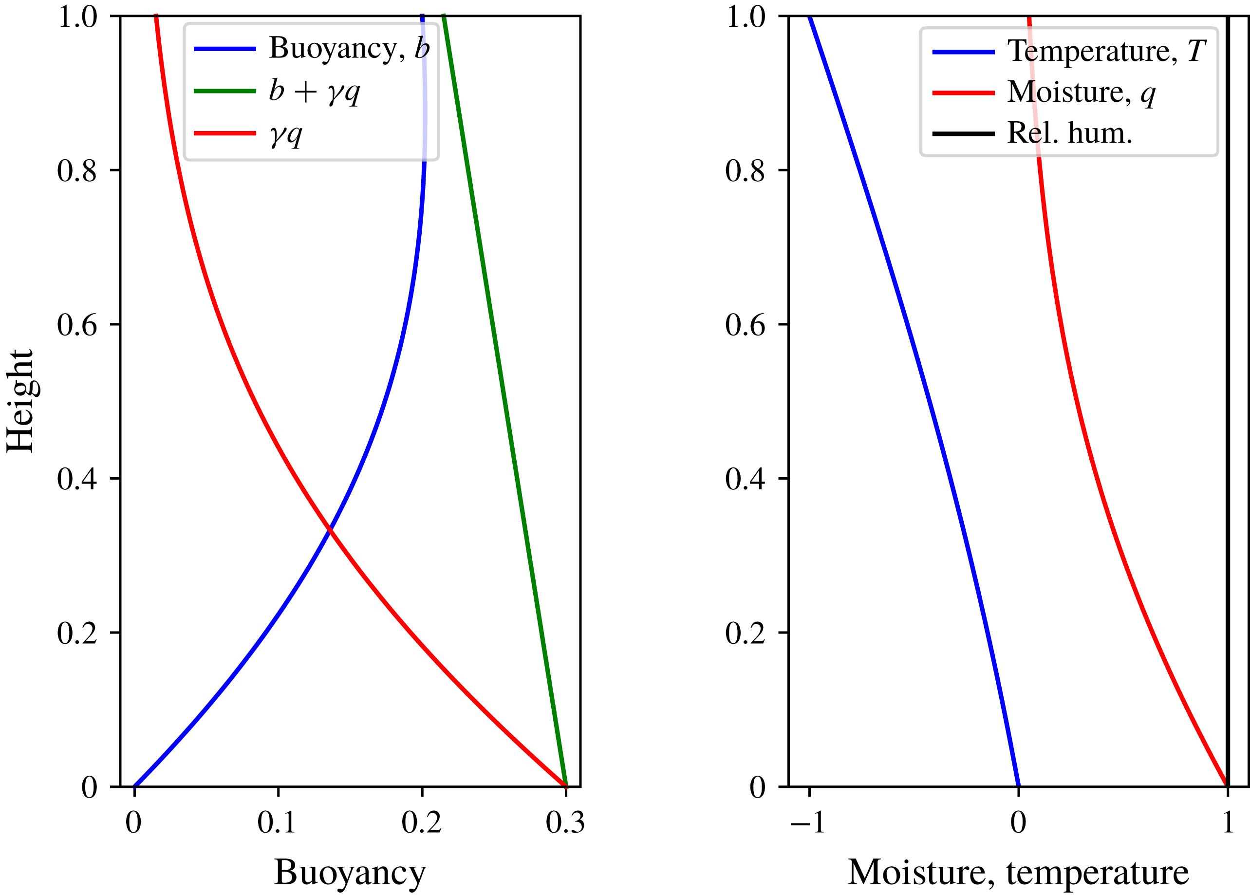
A non-dimensional drizzle solution with saturated upper and lower boundaries. The boundary conditions are that $b=0$ at $z=0$ and $b=0.2$ at $z=1$ and $q=q_{s}$ at both boundaries, thus giving the values of $m$ ( $=b+\unicode[STIX]{x1D6FE}q$ ) at the boundaries shown. These solutions were obtained with $\unicode[STIX]{x1D6FE}=0.3$ , $\unicode[STIX]{x1D6FC}=3$ and $\unicode[STIX]{x1D6FD}=1.2$ .

Figure 1 shows various profiles for buoyancy, temperature, humidity and $m(z)$ for a typical set of non-dimensional parameters. For this set of parameters, which is stable to dry convection, the buoyancy increases with height in the lower part of the domain, but decreases slightly in the top part of the domain. The variable $m(z)$ is linearly decreasing with height, implying that the solution will be unstable to moist convection in the diffusion-free limit. Finally, we remark that, at low Rayleigh number, numerical solutions of the nonlinear, time-dependent equations do converge to the drizzle solution.

5.2 Drizzle solution with unsaturated boundaries

In geophysical settings it is common to suppose that the lower boundary condition on moisture does not correspond to saturation; that is, the boundary – for example moist soil – is damp but not saturated; there will then be a layer of unsaturated air adjacent to the boundary. In the unsaturated layer the buoyancy and the moisture diffuse independently and each has a linear profile, but if the temperature falls off sufficiently rapidly with height then the water vapour will become saturated at some level, above which a solution similar to that of (5.6) holds.

Suppose that, as before, the boundary conditions at the bottom and top of the domain are ( $b_{1},q_{1}$ ) and ( $b_{2},q_{2}$ ) respectively, but that $q_{1}$ is less than the saturated value. The solution will be unsaturated below some height $z_{c}$ at which condensation begins, and for $0<z<z_{c}$ the profiles of both $b$ and $q$ are linear in $z$ , with no condensation. At $z_{c}$ the humidity takes its saturated value at $z_{c}$ and therefore $q_{c}=q_{s}(b_{c})=\exp [\unicode[STIX]{x1D6FC}(b_{c}-\unicode[STIX]{x1D6FD}z_{c})]$ . Above $q_{c}$ region is completely saturated and the calculation proceeds, in principle, as in the previous subsection, but with different boundary conditions and over the smaller domain. The height $z_{c}$ is determined by requiring that the first derivatives of temperature and moisture (as well as the values themselves) are continuous at the level of saturation, and this is most easily done numerically. That the first derivative should be continuous can be seen by integrating the governing equation across the condensation level giving

(5.14) $$\begin{eqnarray}\int _{z_{c}-\unicode[STIX]{x1D716}}^{z_{c}+\unicode[STIX]{x1D716}}\unicode[STIX]{x1D705}\frac{\unicode[STIX]{x2202}^{2}q}{\unicode[STIX]{x2202}z^{2}}\,\,\text{d}z=\int _{z_{c}-\unicode[STIX]{x1D716}}^{z_{c}+\unicode[STIX]{x1D716}}{\mathcal{H}}(q-q_{s})\frac{(q-q_{s})}{\unicode[STIX]{x1D70F}}\,\,\text{d}z.\end{eqnarray}$$

The right-hand side goes to zero as $\unicode[STIX]{x1D716}\rightarrow 0$ , even with the Heaviside function, and hence $\unicode[STIX]{x2202}q/\unicode[STIX]{x2202}z$ remains continuous, and similarly for temperature and buoyancy.

Figure 2.

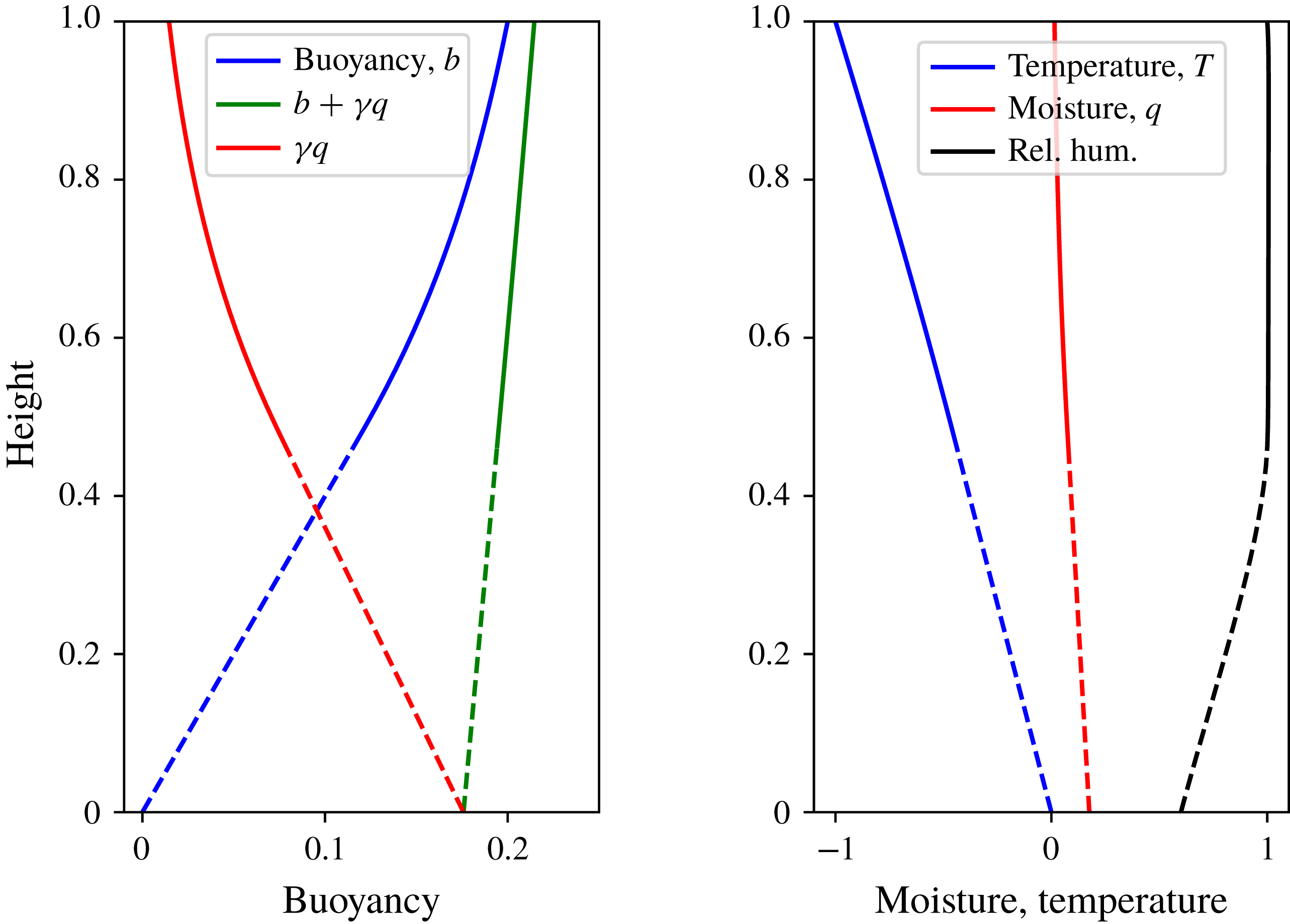
Drizzle solution with an unsaturated lower boundary, with relative humidity ( $q/q_{s}$ ) of 0.5. Other parameters are the same as in figure 1. The dashed lines show the linear profiles of moisture and buoyancy up to a height of approximately 0.45, above which the solution is saturated.

If the lower boundary is chosen to be saturated the solution is that described previously, whereas if the lower boundary is sufficiently dry then there is no condensation and buoyancy and moisture both vary linearly from bottom to top. A typical intermediate solution is illustrated in figure 2 with relative humidity equal to 0.6 at the lower boundary. Here the unsaturated region extends from the bottom to approximately $z=0.45$ over which the relative humidity increases monotonically until the air is saturated, above which the solution has a shape similar to that in figure 1, with the fields and their first derivatives remaining continuous throughout.

5.3 Stability of the drizzle solution

Figure 3.

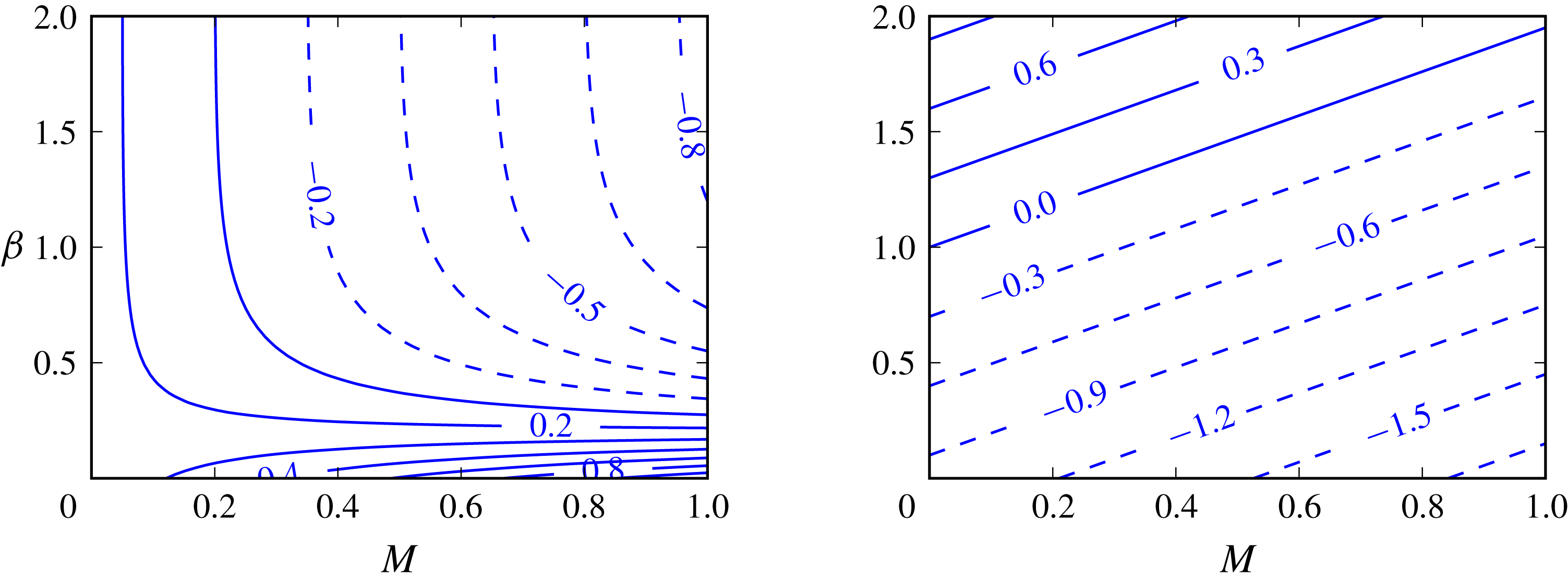
Contour plot of the value of the vertical gradient of $m(z)=b+\unicode[STIX]{x1D6FE}q_{s}$ (i.e. $\unicode[STIX]{x2202}m/\unicode[STIX]{x2202}z$ ) in the drizzle solution as a function of $\unicode[STIX]{x1D6FD}$ and $\unicode[STIX]{x1D6FE}$ , with $\unicode[STIX]{x1D6FC}=3$ . Panel (a) imposes values of $b(0)=0$ and $b(1)=0.2$ with $T=b-\unicode[STIX]{x1D6FD}z$ . Panel (b) has $T(0)=0$ and $T(1)=-1$ , with $b=T+\unicode[STIX]{x1D6FD}z$ . The boundary values of $q_{s}$ are calculated given the appropriate value of $T$ . Convective instability is possible in the region of dashed lines.

Figure 4.

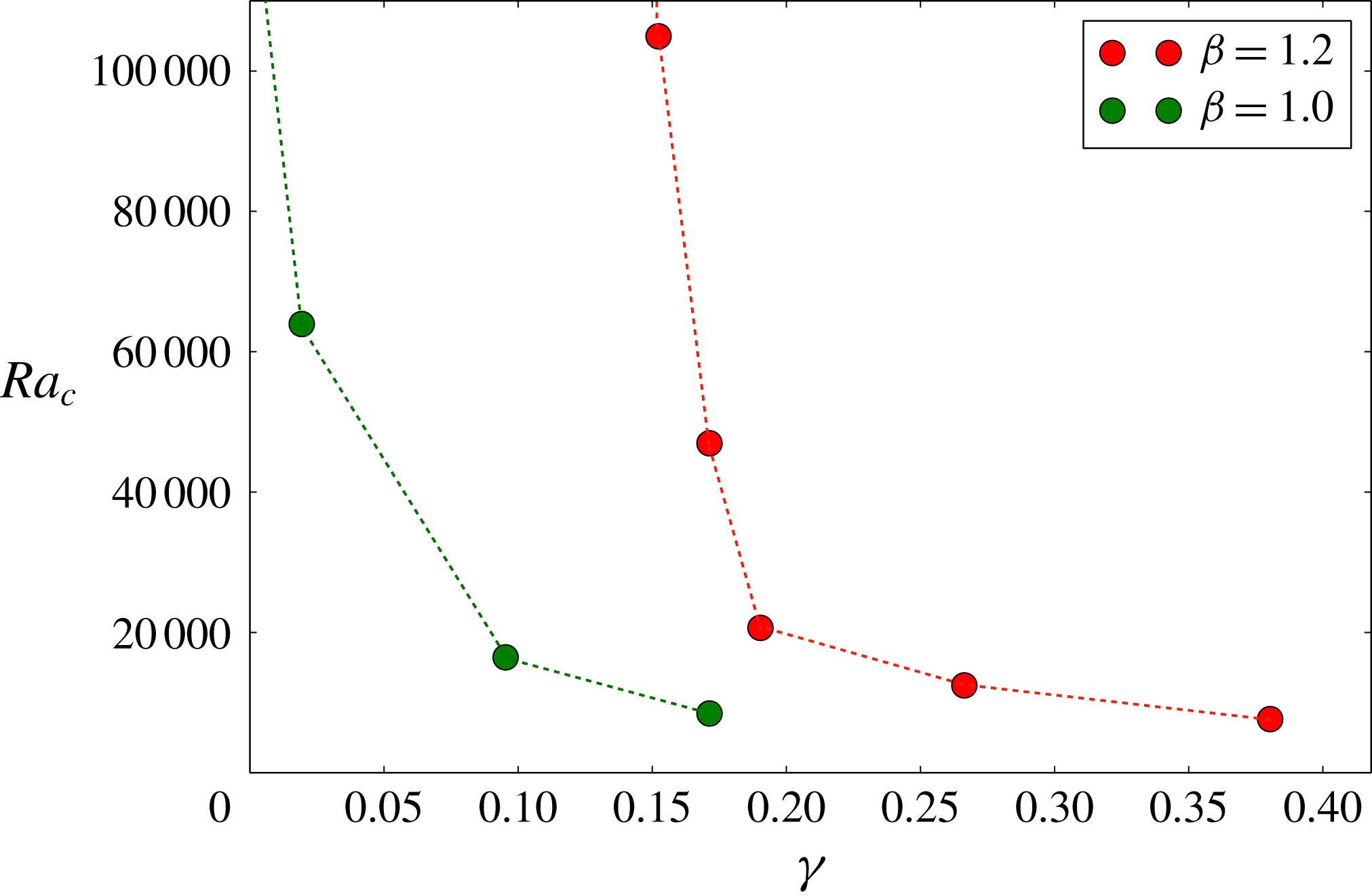
Stability of the linear drizzle solution. Graph of $Ra_{c}$ versus $\unicode[STIX]{x1D6FE}$ for the drizzle solution at $\unicode[STIX]{x1D6FD}=1$ (green) and $\unicode[STIX]{x1D6FD}=1.2$ (red). The dots mark the numerically determined stability boundary, with instability occurring above and to the right of the dots.

In the absence of diffusion the stability of the drizzle solutions is related to the sign of the gradient of the linear function $m(z)$ . Figure 3 gives the sign of this gradient as a function of the non-dimensional parameters $\unicode[STIX]{x1D6FE}$ and $\unicode[STIX]{x1D6FD}$ for the problem with saturated boundaries. As expected when $\unicode[STIX]{x1D6FE}=0$ (and moisture plays no role) stability is guaranteed if $\unicode[STIX]{x1D6FD}>1$ in the problem with specified temperature at the boundaries (right panel), and as $\unicode[STIX]{x1D6FE}$ is increased the critical $\unicode[STIX]{x1D6FD}$ for non-diffusive stability increases linearly with $\unicode[STIX]{x1D6FE}$ .

In the presence of diffusion, the stability of the drizzle solution is determined by $\unicode[STIX]{x1D6FE}$ , $\unicode[STIX]{x1D6FD}$ , $Ra$ and $\unicode[STIX]{x1D6FC}$ . Even for cases where instability is allowed in the non-diffusive case, instability in the diffusive cases only occurs for sufficiently high $Ra$ . The critical $Ra_{c}$ may be calculated by time-stepping from a slightly perturbed numerically calculated drizzle solution in a large domain followed by a bisection method. (The method thus strictly finds the stability with respect to small but not infinitesimal perturbations.) Figure 4 shows the critical Rayleigh number $Ra_{c}$ as a function of $\unicode[STIX]{x1D6FE}$ for two different choices of $\unicode[STIX]{x1D6FD}$ : $\unicode[STIX]{x1D6FD}=1.0$ corresponds to a neutrally dry marginally stable atmosphere and $\unicode[STIX]{x1D6FD}=1.2$ corresponds to a stable dry atmosphere, for the case with saturated boundaries. We see that $Ra_{c}$ approaches an asymptote at the non-diffusive threshold ( $\mathit{Ra}\rightarrow \infty$ ), and as $\unicode[STIX]{x1D6FE}$ is increased the critical Rayleigh number decreases. For $\unicode[STIX]{x1D6FE}=0$ the problem is that of dry convection and the case with $\unicode[STIX]{x1D6FD}=1.2$ is then always stable. The case with $\unicode[STIX]{x1D6FD}=1.0$ and $\unicode[STIX]{x1D6FE}=0$ will be stabilized by any non-zero diffusivity, and is neutrally stable in the infinite Rayleigh-number limit.

6.1 Variation with the Rayleigh number

Figure 5.

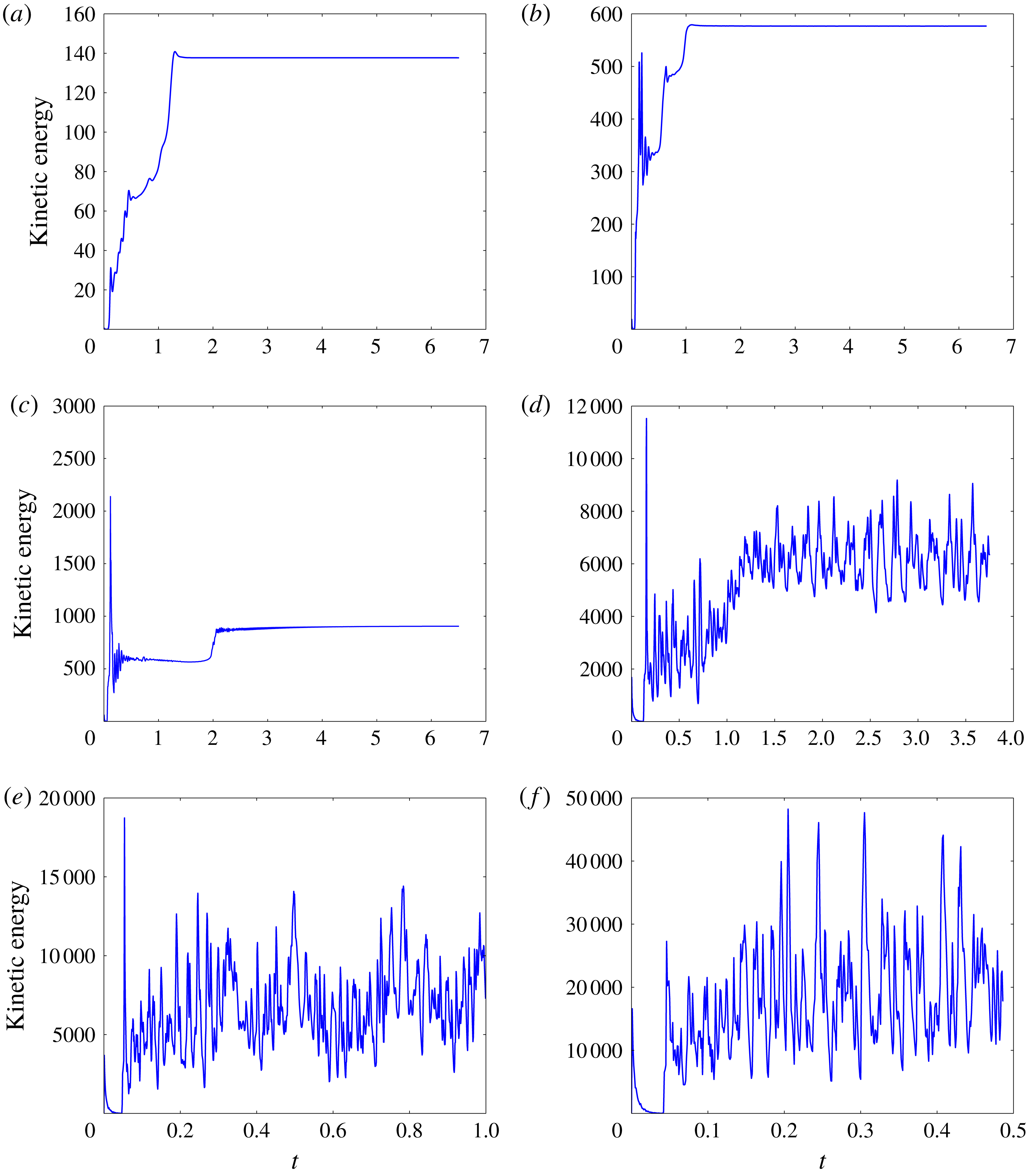
Time series for non-dimensional kinetic energy for numerical simulations with $\unicode[STIX]{x1D6FE}=0.19$ and (a) $Ra=2\times 10^{5}$ , (b) $Ra=1\times 10^{6}$ , (c) $Ra=2\times 10^{6}$ , (d) $Ra=2\times 10^{7}$ , (e) $Ra=5\times 10^{7}$ , (f) $Ra=2.5\times 10^{8}$ . The horizontal axis is time in diffusive units of $H^{2}/\unicode[STIX]{x1D705}$ , and note the differing scales of the axes in the panels.

In these experiments we vary the Rayleigh number but keep $\unicode[STIX]{x1D6FE}$ fixed, at $\unicode[STIX]{x1D6FE}=0.19$ . These parameters give the possibility of continued instability of the drizzle solution to moist convection for sufficiently high Rayleigh numbers, as can be seen from figures 3 and 4(b). The initial conditions are typically chosen so that $q=0$ in the interior of the domains except for a parcel of saturated air initially placed near the bottom boundary. This parcel immediately leads to heating and changes in the buoyancy field locally and triggers the start of moist convection. This initial condition naturally gives rise to plume triggering in the quiescent region of the domain before a statistically steady state is achieved, with the subsequent evolution depending on the Rayleigh number.

Figure 6.

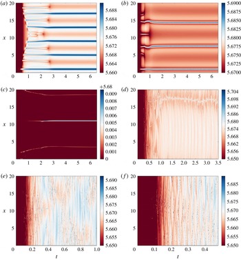
As for figure 5 but now time series (Hovmöller plots) at $z=0.5$ and for all $x$ for buoyancy for $\unicode[STIX]{x1D6FE}=0.19$ at (a) $Ra=2\times 10^{5}$ , (b) $Ra=1\times 10^{6}$ , (c) $Ra=2\times 10^{6}$ , (d) $Ra=2\times 10^{7}$ , (e) $Ra=5\times 10^{7}$ , (f) $Ra=2.5\times 10^{8}$ .

6.1.1 Time dependence and basic properties

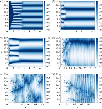
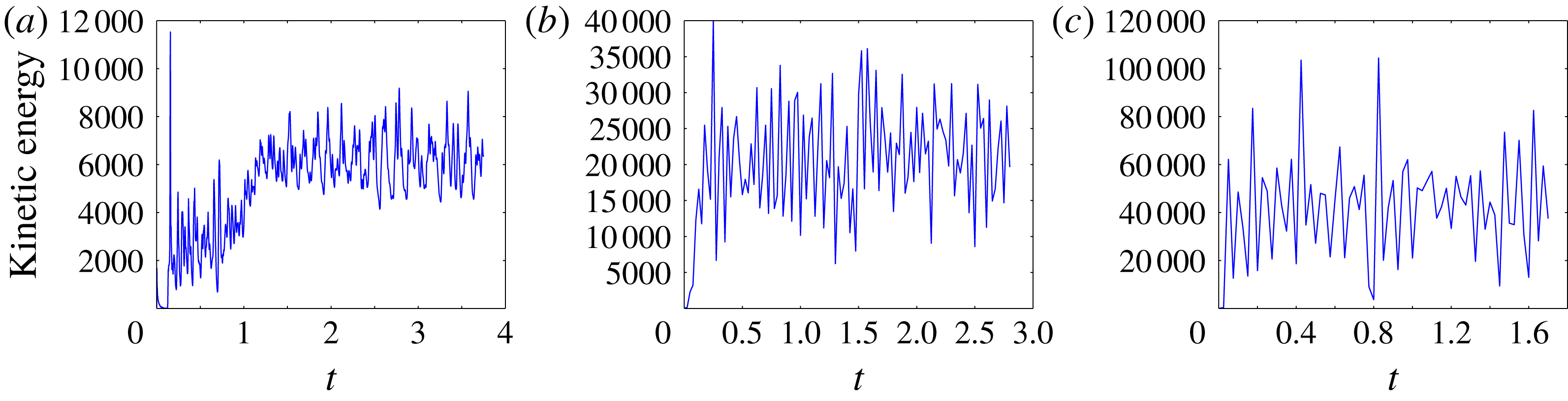
For small enough Rayleigh numbers (e.g. $Ra=10^{2}$ ) the action of diffusion damps out all motions and the system relaxes back to the drizzle solution, with saturation occurring everywhere in the domain. For high enough $Ra$ the drizzle solution is unstable to small perturbations and the trigger leads to sustained convection. Figure 5 gives time series of the kinetic energy for increasing $Ra$ , and figures 6 and 7 show the corresponding buoyancy and relative humidity evolution with time at $z=0.5$ and using Hovmöller plots (i.e. space–time plots showing a time series). For the three smallest values of $Ra$ the solution reaches a steady state and the kinetic energy approaches a constant value, which increases with $Ra$ . For the three higher values of the $Ra$ , the solution is unsteady and spatio-temporally modulated and as expected the average kinetic energy increases with $Ra$ . Irregular time dependence of solutions appears to arise more easily in moist convection than in dry convection, at least in two dimensions, because of the sharp nature of the nonlinearities expressed by the thresholds in moist convection.

Figure 7.

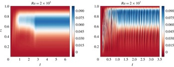
Time series (Hovmöller plots) for relative humidity ( $q/q_{s}$ ) at $z=0.5$ and for all $x$ for $\unicode[STIX]{x1D6FE}=0.19$ at (a) $Ra=2\times 10^{5}$ , (b) $Ra=1\times 10^{6}$ , (c) $Ra=2\times 10^{6}$ , (d) $Ra=2\times 10^{7}$ , (e) $Ra=5\times 10^{7}$ , (f) $Ra=2.5\times 10^{8}$ .

Figure 8.

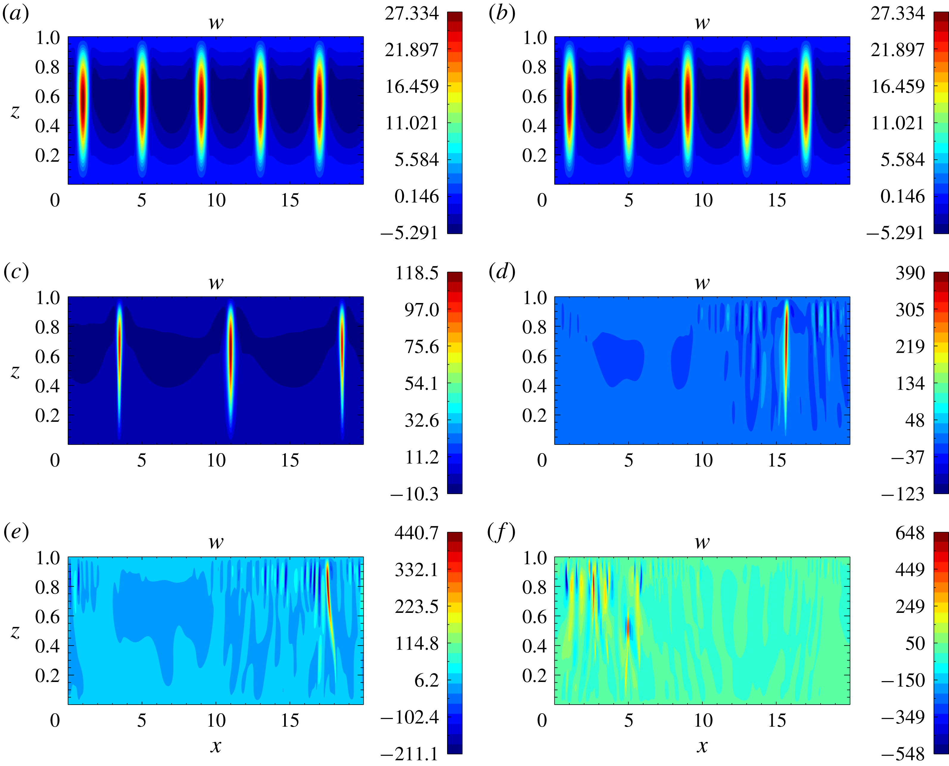
Snapshots of vertical velocity in a statistically equilibrated state for $\unicode[STIX]{x1D6FE}=0.19$ at (a) $Ra=2\times 10^{5}$ , (b) $Ra=1\times 10^{6}$ , (c) $Ra=2\times 10^{6}$ , (d) $Ra=2\times 10^{7}$ , (e) $Ra=5\times 10^{7}$ , (f) $Ra=2.5\times 10^{8}$ .

The nature of time dependence in the solutions can be seen in some of the movies that are included in the supplementary material available online at https://doi.org/10.1017/jfm.2018.954. Movie 1 shows the evolution from the initial conditions for the four variables, $b$ , $q$ , $T$ and $u$ , for $Ra=2\times 10^{5}$ . Initially the moist blob is seen in the $q$ field and rapidly heats the parcel causing a deficit in the buoyancy field that leads to its rise. This buoyant rise triggers gravity waves that advect the moisture field and thus triggers further buoyant patches to rise in the vicinity of the initial plume. This process continues until several (of the order of ten) buoyant plumes are found in the box. These plumes continue their evolution by sometimes merging and sometimes dying, until a steady state is reached with five equally spaced plumes in the box. The evolution is illustrated by Hovmöller plot of the buoyancy $b$ as a function of $x$ and $t$ for fixed $z=0.5$ , shown in figure 6(a). The diagram clearly shows the triggering of plumes at the beginning of the calculation followed by their merging and approach to a steady state. Figure 6(b,c) shows that the dynamics is similar for the next two smallest values of $Ra$ , but for $Ra=2\times 10^{6}$ there are only three plumes in the computational domain at the end of the calculation, with a wider spacing between plumes.

Movies 2–4 show the evolution for $Ra=2\times 10^{7}$ , $5\times 10^{7}$ and $2.5\times 10^{8}$ respectively. They show that the buoyant parcel rapidly triggers turbulent moist convection for these Rayleigh numbers. Here the plumes are much more time-dependent and for $Ra=2\times 10^{7}$ eventually the system is left in a state with a single, extremely time-dependent plume in the computational domain. This plume is very efficient at driving gravity waves, though for these parameters the waves are not instrumental in triggering plumes at other locations in the computational domain (as shown in figure 6 d). However as the Rayleigh number is increased multiple plumes are found in the domains, triggered by the gravity waves. These plumes are born and die rapidly as shown in the Hovmöller plots of figure 6(e,f). The triggering by the gravity waves for the turbulent solutions is most clearly seen in figure 7(d–f).

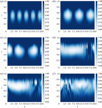
Figures 8 and 9 show snapshots of the spatial dependence of the solutions in a statistically equilibrated state for the vertical velocity ( $w$ ) and the relative humidity (defined as $q/q_{s}(T)$ ). For the steady solutions the solution takes the form of strong narrow updraughts surrounded by broader gentler downdraughts. The asymmetry is a well-known result in moist atmospheric convection (e.g. Ludlam Reference Ludlam1980), but in Boussinesq Rayleigh–Bénard convection the updraughts and downdraughts have exactly the same properties because of the up–down symmetry in the problem.

As the Rayleigh number is increased the updraughts become thinner and sparser and at high enough Rayleigh numbers they become unstable. For these higher Rayleigh numbers the plumes are extremely thin (and as noted earlier, very time-dependent). The relative humidity shows that for a moderate Rayleigh number the flow is saturated (red colour) in the updraughts and in the diffusive layers at the top and bottom of the computational domain. The downdraughts are in general not saturated since they are bringing dry air down into regions with higher temperatures where $q_{s}$ is larger, and the horizontally averaged relative humidity is a minimum in the domain interior, as discussed more below.

Figure 9.

Snapshots of relative humidity in a statistically equilibrated state for $\unicode[STIX]{x1D6FE}=0.19$ at (a) $Ra=2\times 10^{5}$ , (b) $Ra=1\times 10^{6}$ , (c) $Ra=2\times 10^{6}$ , (d) $Ra=2\times 10^{7}$ , (e) $Ra=5\times 10^{7}$ , (f) $Ra=2.5\times 10^{8}$ .

Figure 10.

Horizontally averaged profiles for (a) buoyancy and (b) $m(z)$ for $\unicode[STIX]{x1D6FE}=0.19$ and a range of $Ra$ .

6.1.2 Equilibrated properties

Equilibration of the moist convective solution is more complicated than in the dry problem. Roughly speaking, dry Rayleigh–Bénard convection equilibrates by mixing the buoyancy to an adiabatic profile in the core, thus effectively removing the driving except in thermal boundary layers at the top and bottom of the domain leaving the neutral profile, $\unicode[STIX]{x2202}b/\unicode[STIX]{x2202}z\approx 0$ , in the interior. In moist convection the analogous solution is a state corresponding to the saturated adiabatic lapse rate. In atmospheric models that cannot resolve convection, a simple convective parametrization is to adjust the buoyancy profile to satisfy these criteria, although adjustment methods are now commonly regarded as over-simple because the implied separation of time scales is too extreme (although improved parametrizations are hard to come by). To get a sense of the equilibration processes here we will show how various profiles vary as a function of Rayleigh number, with detailed analysis left for future work.

Figure 10 shows the horizontally averaged profiles in the statistically equilibrated state for the buoyancy and $m$ . Both are significantly modified by convection – recall that $m$ has a linear profile in $z$ in the saturated drizzle solution, which is reproduced only by the $\mathit{Ra}=1\times 10^{2}$ solution. The corresponding profiles in the upflows and downflows alone are shown in figure 11. These profiles show fairly uniform values of $m$ in the upper part of the domain, but the degree to which this is caused by mixing and/or adjustment through gravity waves in subsiding regions will be investigated in a subsequent paper. The lower part of the domain remains unstable even at high Rayleigh number (see also figure 18 c), and whether this result holds at still higher Rayleigh number, and in three dimensions, is also a topic for future investigation. The buoyancy fluxes giving rise to these profiles are shown in figures 12 and 13. In both the steady and unsteady cases the buoyancy flux is peaked in the upper half of the domain, in fact close to the diffusive upper boundary layer in the unsteady case. The moisture flux (not shown) peaks lower down, largely because there is much more moisture where the temperature is higher.

Figure 11.

(a,b) Averages taken over the upflows alone (where $w>0$ ) of (a) the buoyancy and (b) the moist static energy, $m$ . (c,d) The same, except that averages are taken over downflows alone (where $w<0$ ).

Figure 12.

Time and horizontally averaged vertical buoyancy flux, $\langle w^{\prime }b^{\prime }\rangle$ , at two values of Rayleigh number. Note the peak flux rising up to the top boundary layer at higher Rayleigh number. The time series of these fields are shown in figure 13.

Figure 13.

Time series (Hovmöller plots) of the $x$ -averaged buoyancy fluxes $\langle w^{\prime }b^{\prime }\rangle$ at each height, at two values of Rayleigh number. The time-averaged fields, over the later parts of the time period, are shown in figure 12.

Figure 14.

(a) Kinetic energy as a function of $Ra$ . (b) Area fraction of near-saturated upflows as a function of $Ra$ , with three different criteria. The blue line requires $w>0$ and $RH>0.95$ , the green line requires $w>0.02w_{max}$ and $RH>0.95$ and the red line requires $w>0.1w_{max}$ and $RH>0.95$ .

Figure 14 shows the kinetic energy and the fraction of the domain covered by near-saturated upflows as a function of $Ra$ . As expected (at least for moderate values of Rayleigh number, and given that the Reynolds number is often taken to be the square root of the Rayleigh number) the kinetic energy increases with $Ra$ . The area fraction of upflows has a more complicated dependence, and depends on the criterion used. For the steady solutions (the lowest three values of $Ra$ ) the area fraction actually decreases with $Ra$ if the weakest criterion ( $w>0$ ) is used. As $Ra$ is increased further the solutions become time-dependent and the area fraction of upflows stays roughly constant – the strong upflows are very narrow, but there are a greater number of weak upflows. However, this criterion is most likely picking up flows with positive vertical velocity due to gravity waves and not associated with updraughts, and this V-shaped dependence is in fact reproduced without any restriction on relative humidity. With the more restrictive criteria (red and green lines in the figure) the upflow fraction decreases and then seems to converge to a definite value as Rayleigh number increases, with the structures generally remaining space filling. Understanding the parameter dependence of these results, and whether there is any universality, is of direct relevance to meteorology, since ‘mass flux parametrization schemes’ commonly used in coarse resolution atmospheric models often assume that updraughts occupy some fixed fraction of the domain.

Figure 15.

Horizontally averaged relative humidity over a range of Rayleigh numbers, with all other parameters fixed.

Figure 16.

Scatter plots of relative humidity, $RH$ , and vertical velocity, $w$ , over a range of Rayleigh numbers, as labelled. Note the changes in the scale of the $x$ -axis.

6.2 Variation with condensational parameter, $\unicode[STIX]{x1D6FE}$

Figure 17.

Time series for kinetic energy at $Ra=2\times 10^{6}$ for (a) $\unicode[STIX]{x1D6FE}=0.19$ , (b) $\unicode[STIX]{x1D6FE}=0.38$ and (c) $\unicode[STIX]{x1D6FE}=0.76$ . Note the different scales on the vertical axes.

We now focus on the role of the (non-dimensional) condensation parameter $\unicode[STIX]{x1D6FE}$ , with other parameters fixed. As discussed earlier, changing $\unicode[STIX]{x1D6FE}$ modifies the stability of the drizzle solution (as shown in figure 3). For fixed $\unicode[STIX]{x1D6FD}>1$ and small $\unicode[STIX]{x1D6FE}$ the drizzle solution will remain stable whatever the value of $Ra$ . As $\unicode[STIX]{x1D6FE}$ is increased the gradient of $m(z)$ is altered until it becomes negative and instability occurs if the Rayleigh number is sufficiently high. We thus conduct a series of experiments for moderately high $Ra$ ( $Ra=2\times 10^{6}$ ) and with all other parameters as before, and vary $\unicode[STIX]{x1D6FE}$ . For $\unicode[STIX]{x1D6FE}\lesssim 0.13$ the drizzle solution is linearly stable for all $Ra$ . Numerical solutions in fact indicate that for $\unicode[STIX]{x1D6FE}\lesssim 0.13$ the solution always returns to the drizzle solution. As $\unicode[STIX]{x1D6FE}$ is increased further, steady then unsteady nonlinear solutions are found, and time series of the kinetic energy for $\unicode[STIX]{x1D6FE}=0.19$ , 0.38 and 0.76 are shown in figure 17. As expected, as $\unicode[STIX]{x1D6FE}$ is increased the kinetic energy of solutions increases, appearing to scale roughly linearly with $\unicode[STIX]{x1D6FE}$ for large $\unicode[STIX]{x1D6FE}$ .

Figure 18 shows the effect of varying $\unicode[STIX]{x1D6FE}$ on the mean profiles of buoyancy, relative humidity and $m$ . As the heating is increased (by increasing $\unicode[STIX]{x1D6FE}$ ) the buoyancy of the layer is increased and the relative humidity decreased. The net effect is to increase $m$ , with $m$ being well mixed between $z=0.5$ and a thin boundary layer near to the top of the domain. The lower half of the domain remains convectively unstable (as noted earlier), and whether it becomes neutralized at higher values of the Rayleigh number is a topic for future investigation.

We conclude with a remark on subcritical convection – i.e. sustained convection occurring for $Ra<Ra_{c}$ , where $Ra_{c}$ is the critical Rayleigh number at which the linear instability of the drizzle solution occurs. No such behaviour has been found for this two-dimensional model for an aspect ratio of 20, suggesting global (nonlinear) stability for this configuration. On the other hand, Pauluis & Schumacher (Reference Pauluis and Schumacher2011) and Weidauer, Pauluis & Schumacher (Reference Weidauer, Pauluis and Schumacher2011) did appear to find occurrences of sustained convection in a regime they deemed subcritical by a different criterion and in a different system from ours. Pace their results, we are unable to say whether sustained subcritical convection is a general property of moist convection.

Figure 18.

Horizontally averaged profiles for (a) buoyancy, (b) relative humidity and (c) $m(z)$ for $Ra=2\times 10^{6}$ and a range of $\unicode[STIX]{x1D6FE}$ . Note the different horizontal scale for $\langle m\rangle$ from those of earlier figures showing $\langle m\rangle$ .