2.1. The visual mechanism of flying insects

Honeybees are species of compound-eye insects. These compound eyes are composed of tens of thousands of ommatidia and the most obvious advantage of the ommatidium is that flying insects can effectively calculate the relative positions and distances from themselves to the observed objects, and then make their own judgments and response quickly. The observed range of each ommatidium is very narrow and the observed scenes overlap with each other between the adjacent ommatidia. The entire scene observed by all the ommatidia forms a panoramic image. Unlike vertebrates, flying insects cannot infer the distances to objects or surfaces due to their immobile eyes with fixed-focus optics. Thus they fall back on image motion, induced by their own motion, to deduce the distances to obstacles and to control various manoeuvres [Reference Wehner7,Reference Srinivasan, Lehrer, Kirchner and Zhang10].

Research on the orientation performances of honeybees has agreed that honeybees determine the direction of the food source by using the sun compass, but there still exists controversy with respect to the possible cues used to measure the distance to the food source. Karl von Frich [Reference von Frisch13] proposed a theory of “energy hypothesis” that the honeybees infer the distance to the food source by measuring the amount of energy spent on the foraging trip. However, recent studies have discovered a number of different ways in which honeybees use visual cues for navigational purposes [Reference Wehner7,Reference Srinivasan, Lehrer, Kirchner and Zhang10,Reference Baird, Srinivasan, Zhang, Lamont and Cowling11]. At the same time, some evidence has confirmed that the flight speeds of flying insects are regulated by monitoring the velocity of the image through their retinas [Reference David14,Reference Baird, Srinivasan, Zhang and Cowling15]. Some findings [Reference Esch, Zhang, Srinivasan and Tautz16] have proved that the distance is indeed estimated in terms of the total extent of image motion that is experienced by the eyes en route to the destination.

2.2. The concept of entropic map

2.2.1. Entropy

A theoretical approach to information is based on the concept of entropy introduced by Shannon in information theory [Reference Shannon17]. Suppose that a source X has L source alphabets and the probability of the i-th source x _i is given by p _i, where p _k⩾0 (k=1, 2, …, L) and ∑p _k=1. An effective means to describe the information for the source X is the mean of self-information over the L source alphabets, which is called Shannon entropy.

(1)

As an image is viewed as an information source with a probability vector described by its histogram L of the image I, the entropy of the histogram can be used to represent a certain level of information contained in the image. The entropy of an image is a scalar and it represents the total information content contained in the image.

2.2.3. The concept of entropic map

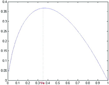
The graph of function y=−xlogx is shown in Figure 1. The function has a maximum point 1/e and it has two monotone intervals. These properties result that the contrast of the local entropic map is often out of accord with the original image. If the variable x is multiplied by 1/e, the function will be limited to the interval [0, 1/e] and increase monotonically in the interval [0, 1/e], which is valid to avoid altering the contrast of the image. At the same time, the grey value f(i, j) at the point (i, j) can be interpreted as the number of photons arriving at that point. If the total number of photons is viewed as 1, the grey value f(i, j) will be interpreted as the probability distribution of photons, i.e. p(i, j). According to these opinions, the choice of p(i, j) in our entropic map is described as:

(2)

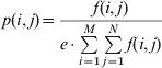
where f(i, j) expresses the grey value at the point (i, j) and M×N means the size of the whole image.

Figure 1.

The graph of function y=−xlogx.

In constructing the entropic map, the segmented method simulates the principle of compound eyes of flying insects. For an image of size M×N, the constructing algorithm of entropic matrix T is described as follows:

1. (1) Calculate p(i, j) at each point (i, j) according to equation (2);

2. (2) Partition the image into equal-sized rectangular sub-blocks (the number of blocks is P×Q), and the adjacent sub-blocks will share a certain percentage of overlapping;

3. (3) Compute entropy H _ij (1⩽i⩽P, 1⩽j⩽Q) of each sub-block according to equation (1);

4. (4) Use all sub-blocks of entropy to form an entropic matrix T.

The entropic matrix T is shown

(3)

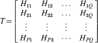
If the entropic matrix T is normalized via the linear normalization method, the entropic map will be established. The entropic map can characterize topographic features of an image and its accuracy is relative to the fine grit of the sub-block.

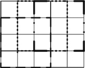
In this paper, the original image is divided into blocks of size 3×3 and the overlapping ratio between two horizontal and vertical adjacent blocks is 2/3. The diagram of the intersected method is shown in Figure 2.

Figure 2.

The diagram of intersected method.

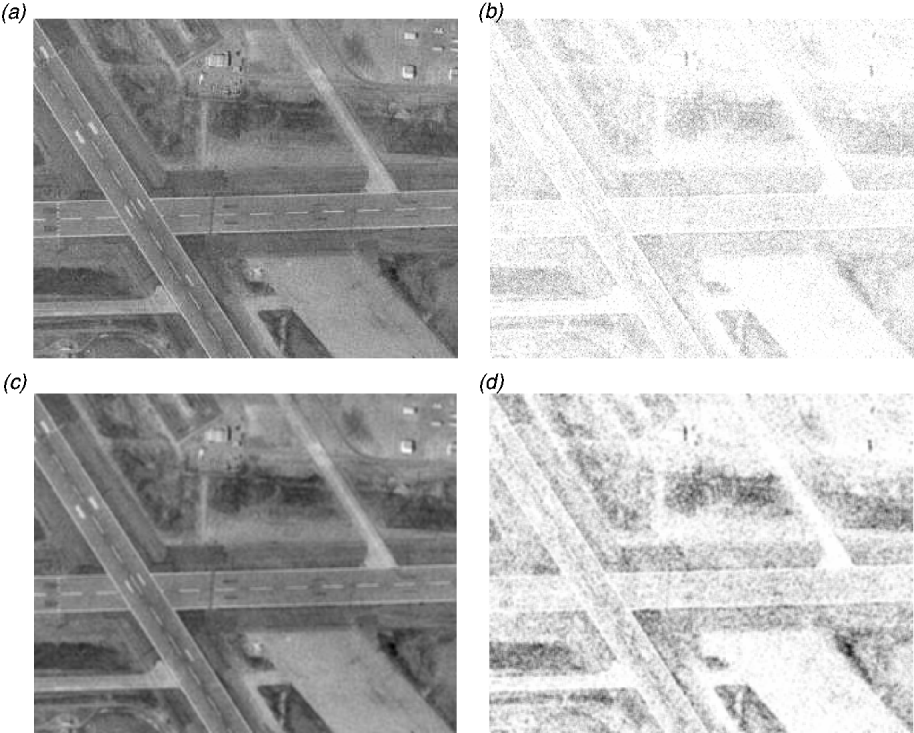
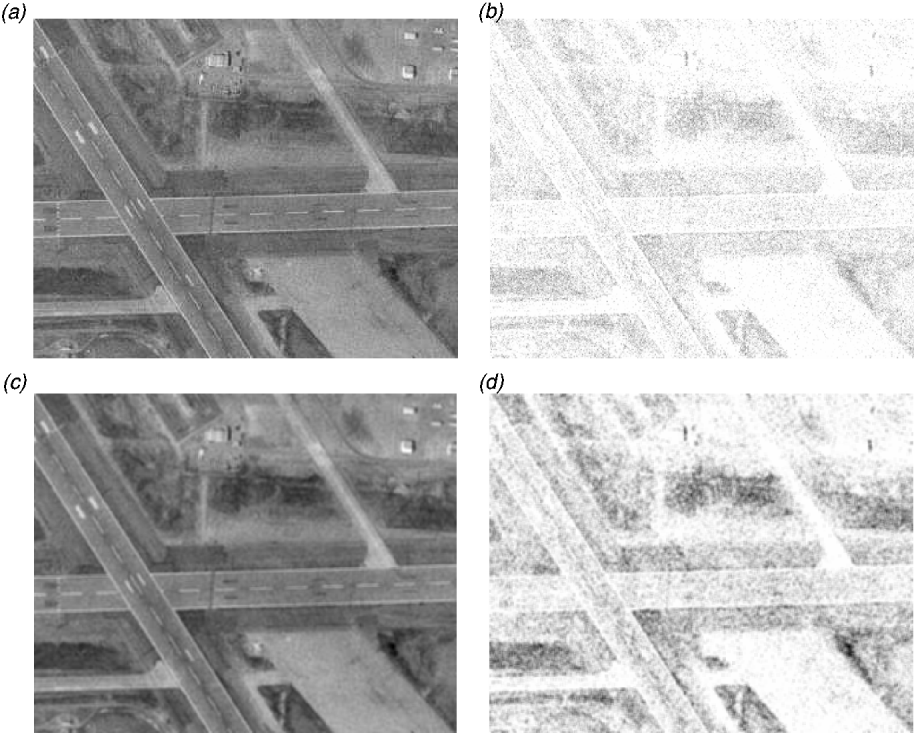
Figure 3 (a) is an original airport image, and we have added Gaussian noise with zero mean and variance var=0·5 to it, as shown in Figure 3 (b). Their corresponding entropic maps are shown in Figure 3 (c) and (d) respectively (via normalization). From Figure 3, we can see that entropic maps are insensitive to noise, similar to low-pass filter.

Figure 3.

(a) Top left: Original airport image. (b) Top right: The image degraded by Gaussian noise with var=0·5. (c) Bottom left: Entropic map corresponds to the original image. (d) Bottom right: Entropic map corresponds to the noise image.

2.3. Entropy flow

2.3.2. The computation of entropy flow

Optical flow is an approximate descriptor of image motion. Starting with the classical works of Horn and Schunck [Reference Horn and Schunck20] as well as Lucas and Kanade [Reference Lucas and Kanade21], there are tremendous computational methods of optical flow. Barron et al. [Reference Barron, Fleet and Beauchemin22] suggested that the phase-based technique of Fleet and Jepson [Reference Fleet and Jepson23] and the differential technique of Lucas and Kanade [Reference Lucas and Kanade21] produced the more accurate results overall. Galvin et al. [Reference Galvin, McCane, Novins, Mason and Mills24] concluded that the technique developed by Lucas and Kanade yields the best results.

In order to analyze motion within subsequent frames of an image sequence, temporal constancy has to be imposed on certain image features. The most frequently used feature in this context is the image brightness, i.e. the grey values of image objects in subsequent frames do not change over time. The brightness constancy assumption is also accepted to compute entropy flow in this paper, which makes the instantaneous entropy value in an entropic map sequence stay unchanged over time:

(4)

where the displacement field v=(u, v)^T(x, y, t) is entropy flow. For small displacements, we may perform a first order Taylor expansion to yield the entropy flow constraint (EFC):

(5)

where subscripts denote partial derivatives. It is evident that this single equation is not enough to uniquely compute the two unknowns u and v (aperture problem).

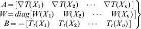
For the solution of equation (5), we add a local constant model to v, similar to Lucas and Kanade [Reference Lucas and Kanade21]. Assume that in a small neighbourhood space Ω, the motion vectors remain constant, then the entropy flow can be estimated through weighted least-squares method. In a small spatial neighbourhood Ω, the estimation of entropy flow is computed by minimizing

(6)

where W(x,y) represents a window. Then the solution of u and v is as follows

(7)

where in the time t, X _i Ω and

(8)

2.3.3. The performance evaluation of entropy flow

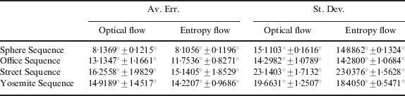
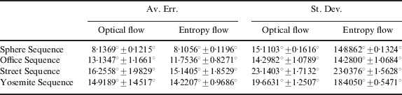
Entropy flow is also an approximation of image motion. We compare entropy flow with optical flow in the estimated performance of image motion for four synthetic image sequences, since their 2-D image motion fields are known. In computation of optical flow, temporal smoothing is usually needed to avoid aliasing, but numerical differentiation must be done carefully [Reference Beauchemin and Barron25]. In this paper, a Gaussian smoothing kernel with standard deviation σ=1 is used in the computation of optical flow, while that process is not necessary in calculation of entropy flow since the entropic map is robust to noise from section 2.2.

Three synthetic sequences, i.e. sphere sequence, office sequence and street sequence, are available from www.cs.otago.ac.nz/research/vision/ while the fourth sequence, Yosemite without clouds sequence is available from http://www.cs.brown.edu/people/black/images.html. The qualitative performance of image motion field is authenticated by the quantitative evaluations, i.e. measuring in terms of the error measure [Reference Fleet and Jepson23], namely the angular error between the correct image motion (u _c, v _c) and the estimated motion (u _e, v _e) via

(9)

where ϕ _e is the angular error. The comparisons between entropy flow and optical flow was by means of average angular error (Av. Err.) and standard deviation of angular error (St. Dev.). The average angular errors and their standard deviations of four synthetic image sequences are shown in Table 1. It suggests that the estimation performance of entropy flow as a whole surpasses that of optical flow from Table 1. The reason may be that entropy flow possesses a bionic property since it is based on the visual mechanism of the flying insects, so it yields more precise results.

Table 1.

The averages and standard deviations of angular errors for four synthetic image sequences.

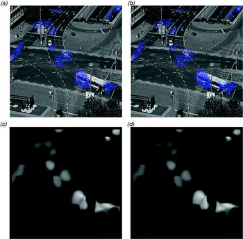
The comparisons for realistic image sequence Ettlinger Tor Traffic sequence are shown in Figure 4. This sequence is available from http://i21www.ira.uka.de/image_sequences/, and it consists of 50 frames of size 512×512. The computed entropy flow and optical flow field, as well as their corresponding magnitudes of flow field are shown in Figure 4. It suggests that entropy flow is very approximate to image motion, and perhaps it is better in depicting performance of image motion.

Figure 4.

(a) Top left: Computed entropy flow field between frame 24 and 25. (b) Top right: Computed optical flow field. (c) Bottom left: The magnitude of entropy flow field. (d) Bottom right: The magnitude of optical flow field.

3.1. Six-parameter affine motion model

The field generated by the 3-D rigid object motion is projected onto a 2-D motion field under the orthogonal projection which can be depicted by both affine motion model and non-linear perspective motion model. With regard to global motion models, we adopt a six-parameter affine motion model because of its reasonable trade-off between complexity and accuracy. The basic form of six-parameter affine motion model is described as:

(10)

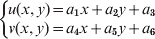
where v=(u(x, y), v(x, y)) represents the motion at the point (x, y). If we assume α_u^T=(a ₁, a ₂, a ₃), α_v^T=(a ₄, a ₅, a ₆), X=[x, y, 1], we will get u(x, y)=X·α_u and v(x, y)=X·α_v. Obviously, when the motion v is known, the parameters α_u and α_v will be estimated through a least-squares estimation algorithm because of its small computational complexity and good estimated accuracy. Then the solution of a ₁, a ₂, a ₃, a ₄, a ₅, a ₆ is as follows:

(11)

where D is a set of points in the entropic map.

3.2. Auto-selecting algorithm of assessment threshold

However, the estimated uncertainty and the violation of EFC have a great impact on the estimated accuracy of those motion parameters. In order to improve computational accuracy and efficiency of global motion estimation, an auto-selecting algorithm of assessment threshold is proposed in this paper. From equation (10), three motion vectors v are enough to solve those motion parameters. But this strategy is not adopted because of large errors. The method that all motion vectors v contribute to compute the motion parameters is also inadvisable owing to the volatility of entropy flow and bulky calculated amount. The aim of the auto-selecting algorithm of assessment threshold is to seek a small quantity of entropy flow with little volatility. Therefore, the entropy flow field is divided into sub-blocks of equal size, and the motion parameters are estimated in each sub-block. The estimated parameters in each sub-block are shown as:

(12)

where α_ui^T and α_vi^T denote the estimated parameters in i-th sub-block, D _i is a set of points in i-th sub-block, and M is the number of sub-blocks.

In order to evaluate the estimated performances of these sub-blocks, the estimated error is introduced in this paper. The estimated error of each sub-block is defined as:

(13)

where N _i is the number of points in i-th sub-block, v_i is the original entropy flow in i-th sub-block, v_ai is the estimated entropy flow through estimated motion parameters, and M is the number of sub-blocks. Then, some sub-blocks whose estimated errors are small via a threshold are chosen to re-estimate the motion parameters, which may result in more accurate motion parameters and smaller calculated amount.

The selection of threshold is very important. In our simulation experiments, we found that the proportion of block selection has a great effect on the threshold. The auto-selecting algorithm of assessment threshold is based on the proportion of block selection, and described in detail as follows:

1. (1) Partition the entropy flow field into sub-blocks of equal size (the size usually is 8×8 or 16×16);

2. (2) Calculate estimated errors of each sub-block, σ_i², i=1, 2, …, M, and M is the number of sub-blocks;

3. (3) Set up an initial threshold Ω=Ω₀ and the step length ΔΩ;

4. (4) Choose the sub-blocks whose estimated error satisfy σ_i²⩽Ω, i=1, 2, …, N, where N means the number of selected sub-blocks;

5. (5) Put up the proportion of block selection β, if N/M ⩾β, then Ω is the final threshold. Otherwise, Ω=Ω+ΔΩ, return to Step 2 and continue to search.

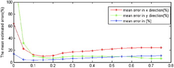
The respective mean of estimated errors of the translation in X, Y and Z coordinates are shown in Figure 5 (the block size is 16×16). The horizontal axis represents different proportion of block selection β and the vertical axis denotes the mean estimation error (the errors are described in percent). The total number of experiments is 288 and β is finally chosen as 0·15 in the following work.

Figure 5.

The respective mean errors under different proportions of block selection.

4.1. Kalman filter

The least-squares estimation algorithm is adopted to estimate the parameters of global motion. However, the least-squares algorithm is usually more sensitive to data noise. It is a linear minimum deviation estimation and its process needs to know the first-order and the second-order moments of the estimator exactly, which is very harsh, usually impossible for a non-stationary process. Therefore, the estimated results have a certain extent of error and need to be amended.

In the 1960s, the Kalman filter method [Reference Kalman26] was proposed, which aroused worldwide application. The advantage is that it has transitivity, so it does not store large amounts of historical information and can reduce the amount of storage in the computer, directly combining the system state equation with observation equation, and estimating parameters of the system state while directly giving estimated accuracy. So it is widely used in process control, telecommunications and biomedical fields, etc.

4.2. The framework of the navigation algorithm

The novel navigation algorithm is modelled on the basis of the navigation mechanism of particular flying insects – honeybees. From section 2.1, the flight direction of honeybees to the food source is definite since they determine the direction by using the sun compass, which rouses us to plan the flight path of the missile beforehand (called reference trajectory). Meanwhile, honeybees use cues of image flow induced by their own motion to avoid lateral obstacles, to control their speed and height, to cruise and land, which inspires us to fix a high-performance camera on the abdomen of the missile. The aim of the camera is to snap the real-time image sequence and then expect to regulate the flight trajectory of the missile in real time (called real-time trajectory). Furthermore, the motion parameters of the camera, i.e. the real-time flight regime of the missile, are estimated through entropy flow, and then a series of aerial photographs from an original point (location) to the target point (location) are stored in the missiles beforehand (called reference image sequence). Under the above initial assumptions, the control system of the missile may continuously modulate its control signal to regulate the flight trajectory of the missile through the navigation algorithm based on the entropy flow and a Kalman filter, to reach the goal.

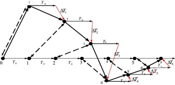
The computation of entropy flow is between real-time images and their corresponding reference images, rather than only in the reference image sequence or the real-time image sequence. The initial image in the reference image sequence is viewed as the first-frame image, while the initial image in the real-time image sequence is regarded as the corresponding second-frame image. Then the entropy flow filed will be calculated according to section 2, and the motion parameters of the missile are obtained based on section 3. The control system of the missile regulates the trajectory, and instructs the missile to reach the next target point (location). By repeating that process, the missile will arrive at the end-point. The navigation algorithm is a continuously iterative process to ensure arrival at the end-point. The sketch map of the navigation algorithm is shown in Figure 6.

Figure 6.

The sketch map of the navigation algorithm.

In Figure 6, 0, 1, 2, …, 6, … represent the respective positions of the reference trajectory and they move in a unit time to reach the next position according to the scheduled speed and direction (i.e. T ₀). The images in the position 0, 1, 2, …, 6, … are viewed as the first frame, the second frame,..., the sixth frame, … in the reference trajectory, i.e. reference images. These images are converted into the entropic maps, which are denoted as 0, 1, 2, …, 6, … respectively. 1′, 2′, …, 6′, … represent the positions of the real-time trajectory and they move in a unit time to arrive at the next location according to the amendatory speed and direction (i.e. T ₀+ΔT ₁, T ₀+ΔT ₂, …, T ₀+ΔT ₆, …). The following work is similar to the above, denoted as 1′, 2′, …, 6′, … respectively.

The navigation algorithm based on the entropy flow and Kalman filter is described in detail as follows:

1. (1) Compute entropy flow between 1′ and 0 according to section 2;

2. (2) Estimate the motion parameters of the missile in the light of section 3;

3. (3) Input the estimated parameters to Kalman filter to obtain the optimized motion parameters ΔT ₁;

4. (4) The position of 1′ moves to the position of 2′ through T ₀+ΔT ₁.

The translation in X and Y coordinates can be viewed as the velocity in X and Y coordinates since we only consider the displacements in X, Y and Z coordinates in a unit time interval in this paper. Return to step 1, and compute entropy flow between 2′ and 1, the optimized parameters ΔT ₂ will be obtained, thus the position of 3′ is available by 2′ moving T ₀+ΔT ₂. Repeat the above steps, therefore a series of rectification ΔT ₃, ΔT ₄,…will be obtained respectively until arriving at the goal.

5.1. Simulation process

The reference images were snapped in five different initial locations at seven different heights, and the central positions of their images were controlled by the latitude and longitude in Google Earth, i.e. (30°30′35·03″,114°24′29·04″), (23°09′36·36″,113°14′58·45″), (30°30′20·22″,114°24′44·24″), (39°54′18·16″, 116°24′27·74″), (40°39′10·33″,73°57′34·33″). At each central location, seven images were snapped respectively, from the height of 1850m to 2150m, with 50m as an interval. The total number of snapped images was 35 and the size was 689×1024. The snapped images in different view heights were used for simulating the changes of the height, and forming other images which are in the other height through an interpolation algorithm in simulation experiments.

During the practical flight, random error is inevitable. In order to simulate random error, in the fourth step of the navigation algorithm in section 4.2, we have added random errors in the interval [−0·5, 0·5] (unit: pixel) on the translations in X and Y coordinates and random errors in the interval [−5, 5] (unit: metre) on the translation in Z coordinate in each iteration step. The initial location of the real-time trajectory is obtained from the initial position of reference trajectory where an initial error is added.

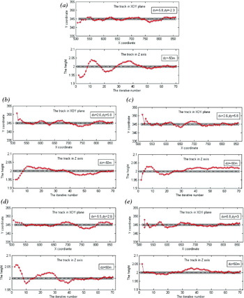
The simulation experiments at each initial position accompanied by five different initial errors are repeated 30 times randomly, then the total number of simulation experiments is 750. Five experimental results randomly singled out from five different initial positions are shown in Figure 7. Each image has two sub-images. The real-time amendatory trajectory in the XOY plane is shown in the first sub-image, where the red curve with volatility is the real-time trajectory and the grey line in the centre represents the reference trajectory. The real-time amendatory trajectory in the Z axis is shown in the second sub-image, where the red curve with volatility is the real-time modified height and the grey line in the centre is the reference height 2000m. The initial errors in X and Y coordinates were (−5·8, −2·3), (2·6, 5·8), (2·6, 5·8), (−5·5, 2·6), and (6·8, 3·0) respectively (unit: pixel), while the respective initial errors in Z axis were 50m, −50m, 50m, 50m and 50m (unit: metre).

Figure 7.

(a) Top: A result randomly taken out from (30°30′35·03″, 114°24′29·04″) and its initial error is (−5·8, −2·3, −50). (b) Middle left: From (23°09′36·36″, 113°14′58·45″) and the initial error is (2·6, 5·8, −50). (c) Middle right: From (30°30′20·22″, 114°24′44·24″) and the initial error is (2·6, 5·8, −50). (d) Bottom left: From (22°39′06·36″, 113°29′58·45″) and the initial error is (−5·5, 2·6, 50). (e) Bottom right: From (36°39′55·19″, 116°59′41·69″) and the initial error is (6·8, 3·0, 50).

5.2. Circular error probability (CEP)

In the military science of ballistics, circular error probable (CEP) or circular error probability is an intuitive measure of testing a weapon system's accuracy. In Pitman [Reference Pitman27], CEP is defined “as the radius of a circle around a target for which there is a 50% probability that the guidance system will guide the vehicle into it.” The following approximate method [Reference Pitman27] has been developed to estimate the radius of probability distribution R since CEP is very difficult to evaluate. A plot of CEP/σ_y versus ρ=σ_x/σ_y shows that the CEP/σ_y is fairly linear over the range 0·3 <ρ<1·0 and the CEP can be adequately represented in this region by the equation, CEP=0·615σ_x+0·562σ_y, where σ_y is the larger of the two errors. The relationship can be expressed as:

(14)

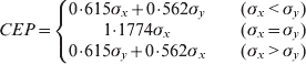
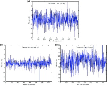
The respective error distributions in X, Y and Z coordinates from 750 simulation experiments are shown in Figure 8, where the horizontal axis represents the n-th simulation experiment, and the vertical axis represents the error (unit: m). From Figure 8, the majority of translational errors in X, Y and Z coordinates are in the interval [−3m, 3m], [−5m, 5m] and [−20m, 20m] respectively. The width of each pixel in the image at the height of 2000m represents the size of 2·2559m in actual ground width. The majority of translational errors in X and Y coordinates are within two pixels while they are under 1% in Z coordinate. CEP is 3·9872m according to equation (14). The same result can also be obtained from Table 2.

Figure 8.

The respective errors in X, Y and Z coordinates from 750 times experiments.

Table 2.

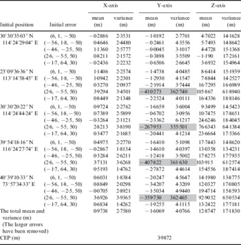
The mean and variance of errors in the X-axis, Y-axis and Z-axis from 750 times experiments.

The mean and variance of errors in the X-axis, Y-axis and Z-axis from 750 times experiments are shown in Table 2. The error unit in X and Y coordinates is pixel and the error unit in Z coordinate is metre. There exist large error points (marked data) though most of the errors in X, Y and Z coordinates are small from Table 2. Those marked datas have been removed in calculating the total mean and variance of error.

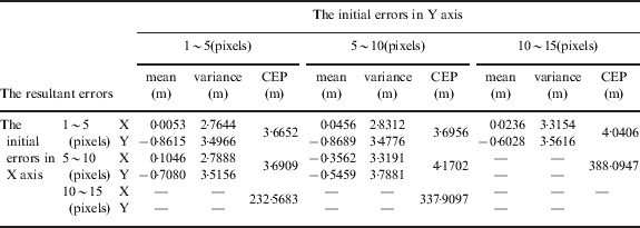
CEP is an intuitive measure of testing the accuracy of the missile system. Different initial errors may result in different CEPs, and some initial errors may produce large CEP which do not satisfy the accuracy requirements of the navigation system. In order to study the range of initial error, many experiments were done. There were nine groups of experiments and each group was repeated 750 times. The initial error in Z coordinate is always in the interval [−50m, 50m]. The initial errors in X, Y and Z coordinates are chosen randomly. The experimental results are shown in Table 3. From Table 3, we can see that if the initial errors in both X and Y coordinates are under 10 pixels, the CEP will be less than 4·2m, which can meet the accuracy requirement. If the initial error in X coordinate or in Y coordinate is larger than 10 pixels, the CEP will become very large, and it cannot be calculated.

Table 3.

The mean and variance of errors under different initial errors in X and Y coordinates.

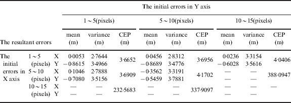
Note: “—” denotes the value can not be computed.