2.1 The resonance wave tank

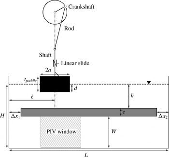
To investigate the behaviour of a valveless pump with a free surface, consider the configuration sketched in figure 1. The resonance wave tank is a simple rectangular tank with a rectangular submerged plate spanning all the tank width (out-of-plane direction in figure 1) and almost its entire length. The tank length is $L=77.4\pm 0.1~\text{cm}$ and its width is $l=25\pm 0.1~\text{cm}$ (out-of-plane direction in figure 1). The total water depth is $H=10.82\pm 0.1~\text{cm}$ . The tank is made of Plexiglas plates.

Figure 1.

Sketch of the resonance wave pump at rest, showing the tank of length $L$ , the submerged plate (shaded in grey) of thickness $e$ , the paddle at its mean position (shaded in black), the motion controller and the position of the undisturbed water surface (dashed line). Important parameters are: the main depth for wave propagation ( $h$ ), the length of the openings ( $\unicode[STIX]{x0394}x_{i}$ ), the paddle length ( $2a$ ), the paddle mean draft ( $d$ ), the paddle location ( $\ell$ ) and the height of water under the submerged plate ( $W$ ).

The submerged plate is fixed at a water depth of $h=3.5\pm 0.05~\text{cm}$ below the undisturbed free surface. The lengths of the openings on each side are identical: $\unicode[STIX]{x0394}x_{\{1,2\}}=2.9\pm 0.05~\text{cm}$ . The water can recirculate under the plate in a rectangular section of height $W=6.19\pm 0.05~\text{cm}$ through those openings.

The submerged Plexiglas plate has semicircular grooves cut out on the sides pressed against the tank walls. Rubber tubings fill the grooves and ensure a tight seal between the tank and the plate. To further ensure no leaks near the tank walls, waterproof tape was carefully added on the sides. Small rectangular holders fixed to the wall of the tank are used to support the plate. Their obstructions (less than 1.2 cm in width) are small when compared to the tank width, and thus their effects on the flow are negligible.

Table 1.

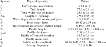
Experimental parameter ranges.

To pinch the water surface, a rectangular paddle of variable length $2a$ , thickness $t_{paddle}$ and spanning almost the total width of the tank (out-of-plane direction) is positioned at an off-centred position. Its mean draft is at a depth of $d=0.7\pm 0.05~\text{cm}$ (see table 1). The distance between the left wall of the tank and the centre of the paddle is denoted $\ell$ . The paddle is attached to three shafts at its centreline. The shafts are blocked in translation and the central one is attached to a stepper motor with a crankshaft and rod (see figure 1). This system transforms the rotational motion of the stepper motor into reciprocating translation. The rod is approximately 10 times longer than the crankshaft. The length of the crankshaft directly controls the amplitude of the paddle motion. If the motor rotates at a constant rotational velocity, the transformed motion is a quasi-sinusoidal translation. The deviation of the paddle from its mean position is denoted $S(t)$ . The amplitude ( $S_{0}$ ) and forcing frequency ( $f_{0}$ ) of the stroke are varied in this paper. The stroke motion is quasi-sinusoidal ( $S(t)\approx S_{0}\cos (2\unicode[STIX]{x03C0}f_{0}t)$ ). The values are listed in table 1. In the free-surface part of the tank (above the submerged plate), the expected wave speed, from linear water wave theory, is

(2.1) $$\begin{eqnarray}c=\frac{\unicode[STIX]{x1D714}}{k(\unicode[STIX]{x1D714})},\end{eqnarray}$$

where $\unicode[STIX]{x1D714}=2\unicode[STIX]{x03C0}f_{0}$ is the angular frequency and $k$ is the wavenumber verifying the dispersion relation

(2.2) $$\begin{eqnarray}\unicode[STIX]{x1D714}^{2}=gk\tanh (kh).\end{eqnarray}$$

Solving for the frequency range of the experiment, the wave speed is between 0.54 and $0.59~\text{m}~\text{s}^{-1}$ . A wave travels through the entire tank in approximately 1.4 s (or a frequency of 0.7 Hz). The frequency range thus encompasses the natural resonance frequencies of the tank. The lower band of 0.3 Hz is chosen to avoid seeing parasitic stepper motor motion and also to have a large enough flow to be measured. The upper band is bounded by three-dimensional effects (lateral sloshing). The width of the tank $l$ gives the expected first symmetric transverse resonance frequency

(2.3) $$\begin{eqnarray}f_{1}=\sqrt{\frac{g}{2\unicode[STIX]{x03C0}l}\tanh \frac{2\unicode[STIX]{x03C0}h}{l}}\approx 2\,\text{Hz}\end{eqnarray}$$

above the submerged plate.

In the results presented in this paper, the paddle length $2a$ , the forcing frequency $f_{0}$ and the stroke amplitude $S_{0}$ are varied. The tank length $L$ is fixed by design. The other parameters are selected consistently with previous experiments for a Liebau pump with flexible tubings. The position of the paddle is chosen such that $\ell /L\approx 25$  %, similarly to previous results for Liebau-type pumps with a flexible membrane (Rinderknecht et al. Reference Rinderknecht, Hickerson and Gharib2005; Avrahami & Gharib Reference Avrahami and Gharib2008; Meier Reference Meier2011) and is kept constant throughout this study. The water depth above the submerged plate $h$ is selected in comparison with the radius of the flexible tubes. In previous reference studies by Rinderknecht et al. (Reference Rinderknecht, Hickerson and Gharib2005) and Avrahami & Gharib (Reference Avrahami and Gharib2008), a typical ratio of inner radius to flexible tube length is of the order of 0.05. The free surface plays the role of the flexible membrane and thus the elastic forces are replaced by gravitational and surface tension forces. With the present water depth and range of frequencies, the Bond number, which compares the gravity and the surface tension forces, is

(2.4) $$\begin{eqnarray}Bo=\frac{\unicode[STIX]{x1D70C}g}{\unicode[STIX]{x1D70E}k^{2}}\approx 300{-}3000,\end{eqnarray}$$

where $\unicode[STIX]{x1D70E}\approx 0.074~\text{N}~\text{m}^{-1}$ is the surface tension and $\unicode[STIX]{x1D70C}\approx 1000~\text{kg}~\text{m}^{-3}$ is the density of water. The surface tension is thus negligible in the present study. The elastic storage of energy of the original Liebau-type pump is replaced by potential storage of energy. The total water depth $H$ and the recirculation height $W$ are linked through the submerged plate thickness $e$ . The value of $H$ is empirically chosen to have a noticeable water depth jump between the shallow part (of depth $h$ ) and the deep part (of depth $H$ ). With the present value, the ratio of wave speed between these two different water depth regions is of the order of $1/2$ . The recirculation height $W$ appeared to be suitable for the measurement method used and is presented in the next section. Another fixed parameter in the present study is the length of the openings $\unicode[STIX]{x0394}x_{i}$ . This is another unique characteristic of the free-surface version of the Liebau pump. In the original version the connection between the flexible tube and the rigid tube is made through a no-surface-displacement boundary condition. This is not possible for the free-surface pump. The selected value was arbitrarily chosen to be small when compared to the wavelength, $\unicode[STIX]{x1D706}=2\unicode[STIX]{x03C0}/k$ , of the surface waves such that a full wave could not fit above the openings (here $\unicode[STIX]{x0394}x_{i}/\unicode[STIX]{x1D706}\approx 0.02{-}0.1$ ). The limit $\unicode[STIX]{x0394}x_{i}/\unicode[STIX]{x1D706}\rightarrow \infty$ is close to the study of waves above a submerged plate in the open ocean (Graw Reference Graw1992, Reference Graw1993; Touboul & Rey Reference Touboul and Rey2012). The mean draft of the paddle is chosen such that the paddle is at the free surface in its upper position for the stroke amplitude $S_{0}=0.69~\text{cm}$ . Its thickness is selected such that the paddle is not completely immersed for the largest amplitude $S_{0}=1.16~\text{cm}$ and the largest paddle $2a=19.87~\text{cm}$ , in the absence of waves.

2.2 Data acquisition

Two cameras are used to capture the data. A first camera (Imperex IPX-2M30-L with a Vivitar 28–85 mm lens) is used to record the PIV window with a frame rate of 60 frames per second (fps) and an exposure time of 3 ms (see figure 1). The image resolution is $680\times 325$ pixels. The water is seeded with silver-coated hollow ceramic spheres of typical diameter $100~\unicode[STIX]{x03BC}\text{m}$ and specific averaged density of 1.10 g cm $^{-3}$ (Conduct-O-Fil AG-SL150-30-TRD). To keep only buoyant particles, the water used to fill the tank was prepared with particles 24 hours prior to the experiment in separate buckets. Only water away from the surface and the bottom of the buckets was used to fill the tank. To illuminate the particles, a continuous 1 W 532 nm green laser (Wicked Laser) and cylindrical lens are used to create a laser sheet. To avoid light pollution, a green filter was aligned with the camera. The PIV data are analysed using the open-source code MATLAB PIVlab (Thielicke & Stamhuis Reference Thielicke and Stamhuis2014a ,Reference Thielicke and Stamhuis b ). The code enables subpixel accuracy.

A second camera (Nikon 1 S1 with lens 1 Nikkor 11–27.5 mm f/3.5–5.6) is used to record the entire resonance wave tank. The laser illuminates the surface. For certain cases, in addition to the laser, a white projector was used with a red filter to illuminate the paddle. The green filter on the PIV camera limits the pollution induced on the PIV. The motion of the paddle was recorded. The frame rate of this camera is also set to 60 fps. The two cameras are synchronised in the case where the motion of the paddle is tracked using an additional light source. Because of the long tank and small wave height, this information is used not for quantitative measurement but for a qualitative visualisation of wave dynamics generated by the paddle.

3.1 Bulk and oscillatory flow rate and transient response

In this section, a paddle of length $2a=10.46~\text{cm}$ is considered. The paddle stroke amplitude is fixed to $S_{0}=0.69~\text{cm}$ . Different forcing frequencies are used and are referred to in the following figures.

Figure 2.

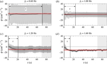
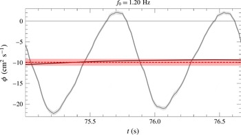
Transient response of the integrated PIV flow rate under the submerged plate for different frequencies with a paddle of length $2a=10.46~\text{cm}$ and a fixed stroke amplitude of $S_{0}=0.69~\text{cm}$ . The black solid line is a filtered curve of the instantaneous flow rate (in grey) obtained using the moving average formula of (3.1). The red dashed horizontal line gives the asymptotic bulk flow calculated as the mean of the instantaneous one over the last 20 s (shaded window between 70 and 90 s). The shading around this horizontal line shows the uncertainties. The arrow indicates the rise time after the start of the paddle. The vertical dotted line shows the start and rise times. The asymptotic bulk flow rates are $3.64\pm 0.69$ , $1.21\pm 0.45$ , $-9.93\pm 0.77$ and $-12.05\pm 1.08~\text{cm}^{2}~\text{s}^{-1}$ for $f_{0}=0.60$ , 1.00, 1.20 and 1.60 Hz, respectively.

Flow rates per unit width (hereafter called flow rate) $\unicode[STIX]{x1D719}$ are measured by integrating the instantaneous horizontal velocity profiles of the PIV data and averaging over the entire acquisition window. The integration is made using a trapezoidal rule. The estimation of uncertainties is detailed in appendix B. Data points are missing near the wall, so the flow rate is corrected by the ratio of the actual cross-section to the visible one (referred to as cross-product correction). The flow rate is considered positive if the flow is going from left to right under the submerged plate. Typical transient responses of the flow rate are shown in figure 2 for various frequencies. The pump starts while the tank is at rest and there is a transitional stage in which the flow builds up before the instantaneous bulk flow reaches its steady state (black solid line), hereafter referred to as asymptotic regime. The instantaneous bulk flow is defined as

(3.1) $$\begin{eqnarray}\langle \unicode[STIX]{x1D719}\rangle (t)=\frac{1}{2T}\int _{t-T}^{t+T}\unicode[STIX]{x1D719}(t)\,\text{d}t,\end{eqnarray}$$

and is evaluated every 10 time steps. Two wave periods are used in the smoothing averaged calculation. No noticeable variations are observed when varying the number of periods from one to four. The integral in (3.1) is approximated using the trapezoidal rule. The time to reach a steady periodic state depends on the frequency and the stroke amplitude. The rise time, $\unicode[STIX]{x1D70F}$ , is defined as the time required to reach $98\,\%$ of the asymptotic bulk flow rate, $\overline{\langle \unicode[STIX]{x1D719}\rangle }$ , defined as the mean of the instantaneous bulk flow rate over the last 20 s of data acquisition (shaded zone in figure 2). Some fluctuations are visible and are accounted for in the uncertainty estimation (see appendix B). The choice of 20 s was made to evaluate the asymptotic characteristics (bulk and first harmonic defined later) of the flow rate on at least six wave periods. From experimental observations, one needs to wait approximately 20 wave periods to reach the steady periodic state and the steady state is reached faster when the asymptotic bulk flow is stronger. Four typical behaviours are shown in figure 2. At a frequency $f_{0}=0.60~\text{Hz}$ the pump behaves like an oscillator; the oscillations are large and a bulk flow in the positive direction eventually builds up but stays small compared to the amplitude of the oscillations. At a frequency $f_{0}=1.00~\text{Hz}$ the oscillations are smaller. A weak bulk flow rate in the positive direction can be identified. For $f_{0}=1.20~\text{Hz}$ , the pump has an interesting behaviour similar to that of efficient frequencies of a Liebau impedance pump. The flow rate reaches an asymptotic pulse flow regime after 20 s. In this regime, the flow rate oscillates between zero and a negative value, with a significant bulk component of approximately $-10~\text{cm}^{2}~\text{s}^{-1}$ . At a frequency $f_{0}=1.60~\text{Hz}$ the flow becomes unidirectional with small oscillations compared to the bulk component: it is rectified. These typical flow rate behaviours are similar to that reported in previous studies of impedance pumps of Liebau type with flexible membranes.

Figure 3.

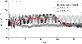
Transient response for varied forcing frequency. The black curve shows the disturbed case, the grey curves the undisturbed cases with constant forcing frequency. The red curve is the filtered curve of the instantaneous flow rate of the disturbed experiment. For the disturbed case, the tank is first randomly agitated, then the paddle is forced to oscillate at a frequency $f_{0}=1.00~\text{Hz}$ . After a minute the frequency of the paddle is switched to $f_{0}=1.60~\text{Hz}$ .

To verify the influence of the initial conditions, a test was done starting with a disturbed tank, then switching the paddle forcing frequency from a frequency for which the observed bulk flow is positive ( $f_{0}=1.00~\text{Hz}$ ) to a forcing frequency for which the observed bulk flow $\langle \unicode[STIX]{x1D719}\rangle$ is negative ( $f_{0}=1.60~\text{Hz}$ ) when starting from a tank at rest. The result of this trial is shown in figure 3. The flow rate quickly converges to the undisturbed forcing frequency cases irrespective of the initial perturbation. This shows that the regimes observed are asymptotic and independent of the initial conditions.

Figure 4.

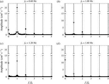
Frequency response for a given forcing frequency for a paddle of length $2a=10.46~\text{cm}$ and a fixed stroke amplitude of $S_{0}=0.69~\text{cm}$ . The results are obtained by performing a fast Fourier transform of the flow rate on 13, 23, 30 and 45 wave periods for the different frequencies $f_{0}$ (0.60, 1.00, 1.20 and 1.60 Hz, respectively). The dashed line shows for each forcing frequency the different harmonics $nf_{0}$ where $n=0,1,2,\ldots .$

Figure 5.

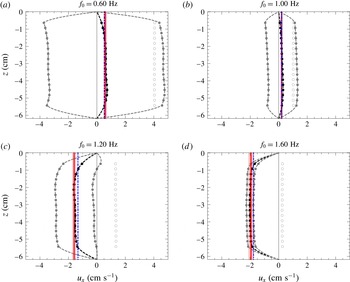
Time-averaged velocity and standard deviation from the mean profiles during a period for a paddle of length $2a=10.46~\text{cm}$ and a fixed stroke amplitude of $S_{0}=0.69~\text{cm}$ . The black filled circles are obtained by averaging the PIV data on 13, 23, 30 and 45 wave periods for the different frequencies (0.60, 1.00, 1.20 and 1.60 Hz, respectively). The grey filled circles show the averaged velocity plus/minus the standard deviation on this time sample. The empty circles show the standard deviation alone and are independent of the $z$ coordinate. The dashed lines are interpolation of the data with no-slip conditions at the wall. The red solid line shows the mean steady-state velocity calculated using the cross-product correction. The shaded zone shows the uncertainty. The blue dot-dashed line is the mean time-averaged velocity calculated after integration of the time-averaged profile interpolation.

To see the frequency signature of the flow, fast Fourier transform (FFT) analysis is applied to the data samples of 13, 23, 30 and 45 wave periods for the different frequencies (0.60, 1.00, 1.20 and 1.60 Hz, respectively). The sample size is increased with the forcing frequencies to diminish the effect of the low-frequency oscillations observed when the steady periodic state is reached. The results are shown in figure 4. The data are displayed to show the amplitude of the frequency response in absolute value. A distinctive peak is visible at each forcing frequency harmonic $nf_{0}$ where $n=0,1,2,\ldots$ . In addition, the asymptotic bulk flow rate $\overline{\langle \unicode[STIX]{x1D719}\rangle }$ defined previously is displayed with its uncertainties in grey circles.

Identically, the asymptotic first harmonic flow rate $\overline{\unicode[STIX]{x1D719}_{1}}$ is evaluated using the instantaneous first harmonic flow rate defined as

(3.2) $$\begin{eqnarray}\unicode[STIX]{x1D719}_{1}(t)=\frac{1}{T}\left|\int _{t-T}^{t+T}\text{e}^{\text{i}\unicode[STIX]{x1D714}t}\unicode[STIX]{x1D719}(t)\,\text{d}t\right|,\end{eqnarray}$$

where a factor of 2 is added to take into account the complex conjugate contribution. For the remainder of the paper, the results displaying the asymptotic bulk and first harmonic flow rate will use these integral definitions averaged over the last 20 s. The error bars estimate the uncertainties, which are mainly due to the oscillations of the instantaneous flow rate.

It is assumed that the asymptotic flow rate can be decomposed such that

(3.3) $$\begin{eqnarray}\unicode[STIX]{x1D719}(t)\approx \overline{\langle \unicode[STIX]{x1D719}\rangle }+\overline{\unicode[STIX]{x1D719}_{1}}\cos (\unicode[STIX]{x1D714}_{0}t+\unicode[STIX]{x1D703}_{1})+\overline{\unicode[STIX]{x1D719}_{2}}\cos (2\unicode[STIX]{x1D714}_{0}t+\unicode[STIX]{x1D703}_{2})+\cdots \,.\end{eqnarray}$$

For each selected frequency, figure 5 shows the velocity profile under the submerged plate at the steady periodic state and the standard deviation. The profiles are obtained by averaging over 13, 23, 30 and 45 wave periods for the different frequencies (0.60, 1.00, 1.20 and 1.60 Hz, respectively) and taking the standard deviation. The standard deviation (empty circles in the figures) appears to be constant over the entire cross-section of the recirculation section. In other words, the oscillations are nearly uniform on the entire cross-section. Slip boundary conditions are thus acceptable for the instantaneous flow rate and to describe the oscillatory part of the flow. Figure 5 also shows the mean steady periodic state velocity calculated using the cross-product correction (red solid line) and averaging on the last 20 s,

(3.4) $$\begin{eqnarray}U_{mean}=\frac{1}{W}\left\langle \frac{W}{w_{PIV}}\int _{w_{PIV}}u_{x}(y,t)\,\text{d}y\right\rangle _{T_{0}}=\frac{\overline{\langle \unicode[STIX]{x1D719}\rangle }}{W},\end{eqnarray}$$

or integrated on the cross-section after interpolation forcing the flow to be zero at the walls (see the black dashed line outlining the velocity profile and the blue dot-dashed line),

(3.5) $$\begin{eqnarray}U_{mean}=\frac{1}{W}\int _{W}\langle u_{x}(y,t)\rangle _{T_{0}}\,\text{d}y,\end{eqnarray}$$

where $\langle \,\cdot \,\rangle _{T_{0}}$ denotes the time average and $w_{PIV}$ the width of the PIV window. For the sake of simplicity, the asymptotic values are calculated using the cross-product correction for the remainder of the paper.

Figure 6.

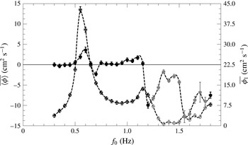
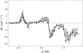
Bulk and first harmonic flow rate as a function of the forcing frequency (filled and empty circles and left and right axis, respectively) for a paddle of length $2a=10.46~\text{cm}$ and a fixed stroke amplitude of $S_{0}=0.69~\text{cm}$ . The points shaded in grey indicate cases where the bulk flow is larger than the amplitude of the oscillatory first harmonic flow rate. The scales are not the same on the two vertical axes.

3.2 Forcing frequency effect on the asymptotic bulk and oscillatory flow responses

In this section, the effect of varying the forcing frequency is examined for the asymptotic bulk and first harmonic flow rate. A series of experiments using a paddle of length $2a=10.46~\text{cm}$ and a fixed stroke amplitude of $S_{0}=0.69~\text{cm}$ are performed over a forcing frequency range 0.30–1.80 Hz with stepping of 0.05 Hz. The results are shown in figure 6. It is observed that the bulk and harmonic flow vary significantly with the forcing frequency. The bulk flow seems to be stronger near abrupt changes in the first harmonic, near resonance. These results are quite similar to the observations made in previous works done with micro-scale impedance pumps (Hickerson & Gharib Reference Hickerson and Gharib2006; Avrahami & Gharib Reference Avrahami and Gharib2008; Meier Reference Meier2011). It is interesting that, even with a drastically different scale and the absence of compliant tubes, the resonance mechanism still provides a pumping action.

In the next section, the free-surface dynamics is described for different characteristic frequencies along the spectrum.

3.3 Bulk flow rate and surface characteristics

Figure 7.

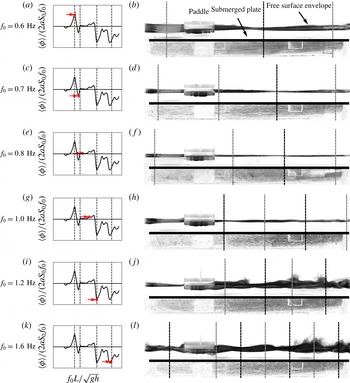
Surface envelope for different frequencies. Six characteristic free-surface envelopes are shown. The graph on (a,c,e,g,i,k) gives the non-dimensional bulk flow rates with the positions of the resonance frequencies found by solving the linearised potential problem of § 3.4. The frequency point of each row is underlined in red with an arrow pointing at it. A negative value of the bulk flow rate means that the particles are moving to the left under the submerged plate. On (b,d,f,h,j,l) the picture is obtained by taking the standard deviation of five wave periods sampled at 60 fps. The result is the envelope of the surface elevation. Under the submerged plate, PIV particles are visible and some streamlines can be observed. The grey (black) dashed lines give the position of the antinodes (nodes) found by solving the linearised problem. The paddle length and the stroke amplitude are fixed to $2a=10.46~\text{cm}$ and $S_{0}=0.69~\text{cm}$ , respectively.

In this section, the paddle length and the stroke amplitude are fixed to $2a=10.46~\text{cm}$ and $S_{0}=0.69~\text{cm}$ , respectively. Six representative forcing frequencies are considered ( $f_{0}=\{0.60,0.70,0.80,1.00,1.20,1.60\}~\text{Hz}$ ). Videos of the free-surface dynamics can give insights into the pumping mechanism. Figure 7 shows free-surface envelopes and non-dimensional bulk flow rates (described in the next section). In all formed envelopes, characteristic wave features (nodes and antinodes for the surface displacement) are observed. The dashed lines on the figure give the positions of these special points deduced by solving the linear problem described in the next section.

For $f_{0}=0.60~\text{Hz}$ , the amplitude of the waves on the left of the paddle is larger than that of those on the right. This suggests lower steady pressure points on the left side of the paddle than on the right, and consequently one can expect a suction from the right side of the paddle (downstream) towards the left (upstream) in agreement with the observed mean flow for this case. The flow is upstream above the submerged plate and thus one can expect the wave features (nodes and antinodes) to be shifted in this direction.

For $f_{0}$ between 0.70 and 1.00 Hz, the surface is rather calm. The amplitudes are noticeably larger on the left side of the paddle for $f_{0}=1.00~\text{Hz}$ . For $f_{0}=0.70~\text{Hz}$ , the surface amplitudes on both sides are close. For this case, almost half a wavelength fits on the left side. Thus we are close to the first wave resonance on this side.

For $f_{0}=1.20$ and 1.60 Hz, the surface reveals high-amplitude breaking and travelling waves on the right side of the paddle and 1 and 1.5 wavelength fits in the right section, respectively. For $f_{0}=1.20~\text{Hz}$ , the first breaking wave feature appears between the position of the first antinode and node. The wave breaks towards the right, suggesting a drift in this direction. For $f_{0}=1.20$ and 1.60 Hz, there are two other wave breaking points near the right-hand wall aligned with a predicted antinode and node. The latter can be interpreted as a second-order response. Strong nonlinear effects are expected for these cases. The fact that there are these high agitation points on this side suggests that the steady pressure should be lower near the right wall. One can thus expect suction towards this region. Gravity limits suction from under the paddle, and thus the suction should be from the left side of the paddle to the right (i.e negative under the submerged plate), as observed.

The surface envelope outlines two different pumping mechanisms here. The first one, observed at low frequency, is dominated by the generation of a mean pressure gradient due to the larger surface oscillations on the shorter side of the paddle. The second, observed near the higher-frequency resonances, is dominated by complex wave dynamics on the longer side. The envelope outlines travelling and breaking wave characteristics. Note also that for the cases where the bulk flow is negative ( $f_{0}=0.70$ , 1.20 and 1.60 Hz), the surface envelope shows close to entire numbers of waves fitting in the right side.

In previous studies with tubes, the resonance frequencies were roughly estimated by evaluating the tube wave speed and dividing by twice the tube length (Hickerson & Gharib Reference Hickerson and Gharib2006). As Meier (Reference Meier2011) pointed out, this does not take into account the mass of the fluid in the recirculation section. In the case of the tube pump, it is rather complex to evaluate the actual resonance frequencies analytically due to the complex fluid–structure interactions. In previous works (Avrahami & Gharib Reference Avrahami and Gharib2008; Meier Reference Meier2011), a step impulse was applied to the system to determine the resonance frequencies experimentally or numerically. In the resonance wave pump case, using the potential Stokes linear theory, it is possible to evaluate the first-order frequency response and deduce the resonance frequencies. In the next section, a potential theory approach is described and a model is proposed to qualitatively characterise the pump dynamics.

3.4 Potential theory

The configuration considered here, if inspired by Liebau pumps with flexible tubings, is quite similar to classical water wave problems but in a closed tank. A water wave problem approach is used to describe the asymptotic regime reached in the experiments. The wave breaking phenomenon is ignored for now. The eigenfunction expansion matching method is used to evaluate the first-order solution. Details on the mathematical technique can be found in textbooks, such as Linton & McIver (Reference Linton and McIver2001). This method was previously applied to a variety of configurations involving waves and submerged/floating obstacles (radiation of a wave by a buoy and wave above a submerged plate (Takano Reference Takano1960; Mei & Black Reference Mei and Black1969; Lee Reference Lee1995; Zheng, You & Shen Reference Zheng, You and Shen2004; Touboul & Rey Reference Touboul and Rey2012)).

Classically, for water wave problems, the potential theory is used. In this approach, solutions of the problem satisfy the Laplace equation:

(3.6) $$\begin{eqnarray}\unicode[STIX]{x0394}\widetilde{\unicode[STIX]{x1D711}}(x,z,t)=0,\end{eqnarray}$$

where $\widetilde{\unicode[STIX]{x1D711}}$ is the scalar velocity potential and $\widetilde{\boldsymbol{u}}=\unicode[STIX]{x1D735}\widetilde{\unicode[STIX]{x1D711}}$ . The fully nonlinear equations corresponding to the free-surface kinematic and dynamic boundary conditions are given by

(3.7) $$\begin{eqnarray}\displaystyle \frac{\unicode[STIX]{x2202}\widetilde{\unicode[STIX]{x1D702}}}{\unicode[STIX]{x2202}t}+\displaystyle \frac{\unicode[STIX]{x2202}\widetilde{\unicode[STIX]{x1D711}}}{\unicode[STIX]{x2202}x}\displaystyle \frac{\unicode[STIX]{x2202}\widetilde{\unicode[STIX]{x1D702}}}{\unicode[STIX]{x2202}x}=\displaystyle \frac{\unicode[STIX]{x2202}\widetilde{\unicode[STIX]{x1D711}}}{\unicode[STIX]{x2202}z}\quad \text{on }z=\widetilde{\unicode[STIX]{x1D702}},\end{eqnarray}$$

(3.8) $$\begin{eqnarray}\displaystyle \frac{\unicode[STIX]{x2202}\widetilde{\unicode[STIX]{x1D711}}}{\unicode[STIX]{x2202}t}+\frac{\widetilde{u}^{2}}{2}+g\widetilde{\unicode[STIX]{x1D702}}=0\quad \text{on }z=\widetilde{\unicode[STIX]{x1D702}},\end{eqnarray}$$

where $\widetilde{\unicode[STIX]{x1D702}}$ denotes the free-surface displacement and $g$ is the gravitational acceleration. Deriving (3.8) with respect to time and using (3.7) and (3.8), a general condition for $\widetilde{\unicode[STIX]{x1D711}}$ independent of $\widetilde{\unicode[STIX]{x1D702}}$ can be written:

(3.9) $$\begin{eqnarray}\displaystyle \frac{\unicode[STIX]{x2202}^{2}\widetilde{\unicode[STIX]{x1D711}}}{\unicode[STIX]{x2202}t^{2}}+\displaystyle \frac{\unicode[STIX]{x2202}\widetilde{u}^{2}}{\unicode[STIX]{x2202}t}+g\displaystyle \frac{\unicode[STIX]{x2202}\widetilde{\unicode[STIX]{x1D711}}}{\unicode[STIX]{x2202}z}+\frac{1}{2}\widetilde{\boldsymbol{u}}\boldsymbol{\cdot }\unicode[STIX]{x1D735}\widetilde{u}^{2}=0\quad \text{on }z=\widetilde{\unicode[STIX]{x1D702}}.\end{eqnarray}$$

These boundary conditions are completed by no-through-flow conditions at the fixed boundaries,

(3.10) $$\begin{eqnarray}\displaystyle \frac{\unicode[STIX]{x2202}\widetilde{\unicode[STIX]{x1D711}}}{\unicode[STIX]{x2202}n}=0\quad \text{at the fixed boundaries},\end{eqnarray}$$

and kinematic conditions at the moving paddle,

(3.11) $$\begin{eqnarray}\displaystyle \frac{\unicode[STIX]{x2202}\widetilde{\unicode[STIX]{x1D711}}}{\unicode[STIX]{x2202}n}=S_{0}\unicode[STIX]{x1D714}\cos (\unicode[STIX]{x1D714}t)\boldsymbol{e}_{z}\boldsymbol{\cdot }\boldsymbol{n}\quad \text{at the paddle},\end{eqnarray}$$

where $\unicode[STIX]{x1D714}=2\unicode[STIX]{x03C0}f_{0}$ is the paddle angular forcing frequency.

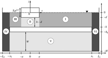
Although the important feature is the mean flow for the pump, the assumption is made here that the oscillatory part is large compared to the mean flow. This assumption might be incorrect for the flow under the submerged plate, but is more than reasonable in the upper (free-surface) part. Moreover, the problem under the submerged plate (domain V in figure 8) does not involve any nonlinear term in the potential theory. This allows the use of perturbative approach for the solutions:

(3.12) $$\begin{eqnarray}\widetilde{\unicode[STIX]{x1D711}}=\unicode[STIX]{x1D716}\widetilde{\unicode[STIX]{x1D711}}_{1}+\unicode[STIX]{x1D716}^{2}\widetilde{\unicode[STIX]{x1D711}}_{2}+O(\unicode[STIX]{x1D716}^{3}),\end{eqnarray}$$

(3.13) $$\begin{eqnarray}\widetilde{\unicode[STIX]{x1D702}}=\unicode[STIX]{x1D716}\widetilde{\unicode[STIX]{x1D702}}_{1}+\unicode[STIX]{x1D716}^{2}\widetilde{\unicode[STIX]{x1D702}}_{2}+O(\unicode[STIX]{x1D716}^{3}),\end{eqnarray}$$

where $\unicode[STIX]{x1D716}$ is a small parameter corresponding to the ratio of paddle amplitude to water depth $\unicode[STIX]{x1D716}=S_{0}/h$ . The range of $\unicode[STIX]{x1D716}$ in the experiments is from 9.6 % to 33 %. This approximation is still retained even for the largest values of $\unicode[STIX]{x1D716}$ , since it drastically simplifies the equations and enables one to evaluate the resonance frequencies, which is important in the design of such pumps.

Figure 8.

Sketch of the problem. The different shaded regions show the different domains in which the Laplace equation $\unicode[STIX]{x0394}\unicode[STIX]{x1D711}_{1}=0$ is solved with boundary conditions to generate a basis of eigenfunctions with associated eigen-numbers.

3.4.1 First-order solution: oscillatory flow

Keeping only the first-order terms, the equations can be simplified. Hereafter, complex notation is used,

(3.14) $$\begin{eqnarray}\widetilde{\unicode[STIX]{x1D711}}_{1}=\Re \{\unicode[STIX]{x1D714}S_{0}\unicode[STIX]{x1D711}_{1}(x,z)\,\text{e}^{\text{i}\unicode[STIX]{x1D714}t}\},\end{eqnarray}$$

where $\unicode[STIX]{x1D711}_{1}$ satisfies the following governing equations with boundary conditions:

(3.15) $$\begin{eqnarray}\displaystyle \frac{\unicode[STIX]{x2202}^{2}\unicode[STIX]{x1D711}_{1}}{\unicode[STIX]{x2202}x^{2}}+\displaystyle \frac{\unicode[STIX]{x2202}^{2}\unicode[STIX]{x1D711}_{1}}{\unicode[STIX]{x2202}z^{2}}=0\quad \text{(Laplace equation)},\end{eqnarray}$$

(3.16) $$\begin{eqnarray}\displaystyle \frac{\unicode[STIX]{x2202}\unicode[STIX]{x1D711}_{1}}{\unicode[STIX]{x2202}z}-\frac{\unicode[STIX]{x1D714}^{2}}{g}\unicode[STIX]{x1D711}_{1}=0,\text{ for }z=0\quad \text{and}\quad |x|\geqslant a\quad \text{(free-surface condition)},\end{eqnarray}$$

(3.17) $$\begin{eqnarray}\displaystyle \displaystyle \frac{\unicode[STIX]{x2202}\unicode[STIX]{x1D711}_{1}}{\unicode[STIX]{x2202}z} & = & \displaystyle 0,\text{ for }z=\{-h,-h_{p}\}\quad \text{and}\quad -x_{2}\leqslant x\leqslant x_{1}\nonumber\\ \displaystyle & & \displaystyle \qquad \text{(no through flow at the submerged plate)},\end{eqnarray}$$

(3.18) $$\begin{eqnarray}\displaystyle \displaystyle \frac{\unicode[STIX]{x2202}\unicode[STIX]{x1D711}_{1}}{\unicode[STIX]{x2202}x} & = & \displaystyle 0,\text{ for }-h_{p}\leqslant z\leqslant -h\quad \text{and}\quad x=\{x_{1},-x_{2}\}\nonumber\\ \displaystyle & & \displaystyle \qquad \text{(no through flow at the submerged plate)},\end{eqnarray}$$

(3.19) $$\begin{eqnarray}\displaystyle \displaystyle \frac{\unicode[STIX]{x2202}\unicode[STIX]{x1D711}_{1}}{\unicode[STIX]{x2202}z} & = & \displaystyle 0,\text{ for }z=-H\quad \text{and}\quad -L_{2}\leqslant x\leqslant L_{1}\nonumber\\ \displaystyle & & \displaystyle \qquad \text{(no through flow at the bottom of the tank)},\end{eqnarray}$$

(3.20) $$\begin{eqnarray}\displaystyle \frac{\unicode[STIX]{x2202}\unicode[STIX]{x1D711}_{1}}{\unicode[STIX]{x2202}z}=1,\text{ for }z=-d\quad \text{and}\quad |x|\leqslant a\text{ (heave condition at the paddle)},\end{eqnarray}$$

(3.21) $$\begin{eqnarray}\displaystyle \frac{\unicode[STIX]{x2202}\unicode[STIX]{x1D711}_{1}}{\unicode[STIX]{x2202}x}=0,\text{ for }z\geqslant -d\quad \text{and}\quad |x|=a\text{ (no sway at the paddle)},\end{eqnarray}$$

(3.22) $$\begin{eqnarray}\displaystyle \displaystyle \frac{\unicode[STIX]{x2202}\unicode[STIX]{x1D711}_{1}}{\unicode[STIX]{x2202}x} & = & \displaystyle 0,\text{ for }-H\leqslant z\leqslant 0\quad \text{and}\quad x=\{L_{1},-L_{2}\}\nonumber\\ \displaystyle & & \displaystyle \qquad \text{(no through flow at the side wall)},\end{eqnarray}$$

(3.23) $$\begin{eqnarray}\unicode[STIX]{x1D702}_{1}=-\frac{\text{i}\unicode[STIX]{x1D714}}{g}\unicode[STIX]{x1D711}_{1},\text{ for }z=0\quad \text{and}\quad |x|\geqslant a\text{ (free-surface displacement)},\end{eqnarray}$$

where $h_{p}=H-W$ .

In order to complete the description of the problem, the behaviour of the solution in the vicinity of the corners of the submerged plate ( $(x,z)=\{(x_{1},-h),(x_{1},-h_{p}),(-x_{2},-h),(-x_{2},-h_{p})\}$ ) and the paddle ( $(x,z)=(\pm a,-d)$ ) needs to be specified. Consider a small fluid region near one of the corners of the submerged plate or the paddle (hereafter referred to as the obstacle). Cylindrical coordinates $(r,\unicode[STIX]{x1D703})$ are introduced with origin at the considered corner such that the sides of the obstacle correspond to $\unicode[STIX]{x1D703}=0$ and $\unicode[STIX]{x1D703}=3\unicode[STIX]{x03C0}/2$ . The boundary conditions on the wall of the obstacle are $\unicode[STIX]{x2202}\unicode[STIX]{x1D711}_{1}/\unicode[STIX]{x2202}\unicode[STIX]{x1D703}=0$ on $\unicode[STIX]{x1D703}=0,3\unicode[STIX]{x03C0}/2$ . The solution must therefore satisfy $\unicode[STIX]{x1D711}_{1}\sim c+r^{2/3}\cos (2\unicode[STIX]{x1D703}/3)$ as $r\rightarrow 0$ , where $c$ is a constant. This implies that the velocity field near the corners must be governed by the relation

(3.24) $$\begin{eqnarray}\unicode[STIX]{x1D735}\unicode[STIX]{x1D711}_{1}=\boldsymbol{O}(r^{-1/3})\quad \text{as}\;r\rightarrow 0.\end{eqnarray}$$

The tank is cut into six rectangular domains (numbered from I to VI as shown in figure 8). In each domain the Laplace equation with natural boundary conditions is solved by means of separation of variables. This yields a basis of eigenfunctions with associated eigen-wavenumbers. The solution can be written as an infinite series of orthogonal functions in each domain, which satisfies all the boundary conditions with unknown coefficients to be determined. For instance, for domain I,

(3.25) $$\begin{eqnarray}\displaystyle \unicode[STIX]{x1D711}_{1}^{\text{I}} & = & \displaystyle \{A_{0}^{\text{I}}\,\text{e}^{-\text{i}k(x-x_{1})}+B_{0}^{\text{I}}\,\text{e}^{\text{i}k(x-x_{1})}\}q_{0}(z)\nonumber\\ \displaystyle & & \displaystyle +\mathop{\sum }_{n\geqslant 1}\{A_{n}^{\text{I}}\,\text{e}^{-\unicode[STIX]{x1D6FC}_{n}(x-x_{1})}+B_{n}^{\text{I}}\,\text{e}^{\unicode[STIX]{x1D6FC}_{n}(x-x_{1})}\}q_{n}(z),\end{eqnarray}$$

where $A_{j}^{i}$ and $B_{j}^{i}$ are unknown coefficients, $k$ and $\unicode[STIX]{x1D6FC}_{n\geqslant 1}$ are eigenvalues in domains I and III, and $q_{n\geqslant 0}$ are the eigenfunctions given by

(3.26) $$\begin{eqnarray}\displaystyle & \displaystyle q_{0}(z)=\cosh [k(h+z)]\quad \text{ where }k\tanh (kh)=\unicode[STIX]{x1D714}^{2}/g, & \displaystyle\end{eqnarray}$$

(3.27) $$\begin{eqnarray}\displaystyle & \displaystyle q_{n}(z)=\cos [\unicode[STIX]{x1D6FC}_{n}(h+z)]\quad \text{ where }\unicode[STIX]{x1D6FC}_{n}\tan (\unicode[STIX]{x1D6FC}_{n}h)=-\unicode[STIX]{x1D714}^{2}/g. & \displaystyle\end{eqnarray}$$

The eigenvalues are evaluated numerically using a Newton–Raphson method. For the initial guess values, approximations given by Chamberlain & Porter (Reference Chamberlain and Porter1999) are used.

The coefficients are found numerically by forcing the continuity of $\unicode[STIX]{x1D711}_{1}$ and its normal derivative and truncating the expansions to a finite number of terms. For the sake of brevity, all the equations are reported in appendix A. The edge conditions of the form of (3.24) give the behaviour of the coefficients for large $n$ . Using Mellin transforms (Martin Reference Martin1995), it is possible to show that

(3.28) $$\begin{eqnarray}\mathop{\sum }_{n=1}^{\infty }n^{-2/3}\text{e}^{-nx}\sim \unicode[STIX]{x1D6E4}(1/3)x^{-1/3}\quad \text{as}\;x\rightarrow 0^{+},\end{eqnarray}$$

and it follows that

(3.29a,b ) $$\begin{eqnarray}A_{n}^{\text{I}}\,\text{e}^{\unicode[STIX]{x1D6FC}_{n}\left(x_{1}-a\right)}=O(n^{-5/3}),\quad B_{n}^{\text{I}}=O(n^{-5/3})\quad \text{as}\;n\rightarrow \infty .\end{eqnarray}$$

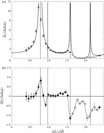
The results shown here are found using a 10-term expansion in each domain. This number of terms was found to be sufficient in the present applications, as computations with a larger number of terms did not exhibit any significant difference in the results. It is then possible to evaluate the first harmonic flow rate, $\overline{\unicode[STIX]{x1D719}_{1}}$ under the submerged plate. For comparison with the experiments, the flow rate is non-dimensionalised by half the rate of volume displaced by the paddle (volume times the frequency) as suggested by Thomann (Reference Thomann1978) and Hickerson & Gharib (Reference Hickerson and Gharib2006) and done in Avrahami’s computational work (Avrahami & Gharib Reference Avrahami and Gharib2008). The results are displayed in figure 9.

Figure 9.

Non-dimensional first harmonic ( $a$ ) and bulk ( $b$ ) flow rate as a function of the non-dimensional forcing frequency (empty and filled circles, respectively) for a paddle of length $2a=10.46~\text{cm}$ and a fixed stroke amplitude of $S_{0}=0.69~\text{cm}$ . The points shaded in grey indicate cases where the bulk flow is larger than the oscillatory first harmonic flow rate. The black solid line in ( $a$ ) is obtained by solving the linear problem as formulated in § 3.4. The dashed vertical lines show the position of the resonances.

Figure 9( $a$ ) shows the first harmonic response and figure 9( $b$ ) the bulk flow. The bulk flow is stronger in the vicinity of resonance frequencies. Near these frequencies, the first harmonic response found experimentally appears to be damped due to a nonlinear effect (wave breaking). Thus, as expected, the linear theory is not valid near these frequencies.

A more detailed description of the eigenfunction matching method used here is presented in appendix A. The theory is an important tool for a designing resonance wave tank since it provides good estimates of the important frequencies. It is shown in § 3.5 that it is consistent with variation of paddle size. A similar method could be applied to the flexible tube version to estimate the resonance frequencies.

However, this analysis neither gives an estimate of the bulk flow rate nor predicts the preferred directions of pumping. It is possible to expand the linear theory to the next order, which would yield a steady term depending on the first-order term.

3.4.2 Effect of the wave field on the mean flow

The wave field can act on the mean flow in two ways: an interaction stress tensor,

(3.30) $$\begin{eqnarray}\unicode[STIX]{x1D61B}_{ij}^{int}=-\langle \widetilde{u}_{i}\widetilde{u}_{j}\rangle -\unicode[STIX]{x1D6FF}_{ij}p^{w},\end{eqnarray}$$

which governs the transfer of momentum from the waves to the mean motion, where $p^{w}$ is the mean pressure due to the wave field; and a transfer of mass due to the divergence of the Stokes mass transport,

(3.31) $$\begin{eqnarray}M_{x}^{w}=\left<\int _{0}^{\widetilde{\unicode[STIX]{x1D702}}}\widetilde{u}_{x}\,\text{d}z\right>.\end{eqnarray}$$

This is elegantly presented by Hasselmann (Reference Hasselmann1971). In the approximation of linear waves, these expressions can be reduced to simple quadratic forms,

(3.32) $$\begin{eqnarray}\unicode[STIX]{x1D64F}^{int}=\left(\begin{array}{@{}cc@{}}\left<\displaystyle \frac{\unicode[STIX]{x2202}\widetilde{\unicode[STIX]{x1D711}}_{1}}{\unicode[STIX]{x2202}z}^{2}-\displaystyle \frac{\unicode[STIX]{x2202}\widetilde{\unicode[STIX]{x1D711}}_{1}}{\unicode[STIX]{x2202}x}^{2}\right> & -\left<\displaystyle \frac{\unicode[STIX]{x2202}\widetilde{\unicode[STIX]{x1D711}}_{1}}{\unicode[STIX]{x2202}z}\displaystyle \frac{\unicode[STIX]{x2202}\widetilde{\unicode[STIX]{x1D711}}_{1}}{\unicode[STIX]{x2202}x}\right>\\ -\left<\displaystyle \frac{\unicode[STIX]{x2202}\widetilde{\unicode[STIX]{x1D711}}_{1}}{\unicode[STIX]{x2202}z}\displaystyle \frac{\unicode[STIX]{x2202}\widetilde{\unicode[STIX]{x1D711}}_{1}}{\unicode[STIX]{x2202}x}\right> & 0\end{array}\right),\end{eqnarray}$$

where the wave-induced mean pressure is readily seen to be $p^{w}=-\langle \widetilde{u}_{z}^{3}\rangle$  (Hasselmann Reference Hasselmann1971), and

(3.33) $$\begin{eqnarray}M_{x}^{w}=\left<\left.\displaystyle \frac{\unicode[STIX]{x2202}\widetilde{\unicode[STIX]{x1D711}}_{1}}{\unicode[STIX]{x2202}x}\right|_{z=0}\widetilde{\unicode[STIX]{x1D702}}_{1}\right>.\end{eqnarray}$$

In the linear theory, the Stokes mass transport is equivalent to a surface current. A variation of mass in the surface layer is transmitted to the bulk of the flow (region under the mean surface position) where the linear theory is solved. It is easy to show that, in the linear theory presented in the previous subsection, $\widetilde{\unicode[STIX]{x1D711}}_{1}\propto \cos (\unicode[STIX]{x1D714}t)$ and $\widetilde{\unicode[STIX]{x1D702}}_{1}\propto \sin (\unicode[STIX]{x1D714}t)$ (from (3.23)), and thus $M_{x}^{w}$ is identically null. The only source is thus $\unicode[STIX]{x1D64F}^{int}$ . Since the general solution of the linear solution is a standing wave, the interaction stress tensor is evaluated for a scalar velocity potential $\widetilde{\unicode[STIX]{x1D711}}_{1}\propto \cosh [k(h+z)]\cos (kx)$ . It plays a role in the mean flow equations through its divergence

(3.34) $$\begin{eqnarray}\unicode[STIX]{x1D735}\boldsymbol{\cdot }\unicode[STIX]{x1D64F}^{int}\propto \frac{k^{3}}{4}\left(\begin{array}{@{}c@{}}-\sin (2kx)\cosh [2k(h+z)]\\ \cos (2kx)\sinh [2k(h+z)]\end{array}\right),\end{eqnarray}$$

and corresponds to structure of typical length $\unicode[STIX]{x1D706}/2$ . It can thus influence the mean flow for the low-frequency cases ( $f_{0}=0.6~\text{Hz}$ , $\unicode[STIX]{x1D706}/2\approx 45~\text{cm}$ ), but not significantly for the higher-frequency cases ( $f_{0}=1.2~\text{Hz}$ , $\unicode[STIX]{x1D706}/2\approx 24~\text{cm}$ and $f_{0}=1.6~\text{Hz}$ , $\unicode[STIX]{x1D706}/2\approx 17~\text{cm}$ ). The linear theory is not valid near the resonance frequencies due to wave breaking (as seen in figure 7). In the next section, dissipation is added to model the pump dynamics near the resonance.

3.4.3 Linear theory with dissipation and Stokes mass transport

From the experimental observations and the previous discussions on the wave field effect on the mean flow, it appears that dissipation is important to model the pump behaviour. In this section, a damping term is added to the linear theory to take into account the wave breaking dissipation. Consider that the surface domains have a dissipation correction such that, for instance, for domain I,

(3.35) $$\begin{eqnarray}\displaystyle \unicode[STIX]{x1D711}_{1}^{\text{I}} & = & \displaystyle \{A_{0}^{\text{I}}\,\text{e}^{-\text{i}(k-\text{i}\unicode[STIX]{x1D6FC}_{0})(x-x_{1})}+B_{0}^{\text{I}}\,\text{e}^{\text{i}(k-\text{i}\unicode[STIX]{x1D6FC}_{0})(x-x_{1})}\}q_{0}(z)\nonumber\\ \displaystyle & & \displaystyle +\mathop{\sum }_{n\geqslant 1}\{A_{n}^{\text{I}}\,\text{e}^{-\unicode[STIX]{x1D6FC}_{n}(x-x_{1})}+B_{n}^{\text{I}}\,\text{e}^{\unicode[STIX]{x1D6FC}_{n}(x-x_{1})}\}q_{n}(z),\end{eqnarray}$$

where we define

(3.36) $$\begin{eqnarray}\unicode[STIX]{x1D6FC}_{0}=k^{3}\frac{4\unicode[STIX]{x1D708}_{s}}{\unicode[STIX]{x1D714}}\frac{\sinh 2kh}{\sinh 2kh+2kh},\end{eqnarray}$$

and $\unicode[STIX]{x1D708}_{s}$ is a kinematic wave breaking viscosity. This definition is consistent with the surface dissipation due to viscosity in the limit of $\unicode[STIX]{x1D708}_{s}\rightarrow 0$ (Dutykh & Dias Reference Dutykh and Dias2007; Dias, Dyachenko & Zakharov Reference Dias, Dyachenko and Zakharov2008). Similar dissipation terms are added to the domains III, IV and VI. The dissipation correction in this simple model affects only the travelling modes. The eigenfunctions associated with these modes have to be corrected in a similar manner to verify the Laplace equation (incompressibility condition):

(3.37) $$\begin{eqnarray}q_{0}(z)=\cosh [(k-\text{i}\unicode[STIX]{x1D6FC}_{0})(h+z)].\end{eqnarray}$$

The orthogonality of this eigenfunction with the $q_{n>0}$ is not respected any more and some additional terms need to be taken into account in the projection method (see appendix A). The value of $\unicode[STIX]{x1D708}_{s}$ in the present model is selected empirically such that the wave amplitude found in the linear theory is below a threshold, $\widetilde{\unicode[STIX]{x1D702}}_{bw}$ . Miche (Reference Miche1944) gave the wave breaking criteria for water wave in the form

(3.38) $$\begin{eqnarray}\widetilde{\unicode[STIX]{x1D702}}_{bw}=\unicode[STIX]{x1D6FD}_{Miche}\frac{\tanh (k_{0}h)}{k_{0}h}h,\end{eqnarray}$$

where $\unicode[STIX]{x1D6FD}_{Miche}=0.88$ (a parameter in the present model) and $k_{0}$ is the wavenumber in the absence of dissipation. In this simple model, there are two parameters: the wave breaking threshold described by Miche’s law and the parameter $\unicode[STIX]{x1D6FD}_{Miche}$ , and the initial value of the surface viscosity $\unicode[STIX]{x1D708}_{init}$ . To solve the problem for a given forcing frequency and stroke amplitude, the following algorithm is used:

1. (1) initialise $\unicode[STIX]{x1D708}_{s}=\unicode[STIX]{x1D708}_{init}$

2. (2) while true

   1. (i) solve for $\unicode[STIX]{x1D711}_{1}^{I}$

   2. (ii) evaluate the maximum surface elevation $\widetilde{\unicode[STIX]{x1D702}}_{max}$

   3. (iii) if $\widetilde{\unicode[STIX]{x1D702}}_{max}>\widetilde{\unicode[STIX]{x1D702}}_{bw}$ , then update $\unicode[STIX]{x1D708}_{s}=\unicode[STIX]{x1D708}_{s}+\unicode[STIX]{x1D705}[\widetilde{\unicode[STIX]{x1D702}}_{max}/\widetilde{\unicode[STIX]{x1D702}}_{s}]\unicode[STIX]{x1D708}_{s}$ , else break

3. (3) end while

where $\unicode[STIX]{x1D705}$ is a parameter of the simulation for convergence (here $\unicode[STIX]{x1D705}=0.05$ ). The initial value of the wave breaking surface viscosity is arbitrarily chosen to be $\unicode[STIX]{x1D708}_{init}=4\times 10^{-4}~\text{m}^{2}~\text{s}^{-1}$ , for the numerical applications. The loop is performed with only one mode to find a suitable value of $\unicode[STIX]{x1D708}_{s}$ . A second loop is then performed with 10 modes.

Figure 10.

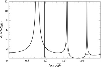
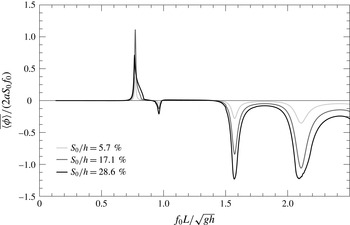
Non-dimensional first harmonic flow rate estimated with the dissipation model as a function of the non-dimensional forcing frequency (grey solid line) compared to the linear potential theory (black solid line) ( $\unicode[STIX]{x1D708}_{init}=4\times 10^{-4}~\text{m}^{2}~\text{s}^{-1}$ and $\unicode[STIX]{x1D6FD}_{Miche}=0.88$ ).

Figure 10 shows the non-dimensional first harmonic flow rate found with this model for $S_{0}/h=19.8\,\%$ (or $S_{0}=0.69~\text{cm}$ ) (grey line) compared to the potential theory (black line). Away from the resonances, the response curve of the first harmonic flow rate is not significantly modified. The first harmonic is damped in the model near the resonances, similarly to the experimental observations.

Figure 11.

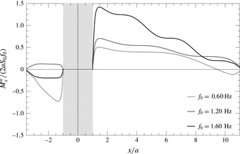
Stokes mass transport along the tank length for different frequencies for a forcing amplitude $S_{0}/h=19.8\,\%$ . The grey shaded area outlines the position of the paddle. For the frequency $f_{0}=1.20~\text{Hz}$ , the Stokes mass transport is positive in both domains.

Figure 12.

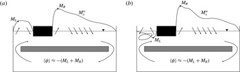
Sketches of the Stokes mass transport effect on the bulk flow for $f_{0}=1.20~\text{Hz}$ (a) and $f_{0}=1.60~\text{Hz}$ (b). The solid line shows the Stokes mass transport with a positive value if the curve is above the undisturbed free surface (dashed horizontal line). The extreme values are noted $M_{L}$ and $M_{R}$ on the left and right sides of the paddle, respectively. The bulk flow rate is estimated as the sum of the opposite of these two values.

Figure 13.

Non-dimensional bulk flow rate estimated with the dissipation model as a function of the non-dimensional forcing frequency for different forcing amplitude ( $\unicode[STIX]{x1D708}_{init}=4\times 10^{-4}~\text{m}^{2}~\text{s}^{-1}$ and $\unicode[STIX]{x1D6FD}_{Miche}=0.88$ ).

The Stokes mass transport is not identically zero any more with regard to this model. Profiles of the Stokes mass transport $M_{x}^{w}$ are shown in figure 11 for different frequencies. A positive value of $M_{x}^{w}$ means that there is a wave travelling in the positive direction. For the frequency $f_{0}=1.60~\text{Hz}$ , the Stokes mass transport is negative (positive) just after the paddle on the left (right, respectively). This can be interpreted as a general flux of mass away from the paddle. On the right side, starting from the paddle, the Stokes mass transport increases. There is a positive suction from the bulk part of the flow to the free-surface layer to build up this positive Stokes mass transport. After the position $x/a\approx 1.2$ , the Stokes mass transport starts to diminish. The wave mass is transferred back to the bulk part of the flow. A similar dynamics happens on the left side of the paddle for this frequency. This is sketched in figure 12(b). The Stokes mass transport absolute value is stronger on the right side; a flow towards the negative direction is expected under the submerged plate. A recirculation is expected on the left paddle side. For the case $f_{0}=1.20~\text{Hz}$ , the Stokes mass transport is positive in both sections of the tank. This frequency appears to be more efficient than 1.60 Hz in this simple model and as observed experimentally: there should be no recirculation on the left side (see figure 12 a). The bulk flow rate under the submerged plate is estimated as the sum of the extreme values of the Stokes mass transport on each side of the paddle. The direction of the flow under the submerged plate is in the opposite direction to this value (see figure 12).

Figure 14.

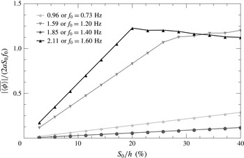
Non-dimensional bulk flow rate estimated with the dissipation model as a function of the non-dimensional stroke amplitude for different frequencies ( $\unicode[STIX]{x1D708}_{init}=4\times 10^{-4}~\text{m}^{2}~\text{s}^{-1}$ and $\unicode[STIX]{x1D6FD}_{Miche}=0.88$ ).

Figure 13 shows the non-dimensional bulk flow rate evaluated by this model as a function of the non-dimensional forcing frequency for three different forcing amplitudes. The model correctly captures the dynamics of the system. The direction of the bulk flow rate matches the experimental results near the resonances. It is observed that the directions of the peak values are not influenced by the choice of $\unicode[STIX]{x1D708}_{init}$ . The values of $\unicode[STIX]{x1D708}_{init}$ and $\unicode[STIX]{x1D6FD}_{Miche}$ have an effect on the maximum flow rate reached and the frequency ranges for which the bulk flow rate becomes significant around the resonances. The bulk flow rate varies quadratically with the forcing frequency away from the resonances. Near the resonance, the model predicts the cases of saturation due to the large values of $\unicode[STIX]{x1D708}_{s}$ required to satisfy the empirical breaking wave threshold. Figure 14 shows the non-dimensional flow rate as a function of the non-dimensional forcing stroke amplitude. For the frequency $f_{0}=1.40~\text{Hz}$ and $f_{0}=0.73~\text{Hz}$ , the non-dimensional bulk flow rate varies quadratically with the forcing. For $f_{0}=1.20~\text{Hz}$ and $f_{0}=1.60~\text{Hz}$ , a saturation is eventually reached. The non-dimensional flow rate even starts to diminish with increasing stroke amplitude in this model for $f_{0}=1.60~\text{Hz}$ . The non-dimensional stroke amplitude at which the non-dimensional flow rate starts to saturate depends on the value of $\unicode[STIX]{x1D708}_{init}$ prescribed in this model. If the value of $\unicode[STIX]{x1D708}_{init}$ is larger, the stroke amplitude of saturation is higher at a resonance.

This simple model enables one to understand the basic physics behind the free-surface resonance wave pump. It qualitatively captures the direction of the flow. To be improved, it would require one to provide a more physical way of evaluating the surface dissipation, which should not be uniform on the entire width of the tank since the wave breaking is localised in space. This is outside the scope of this paper. In the next section the stroke amplitude and the paddle size are varied experimentally.

3.5 Effect of varying the paddle stroke amplitude and length

In this section some paddle parameters are varied experimentally. First, the paddle is kept the same (length $2a=10.46~\text{cm}$ or a non-dimensionalised length of $2a/L$ = 13.5 %) and the amplitude is varied to verify the last comment of the previous section. Then to validate the linear theory to estimate the resonance frequencies, the paddle size is changed for a given stroke amplitude. Results are all non-dimensionalised.

Figure 15.

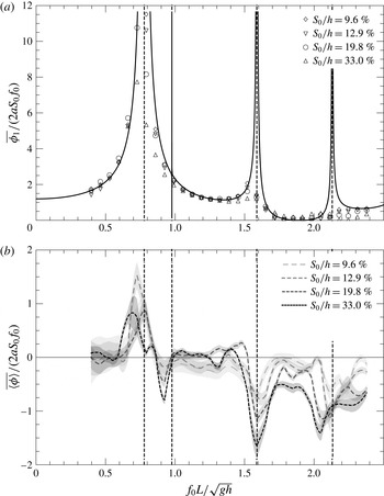
Experimental results. Non-dimensional first harmonic flow rate ( $a$ ) and bulk flow rate ( $b$ ) as a function of the non-dimensional forcing frequency for a paddle of length $2a/L=13.5\,\%$ . The stroke amplitude is varied. For the first harmonic flow, small variations are observed while varying the stroke amplitude: it is more damped near the resonance frequencies as the amplitude is increased. For the bulk flow, increasing the amplitude results in higher non-dimensional flow rates (thus efficiency) near resonance frequencies. The vertical dashed lines show the resonance frequencies found using the linear theory (values are 0.77, 1.59 and 2.13).

Figure 16.

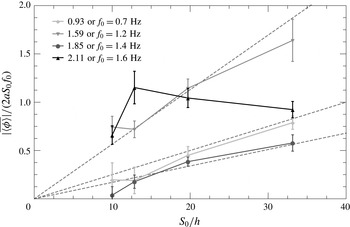
Experiment results. Absolute non-dimensional bulk flow rate as a function of the non-dimensional stroke for different forcing frequencies. For most cases, the bulk flow increases in a linear manner with the stroke amplitude. For the non-dimensional forcing frequency of 2.11, the bulk flow increases then diminishes as the stroke is increased. This can be due to a shift of apparent frequency in the tank due to the current, three-dimensional effects and competition between different pumping sources. The dashed lines show the linear trends.

Figure 15 shows the effect of varying the stroke amplitude. For the sake of clarity, the error bars and the points are removed from the non-dimensional first harmonic flow rate as a function of the non-dimensional frequency figure (figure 15 $a$ ). The linear theory correctly predict the first harmonic away from the resonances (vertical dashed lines). Near the resonance frequencies, the data fall below the linear theory, and increasing the amplitude $S_{0}/h$ leads to more damping. For instance, for the non-dimensional frequency 0.79 ( $f_{0}=0.60~\text{Hz}$ ), the linear theory predicts a resonance and experimentally the non-dimensional values are 11.55, 10.63, 8.18, 5.38 for $S_{0}/h$ values of 9.6 %, 12.9 %, 19.8 % and 33 %, respectively. Similar results are visible near the non-dimensional resonance frequencies 0.92, 1.59 and 2.11 ( $f_{0}=\{0.70,1.20,1.60\}~\text{Hz}$ ). This is consistent with the dissipation model presented in the previous section. For the bulk flow, one can see that increasing the amplitude significantly increases the non-dimensional flow rate for most forcing frequencies. For instance, the maximum non-dimensional bulk flow rate is found for $S_{0}/h=33\,\%$ at the non-dimensional frequency of 1.59 (1.20 Hz) and the value is $-1.64$ with a corresponding non-dimensional first harmonic flow rate of 1.24. The non-dimensional flow rate for $S_{0}/h=19.8\,\%$ (12.9 %, 9.6 %) is $-1.14$ ( $-0.72$ , $-0.74$ ) for the bulk flow and 1.31 (1.38, 1.43) for the first harmonic (respectively). These results are in fair agreement with the comments of the previous section and previous studies of resonance pumps with elastic tubes of Meier (Reference Meier2011). The non-dimensional first harmonic decreases (an increase in the amplitude leads to more damping near resonance frequencies) and the non-dimensional bulk flow increases with the non-dimensional forcing stroke amplitude. There is a close to quadratic dependence of the bulk flow with the forcing frequencies, consistent with the Stokes mass transport discussion. Other interesting features are also visible. For instance, at the non-dimensional frequency of 1.85 (or $f_{0}=1.40~\text{Hz}$ ), one observes nearly no flow for the lowest amplitude ( $S_{0}/h=9.6\,\%$ ) and afterwards a close to linear (quadratic) dependence of the non-dimensional (dimensional) bulk flow rate with the non-dimensional (dimensional) excitation amplitude $S_{0}/h$ ( $S_{0}$ ). This is consistent with a wave dissipation model. At the lowest amplitude, the waves are not dissipating much energy (due to breaking) and the non-dissipative theory presented here holds. Once the amplitude is increased, more wave dissipation occurs and the Stokes mass transport becomes non-zero. The bulk flow varies then close to quadratically with the excitation. On the other extreme, when the forcing frequency is near a resonance frequency, for instance the non-dimensional frequency 2.11 (or 1.60  Hz), the wave dissipation becomes so important that increasing the amplitude does not lead to a faster non-dimensional flow rate: increasing the amplitude leads to less than linear increase of the non-dimensional bulk flow rate. Figure 16 shows the influence of the stroke on the bulk flow for some selected frequencies. The close to linear dependence (see dashed lines in figure 15) for 0.93 (0.70  Hz), 1.59 (1.20 Hz) and 1.85 (1.40 Hz) of the non-dimensional mean flow with the stroke amplitude is in agreement with the linear theory induced mean flow discussion (second-order and Stokes mass transport, see figure 14) of the previous section.

Figure 17.

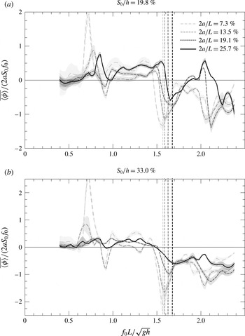
Experimental results. Non-dimensionalised bulk flow rate as a function of frequency for different paddle size and different stroke amplitude (19.8 % and 33.0 % stroke for panels ( $a$ ) and ( $b$ ), respectively). The vertical lines display the theoretical position of the second resonance where high bulk flow rates are expected (values are 1.57, 1.59, 1.63 and 1.68, respectively). Increasing the paddle size shifts the curve to the right. The observed maximum consistently diminishes with increasing paddle size.

Now, the size of the paddle is varied between 7.3 % and 25.7 % of the total length of the tank. The position of the centre of the paddle $\ell$ is kept constant. The bulk flow as a function of the frequency is displayed in figure 17 for two stroke amplitudes. Figure 17( $a$ ) and ( $b$ ) shows the results for a stroke of $S_{0}/h=19.8\,\%$ and 33.0 %, respectively. For all the cases, increasing the amplitude increases the efficiency measured here as the non-dimensional bulk flow rate. For the largest paddle, this effect is a bit diminished consistently with the previous discussion for the non-dimensional frequency 2.11 ( $f_{0}=1.60~\text{Hz}$ ). The position of the expected resonance found by the linear theory (dashed line) matches the experimental results. As one may expect, the resonance frequency increases with the paddle size. The free-surface length is reduced and higher frequencies are needed to obtain equivalent wave patterns. It is also noticeable that the smallest paddle size gives the highest non-dimensional bulk flow rate. This observation is consistent on the entire range of paddle size variation and is worth reporting. This is expected in regard to the dissipation model. For the largest paddle, the dissipation is expected to reach saturation at a lower stroke amplitude and thus a reduction of efficiency. For the smallest paddle the pumping range is limited to the vicinity of the resonance frequency predicted by the linear theory. Lastly, the maximum reported non-dimensional bulk flow rate near the outlined resonance is $-2.19$ for a paddle size $2a/L=7.3\,\%$ and stroke amplitude $S_{0}/h=33\,\%$ at a frequency of 1.59. The associated oscillatory flow rate is 1.47. This means that, for this experimental case, not only is the absolute non-dimensional bulk flow rate higher than 2 but the oscillatory part is smaller. The value of 2 is peculiar since it is the optimal value for a peristaltic pump. It is equivalent to transporting the same volume as the one displaced by the paddle at each period. One can note that there is also a peak near a non-dimensional frequency of 0.7 with a higher absolute non-dimensional bulk flow (2.75) for a paddle size $2a/L=7.3\,\%$ and stroke amplitude $S_{0}/h=33\,\%$ . This peak is associated with higher non-dimensional first harmonic flow (8.86). In this case the flow changes direction under the submerged plate over a wave period.

3.6 Energy conversion

Another interesting aspect to look at when studying pumps is the efficiency. In this case, the efficiency is defined as the quantity of input energy in the tank through the paddle per cycle transformed into net kinetic energy under the submerged plate. The energy of the oscillating part of the flow is not considered. For this application, the important part of the flow in which we are interested is the one moving the fluid in one direction. To be accurate, one should track the contact line between the paddle and the surface to evaluate the energy input. For the sake of simplicity, the energy radiated inside the fluid can be evaluated as if the paddle is in contact with the water surface at all times. This assumption results in overestimating the input energy, in general. The energy input is defined as

(3.39) $$\begin{eqnarray}\unicode[STIX]{x1D6F1}_{input}={\textstyle \frac{1}{2}}\unicode[STIX]{x1D70C}aS_{0}^{2}\unicode[STIX]{x1D714}^{2}.\end{eqnarray}$$

This energy is transformed to kinetic net flow of energy under the submerged plate:

(3.40) $$\begin{eqnarray}\unicode[STIX]{x1D6F1}_{bulk\;flow}=\frac{\unicode[STIX]{x1D70C}\overline{\langle \unicode[STIX]{x1D719}\rangle }^{2}}{2W}.\end{eqnarray}$$

The efficiency of the pump is estimated as

(3.41) $$\begin{eqnarray}\unicode[STIX]{x1D702}=\frac{\overline{\langle \unicode[STIX]{x1D719}\rangle }^{2}}{aWS_{0}^{2}\unicode[STIX]{x1D714}^{2}}.\end{eqnarray}$$

Figure 18.

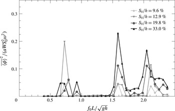
Experimental results. Non-dimensionalised energy transformation or efficiency as a function of non-dimensionalised frequency. The efficiency increases with the stroke amplitude and is highest near the resonance. The highest efficiency is 22 %.

Figure 18 shows the efficiency for the case $2a/L=13.5\,\%$ and different stroke amplitudes. It can be seen that the efficiency is higher near the resonance and that the efficiency increases with the stroke amplitude. For all the range of experiments presented in this paper, the top efficiency recorded is 22 % near the resonance. This number may seem small when compared to other water pump efficiencies. Nevertheless, the big asset of this pump is that there is no immersed mobile parts or valves. Also, in practical applications, it can be envisioned that a free source of excitation, such as wind or ocean waves, could be used to generate the waves. For instance, wind vortex shedding behind a bluff body could either excite the surface and generate the waves or control the paddle oscillations. In this case, the system should be used as a simple way of designing a pump at low cost. Positioning a turbine under the submerged plate, the device could be used as an energy converter. Then the candidate for the source of energy can also be ocean waves. One could consider having waves entering the system from the out-of-plane direction at an off-centre position (equivalent to the paddle position in the present study) or through one of the sides (extreme case of having the paddle at a wall). Having the energy converter under the submerged plate provides the opportunity to use state-of-art turbines and thus have almost no loss in the mean flow to electricity conversion and protect the converter device from extreme waves. One of the pitfalls of the system is that it appears to work for a specific range of frequencies that would need to be carefully evaluated. The potential theory gives a good estimate of the optimal frequencies. The dissipation model is intended not to predict the flow rate but to illustrate the pumping mechanism.

It is important to keep in mind that the device studied here is directly inspired by the Liebau impedance pump, which shows how nature is able to design a pump at low cost. Indeed, the Liebau pump with flexible tubings illustrates how the heart (the blood pump) works at the embryonic stage before the complex chambers and valves are developed. This is a promising system for renewable energy applications where the principal pitfalls are usually the capital cost and maintenance.