1 Introduction
Diffusion of transmembrane proteins in the plane of the plasma membrane of cells has profound biological implications because many of these proteins are involved in important signal transduction pathways which affect the cell’s function (Lodish et al. Reference Lodish, Berk, Kaiser, Scott, Bretscher, Ploegh and Matsudaira2008). Experimental studies suggest that many of these proteins exhibit complex diffusive behaviour (Tomishige, Sako & Kusumi Reference Tomishige, Sako and Kusumi1998; Weigel et al. Reference Weigel, Simon, Tamkun and Krapf2011), including anomalous diffusion (Schütz, Schindler & Schmidt Reference Schütz, Schindler and Schmidt1997). One confounding property of these systems is that rates of diffusion of molecules within the plasma membrane are one or two orders of magnitude lower than those of the same molecules reconstituted in synthetic lipid vesicles (Fujiwara et al. Reference Fujiwara, Ritchie, Murakoshi, Jacobson and Kusumi2002). Because of the wide range of intermolecular interactions within and outside the membrane that could affect diffusion, many hypotheses have been put forth for this effect. These hypotheses have, in turn, been investigated using different modelling methods. Some of these hypotheses and methods are worthy of mention here, although they are beyond the scope of this work.
Molecular dynamics simulations have provided insight into transient lipid–protein (Niemelä et al. Reference Niemelä, Miettinen, Monticelli, Hammaren, Bjelkmar, Murtola, Lindahl and Vattulainen2010) and protein–protein interactions as well as protein confinement due to membrane phase separation (Niemelä et al. Reference Niemelä, Ollila, Hyvönen, Karttunen and Vattulainen2007), all of which may slow the diffusion of transmembrane proteins considerably. However, these simulations are so expensive that they preclude one from directly connecting these microscopic effects to time scales that are experimentally observable. Theoretical and computational methods that treat the membrane as an elastic sheet (Helfrich Reference Helfrich1973) have been used to study the effects of out-of-plane fluctuations (Brown Reference Brown2003), membrane curvature (Brannigan & Brown Reference Brannigan and Brown2006) and coupling of the bilayer to the underlying actin cytoskeleton (Lin & Brown Reference Lin and Brown2004). While notable attempts have been made to account for hydrodynamic interactions of the embedded proteins with the continuum lipid fluid in these models, they lack a sophisticated description of inter-protein hydrodynamic interactions. Finally, a host of Monte Carlo and Brownian dynamics simulation methods have examined the effects of hypotheses related to steric hindrance (Saxton Reference Saxton1994) and transient binding (Jin, Haggie & Verkman Reference Jin, Haggie and Verkman2007).
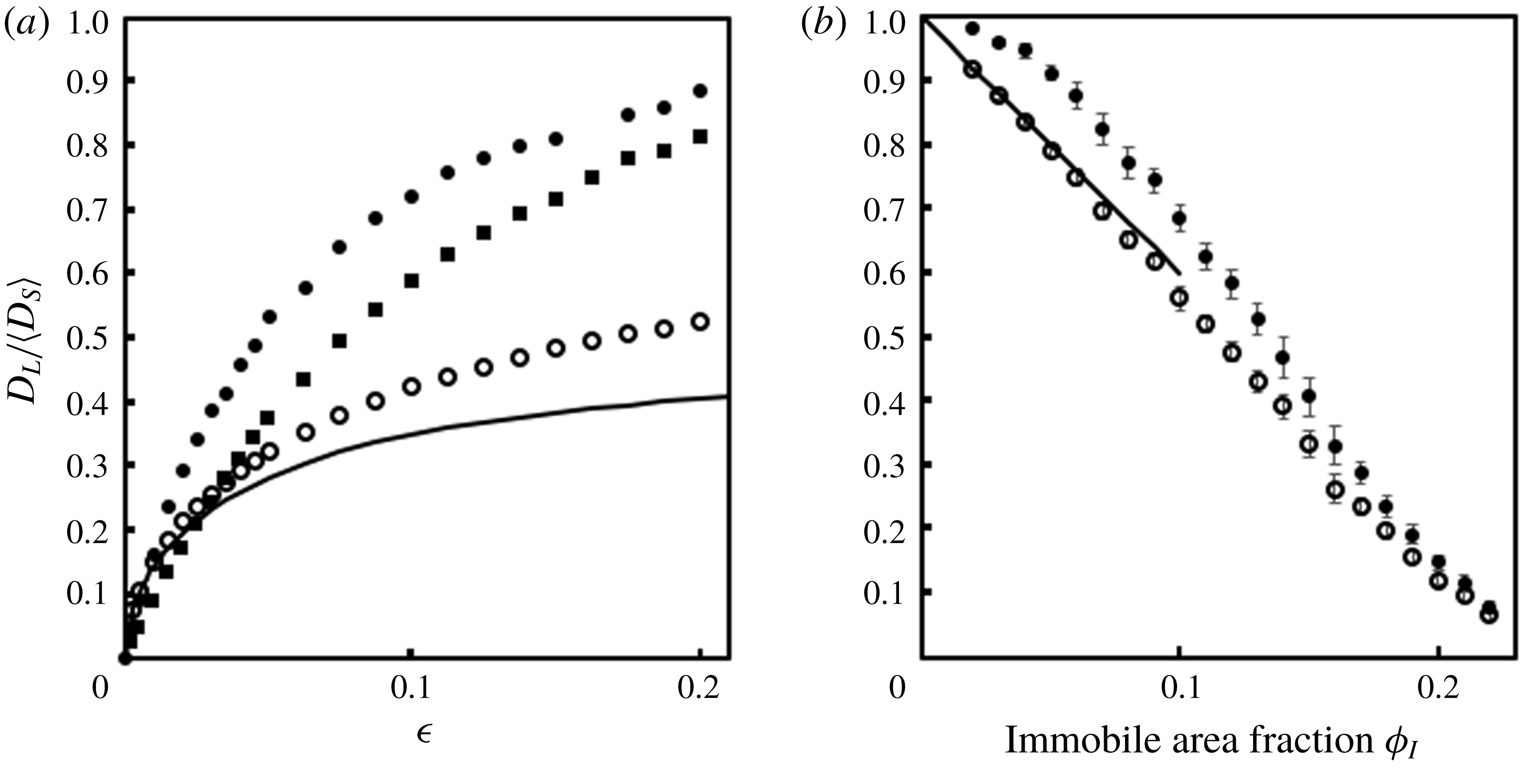
One hypothesis for the low rates of transmembrane protein diffusion that we will investigate here is the presence of transmembrane proteins in the plasma membrane which are immobilized by the actin cytoskeleton. Interactions between mobile proteins and immobile proteins may slow the diffusion of the mobile proteins. These interactions can be of two types: direct thermodynamic interactions between the proteins, and hydrodynamic interactions mediated through the intervening lipids in the membrane. Previous studies that treat only hydrodynamic interactions appear to be able to account for much of the observed decrease in diffusion rates in plasma membranes (Bussell, Koch & Hammer Reference Bussell, Koch and Hammer1995; Dodd et al. Reference Dodd, Hammer, Sangani and Koch1995), while those studies that treat only thermodynamic interactions also appear to account for a modest decrease in diffusion rates (Saxton Reference Saxton1987, Reference Saxton1990). However, no work thus far has rigorously combined both of these effects.
To study these interactions, a simplified model is often used in which the proteins are cylinders with radius
 $a$
and the lipid bilayer is a thin viscous fluid with viscosity
 $\unicode[STIX]{x1D707}$
and thickness
 $h$
. The aqueous phase surrounding the bilayer is a fluid with viscosity
 $\unicode[STIX]{x1D707}^{\prime }\ll \unicode[STIX]{x1D707}$
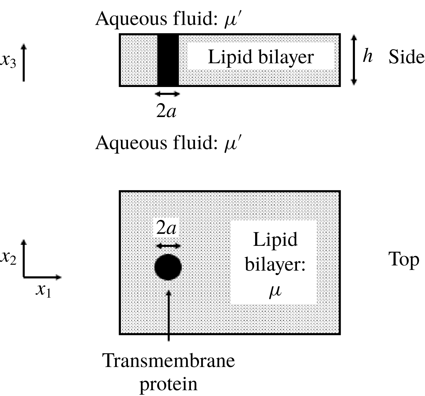
. Portions of the proteins that protrude into the aqueous fluid are neglected. These portions do not contribute significantly to hydrodynamic effects because they induce less stress on neighbouring proteins than the portions within the membrane. While these protruding portions may contribute significantly to thermodynamic effects, their shape is highly variable, and we choose to start with the simplest case, in which only the cylindrical portions within the membrane contribute to thermodynamic effects. In this work, the only thermodynamic effect we consider is excluded volume. Although the immobilized proteins are often only transiently immobilized, and remodelling of the cytoskeleton often changes the structure of the immobilized proteins, we will assume here that the immobile proteins are permanently immobilized in a static structure. This model is depicted in figure 1. Starting with this model, we attempt here to combine the hydrodynamic and thermodynamic effects of immobile proteins on the diffusion of mobile proteins.
Important features of a cell membrane. The cell membrane is a thin viscous fluid with cylindrically shaped proteins embedded within it. Side and top views of the same membrane are shown here. The lipids form a fluid with viscosity
 $\unicode[STIX]{x1D707}$
and thickness
 $h$
. The proteins have height
 $h$
and radius
 $a$
. The membrane is surrounded by a fluid with viscosity
 $\unicode[STIX]{x1D707}^{\prime }\ll \unicode[STIX]{x1D707}$
.

Some important results of previous studies of hydrodynamic interactions in cell membranes are worthy of mention here. Saffman & Delbrück (Reference Saffman and Delbrück1975) and Saffman (Reference Saffman1976) solved the Stokes equations for the self-mobility of a single cylindrical particle in an infinite viscous sheet. The self-mobility is the velocity with which a particle moves when acted upon by a force of unit magnitude. Because velocity disturbances due to a force acting on a two-dimensional (2-D) fluid do not decay (Stokes’ paradox), physical solutions for the self-mobility can only be attained by including information about the three-dimensional (3-D) environment in which the membrane is embedded. Saffman & Delbrück (Reference Saffman and Delbrück1975) did so by introducing the aqueous-phase viscosity
 $\unicode[STIX]{x1D707}^{\prime }$
on a length scale
 $\unicode[STIX]{x1D706}a$
, where
 $\unicode[STIX]{x1D706}=\unicode[STIX]{x1D707}h/(\unicode[STIX]{x1D707}^{\prime }a)$
is
 $O(10^{2}{-}10^{3})$
in a typical lipid bilayer. By modelling the fluid flow as strictly 2-D on a small length scale (
 $a$
) and including the 3-D flow in the aqueous phase on a larger length scale (
 $a\unicode[STIX]{x1D706}$
), and after asymptotically matching the two solutions, these authors showed that the diffusivity of the single cylinder is
 $$\begin{eqnarray}\displaystyle D_{0}(\unicode[STIX]{x1D706})=m_{0}k_{b}T=\frac{k_{b}T}{4\unicode[STIX]{x03C0}\unicode[STIX]{x1D707}h}[\ln \unicode[STIX]{x1D706}-\unicode[STIX]{x1D6FE}], & & \displaystyle\end{eqnarray}$$
where
 $m_{0}$
and
 $D_{0}$
are the self-mobility and self-diffusivity, respectively, in the limit of protein area fraction
 $\unicode[STIX]{x1D719}\rightarrow 0$
,
 $k_{b}$
is the Boltzmann constant,
 $T$
is temperature and
 $\unicode[STIX]{x1D6FE}$
is the Euler constant. The Einstein relation has been used here to compute the self-diffusivity from the self-mobility. Because of the simplicity of the interactions modelled here, the self-diffusivity is isotropic and independent of time.
The rotational diffusivity
 $D_{r,0}$
of one particle in an infinite domain is more straightforward because the velocity disturbance from a torque decays in two dimensions. The rotational mobility
 $m_{r,0}$
is the angular velocity of a particle when acted on by a torque of unit magnitude. Saffman (Reference Saffman1976) showed that the rotational diffusivity is
 $$\begin{eqnarray}\displaystyle D_{r,0}=m_{r,0}k_{b}T=\frac{k_{b}T}{4\unicode[STIX]{x03C0}\unicode[STIX]{x1D707}ha^{2}}. & & \displaystyle\end{eqnarray}$$
Others have built on these results to include hydrodynamic interactions between multiple particles. Bussell, Koch & Hammer (Reference Bussell, Koch and Hammer1992) found the short-time diffusivity of two mobile proteins in an infinite domain. Here, the diffusivity obtained from solving the Stokes equations is called a short-time diffusivity,
 $D_{s}$
, because it is valid on small time intervals when the changes in interparticle spacing are negligible. It accounts for hydrodynamic effects only. Bussell, Hammer & Koch (Reference Bussell, Hammer and Koch1994) used these results with ensemble averaging techniques to estimate the long-time diffusivity for all-mobile dilute suspensions. Dodd et al. (Reference Dodd, Hammer, Sangani and Koch1995) derived the hydrodynamic mobilities for randomly arranged cylinders in a periodic domain, used a novel method to match this result with an outer solution for a fully random unbounded array with aqueous-phase hydrodynamic interactions, and performed ensemble averages to provide accurate short-time diffusivities for non-dilute bilayers. In that work and here, non-overlapping random arrangements are obtained through Brownian dynamics simulation with hard-core potentials between the cylinders. The long-time diffusivity,
 $D_{L}$
, accounts for both the hydrodynamic and thermodynamic effects of other proteins. Brady (Reference Brady1994) used observations about the limiting behaviour of the short- and long-time diffusivities of all-mobile suspensions of spheres near their maximum packing fraction to propose that hydrodynamic effects do not change the ratio
 $D_{L}/D_{s}$
. This factorization, in which only hydrodynamic interactions affect
 $D_{s}$
and only thermodynamic interactions affect
 $D_{L}/D_{s}$
, appears to be in agreement with experimental literature on 3-D colloidal suspensions (Medina-Noyola Reference Medina-Noyola1988; Brady Reference Brady1994). In their calculation of the long-time diffusivity of transmembrane proteins in all-mobile membranes, Bussell et al. (Reference Bussell, Hammer and Koch1994) and Dodd et al. (Reference Dodd, Hammer, Sangani and Koch1995) made use of this relation by computing only hydrodynamic effects on
 $D_{s}$
and only thermodynamic effects on
 $D_{L}/D_{s}$
, and multiplying the results together. The thermodynamic effects in these works involved excluded volume only.
The hydrodynamic effect of immobilized proteins on mobile proteins has also been studied. This case is qualitatively different from the case of all-mobile suspensions because the immobile proteins form a fixed bed which causes velocity disturbances to decay (Brinkman Reference Brinkman1949). This decay occurs over a length scale
 $\unicode[STIX]{x1D706}_{B}a=a\unicode[STIX]{x1D719}_{I}^{-1/2}$
, where
 $\unicode[STIX]{x1D719}_{I}$
is the area fraction of immobile particles. At typical immobile area fractions in plasma membranes,
 $\unicode[STIX]{x1D706}_{B}$
is much smaller than
 $\unicode[STIX]{x1D706}$
, and interactions with the fixed bed are the primary mechanism for decay of velocity disturbances. Therefore, the aqueous-phase viscosity can be neglected under these conditions and fluid flows in the cell membrane can be treated as strictly 2-D. Biologically relevant area fractions of immobile proteins have been shown to decrease short-time self-diffusivities considerably (Bussell et al.
Reference Bussell, Koch and Hammer1995; Dodd et al.
Reference Dodd, Hammer, Sangani and Koch1995) and may account for the lower diffusivities observed in plasma membranes compared to reconstituted membranes that do not contain immobilized proteins. More recently, Oppenheimer & Diamant have presented theories for correlated diffusion between two mobile proteins in free-standing membranes (Oppenheimer & Diamant Reference Oppenheimer and Diamant2009), membranes near a solid substrate (Oppenheimer & Diamant Reference Oppenheimer and Diamant2010) and membranes with immobile inclusions (Oppenheimer & Diamant Reference Oppenheimer and Diamant2011). All of this previous work on partially immobile suspensions has treated hydrodynamic effects, and thus short-time diffusivity, only. A separate body of literature exists in which only thermodynamic effects on
 $D_{L}/D_{s}$
have been investigated (Saxton Reference Saxton1987, Reference Saxton1990; Nicolau, Hancock & Burrage Reference Nicolau, Hancock and Burrage2007; Niehaus et al.
Reference Niehaus, Vlachos, Edwards, Plechac and Tribe2008; Zhou Reference Zhou2009). Others have proposed that the same factorization into thermodynamic and hydrodynamic parts that Brady (Reference Brady1994) derived for the long-time diffusivity in all-mobile suspensions also holds for diffusion in fixed beds. Good agreement has been found between a 3-D effective medium theory which makes use of this factorization and experimental results for the diffusion of macromolecules in agarose gels (Johnson et al.
Reference Johnson, Berk, Jain and Deen1996). In the context of transmembrane protein diffusion, the effect of immobile proteins on the long-time self-diffusivity of mobile transmembrane proteins has been computed by assuming that this factorization is valid in partially mobile membranes. Bussell et al. (Reference Bussell, Koch and Hammer1995) and Dodd et al. (Reference Dodd, Hammer, Sangani and Koch1995) multiplied the short-time diffusivities they computed from hydrodynamic interactions only with ratios
 $D_{L}/D_{s}$
computed from thermodynamic interactions only. In the present study, it will be seen that this factorization is not accurate in partially mobile membranes, and indeed the conditions that led Brady (Reference Brady1994) to propose it in all-mobile 3-D suspensions do not apply to 2-D fixed beds.
Phillips, Deen & Brady (Reference Phillips, Deen and Brady1989) developed a rigorous method to study the long-time diffusivity of spherical macromolecules in a fibrous medium. In that work, a mobile sphere was placed in a periodic square lattice of immobilized spheres arranged as bead-and-string fibres. The short-time diffusivity of the mobile macromolecule at different positions within the unit cell was computed using the methods of Stokesian dynamics (Brady & Bossis Reference Brady and Bossis1988). These authors computed long-time diffusivities based on the short-time diffusivities using a formalism developed by Brenner (Reference Brenner1980) and adapted for mobile particles of non-zero size by Brenner & Adler (Reference Brenner and Adler1982). In this formalism, the probability density of a tracer particle within a spatially periodic porous medium is considered.
As part of a non-steady-state tracer analysis using the moments method of Aris (Reference Aris1956), Brenner (Reference Brenner1980) introduced a vector field,
 $\boldsymbol{B}$
, arising from a trial solution for the first-order moment of the probability density. For the specific case of no average fluid or tracer velocities,
 $\boldsymbol{B}$
can be interpreted physically by relating it to the concentration,
 $c$
, of tracers in the medium. A vector concentration field,
 $\boldsymbol{C}$
, can be defined by relating the concentration field to the average concentration gradient across the unit cell,
 $\unicode[STIX]{x1D735}\langle c\rangle$
:
 $$\begin{eqnarray}\displaystyle c=\boldsymbol{C}\boldsymbol{\cdot }\unicode[STIX]{x1D735}\langle c\rangle . & & \displaystyle\end{eqnarray}$$
Here, the angled brackets denote an ensemble average. Brenner (Reference Brenner1980) carried out a steady-state analysis of pure molecular diffusion in the same system and showed that
 $\boldsymbol{C}$
and
 $\boldsymbol{B}$
could be trivially related as follows:
 $$\begin{eqnarray}\displaystyle \boldsymbol{C}=-\boldsymbol{B}+\text{const}. & & \displaystyle\end{eqnarray}$$
Using this formalism, a concentration drop across the unit cell can be specified in terms of
 $\boldsymbol{B}$
. In the case of one mobile particle, as in Phillips et al. (Reference Phillips, Deen and Brady1989) or the present study, this concentration can be interpreted as the concentration of isolated non-interacting mobile particles. The concentration drop results in a flux of mobile particles across the unit cell, and Fick’s first law can be used to define and compute a long-time diffusivity for the isolated mobile particles. Phillips et al. (Reference Phillips, Deen and Brady1989) used this method to calculate the long-time diffusivity of a single spherical macromolecule in a square array of bead-and-string fibres as a function of the spacing between the fibres.
In this paper, we describe a method to combine hydrodynamic and thermodynamic effects to compute the long-time self-diffusivity of isolated mobile proteins in a square periodic unit cell with randomly arranged immobile proteins. We make use of a technique similar to that of Dodd et al. (Reference Dodd, Hammer, Sangani and Koch1995) to compute short-time diffusivities and the formalism developed by Phillips et al. (Reference Phillips, Deen and Brady1989) to use these short-time diffusivities to compute long-time diffusivities for a single mobile circular disk in a periodically replicated unit cell with immobile disks. Long-time diffusivities as a function of immobile area fraction for a relatively small system size are presented. We show that hydrodynamic interactions affect
 $D_{L}/D_{s}$
and that hydrodynamic and thermodynamic interactions must be computed together to accurately calculate
 $D_{L}$
. We also describe an approximate network analysis that can be used to calculate the long-time self-diffusivity for larger numbers of particles and thereby access diffusion properties close to a percolation threshold at
 $\unicode[STIX]{x1D719}_{I}\approx 0.22$
. This method is based on a suggestion by Sung & Yethiraj (Reference Sung and Yethiraj2006, Reference Sung and Yethiraj2008) in a study of transmembrane diffusion without hydrodynamic interactions in which the random array of immobile particles is replaced by a network of pores and bonds identified by Voronoi tessellation. We then use our rigorous diffusion calculation to estimate the resistance to diffusion through the gap between a pair of immobile proteins. The approximate method can then be used to accurately estimate long-time diffusivities for the large systems needed to approximate the diffusivity in an unbounded random array near the percolation threshold.
The organization of this paper is as follows. In § 2, we describe the scheme presented in Dodd et al. (Reference Dodd, Hammer, Sangani and Koch1995) to compute short-time diffusivities, but with modifications to describe near-field hydrodynamic interactions more conveniently. In § 3, we develop the method to compute long-time self-diffusivities (§ 3.1). After posing and solving a lubrication problem for the long-time diffusivity of a single mobile protein diffusing through a small gap between two immobile proteins (§ 3.2), we present long-time self-diffusivities for isolated mobile proteins diffusing in square arrays of immobile proteins for different unit-cell sizes and show their correspondence to the lubrication result (§ 3.3). We then turn to random arrays of immobile proteins. First, the approximate network method is described in § 4. In § 5, we use the finite element method (FEM)/multipole calculations and network analysis to compute the long-time diffusivity in arrays with a range of unit-cell sizes and eventually estimate the long-time diffusivity as a function of immobile area fraction in infinite arrays of immobile proteins. In § 6, we show that the finite-size scaling of the long-time self-diffusivity near the percolation threshold appears to be consistent with the prediction from percolation theory. Finally, in § 7, we show that the ratio of the long-time self-diffusivity to the spatially averaged short-time self-diffusivity is significantly higher in the presence of hydrodynamic interactions, invalidating the previously held assumption that hydrodynamic and thermodynamic interactions can be computed separately in these suspensions. In the conclusion (§ 8), we discuss some implications of our results and possible applications of the methods introduced here to the study of transmembrane protein diffusion.
2 Computation of short-time diffusivity
To compute short-time diffusivities, we must first calculate hydrodynamic interactions between an arbitrary arrangement of
 $N$
cylinders of equal size immersed in a thin viscous sheet with periodic boundary conditions. In this work,
 $N_{p}\leqslant N$
cylinders are mobile, while the remaining cylinders are considered immobile. All cylinders are rigid. We compute short-time diffusivities in a manner similar to Dodd et al. (Reference Dodd, Hammer, Sangani and Koch1995). We start with a truncated multipole expansion using the method of Sangani & Yao (Reference Sangani and Yao1988) and add near-field interactions to the resulting resistance matrix. Our scheme for adding near-field interactions differs from that of Dodd et al. (Reference Dodd, Hammer, Sangani and Koch1995), but the multipole expansion scheme is the same. Nevertheless, we present both parts of the method here for clarity and completeness. Our method treats both translational and rotational motion. However, we only discuss translational diffusion in subsequent sections because our newer methods do not add to the understanding of rotational diffusion put forth in Dodd et al. (Reference Dodd, Hammer, Sangani and Koch1995).
2.1 Multipole expansion
To describe the multipole expansion technique, we closely follow the treatment of Sangani & Yao (Reference Sangani and Yao1988). The governing equations are
 $$\begin{eqnarray}\displaystyle \unicode[STIX]{x1D735}p=\unicode[STIX]{x1D707}\unicode[STIX]{x1D6FB}^{2}\boldsymbol{u}, & & \displaystyle\end{eqnarray}$$
 $$\begin{eqnarray}\displaystyle \unicode[STIX]{x1D735}\boldsymbol{\cdot }\boldsymbol{u}=0, & & \displaystyle\end{eqnarray}$$
where
 $p$
is pressure,
 $\unicode[STIX]{x1D707}$
is viscosity and
 $\boldsymbol{u}$
is the velocity of the fluid. We will assume a no-slip boundary condition on the surface of each disk. This can be written as
 $$\begin{eqnarray}\displaystyle \left.\begin{array}{@{}ll@{}}\displaystyle \frac{1}{2\unicode[STIX]{x03C0}}\int _{0}^{2\unicode[STIX]{x03C0}}\boldsymbol{u}\text{e}^{\text{i}l\unicode[STIX]{x1D703}}\,\text{d}\unicode[STIX]{x1D703}=\boldsymbol{C}(l), & \quad \text{on}~\unicode[STIX]{x2202}D^{(s)},~s=1,2,\ldots ,N,\\ \boldsymbol{C}(l)=\boldsymbol{U}^{(s)}, & \quad \text{for}~l=0,\\ \phantom{\boldsymbol{C}(l)}=\frac{1}{2}(a\unicode[STIX]{x1D714}^{(s)})(1\,\boldsymbol{e}_{\boldsymbol{ 2}}-\text{i}\,\boldsymbol{e}_{\mathbf{1}}), & \quad \text{for}~l=1,\\ \phantom{\boldsymbol{C}(l)}=\mathbf{0}, & \quad \text{for}~l\geqslant 2.\end{array}\right\} & & \displaystyle\end{eqnarray}$$
Here,
 $\unicode[STIX]{x2202}D^{(s)}$
is the surface of disk
 $s$
,
 $\boldsymbol{U}^{(s)}$
its linear velocity and
 $\unicode[STIX]{x1D74E}^{(s)}=\unicode[STIX]{x1D714}^{(s)}\boldsymbol{e}_{\mathbf{3}}$
its angular velocity; and
 $\boldsymbol{e}_{\mathbf{1}}$
,
 $\boldsymbol{e}_{\mathbf{2}}$
and
 $\boldsymbol{e}_{\mathbf{3}}$
are orthonormal basis vectors in a Cartesian coordinate system. We assume that thermodynamic considerations restrict the orientation of the cylinders in the bilayer so that their longitudinal axes align with the bilayer normal. We can solve for the velocity components and the pressure in terms of the periodic Green’s functions
 $S_{1}$
and
 $S_{2}$
:
 $$\begin{eqnarray}\displaystyle & \displaystyle u_{1}=U_{1}+\mathop{\sum }_{s=1}^{N}\left[B_{00}^{(s)}\frac{\unicode[STIX]{x2202}S_{1}}{\unicode[STIX]{x2202}x_{2}}+\mathop{\sum }_{n=1}^{\infty }\mathop{\sum }_{m=0}^{1}\left(A_{nm}^{(s)}\frac{\unicode[STIX]{x2202}^{n+1}S_{2}}{\unicode[STIX]{x2202}x_{1}^{n-m}\unicode[STIX]{x2202}x_{2}^{m+1}}+B_{nm}^{(s)}\frac{\unicode[STIX]{x2202}^{n+1}S_{1}}{\unicode[STIX]{x2202}x_{1}^{n-m}\unicode[STIX]{x2202}x_{2}^{m+1}}\right)\right], & \displaystyle\end{eqnarray}$$
 $$\begin{eqnarray}\displaystyle & \displaystyle u_{2}=U_{2}-\mathop{\sum }_{s=1}^{N}\left[B_{00}^{(s)}\frac{\unicode[STIX]{x2202}S_{1}}{\unicode[STIX]{x2202}x_{1}}+\mathop{\sum }_{n=1}^{\infty }\mathop{\sum }_{m=0}^{1}\left(A_{nm}^{(s)}\frac{\unicode[STIX]{x2202}^{n+1}S_{2}}{\unicode[STIX]{x2202}x_{1}^{n-m+1}\unicode[STIX]{x2202}x_{2}^{m}}+B_{nm}^{(s)}\frac{\unicode[STIX]{x2202}^{n+1}S_{1}}{\unicode[STIX]{x2202}x_{1}^{n-m+1}\unicode[STIX]{x2202}x_{2}^{m}}\right)\right], & \displaystyle\end{eqnarray}$$
 $$\begin{eqnarray}\displaystyle & \displaystyle \frac{1}{\unicode[STIX]{x1D707}}p=\mathop{\sum }_{s=1}^{N}\left[A_{11}^{(s)}\left(\frac{4\unicode[STIX]{x03C0}x_{1}}{L^{2}}-\frac{\unicode[STIX]{x2202}S_{1}}{\unicode[STIX]{x2202}x_{1}}\right)+A_{10}^{(s)}\left(\frac{-4\unicode[STIX]{x03C0}x_{2}}{L^{2}}+\frac{\unicode[STIX]{x2202}S_{1}}{\unicode[STIX]{x2202}x_{2}}\right)+\mathop{\sum }_{n=2}^{\infty }\mathop{\sum }_{m=0}^{1}A_{nm}^{(s)}\frac{\unicode[STIX]{x2202}^{n}S_{1}}{\unicode[STIX]{x2202}x_{1}^{n-m-1}\unicode[STIX]{x2202}x_{2}^{m+1}}\right]. & \displaystyle \nonumber\\ \displaystyle & & \displaystyle\end{eqnarray}$$
Here
 $U_{1}$
and
 $U_{2}$
are the components of the mean fluid velocity;
 $A_{nm}$
and
 $B_{nm}$
are coefficients to be determined through the boundary conditions; and
 $L$
is the size of the unit cell, which is assumed to be square here. Finally,
 $S_{1}$
and
 $S_{2}$
are evaluated at
 $\boldsymbol{x}=\boldsymbol{R}^{(s)}$
;
 $S_{1}$
and
 $S_{2}$
were first defined by Hasimoto (Reference Hasimoto1959) as
 $$\begin{eqnarray}\displaystyle S_{m}(\boldsymbol{x})=\frac{1}{\unicode[STIX]{x03C0}L^{2}(-4\unicode[STIX]{x03C0}^{2})^{m-1}}\mathop{\sum }_{\boldsymbol{k}\neq \mathbf{0}}k^{-2m}\exp (2\unicode[STIX]{x03C0}\text{i}\boldsymbol{k}\boldsymbol{\cdot }\boldsymbol{x}),\quad m=1,2. & & \displaystyle\end{eqnarray}$$
One can solve a Stokes flow problem in the resistance formulation by substituting (2.4) and (2.5) into (2.3) with a given set of velocities and angular velocities for the cylinders, and then solving for the coefficients
 $A_{nm}$
and
 $B_{nm}$
. We provide more details for this procedure in appendix A. The coefficients are related to the force density moments on the cylinders. The forces and torques on the disks are given by
 $$\begin{eqnarray}\displaystyle & \displaystyle F_{1}^{(s)}=-4\unicode[STIX]{x03C0}\unicode[STIX]{x1D707}A_{11}^{(s)}, & \displaystyle\end{eqnarray}$$
 $$\begin{eqnarray}\displaystyle & \displaystyle F_{2}^{(s)}=4\unicode[STIX]{x03C0}\unicode[STIX]{x1D707}A_{10}^{(s)}, & \displaystyle\end{eqnarray}$$
 $$\begin{eqnarray}\displaystyle & \displaystyle L_{3}^{(s)}=-4\unicode[STIX]{x03C0}\unicode[STIX]{x1D707}(2B_{00}^{(s)}+A_{20}^{(s)}). & \displaystyle\end{eqnarray}$$
Both the expressions for the velocity and the boundary condition can be truncated to yield a finite set of equations with an equal number of unknowns. We limit the infinite sum over
 $n$
in (2.4) and (2.5) to
 $n\leqslant n_{s}$
, and we limit the values of
 $l$
in (2.3) to
 $l\leqslant n_{s}$
. Thus, the forces and torques on each cylinder can be found by solving this finite set of linear equations, and the accuracy of the calculation increases with
 $n_{s}$
.
The forces and torques on just the mobile particles can then be found for each problem in which only one (mobile) particle experiences translational or rotational motion (a total of
 $3N_{p}$
problems). These couplings can be combined into a resistance matrix
 $\unicode[STIX]{x1D64D}$
:
 $$\begin{eqnarray}\displaystyle \left[\begin{array}{@{}c@{}}\boldsymbol{F}\\ \boldsymbol{ L}\end{array}\right]=-\unicode[STIX]{x1D64D}\boldsymbol{\cdot }\left[\begin{array}{@{}c@{}}\boldsymbol{U}\\ \unicode[STIX]{x1D74E}\end{array}\right]. & & \displaystyle\end{eqnarray}$$
Here,
 $\boldsymbol{F}$
are the forces on the mobile particles only,
 $\boldsymbol{L}$
are the torques on the mobile particles,
 $\boldsymbol{U}$
are the translational velocities and
 $\unicode[STIX]{x1D74E}$
are the angular velocities. Matrix
 $\unicode[STIX]{x1D64D}$
is a
 $3N_{p}\times 3N_{p}$
matrix. Its inverse is the mobility matrix:
 $$\begin{eqnarray}\displaystyle \unicode[STIX]{x1D648}=\unicode[STIX]{x1D64D}^{-1}. & & \displaystyle\end{eqnarray}$$
2.2 Near-field interactions
To reduce computational cost, we choose
 $n_{s}=4$
as in Dodd et al. (Reference Dodd, Hammer, Sangani and Koch1995). However, these calculations can be inaccurate for small interparticle distances. We correct for this in a different manner than that in Dodd et al. (Reference Dodd, Hammer, Sangani and Koch1995). We explicitly add forces and torques from near-field two-particle interactions between particles with separations smaller than a specified cutoff distance to the resistance matrix. We set this cutoff distance at
 $2.4a$
. For two particles in a force-free suspension, there are three independent couplings for translational motion (force from normal motion, force from tangential motion, and torque from tangential motion) and three independent couplings for rotational motion (torque on the rotating particle, torque on the non-rotating particle, and the force on either particle). The torque from tangential motion is equivalent to the force from rotation according to the Lorentz reciprocal theorem, giving five independent couplings. In addition, the torque on the non-rotating particle from rotation of the other particle does not exhibit lubrication scaling. We compared the values of the remaining four couplings for two particles in a unit cell of size
 $10\,000a$
for different interparticle distances between
 $n_{s}=4$
and
 $n_{s}=50$
. At an interparticle distance of
 $2.4a$
, the maximum deviation from the
 $n_{s}=50$
results, which we consider exact, is 2.48 % for the force from normal motion. The deviation for the non-lubrication coupling (torque on one particle from rotation of the second) at that distance is 5.75 %. We therefore chose
 $2.4a$
as the cutoff distance to include near-field interactions as in Dodd et al. (Reference Dodd, Hammer, Sangani and Koch1995).
When particles are separated by a distance less than
 $2.4a$
, we add near-field contributions pairwise to the existing values in the resistance matrix as follows. All of the couplings discussed above for two particles were computed and tabulated for
 $n_{s}=50$
and
 $n_{s}=4$
for a unit-cell size of
 $10\,000a$
for interparticle distances between
 $2.01a$
and
 $2.40a$
in increments of
 $0.01a$
. The lubrication scalings of these couplings with half-gap distance
 $\unicode[STIX]{x1D716}$
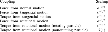
, first reported by Bussell et al. (Reference Bussell, Koch and Hammer1992), are shown in table 1. Additional near-field contributions to the resistance matrix were calculated by using the lubrication scalings to interpolate between the
 $n_{s}=50$
tabulated values and subtracting a linear interpolation of the
 $n_{s}=4$
tabulated values. These additional near-field terms are then added to the many-body
 $n_{s}=4$
values from the multipole expansion. For the torque on a stationary particle from rotation of another particle, a linear interpolation was used. In our implementation, a separate near-field resistance matrix is added to the resistance matrix computed from the
 $n_{s}=4$
multipole expansion:
 $$\begin{eqnarray}\displaystyle \unicode[STIX]{x1D64D}=\unicode[STIX]{x1D64D}_{4}+\unicode[STIX]{x1D64D}_{nf}. & & \displaystyle\end{eqnarray}$$
Here,
 $\unicode[STIX]{x1D64D}_{4}$
is the many-body resistance matrix computed from the multipole expansion with
 $n_{s}=4$
, and
 $\unicode[STIX]{x1D64D}_{nf}$
is the additional near-field contribution to the resistance matrix. A detailed example of the near-field contribution can be given for one particular element of the matrix. The force,
 $F_{N}$
, resulting from normal relative motion of nearby particles is
 $$\begin{eqnarray}\displaystyle F_{N}=F_{4}+F_{nf}, & & \displaystyle\end{eqnarray}$$
 $$\begin{eqnarray}\displaystyle F_{nf} & = & \displaystyle \frac{\unicode[STIX]{x1D716}^{-3/2}}{0.01(\frac{1}{2})a}\,f_{50}(0.01a)-f_{4}(0.01a)\quad \text{for}~2\unicode[STIX]{x1D716}<0.01a,\nonumber\\ \displaystyle & = & \displaystyle f_{50}(2\unicode[STIX]{x1D716})-f_{4}(2\unicode[STIX]{x1D716})\quad \text{for}~0.01a<2\unicode[STIX]{x1D716}\leqslant 0.40a~\text{and}~2\unicode[STIX]{x1D716}-\lfloor 2\unicode[STIX]{x1D716}\rfloor <10^{-5},\nonumber\\ \displaystyle & = & \displaystyle \frac{\unicode[STIX]{x1D716}^{-3/2}-(\frac{1}{2}\lceil 2\unicode[STIX]{x1D716}\rceil )^{-3/2}}{(0.005a)^{-3/2}}[f_{50}(\lfloor 2\unicode[STIX]{x1D716}\rfloor )-f_{50}(\lceil 2\unicode[STIX]{x1D716}\rceil )]\nonumber\\ \displaystyle & & \displaystyle -\left[\frac{\unicode[STIX]{x1D716}-(\frac{1}{2}\lceil 2\unicode[STIX]{x1D716}\rceil )}{(0.005a)}(f_{4}(\lfloor 2\unicode[STIX]{x1D716}\rfloor )-f_{4}(\lceil 2\unicode[STIX]{x1D716}\rceil ))+f_{4}(\lfloor 2\unicode[STIX]{x1D716}\rfloor )\right]\nonumber\\ \displaystyle & & \displaystyle \qquad \qquad \qquad \qquad \text{for}~0.01a<2\unicode[STIX]{x1D716}\leqslant 0.40a~\text{and}~2\unicode[STIX]{x1D716}-\lfloor 2\unicode[STIX]{x1D716}\rfloor \geqslant 10^{-5}.\end{eqnarray}$$
Here,
 $F_{4}$
is the result from the multipole expansion with
 $n_{s}=4$
,
 $F_{nf}$
is the additional near-field contribution addressed in this section,
 $\unicode[STIX]{x1D716}$
is the half-gap width,
 $f_{50}(d)$
is the tabulated lubrication force for
 $n_{s}=50$
at a full gap width
 $d$
, and
 $f_{4}(d)$
is the tabulated lubrication force for
 $n_{s}=4$
at a full gap width
 $d$
. The symbols
 $\lfloor ~\rfloor$
and
 $\lceil ~\rceil$
denote the floor and ceiling functions, respectively.
Lubrication scaling of different resistance couplings with respect to half-gap distance
 $\unicode[STIX]{x1D716}$
for two cylinders of equal size in a force-free suspension. Adapted from Bussell et al. (Reference Bussell, Koch and Hammer1992).

The resistance matrix is inverted to find the mobility after including near-field forces and torques. The Einstein relation can then be used to compute the short-time diffusivities of the mobile particles. This method for including near-field interactions differs from the method in Dodd et al. (Reference Dodd, Hammer, Sangani and Koch1995). In that method, near-field interactions are included in two ways. First, additional forces and torques are calculated from the relevant lubrication problems. Second, a correction to the fluid flow is calculated by adding lubrication multipoles centred in the middle of the gap between two particles. The portion of the particle surfaces over which the force density is integrated in the lubrication problems is a fitting parameter and is different for each lubrication problem. We sought to avoid the use of fitting parameters in our method. In addition, the lubrication correction to the fluid flow gives resistance and mobility matrices that are not symmetric. While this asymmetry does not appear to be consequential for the work presented in Dodd et al. (Reference Dodd, Hammer, Sangani and Koch1995) or here, a symmetric mobility matrix is convenient for use in Brownian dynamics simulations because it can be easily interpreted as a variance–covariance matrix in the relation between viscous dissipation and Brownian forces arising from the fluctuation–dissipation theorem (Ermak & McCammon Reference Ermak and McCammon1978). For these reasons, we chose a different method to include near-field interactions which we believe to be accurate.
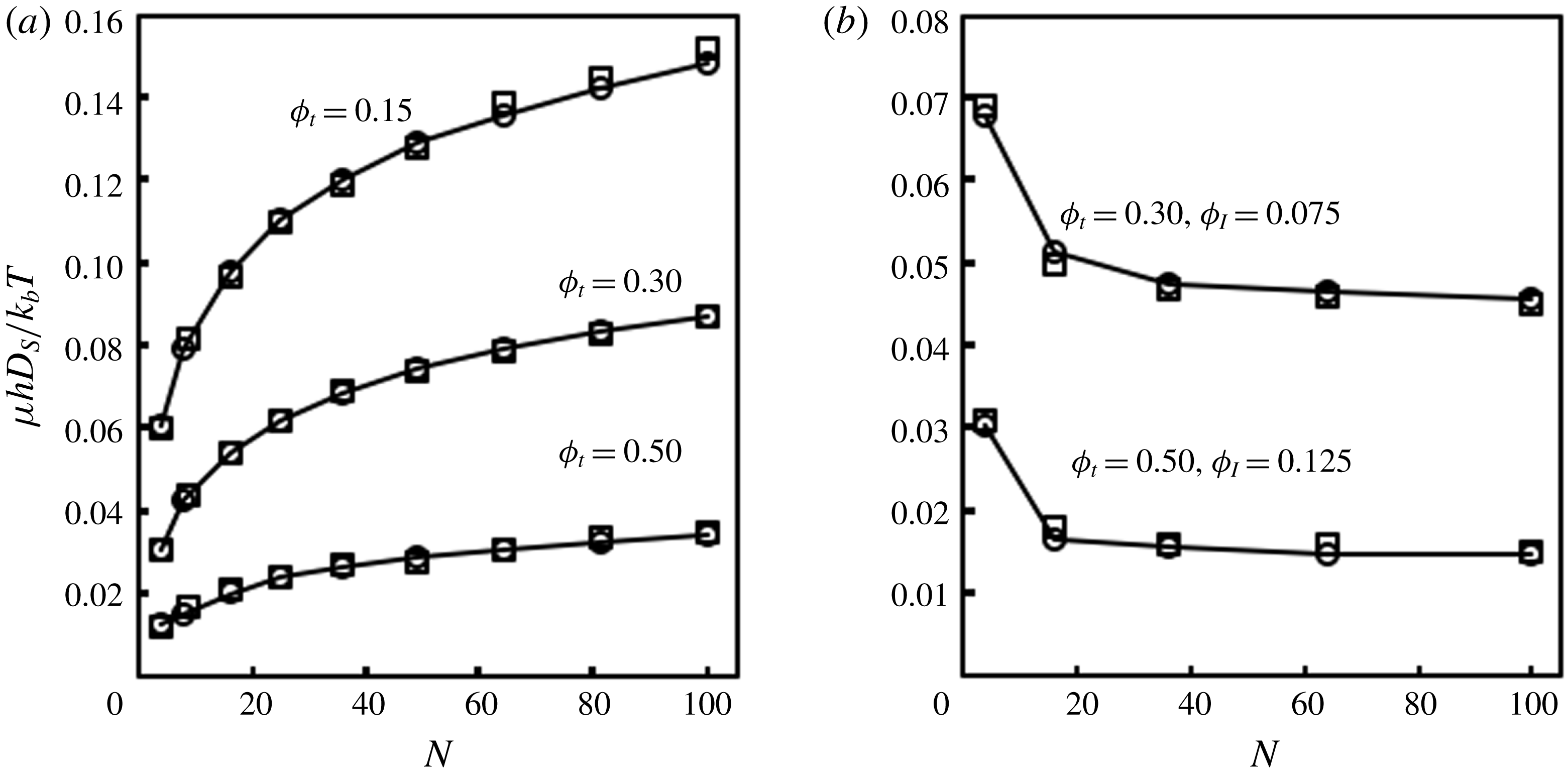
Figure 2 shows a comparison of ensemble-averaged short-time self-diffusivities calculated using our method with results from Dodd et al. (Reference Dodd, Hammer, Sangani and Koch1995). These short-time self-diffusivities were computed by generating random arrays of disks with the indicated numbers of disks at the indicated area fractions, calculating the short-time diffusivity matrix for the mobile disks in each configuration, and averaging over all of the translational self-diffusivities (the diagonal elements of the portion of the matrix which gives couplings for translational motion). At least
 $100$
configurations were used for each condition. Figure 2(a) shows computed short-time self-diffusivities for all-mobile suspensions as a function of the number of particles,
 $N$
, for different total particle area fractions,
 $\unicode[STIX]{x1D719}_{t}$
. The graphs show the expected logarithmic dependence on
 $N$
and close agreement between our results and those of Dodd et al. (Reference Dodd, Hammer, Sangani and Koch1995). While these computed self-diffusivities are not easily interpretable as shown, Dodd et al. (Reference Dodd, Hammer, Sangani and Koch1995) developed an effective medium theory which gives simple algebraic relations to renormalize them to include the effects of the aqueous-phase viscosity. The renormalized mobilities are applicable to reconstituted vesicles, in which there are no immobilized transmembrane proteins. Figure 2(b) shows short-time self-diffusivities for suspensions with differing total area fractions and immobile area fractions,
 $\unicode[STIX]{x1D719}_{I}$
, as shown. Again, close agreement between our results and those of Dodd et al. (Reference Dodd, Hammer, Sangani and Koch1995) is seen. The computed self-diffusivities approach a constant value for large
 $N$
. This is because, as previously noted, Brinkman screening in the presence of immobile proteins allows these strictly 2-D computations to be readily interpretable physically. There appears to be significant unit-cell size dependence for
 $N<25$
. To avoid this dependence, we restrict all hydrodynamic calculations in this work to unit cells with
 $N>25$
except in our finite-size analysis in figure 11. We now proceed to use this multipole calculation as part of a new method to compute long-time diffusivities for mobile transmembrane proteins.
Comparison of short-time self-diffusivity to results from Dodd et al. (Reference Dodd, Hammer, Sangani and Koch1995). Results from the current method are open circles, and results from Dodd et al. (Reference Dodd, Hammer, Sangani and Koch1995) are open squares. (a) Short-time diffusivities versus total number of disks for all-mobile suspensions at different total area fractions. (b) Short-time diffusivities versus total number of disks for partially immobilized suspensions.

3 Finite element method to compute long-time diffusivity
3.1 Finite element method
To calculate the long-time diffusivity of one mobile disk in an array of immobile disks in a square unit cell, we closely follow the treatment of Phillips et al. (Reference Phillips, Deen and Brady1989), in which the transport properties of a spherical particle in a square lattice of bead-and-string fibres were investigated. We consider the vector field
 $\boldsymbol{B}$
, introduced by Brenner (Reference Brenner1980), allowing us to represent a mean concentration gradient for the concentration of isolated mobile disks. For a system with only hard-core interactions, at steady state, when the average fluid and particle velocities are zero, the long-time diffusivity can be computed by solving the following equation for
 $\boldsymbol{B}$
:
 $$\begin{eqnarray}\displaystyle \unicode[STIX]{x1D735}\boldsymbol{\cdot }(\unicode[STIX]{x1D63F}_{\boldsymbol{s}}(\boldsymbol{x})\boldsymbol{\cdot }\unicode[STIX]{x1D735}\boldsymbol{B})=\mathbf{0}, & & \displaystyle\end{eqnarray}$$
with boundary conditions
 $$\begin{eqnarray}\displaystyle [[\boldsymbol{B}]]=-[[\boldsymbol{x}]]\quad \text{and}\quad [[\unicode[STIX]{x1D735}\boldsymbol{B}]]=\mathbf{0}, & & \displaystyle\end{eqnarray}$$
on the boundaries of the unit cell in the fluid, where the double-bracket symbol
 $[[~]]$
denotes the difference between the values of its argument at equivalent positions at opposite sides of the periodic unit cell, and
 $$\begin{eqnarray}\displaystyle \boldsymbol{n}\boldsymbol{\cdot }\unicode[STIX]{x1D63F}_{\boldsymbol{s}}(\boldsymbol{x})\boldsymbol{\cdot }\unicode[STIX]{x1D735}\boldsymbol{B}=\mathbf{0}, & & \displaystyle\end{eqnarray}$$
on the excluded-volume surface of the immobile disks. The excluded-volume surface is the surface of mobile particle centres when the mobile particle is in contact with an immobile particle. Here,
 $\boldsymbol{n}$
is a unit normal vector pointing into the accessible part of the unit cell,
 $\boldsymbol{x}$
is a vector specifying position within a unit cell, and
 $\unicode[STIX]{x1D63F}_{\boldsymbol{s}}(\boldsymbol{x})$
is the short-time diffusivity for a single mobile particle located at
 $\boldsymbol{x}$
within the fluid, computed as described in the previous section. The condition (3.2a,b
) applies a specified spatially averaged concentration gradient (of unit magnitude) across the unit cell. After solving this equation for
 $\boldsymbol{B}$
throughout the unit cell, described below, the long-time diffusivity tensor,
 $\unicode[STIX]{x1D63F}_{\boldsymbol{L}}$
, can be computed from Fick’s law. Adapting the treatment of Brenner (Reference Brenner1980) to particles of non-zero size, equations (1.3) and (1.4) can be used to calculate the local flux,
 $\boldsymbol{q}$
, of mobile disks as
 $$\begin{eqnarray}\displaystyle \boldsymbol{q}(\boldsymbol{x})=\unicode[STIX]{x1D63F}_{\boldsymbol{s}}\boldsymbol{\cdot }(\unicode[STIX]{x1D735}\boldsymbol{B})\boldsymbol{\cdot }\unicode[STIX]{x1D735}\langle c\rangle . & & \displaystyle\end{eqnarray}$$
A spatially averaged flux,
 $\langle \boldsymbol{q}\rangle$
, can be computed from this local flux:
 $$\begin{eqnarray}\displaystyle \langle \boldsymbol{q}\rangle =-\frac{1}{A_{f}}\int _{\boldsymbol{\unicode[STIX]{x2202}}\boldsymbol{x}_{\mathbf{0}}}\text{d}s\,\boldsymbol{n}\boldsymbol{\cdot }\boldsymbol{q}\boldsymbol{B}. & & \displaystyle\end{eqnarray}$$
Here,
 $A_{f}$
is the area of the unit cell that is accessible to the mobile particle and the integral is carried out around the excluded-volume surface of the disks and the boundaries of the unit cell (
 $\boldsymbol{\unicode[STIX]{x2202}}\boldsymbol{x}_{\mathbf{0}}$
). The differential
 $\text{d}s$
is the scalar arclength along
 $\boldsymbol{\unicode[STIX]{x2202}}\boldsymbol{x}_{\mathbf{0}}$
. The divergence theorem and a vector identity invoking the conservation of flux at steady state then give the following expression for the spatially averaged flux:
 $$\begin{eqnarray}\displaystyle \langle \boldsymbol{q}\rangle =-\frac{1}{A_{f}}\int _{\boldsymbol{x}_{\mathbf{0}}}(\unicode[STIX]{x1D735}\boldsymbol{B})^{\text{t}}\boldsymbol{\cdot }\unicode[STIX]{x1D63F}_{\boldsymbol{s}}(\boldsymbol{x})\boldsymbol{\cdot }(\unicode[STIX]{x1D735}\boldsymbol{B})\,\text{d}\boldsymbol{x}\boldsymbol{\cdot }\unicode[STIX]{x1D735}\langle c\rangle . & & \displaystyle\end{eqnarray}$$
Here, the integral is over the area of one unit cell. Now, Fick’s law allows us to define a long-time diffusivity by relating the spatially averaged flux to the spatially averaged concentration gradient:
 $$\begin{eqnarray}\displaystyle \langle \boldsymbol{q}\rangle =-\unicode[STIX]{x1D63F}_{\boldsymbol{L}}\boldsymbol{\cdot }\unicode[STIX]{x1D735}\langle c\rangle . & & \displaystyle\end{eqnarray}$$
This results in the following expression for
 $\unicode[STIX]{x1D63F}_{\boldsymbol{L}}$
, which is a limiting case of the expression presented by Brenner & Adler (Reference Brenner and Adler1982) for continuous-phase transport only:
 $$\begin{eqnarray}\displaystyle \unicode[STIX]{x1D63F}_{\boldsymbol{L}}=\frac{1}{A_{f}}\int _{\boldsymbol{x}_{\mathbf{0}}}(\unicode[STIX]{x1D735}\boldsymbol{B})^{\text{t}}\boldsymbol{\cdot }\unicode[STIX]{x1D63F}_{\boldsymbol{s}}(\boldsymbol{x})\boldsymbol{\cdot }(\unicode[STIX]{x1D735}\boldsymbol{B})\,\text{d}\boldsymbol{x}. & & \displaystyle\end{eqnarray}$$
Equation (3.8) weights the short-time diffusivities by their corresponding concentration gradients. This is different from a simple spatial average over the short-time diffusivities and accounts for the excluded-volume effects of the immobile disks in addition to their hydrodynamic effects, which are already included in
 $\unicode[STIX]{x1D63F}_{\boldsymbol{s}}$
. As Phillips et al. (Reference Phillips, Deen and Brady1989) explain, the FEM is convenient to solve the differential equation for
 $\boldsymbol{B}$
because the no-flux condition on the immobile particle surfaces given by (3.3) is easy to implement. An element will automatically satisfy this condition unless another boundary condition is explicitly specified. We solve (3.1) using a Galerkin FEM with linear basis functions for triangular elements.
We first used this method to compute the long-time diffusivity of isolated mobile disks in square arrays of immobilized disks. Because of the simple geometry of square periodic arrays, they facilitate quick and easy comparison to a lubrication problem for the long-time diffusivity of a mobile disk diffusing in a small gap between two immobile disks. Such a comparison would confirm that our FEM correctly captures the basic physics we seek to study. Therefore, before describing these FEM results, we introduce and solve this lubrication problem. We then compare this result to the FEM results for square arrays.
3.2 Lubrication problem
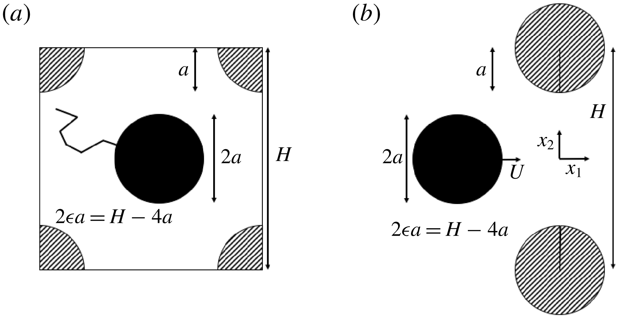
We carried out a lubrication analysis for a system similar to the square array to compare to FEM results for small unit-cell sizes. The square array system, discussed in the next section, is shown in figure 3(a). A mobile disk of radius
 $a$
diffuses through gaps between immobile disks of the same radius arranged in a square array in a 2-D viscous fluid. The centre-to-centre distance between the immobile disks is
 $H$
, and a non-dimensional half-gap
 $\unicode[STIX]{x1D716}$
is defined such that
 $2\unicode[STIX]{x1D716}a=H-4a$
. For
 $\unicode[STIX]{x1D716}\ll 1$
, we can carry out a lubrication analysis of this configuration by considering only the two immobile disks closest to the mobile disk. Because those two disks exhibit the most profound resistive effect on the mobile disk, such a theoretical analysis would give the correct leading-order behaviour for the long-time diffusivity, which we could then compare to the FEM results. The simplified system used for the lubrication analysis is shown in figure 3(b). Here, a mobile disk diffuses through a gap between two immobile disks, with
 $H$
and
 $\unicode[STIX]{x1D716}$
defined analogously to the system in figure 3(a). The origin of the coordinate system is at the middle of the gap.
Square array and lubrication geometry. (a) Unit cell for FEM computations on square arrays. A mobile disk (shown in solid black) diffuses through a square array of immobile disks (shown with hatched pattern). The unit cell has size
 $H$
and all disks have radius
 $a$
. (b) Geometry for lubrication problem. A mobile disk (shown in solid black) moves with velocity
 $U$
through a small gap between two immobile disks (shown with hatched pattern). All disks have radius
 $a$
and the centre-to-centre distance between the immobile disks is
 $H$
. A half-gap
 $\unicode[STIX]{x1D716}$
is defined such that
 $2\unicode[STIX]{x1D716}a=H-4a$
.

To simplify the analysis, we will consider a mobile disk that translates through the gap without rotation. If the mobile disk has velocity
 $\boldsymbol{U}=U\boldsymbol{e}_{\mathbf{1}}$
as shown, and if
 $\unicode[STIX]{x1D716}\ll 1$
, then lubrication results from Bussell et al. (Reference Bussell, Koch and Hammer1992) can be used to estimate the force of the fluid on it. The force of the fluid on the mobile disk can be used to estimate
 $D_{s11}$
, the component of the short-time diffusivity from coupling of a force in
 $x_{1}$
to a velocity in
 $x_{1}$
. This is the only component relevant for the leading-order behaviour. It is given to
 $O(\unicode[STIX]{x1D716}^{1/2})$
(leading order) by
 $$\begin{eqnarray}\displaystyle D_{s11}=\frac{k_{b}T}{\unicode[STIX]{x1D707}h}\sqrt{2}\unicode[STIX]{x03C0}\left[\frac{1}{2}\unicode[STIX]{x1D716}_{a1}^{-1/2}+\frac{3}{32}\unicode[STIX]{x1D716}_{a1}^{-3/2}\unicode[STIX]{x1D716}{\bar{x}_{1}}^{2}+\frac{1}{2}\unicode[STIX]{x1D716}_{a2}^{-1/2}+\frac{3}{32}\unicode[STIX]{x1D716}_{a2}^{-3/2}\unicode[STIX]{x1D716}{\bar{x}_{1}}^{2}\right]^{-1}. & & \displaystyle\end{eqnarray}$$
The gaps
 $\unicode[STIX]{x1D716}_{a1}$
and
 $\unicode[STIX]{x1D716}_{a2}$
are defined as follows:
 $$\begin{eqnarray}\displaystyle \left.\begin{array}{@{}c@{}}\unicode[STIX]{x1D716}_{a1}=\frac{1}{2}\unicode[STIX]{x1D716}(1+\frac{1}{4}{\bar{x}_{1}}^{2}-\bar{x}_{2})+\text{O}(\unicode[STIX]{x1D716}^{2}),\\ \unicode[STIX]{x1D716}_{a2}=\frac{1}{2}\unicode[STIX]{x1D716}(1+\frac{1}{4}{\bar{x}_{1}}^{2}+\bar{x}_{2})+\text{O}(\unicode[STIX]{x1D716}^{2}).\end{array}\right\} & & \displaystyle\end{eqnarray}$$
In these expressions,
 $\bar{x}_{1}$
and
 $\bar{x}_{2}$
are non-dimensionalized as follows:
 $$\begin{eqnarray}\displaystyle \left.\begin{array}{@{}c@{}}\bar{x}_{1}=x_{1}/(a\unicode[STIX]{x1D716}^{1/2}),\\ \bar{x}_{2}=x_{2}/(a\unicode[STIX]{x1D716}).\end{array}\right\} & & \displaystyle\end{eqnarray}$$
This short-time self-diffusivity can be used as part of a lubrication problem for the concentration of the mobile species. In this problem, a steady-state concentration gradient can be applied along the gap in a manner similar to the treatment in the FEM computations on square arrays. If the gap is small, the concentration will change significantly along the gap, but will not change significantly across the gap. Thus, we can assume that the concentration only depends on
 $x_{1}$
:
 $B_{1}=B_{1}(x_{1})$
. This assumption allows us to make simplifications to the calculation of the long-time diffusivity to obtain a simple analytical result. Using the scaled coordinate system described by (3.11), the concentration drop prescribed in the FEM computations can be modified to give the following conditions on the concentration in the lubrication problem:
 $$\begin{eqnarray}\displaystyle & \displaystyle B_{1}=0\quad \text{as}~\bar{x}_{1}\rightarrow \infty , & \displaystyle\end{eqnarray}$$
 $$\begin{eqnarray}\displaystyle & \displaystyle B_{1}=H\left\langle \frac{\text{d}B_{1}}{\text{d}x_{1}}\right\rangle _{f},\quad \text{as}~\bar{x}_{1}\rightarrow -\infty . & \displaystyle\end{eqnarray}$$
With these conditions, we are applying a concentration drop equal to the size of the corresponding square unit cell, which equals the centre-to-centre distance between the immobile disks. This gives us an averaged gradient of unit magnitude, analogous to the condition given for the FEM implementation. However,
 $\langle \text{d}B_{1}/\text{d}x_{1}\rangle _{f}$
is the gradient of the concentration averaged over the fluid portion of one unit cell of the corresponding square array. It is related to the average of the concentration gradient over the entire unit cell,
 $\langle \text{d}B_{1}/\text{d}x_{1}\rangle$
, by
 $$\begin{eqnarray}\displaystyle \left\langle \frac{\text{d}B_{1}}{\text{d}x_{1}}\right\rangle _{f}=\frac{H^{2}}{A_{f}}\left\langle \frac{\text{d}B_{1}}{\text{d}x_{1}}\right\rangle =\frac{H^{2}}{H^{2}-4\unicode[STIX]{x03C0}a^{2}}\left\langle \frac{\text{d}B_{1}}{\text{d}x_{1}}\right\rangle . & & \displaystyle\end{eqnarray}$$
As noted earlier, we assume that the concentration only depends on
 $x_{1}$
. Thus, the flux of the mobile species can be integrated across the gap as follows:
 $$\begin{eqnarray}\displaystyle Q=\int _{-a\unicode[STIX]{x1D716}S}^{+a\unicode[STIX]{x1D716}S}D_{s11}\,\text{d}x_{2}\,\frac{\text{d}B_{1}}{\text{d}x_{1}}. & & \displaystyle\end{eqnarray}$$
Here,
 $Q$
is the flux of the mobile species integrated across the gap, and
 $+S$
and
 $-S$
are non-dimensionalized top and bottom excluded-volume surfaces, respectively;
 $S$
is given by
 $$\begin{eqnarray}\displaystyle S=1+{\textstyle \frac{1}{4}}{\bar{x}_{1}}^{2}. & & \displaystyle\end{eqnarray}$$
Rearranging terms gives a differential equation for the concentration:
 $$\begin{eqnarray}\displaystyle \frac{\text{d}B_{1}}{\text{d}x_{1}}=\frac{Q\unicode[STIX]{x1D707}h\sqrt{2}\unicode[STIX]{x03C0}}{k_{b}T\unicode[STIX]{x1D716}I_{2}}. & & \displaystyle\end{eqnarray}$$
Here,
 $I_{2}$
is an expression related to the integral in (3.15). It is given by
 $$\begin{eqnarray}\displaystyle I_{2} & = & \displaystyle \int _{-S}^{+S}\left[{\textstyle \frac{1}{2}}\left({\textstyle \frac{1}{2}}\left(1+{\textstyle \frac{1}{4}}{\bar{x}_{1}}^{2}+\bar{x}_{2}\right)\right)^{-1/2}+{\textstyle \frac{3}{32}}\left({\textstyle \frac{1}{2}}\left(1+{\textstyle \frac{1}{4}}{\bar{x}_{1}}^{2}+\bar{x}_{2}\right)\right)^{-3/2}{\bar{x}_{1}}^{2}\right.\nonumber\\ \displaystyle & & \displaystyle +\left.{\textstyle \frac{1}{2}}\left({\textstyle \frac{1}{2}}\left(1+{\textstyle \frac{1}{4}}{\bar{x}_{1}}^{2}-\bar{x}_{2}\right)\right)^{-1/2}+{\textstyle \frac{3}{32}}\left({\textstyle \frac{1}{2}}\left(1+{\textstyle \frac{1}{4}}{\bar{x}_{1}}^{2}-\bar{x}_{2}\right)\right)^{-3/2}{\bar{x}_{1}}^{2}\right]^{-1}\,\text{d}\bar{x}_{2}.\end{eqnarray}$$
The integrated flux
 $Q$
can be divided by the unit-cell size
 $H$
to determine the average flux throughout the unit cell:
 $$\begin{eqnarray}\displaystyle \langle q\rangle =\frac{Q}{H}. & & \displaystyle\end{eqnarray}$$
Solving the differential equation with the boundary conditions gives the following relation:
 $$\begin{eqnarray}\displaystyle \langle q\rangle =\frac{H^{2}}{H^{2}-4\unicode[STIX]{x03C0}a^{2}}\frac{\unicode[STIX]{x1D716}}{\sqrt{2}\unicode[STIX]{x03C0}I_{3}}\frac{k_{b}T}{\unicode[STIX]{x1D707}h}\left\langle \frac{\text{d}B_{1}}{\text{d}x_{1}}\right\rangle , & & \displaystyle\end{eqnarray}$$
where
 $I_{3}$
is a definite integral related to
 $I_{2}$
by
 $$\begin{eqnarray}\displaystyle I_{3}=\int _{-\infty }^{+\infty }\frac{1}{I_{2}}\,\text{d}\bar{x}_{1}\approx 6.29. & & \displaystyle\end{eqnarray}$$
Now, in analogy to (3.7), we can use Fick’s first law to define a long-time diffusivity,
 $D_{L}$
, which is isotropic in a square array:
 $$\begin{eqnarray}\displaystyle \langle q\rangle =D_{L}\left\langle \frac{\text{d}B_{1}}{\text{d}x_{1}}\right\rangle . & & \displaystyle\end{eqnarray}$$
This gives the following expression for
 $D_{L}$
:
 $$\begin{eqnarray}\displaystyle D_{L}=\frac{H^{2}}{H^{2}-4\unicode[STIX]{x03C0}a^{2}}\left[\frac{\unicode[STIX]{x1D716}}{\sqrt{2}\unicode[STIX]{x03C0}I_{3}}\frac{k_{b}T}{\unicode[STIX]{x1D707}h}+O(\unicode[STIX]{x1D716}^{2})\right]. & & \displaystyle\end{eqnarray}$$
For
 $\unicode[STIX]{x1D716}\ll 1$
, this can be compared to FEM results for diffusion of a mobile disk in a square array of immobile disks. To leading order, the expression in brackets above is proportional to
 $\unicode[STIX]{x1D716}$
. This is expected for this lubrication problem:
 $D_{s11}$
is proportional to
 $\unicode[STIX]{x1D716}^{1/2}$
, and the particle diffuses a distance along the concentration gradient that is proportional to
 $\unicode[STIX]{x1D716}^{1/2}$
. These two results give an expected scaling of
 $\unicode[STIX]{x1D716}^{1}$
for
 $D_{L}$
. However, to make our lubrication problem consistent with our results for square arrays, we have retained the factor
 $H^{2}/(H^{2}-4\unicode[STIX]{x03C0}a^{2})$
. This factor accounts for the excluded volume of the immobile particles and introduces additional dependence on
 $\unicode[STIX]{x1D716}$
through the unit-cell size
 $H$
. Because we have posed this problem as a flux due to a concentration drop, we can derive similar lubrication results for other geometries simply by changing this factor.
3.3 Square arrays of immobile proteins
We calculated the long-time diffusivity of a single mobile particle diffusing in a square array of immobile particles using the FEM. The accessible fluid portion of the square unit cell was meshed using the finite element mesh generator Gmsh (Geuzaine & Remacle Reference Geuzaine and Remacle2009) for different unit-cell sizes
 $H$
. A typical mesh contained approximately 20 000 nodes. The short-time diffusivity tensor,
 $\unicode[STIX]{x1D63F}_{\boldsymbol{s}}(\boldsymbol{x})$
, was computed at each node in the mesh using the method in § 2. These computations were carried out on
 $5\times 5$
arrays of immobile proteins with lattice constant
 $H$
(
 $L=5H$
) to reduce hydrodynamic interactions between the mobile protein and its own periodic images. This also ensures that backflow generated from particle motion does not occur through the same gap in which the particle is diffusing. Such a situation would drastically increase the resistance of the particle and give a different leading-order behaviour for the lubrication problem. After computing the short-time diffusivities, the FEM algorithm was carried out to solve (3.1) with the boundary conditions given in (3.2a,b
) and (3.3) for the unit cell. All of these computations were carried out using MATLAB software (Mathworks, Natick, MA).
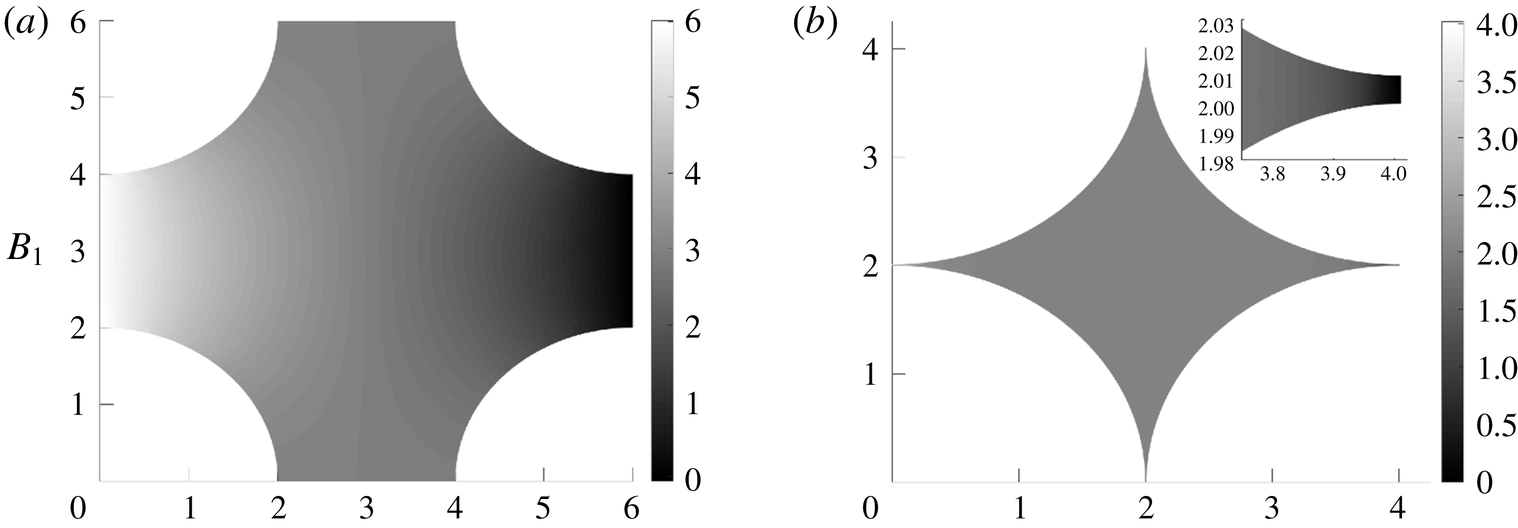
Heat maps plotting
 $B_{1}$
for two different unit-cell sizes are shown in figure 4. It is clear from these plots that the drop in
 $B_{1}$
across the unit cell is more gradual for
 $H=6.0a$
and occurs over a larger distance than the drop for
 $H=4.01a$
. This is to be expected from the lubrication analysis, according to which the length over which the drop occurs scales with
 $\unicode[STIX]{x1D716}^{1/2}$
.
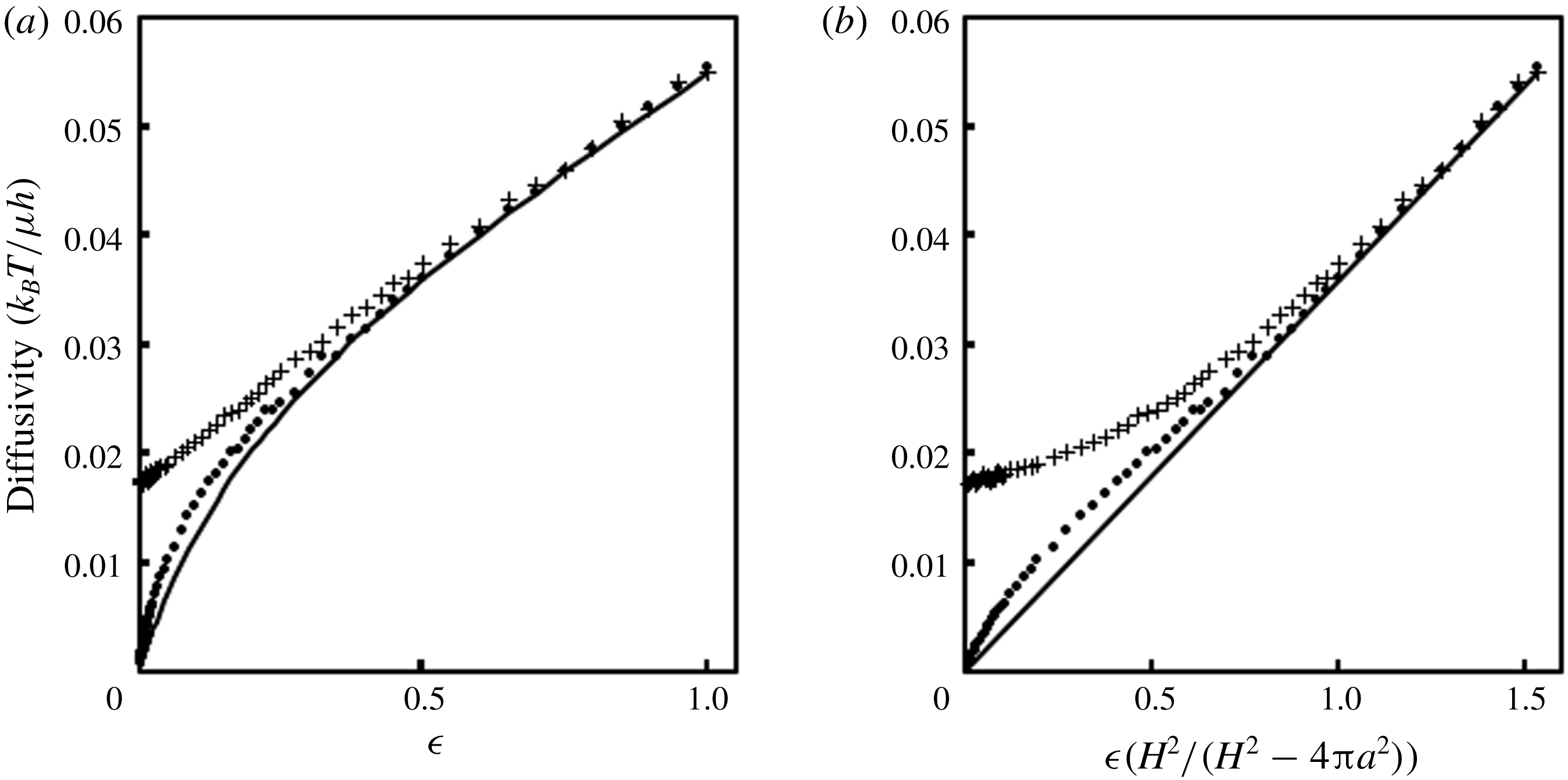
The
 $x_{1}$
-component of the long-time diffusivity due to a concentration gradient in
 $x_{1}$
,
 $D_{L}=D_{L11}$
, was found for different values of
 $H$
and is plotted versus
 $\unicode[STIX]{x1D716}$
in figure 5(a). For this problem,
 $D_{L11}$
is the only element of interest because
 $D_{L11}=D_{L22}$
due to symmetry and
 $D_{L12}=D_{L21}=0$
. The short-time diffusivity components
 $D_{s11}$
and
 $D_{s22}$
were also spatially averaged over the unit cell (denoted as
 $\langle D_{s}\rangle$
) and are plotted in figure 5(a). As expected,
 $\langle D_{s}\rangle$
remains non-zero even when
 $D_{L}$
reaches zero at
 $\unicode[STIX]{x1D716}=0$
. This is because there are still pore spaces between the immobilized particles which are accessible to the mobile particle. Even though these pore spaces are disconnected (and thus do not support long-time diffusivity), the mobile particle still has non-zero short-time diffusivity in them. The short-time diffusivities must be averaged according to (3.8) to give the proper long-time behaviour. The lubrication result derived in the previous section is also plotted in figure 5(a). The same results are plotted versus
 $H^{2}\unicode[STIX]{x1D716}/(H^{2}-4\unicode[STIX]{x03C0}a^{2})$
in figure 5(b) to facilitate better comparison between the FEM result and lubrication result, which is linear in this plot. There is good agreement between the lubrication and FEM results for
 $D_{L}$
. However, the FEM result is slightly larger than the lubrication result for smaller gap sizes. This may be because we have accounted for rotational couplings in our FEM calculations, but we have not done so in our lubrication calculation. Surprisingly, there is agreement between the FEM results for square arrays and the lubrication results even at large gap sizes.
Polynomial fits for
 $D_{s}$
and
 $D_{L}$
may be useful for experimentalists studying model systems. These fits are as follows:
 $$\begin{eqnarray}\displaystyle \left.\begin{array}{@{}c@{}}D_{s}=-0.0558\unicode[STIX]{x1D716}^{5}+0.1503\unicode[STIX]{x1D716}^{4}-0.144\unicode[STIX]{x1D716}^{3}+0.0535\unicode[STIX]{x1D716}^{2}+0.0341\unicode[STIX]{x1D716}+0.0173,\quad 0\leqslant \unicode[STIX]{x1D716}\leqslant 1,\\ D_{L}=0.7073\unicode[STIX]{x1D716}^{5}-1.9314\unicode[STIX]{x1D716}^{4}+1.9423\unicode[STIX]{x1D716}^{3}-0.8899\unicode[STIX]{x1D716}^{2}+0.2282\unicode[STIX]{x1D716},\quad 0\leqslant \unicode[STIX]{x1D716}\leqslant 1.\end{array}\right\} & & \displaystyle \nonumber\\ \displaystyle & & \displaystyle\end{eqnarray}$$
The agreement with the lubrication result gave us confidence that our FEM scheme accurately incorporated the interactions we desired. Therefore, we used our FEM to investigate diffusion through random arrays of immobile disks for different immobile area fractions,
 $\unicode[STIX]{x1D719}_{I}$
. Before examining those results, however, we introduce a network analysis for random arrays that makes use of our FEM and lubrication results and can be used to access larger system sizes.
Heat maps of
 $B_{1}$
plotted for the fluid region of one unit cell for square arrays of two different sizes: (a)
 $H=6.0a$
and (b)
 $H=4.01a$
. The horizontal and vertical axes show position within the unit cell. The shading of the fluid region represents the value of
 $B_{1}$
according to the adjacent scale bars.

Comparison of FEM results for square arrays with lubrication analysis. Plus signs are spatially averaged short-time diffusivities from computations. Solid circles are long-time diffusivities from our FEM implementation. The solid line is the long-time diffusivity computed from the lubrication analysis.

4 Network analysis in random arrays
While the FEM described above is accurate, it is too computationally expensive to access large system sizes, which are needed to capture the long tortuous paths by which mobile particles diffuse through random arrays with high immobile area fractions. To access larger system sizes, we made an abstraction of our diffusion model that will simplify computations considerably. In this abstraction, we use Voronoi tessellation to construct a network of pore spaces between immobilized proteins and employ a simple rule to determine the flow rate of mobile particles along the bonds of the network in the presence of a concentration gradient. This idea was briefly suggested in the context of transmembrane protein diffusion by Sung & Yethiraj (Reference Sung and Yethiraj2006), but similar approaches have been used to study pressure-driven flow in porous materials (Charlaix, Guyon & Roux Reference Charlaix, Guyon and Roux1987). In our model, a concentration drop equal to the unit-cell size
 $L$
is applied across a periodic unit cell of randomly arranged non-overlapping disks in a manner similar to our FEM approach. In our treatment here, we will apply the concentration gradient along the
 $x_{1}$
-direction and explain how to compute
 $D_{L11}$
, the component of the long-time diffusivity in
 $x_{1}$
due to a concentration gradient in
 $x_{1}$
. A similar treatment could be used to compute
 $D_{L22}$
.
A Voronoi tessellation gives a network of vertices and edges in which all edges are equidistant between two neighbouring immobile disks and all vertices are equidistant between three neighbouring immobile disks. The vertices can be interpreted as pore spaces between the immobile disks, and the edges can be interpreted as bonds between those pores. Each vertex is bonded to three other vertices. After Voronoi tessellation of the void space, a simple geometric criterion is applied to determine which bonds are open: if the centre-to-centre distance between the two immobile obstacles that share a given bond is greater than
 $4a$
, then the bond is considered to be open because a mobile disk can diffuse through the gap between the immobile disks. All other bonds are considered closed. After the bond connectivity is determined, the vertices that are part of a network of bonds which span the unit cell in
 $x_{1}$
are isolated and analysed. For these vertices, the flow rate of isolated mobile particles through a given bond can be related to the concentrations of the corresponding vertices as follows:
 $$\begin{eqnarray}\displaystyle Q_{mn}=-A(\unicode[STIX]{x1D716})\unicode[STIX]{x0394}B_{1}, & & \displaystyle\end{eqnarray}$$
where
 $$\begin{eqnarray}\displaystyle \unicode[STIX]{x0394}B_{1} & = & \displaystyle L+B_{1m}-B_{1n}~\text{for bonds crossing the unit-cell boundary in the }x_{1}\text{-direction},\nonumber\\ \displaystyle & = & \displaystyle B_{1m}-B_{1n}~\text{otherwise}.\end{eqnarray}$$
Here,
 $Q_{mn}$
is the flow rate of mobile disks to
 $m$
from
 $n$
between connected vertices
 $m$
and
 $n$
,
 $B_{1m}$
(
 $B_{1n}$
) is the concentration of mobile disks at vertex
 $m$
(
 $n$
), and
 $x_{1m}$
(
 $x_{1n}$
) is the
 $x_{1}$
-coordinate of the vertex
 $m$
(
 $n$
), with
 $x_{1m}\geqslant x_{1n}$
. The flow rate through a bond is the integral of the flux of mobile disks across the gap between two immobile disks corresponding to that bond. The coefficient
 $A(\unicode[STIX]{x1D716})$
relates the flow rate to the concentration drop and is a function of the half-gap
 $\unicode[STIX]{x1D716}$
(defined as in § 3.2) between the two immobile disks corresponding to the bond. We used FEM results for ordered arrays to calculate
 $A(\unicode[STIX]{x1D716})$
, described below. The first relation in (4.2) enforces the concentration drop across the unit cell by adding
 $L$
to the concentration difference for these bonds. Because the system is at steady state, the sum of flow rates through each vertex
 $m$
is zero:
 $$\begin{eqnarray}\displaystyle \mathop{\sum }_{n}Q_{mn}=0. & & \displaystyle\end{eqnarray}$$
Here, the summation is over all vertices
 $n$
that are bonded to
 $m$
. Using these relations, the concentrations at each vertex can be determined. After this is done, the flow rates for bonds that cross a unit-cell boundary can be added to determine an averaged flux. The concentration gradient averaged across the entire unit cell must be computed in a manner analogous to that of the lubrication problem. In particular, we have specified a concentration gradient which applies in the accessible part of the fluid phase only, and we must relate it to the gradient averaged across the entire unit cell:
 $$\begin{eqnarray}\displaystyle \left\langle \frac{\text{d}B_{1}}{\text{d}x_{1}}\right\rangle _{f}=\frac{L^{2}}{A_{f}}\left\langle \frac{\text{d}B_{1}}{\text{d}x_{1}}\right\rangle . & & \displaystyle\end{eqnarray}$$
Here, just as in (3.14),
 $\langle \text{d}B_{1}/\text{d}x_{1}\rangle _{f}$
is the gradient averaged over the fluid phase only, and
 $\langle \text{d}B_{1}/\text{d}x_{1}\rangle$
is the gradient averaged over the entire unit cell. We determine
 $A_{f}$
by sampling random points within the unit cell and determining whether any immobile particles are centred a distance less than or equal to
 $2a$
from them. The long-time diffusivity component
 $D_{L11}$
can then be computed from the familiar constitutive relation:
 $$\begin{eqnarray}\displaystyle \langle q\rangle =\frac{1}{L}\mathop{\sum }_{\langle m,n\rangle }Q_{mn}=D_{L11}\left\langle \frac{\text{d}B_{1}}{\text{d}x_{1}}\right\rangle =D_{L11}\frac{A_{f}}{L^{2}}, & & \displaystyle\end{eqnarray}$$
where the sum is over all bonds corresponding to vertex pairs
 $\langle m,n\rangle$
that cross a unit-cell boundary.
4.1 Determination of coefficient
 $A(\unicode[STIX]{x1D716})$
from FEM calculations

Because random arrays of disks have similar local structure and coordination number to hexagonal arrays, we felt that we may be able to estimate the coefficient
 $A(\unicode[STIX]{x1D716})$
in random arrays by approximating them as hexagonal arrays and systematically varying
 $\unicode[STIX]{x1D716}$
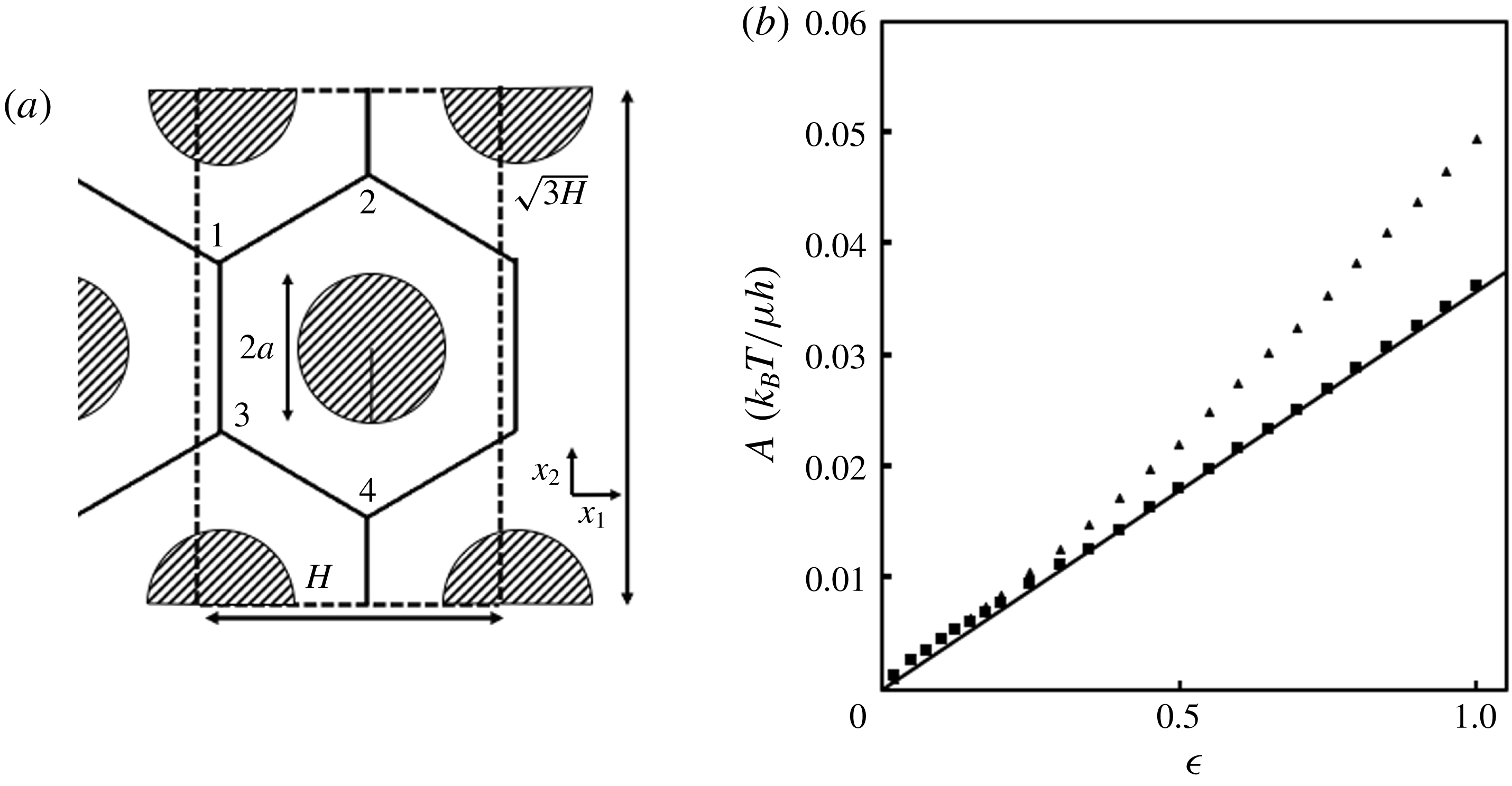
. This would allow us to conveniently use our FEM to find a simple relation which would be accurate for higher area fractions of randomly arranged immobilized disks. We therefore used our FEM to calculate long-time diffusivities of a mobile disk in hexagonal arrays of immobile disks as a function of the half-gap
 $\unicode[STIX]{x1D716}$
. Arrays of 24 immobile disks were used to compute short-time diffusivities, and a rectangular unit cell containing two immobile disks was used in FEM computations to calculate
 $D_{L}$
. This rectangular unit cell is shown in figure 6.
Computation of
 $A(\unicode[STIX]{x1D716})$
. (a) Hexagonal array of immobilized disks. The rectangular unit cell used for FEM computations is outlined in dashed lines. Vertices and edges corresponding to a Voronoi tessellation of the fluid space are shown as solid lines. The vertices of one particular unit cell are labelled 1–4. (b) Plot of
 $A$
as a function of
 $\unicode[STIX]{x1D716}$
. Solid triangles are FEM results from hexagonal arrays, solid squares are FEM results from square arrays, and the solid line is the lubrication result.

To compute the coefficient
 $A$
from these results, we had to determine the relationship between
 $A$
, relating a flow rate to a concentration drop, and
 $D_{L}$
, relating a flux to a concentration gradient. We did this by carrying out an analysis consistent with our network analysis (NA) on a hexagonal array. A Voronoi tessellation was carried out on the unit cell in figure 6, yielding four vertices. The NA above was then used to apply a concentration drop across the unit cell and calculate the resulting flow rate. If a concentration drop
 $H$
is applied along the
 $x_{1}$
-axis, the flow rate across the right boundary of the unit cell is
 $$\begin{eqnarray}\displaystyle Q_{hex}=A_{hex}H. & & \displaystyle\end{eqnarray}$$
In this case, all bonds have the same coefficient,
 $A_{hex}$
, because they are all the same width. This flow rate can be divided by the length of the right boundary to give the average flux of mobile particles:
 $$\begin{eqnarray}\displaystyle \langle q\rangle _{hex}=Q_{hex}/(\sqrt{3}H)=A_{hex}/\sqrt{3}. & & \displaystyle\end{eqnarray}$$
Now using (4.5), a diffusion coefficient can be calculated. In this case, the factor
 $A_{f}/L^{2}$
can be calculated analytically and is equal to
 $(\sqrt{3}H^{2}-8\unicode[STIX]{x03C0})/\sqrt{3}H^{2}$
. This gives
 $$\begin{eqnarray}\displaystyle \langle q\rangle _{hex}=D_{L,hex}\frac{\sqrt{3}H^{2}}{\sqrt{3}H^{2}-8\unicode[STIX]{x03C0}a^{2}}. & & \displaystyle\end{eqnarray}$$
Equating the previous two expressions gives the following relation between
 $A_{hex}$
and
 $D_{L,hex}$
:
 $$\begin{eqnarray}\displaystyle A_{hex}=D_{L,hex}\frac{3H^{2}}{\sqrt{3}H^{2}-8\unicode[STIX]{x03C0}a^{2}}. & & \displaystyle\end{eqnarray}$$
After calculating
 $D_{L,hex}$
for different half-gaps,
 $A_{hex}$
was calculated and is plotted in figure 6(b). For comparison, coefficients computed from the lubrication analysis and from FEM results on square arrays are also plotted. Because the lubrication problem for square arrays was posed as a flow rate induced by a concentration difference (in the same manner as the NA), the computation of
 $A$
from
 $D_{L}$
for it is straightforward. One must simply remove the extra factor accounting for the excluded volume of immobilized disks:
 $$\begin{eqnarray}\displaystyle A_{lub}=\frac{\unicode[STIX]{x1D716}}{\sqrt{2}\unicode[STIX]{x03C0}I_{3}}\frac{k_{b}T}{\unicode[STIX]{x1D707}h}. & & \displaystyle\end{eqnarray}$$
Here,
 $A_{lub}$
is the coefficient
 $A$
from the lubrication problem. This result applies to arrays of any geometry and could be adapted to compute
 $D_{L}$
for other periodic arrays. A similar procedure can be used to compute the coefficient,
 $A_{sq}$
, based on FEM results for square arrays:
 $$\begin{eqnarray}\displaystyle A_{sq}=D_{L,sq}\frac{H^{2}-4\unicode[STIX]{x03C0}a^{2}}{H^{2}}, & & \displaystyle\end{eqnarray}$$
where
 $D_{L,sq}$
is the long-time diffusivity from FEM on square arrays. Figure 6(b) shows that the result for hexagonal arrays at finite
 $\unicode[STIX]{x1D716}$
is significantly larger than the results from lubrication and square arrays. A polynomial fit to the results for hexagonal arrays up to
 $\unicode[STIX]{x1D716}=4$
, given below, was used as part of the NA on random arrays:
 $$\begin{eqnarray}\displaystyle A_{hex}=0.00058\unicode[STIX]{x1D716}^{4}-0.00612\unicode[STIX]{x1D716}^{3}+0.01813\unicode[STIX]{x1D716}^{2}+0.03713\unicode[STIX]{x1D716},\quad 0<\unicode[STIX]{x1D716}<4. & & \displaystyle\end{eqnarray}$$
5 Long-time diffusivity in random arrays
5.1 Comparison of finite element method and network analysis
FEM computations for the long-time diffusivity of one mobile protein in random arrays of immobile proteins were carried out on the small system sizes accessible with this rigorous method. Unit cells with
 $N_{I}=35$
randomly arranged non-overlapping disks were generated by randomly inserting the disks into the unit cell and carrying out Brownian dynamics simulations to move the disks from these positions. The size of the unit cell was calculated by specifying a particular immobile area fraction
 $\unicode[STIX]{x1D719}_{I}$
. The portion of the unit cell outside of the excluded-volume surface of the mobile protein was then meshed. A typical mesh contained approximately 100 000 nodes. After computing the short-time diffusivity for a mobile disk at each node within an FEM mesh in a random array, equation (3.1) was solved using the FEM previously described and (3.8) was used to compute the long-time diffusivity of the mobile disk in the array. For each immobile area fraction, the diagonal elements
 $D_{L11}$
and
 $D_{L22}$
were averaged for at least
 $50$
arrays and used to compute the scalar long-time diffusivity
 $D_{L}$
.
Random arrays introduce a potential complication into our FEM scheme: the fluid space accessible to the mobile particle is not completely connected in some random arrays. In some cases, portions of the fluid space were not spatially connected to all unit-cell boundaries, making it impossible to determine
 $\boldsymbol{B}$
at the nodes in those regions using the specified boundary conditions. We note, however, that
 $\unicode[STIX]{x1D735}\boldsymbol{B}$
must be zero in these closed regions, so they do not contribute to the computation of
 $\unicode[STIX]{x1D63F}_{\boldsymbol{L}}$
except in the trivial computation of
 $A_{f}$
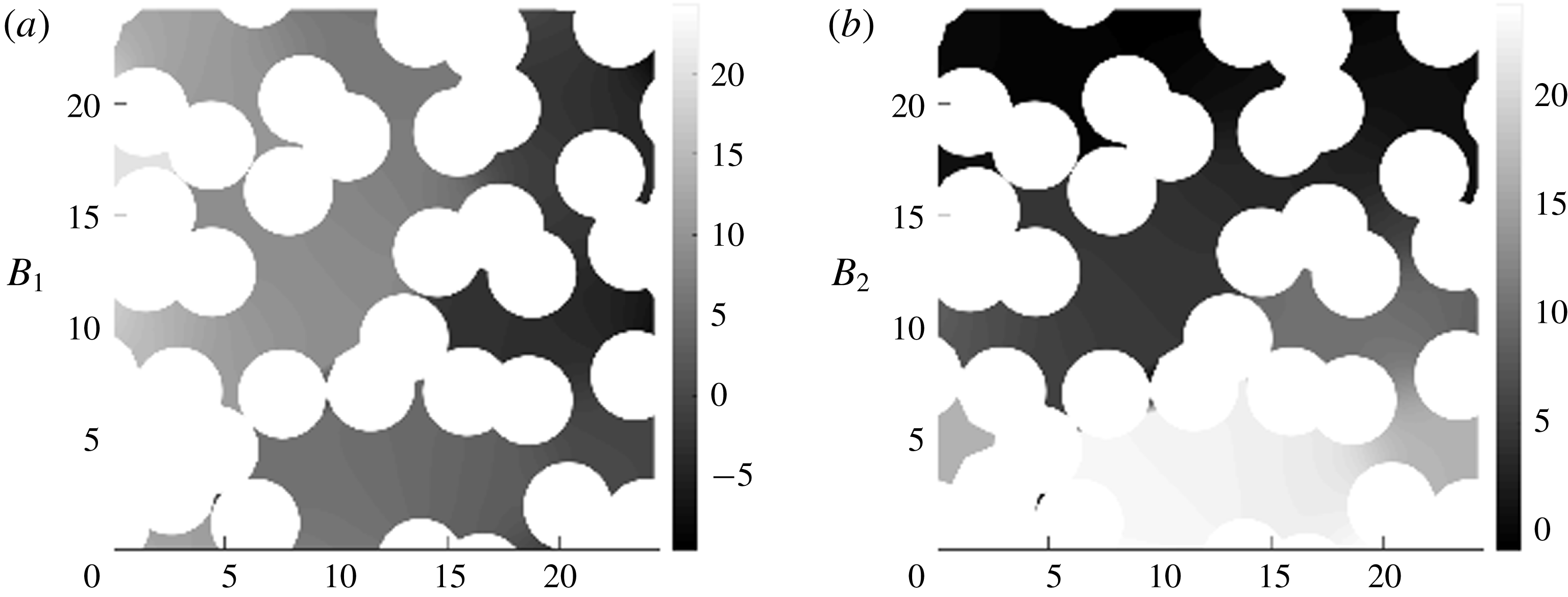
. Therefore, these disconnected fluid regions were treated in a manner similar to excluded-volume regions and were not included in the FEM computations. Sample heat maps depicting
 $B_{1}$
and
 $B_{2}$
for one particular random array are shown in figure 7. Marked changes in
 $B_{1}$
and
 $B_{2}$
can be seen across multiple small gaps in the array. These plots show the profound effect of small gaps on the concentration profile and the long-time diffusivity of the mobile disk.
Heat maps depicting
 $B_{1}$
and
 $B_{2}$
for one representative random array. One array of randomly arranged disks with
 $\unicode[STIX]{x1D719}_{I}=0.16$
and
 $N_{I}=30$
is shown. The circular occlusions represent both the immobile disks and the excluded area of the mobile disk around them. Values for (a)
 $B_{1}$
and (b)
 $B_{2}$
are depicted by the shading of the regions of the unit cell accessible to the mobile particle according to the adjacent scale bars.

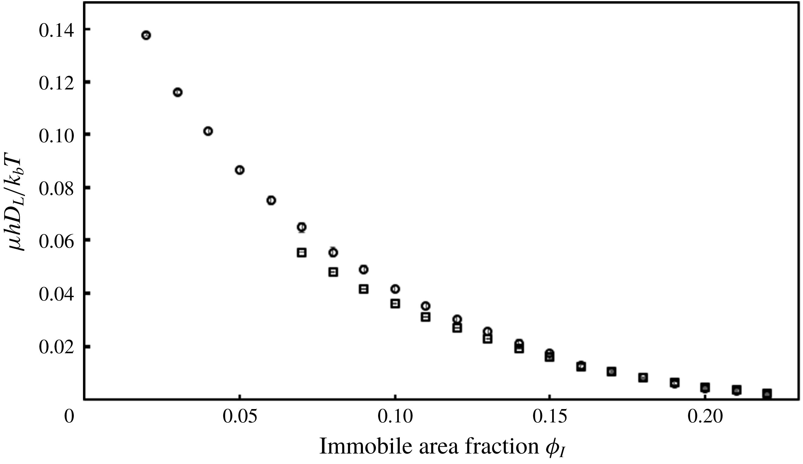
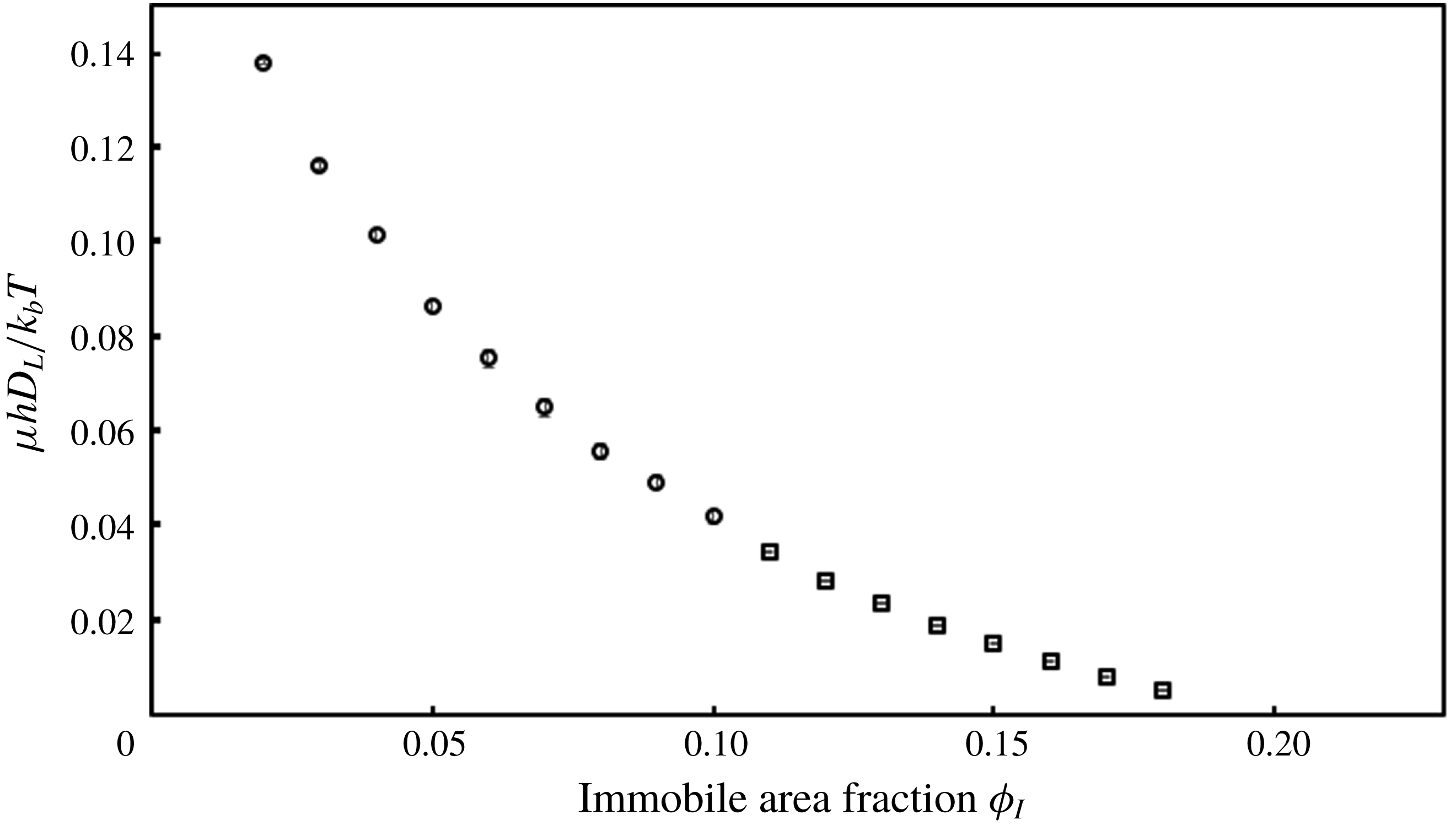
Long-time diffusivity versus immobile area fraction for random arrays with
 $N_{I}=35$
. Open circles are from the FEM. Open squares are from the NA. Standard errors with 95 % confidence intervals are shown.

Figure 8 shows
 $D_{L}$
computed from FEM as a function of
 $\unicode[STIX]{x1D719}_{I}$
. As one would expect, the long-time diffusivity decreases as the immobile area fraction increases. For comparison, for
 $\unicode[STIX]{x1D706}=250$
, which is believed to be a typical value for a lipid bilayer, equation (1.1) gives
 $D_{0}\approx 0.39k_{b}T/\unicode[STIX]{x1D707}h$
. The marked decrease seen in figure 8 is due to a combination of hydrodynamic and thermodynamic effects from the immobile disks. However, finite-size effects can be seen close to the percolation threshold at
 $\unicode[STIX]{x1D719}_{I}\approx 0.22$
. At this immobile area fraction, the long-time diffusivity through an infinitely large random array would be
 $0$
. The small array sizes in these calculations do not account for the long tortuous paths taken by a mobile particle in an infinite array and thus give higher long-time diffusivities than in larger arrays.
Using the NA to determine the size dependence of
 $D_{L}$
at different immobile area fractions, we found that finite-size effects on the long-time diffusivity are seen at
 $N_{I}=35$
for
 $\unicode[STIX]{x1D719}_{I}>0.10$
. We used the NA to provide accurate results at larger system sizes by first comparing the results from the two methods for
 $N_{I}=35$
. This allowed us to use the more accurate FEM results to calculate a correction to the results from the NA to account for the local resistance of the pores. The computations for the NA were carried out on the same random arrays as those generated for the rigorous FEM computations. Again,
 $D_{L11}$
and
 $D_{L22}$
were averaged to compute the scalar long-time diffusivity
 $D_{L}$
. These long-time diffusivities are plotted alongside the FEM results in figure 8. For the results shown, the maximum percentage difference between the two methods is approximately 15 % at
 $\unicode[STIX]{x1D719}_{I}=0.07$
. This is not surprising because the NA does not accurately account for resistance to the particle motion within pore spaces and would therefore become less accurate for larger pore spaces.
We used the FEM results to calculate a correction to the NA results. Such a correction would ostensibly allow us to scale up to larger system sizes while still accurately representing the hydrodynamic interactions in the membrane. The ratio of the FEM result to the NA result for each immobile area fraction was fitted to a polynomial function. The polynomial function obtained is
 $$\begin{eqnarray}\displaystyle g(\unicode[STIX]{x1D719}_{I})=78.204\unicode[STIX]{x1D719}_{I}^{3}-44.562\unicode[STIX]{x1D719}_{I}^{2}+5.674\unicode[STIX]{x1D719}_{I}+0.9569,\quad 0.07\leqslant \unicode[STIX]{x1D719}_{I}\leqslant 0.22. & & \displaystyle\end{eqnarray}$$
For the results obtained by the NA that follow, the scalar long-time diffusivity computed in the manner described above was multiplied by this correction factor to obtain more accurate results:
 $$\begin{eqnarray}\displaystyle D_{L}=g(\unicode[STIX]{x1D719}_{I})D_{L,NA}. & & \displaystyle\end{eqnarray}$$
Here,
 $D_{L,NA}$
is the long-time diffusivity obtained from the NA by averaging
 $D_{L11}$
and
 $D_{L22}$
for random arrays of immobile proteins.
5.2 Extension to infinitely large arrays
Using the NA with the hydrodynamic correction above, we attempted to compute long-time diffusivities for a mobile protein in infinitely large random arrays of immobile proteins. We did so by calculating long-time diffusivities at different system sizes with fixed
 $\unicode[STIX]{x1D719}_{I}$
. The diffusivities were calculated from random arrays generated in the manner previously described. For each
 $\unicode[STIX]{x1D719}_{I}$
and each
 $N_{I}$
, at least
 $200$
arrays were generated. For
 $\unicode[STIX]{x1D719}_{I}\leqslant 0.10$
, we found that the long-time diffusivity did not change appreciably with system size above
 $N_{I}=35$
. We thus concluded that our FEM results for
 $N_{I}=35$
accurately represented the long-time diffusivity in infinitely large arrays at those immobile area fractions. For
 $\unicode[STIX]{x1D719}_{I}>0.10$
, we calculated the long-time diffusivity using the NA for increasing system sizes until the long-time diffusivity stopped changing. These results are plotted in figure 9.
Estimate of long-time diffusivity versus immobile area fraction for infinitely large random arrays. Open circles indicate that the results were obtained from the FEM. Open squares indicate that the results are from the approximate method. Standard errors with 95 % confidence intervals are shown.

An empirical polynomial fit to these data may be of use to scientists who wish to compare experimental data to our model. It is given as follows:
 $$\begin{eqnarray}\displaystyle D_{L} & = & \displaystyle -2459.3\unicode[STIX]{x1D719}_{I}^{5}+1460.3\unicode[STIX]{x1D719}_{I}^{4}-344.22\unicode[STIX]{x1D719}_{I}^{3}+43.466\unicode[STIX]{x1D719}_{I}^{2}-3.6681\unicode[STIX]{x1D719}_{I}+0.1963,\quad \nonumber\\ \displaystyle & & \displaystyle \qquad 0.02\leqslant \unicode[STIX]{x1D719}_{I}\leqslant 0.18.\end{eqnarray}$$
We emphasize again here that this fit is strictly empirical and does not agree with the asymptotic limits given by Brinkman theory for small
 $\unicode[STIX]{x1D719}_{I}$
or by percolation theory near
 $\unicode[STIX]{x1D719}_{I}=\unicode[STIX]{x1D719}_{I,c}$
(discussed below), respectively.
As
 $\unicode[STIX]{x1D719}_{I}$
increases, the system sizes required to accurately compute the long-time diffusivity in an infinite array increases dramatically. This is illustrated in figure 10, which plots
 $D_{L}$
versus the number of immobilized disks,
 $N_{I}$
, for a few immobile area fractions. For larger area fractions, we increased values of
 $N_{I}$
in factors of
 $2^{1/2}$
until the computed long-time diffusivity changed less than 1 % from the value for the previous system size twice. The maximum immobile area fraction for which we calculated the long-time diffusivity was
 $\unicode[STIX]{x1D719}_{I}=0.18$
. This required us to access arrays with
 $N_{I}=2^{13}=8192$
. Similar calculations at
 $\unicode[STIX]{x1D719}_{I}=0.19$
and
 $\unicode[STIX]{x1D719}_{I}=0.20$
continued to show system size dependence up to
 $N_{I}=8192$
. The difficulty in computing the long-time diffusivity for these higher values of
 $\unicode[STIX]{x1D719}_{I}$
led us to consider alternatives to the methods we developed. Sung & Yethiraj (Reference Sung and Yethiraj2006, Reference Sung and Yethiraj2008) characterized a critical immobile area fraction,
 $\unicode[STIX]{x1D719}_{I,c}\approx 0.22$
, at which long-range transport of a mobile protein ceases and the long-time diffusivity becomes zero. Their work suggests that we can treat
 $\unicode[STIX]{x1D719}_{I,c}$
as a percolation threshold and use percolation theory to study the diffusive properties near
 $\unicode[STIX]{x1D719}_{I,c}$
. Percolation theory provides simple scaling laws for properties such as diffusivity near the percolation threshold. We explored the applicability of this theory to this system by comparing finite-size scaling results to the relevant scaling law from percolation theory.
Long-time diffusivity versus number of immobilized proteins
 $N_{I}$
for the indicated immobile area fractions. Standard errors with 95 % confidence intervals are shown.

Finite-size scaling of
 $D_{L}/$
with respect to system size at
 $\unicode[STIX]{x1D719}_{I}=0.21$
. Open circles indicate that the results were obtained from the FEM. Open squares indicate that the results are from the NA. The solid black line and the dashed line are linear fits to the FEM data and the NA data, respectively, with fixed slope
 $=-0.975$
. Standard errors with 95 % confidence intervals are shown.

Effect of hydrodynamic interactions on the ratio of long-time to short-time diffusivity. (a) The ratio
 $D_{L}/\langle D_{s}\rangle$
is plotted versus gap size for square arrays of immobile particles. The solid line is the lubrication result without hydrodynamics, the open circles are FEM results without hydrodynamics, the solid squares are lubrication results with hydrodynamics, and the solid circles are FEM results with hydrodynamics. (b) Plot of
 $D_{L}/\langle D_{s}\rangle$
versus immobile area fraction for random arrays. Solid circles show FEM results with hydrodynamic interactions, and open circles show FEM results without hydrodynamic interactions. The solid line is dilute theory. Standard errors with 95 % confidence intervals are shown.

6 Finite-size scaling near percolation threshold
To study the long-time diffusivity at higher immobile area fractions, we investigated the possibility of using percolation theory to interpret our results for unit-cell sizes that were too small to provide an accurate direct estimate of
 $D_{L}$
. Sung & Yethiraj (Reference Sung and Yethiraj2006, Reference Sung and Yethiraj2008) carried out Voronoi tessellations of random arrays of immobile circular disks and analysed the resulting network of bonds between the void spaces of the disks to determine whether the network could support transport of mobile disks. These authors identified a percolation threshold at a critical immobile area fraction,
 $\unicode[STIX]{x1D719}_{I,c}\approx 0.22$
, above which long-range transport is not supported. Their work suggests that our results for
 $(\unicode[STIX]{x1D719}_{I,c}-\unicode[STIX]{x1D719}_{I})/\unicode[STIX]{x1D719}_{I,c}\ll 1$
can be interpreted using percolation theory.
Many quantities that characterize a system exhibit power-law scaling at or near the percolation threshold (Stauffer & Aharony Reference Stauffer and Aharony1994). A correlation length,
 $\unicode[STIX]{x1D709}$
, characterizes the size of clusters of obstacles to diffusion. When the system size,
 $L$
, is much smaller than
 $\unicode[STIX]{x1D709}$
, the long-time diffusivity exhibits power-law scaling with system size at fixed
 $\unicode[STIX]{x1D719}_{I}$
:
 $$\begin{eqnarray}\displaystyle D_{L}=kL^{-\unicode[STIX]{x1D702}/\unicode[STIX]{x1D708}},\quad L\ll \unicode[STIX]{x1D709}. & & \displaystyle\end{eqnarray}$$
Here,
 $\unicode[STIX]{x1D702}$
and
 $\unicode[STIX]{x1D708}$
are universal scaling exponents. In two dimensions,
 $\unicode[STIX]{x1D702}\approx 1.3$
and
 $\unicode[STIX]{x1D708}=4/3$
. To test the validity of this relation, we examined the finite-size scaling of our diffusivity results at
 $\unicode[STIX]{x1D719}_{I}=0.21$
. We computed long-time diffusivities for different system sizes using the NA method. We also carried out FEM computations for system sizes accessible with that method. For each unit-cell size, diffusivities were computed from between
 $200$
and
 $400$
random arrangements. The results are plotted on a log–log scale in figure 11. Linear fits with fixed slope of
 $-\unicode[STIX]{x1D702}/\unicode[STIX]{x1D708}\approx -0.975$
are shown for both sets of data. Our datasets show agreement with the prediction from percolation theory, indicating that percolation theory may provide an adequate framework to analyse long-time diffusion for values of
 $\unicode[STIX]{x1D719}_{I}$
for which we cannot access the long-time diffusivity using the NA method. According to the fits, the coefficient in (6.1) is
 $k=0.0712$
for the FEM calculations and
 $k=0.0683$
for the NA calculations.
7 Hydrodynamic effects on
$D_{L}/\langle D_{s}\rangle$

Finally, to gain insight into the nature of hydrodynamic interactions (HIs) in this problem and to compare our results for
 $D_{L}$
in random arrays with those of Bussell et al. (Reference Bussell, Koch and Hammer1995) and Dodd et al. (Reference Dodd, Hammer, Sangani and Koch1995), we examined the effect of hydrodynamics on the ratio
 $D_{L}/\langle D_{s}\rangle$
. Bussell et al. (Reference Bussell, Koch and Hammer1995) and Dodd et al. (Reference Dodd, Hammer, Sangani and Koch1995) assumed that HIs do not change this ratio in order to obtain their results. Figure 12 shows plots of
 $D_{L}/\langle D_{s}\rangle$
as a function of gap size for square arrays (figure 12
a) and as a function of immobile area fraction for random arrays (figure 12
b).
In figure 12(a), for FEM results with HIs, spatially averaged short-time diffusivities,
 $\langle D_{s}\rangle$
, were calculated for a given unit cell by choosing random points within the fluid portion of each of the arrays, computing the short-time diffusivity for a mobile disk placed at these points, and averaging over the diagonal elements,
 $D_{s11}$
and
 $D_{s22}$
, of each short-time diffusivity. The long-time diffusivities were then divided by these spatially averaged short-time diffusivities to give the ratio plotted in the figure. The lubrication result for
 $D_{L}$
given by (3.23) was also divided by
 $\langle D_{s}\rangle$
to obtain an expression for
 $D_{L}/\langle D_{s}\rangle$
by lubrication analysis. For FEM results without HIs, the ratio was computed for the same square unit cells by setting the short-time diffusivity at each node in the mesh equal to the identity tensor and proceeding with the FEM calculation. For square arrays, the same approach was used in the lubrication analysis to give the following analytical estimate of the ratio in the absence of HIs:
 $$\begin{eqnarray}\displaystyle \frac{D_{L}}{\langle D_{s}\rangle }=\unicode[STIX]{x1D716}^{1/2}/\unicode[STIX]{x03C0}=\left(\frac{1}{2}\left(\sqrt{\frac{\unicode[STIX]{x03C0}}{\unicode[STIX]{x1D719}_{I}}}-2\right)\right)^{1/2}/\unicode[STIX]{x03C0}. & & \displaystyle\end{eqnarray}$$
Corresponding results for random arrays are shown in figure 12(b). For this case, in the dilute limit
 $\unicode[STIX]{x1D719}_{I}\ll 1$
, an analysis similar to Maxwell’s calculation of the effective conductivity of a composite suspension can be used to obtain an estimate of the ratio which is valid without HIs (Zimmerman, Chen & Cook Reference Zimmerman, Chen and Cook1992):
 $$\begin{eqnarray}\displaystyle \frac{D_{L}}{\langle D_{s}\rangle }=1-4\unicode[STIX]{x1D719}_{I}. & & \displaystyle\end{eqnarray}$$
This expression is also plotted in figure 12(b) as a solid line. The FEM result without HIs agrees with the dilute theory for small
 $\unicode[STIX]{x1D719}_{I}$
but becomes significantly lower than the result from dilute theory at larger
 $\unicode[STIX]{x1D719}_{I}$
as the structure of the immobile obstacles makes the possible diffusion pathways of the mobile disk more tortuous.
Interestingly, for both square and random arrays, the ratio
 $D_{L}/\langle D_{s}\rangle$
with HIs is significantly higher than the result without HIs. This suggests that the HIs between the immobile disks and the mobile one affect the manner in which the thermodynamic interactions between the immobile disks and the mobile one manifest in these systems. Therefore, it is inappropriate to treat hydrodynamic and thermodynamic interactions separately and later combine their effects to estimate the long-time diffusivity in these colloidal systems, as done by Bussell et al. (Reference Bussell, Koch and Hammer1995) and Dodd et al. (Reference Dodd, Hammer, Sangani and Koch1995). This result differs significantly from the corresponding result in three 3-D all-mobile colloidal suspensions. In such systems, Brady (Reference Brady1994) presented rigorous arguments to show that the long-time diffusivity could be computed by considering only hydrodynamic effects on
 $\langle D_{s}\rangle$
and only thermodynamic effects on
 $D_{L}/\langle D_{s}\rangle$
and multiplying these results together. Others have applied this approach to 3-D suspensions with immobile occlusions and have shown agreement with experimental results for diffusion of macromolecules in agarose gels (Johnson et al.
Reference Johnson, Berk, Jain and Deen1996; Phillips Reference Phillips2000). However, we do not know of any rigorous arguments put forth for this factorization between hydrodynamic and thermodynamic effects in partially immobile suspensions.
Our results thus show that hydrodynamic effects on the long-time diffusivity in partially immobile 2-D colloidal suspensions differ markedly from those in all-mobile 3-D suspensions. This difference would ostensibly be due to either the stronger HIs in 2-D suspensions or the presence of immobile particles (or both). Bussell et al. (Reference Bussell, Hammer and Koch1994) computed the short-time diffusivity and the long-time diffusivity of proteins in all-mobile cell membranes and showed that HIs decrease the effect of hard-core thermodynamic interactions in slowing the long-time diffusivity of the mobile disks. This result is qualitatively similar to the result we have found in partially immobile cell membranes here and suggests that the difference between the system we have treated and an all-mobile 3-D colloidal suspension arises from the stronger HIs seen in 2-D suspensions (or quasi-2-D suspensions in the case of the system treated by Bussell et al. (Reference Bussell, Hammer and Koch1994)).
8 Conclusion
We have determined the long-time diffusivity of a single mobile transmembrane protein in cell membranes with randomly arranged immobile transmembrane proteins. Treating the proteins as cylinders embedded within a thin viscous fluid, we computed the hydrodynamic and thermodynamic effects of the immobilized cylinders on the diffusion of the mobile cylinder. As expected, the long-time diffusivity decreases with the area fraction of immobile proteins,
 $\unicode[STIX]{x1D719}_{I}$
. According to our analysis, long-time diffusion appears to be arrested near
 $\unicode[STIX]{x1D719}_{I}=0.22$
, consistent with previous analyses of random arrays which do not account for hydrodynamics. Our methods limit us to one mobile protein and prevent us from examining the effect of other mobile proteins on the long-time diffusivity of a mobile protein. Because it has been shown that the presence of immobile proteins reduces the short-time diffusivity much more than the presence of similar fractions of mobile proteins (Dodd et al.
Reference Dodd, Hammer, Sangani and Koch1995), we believe that our results apply in real cell membranes which contain multiple mobile proteins.
These results required the deployment of several complementary methods. We used a rigorous multipole expansion method to compute the short-time diffusivity of a mobile protein at an arbitrary location in a square unit cell with arbitrarily arranged immobile proteins. We then used these short-time diffusivities as part of an FEM to compute the long-time diffusivity in square arrays of immobile proteins as a function of the gap distance between the immobile proteins. After describing a lubrication analysis for the long-time diffusivity in square arrays valid at small gap distances, and showing agreement between results from our FEM and the lubrication analysis, we proceeded to develop an approximate NA which allowed us to access larger arrays of immobile proteins. We used the FEM and NA to estimate the long-time diffusivity of a mobile protein in an infinite array of immobile proteins. We were able to access system sizes large enough to obtain long-time diffusivities for immobile area fractions as large as
 $\unicode[STIX]{x1D719}_{I}=0.18$
. Finally, we showed that finite-size scaling of the long-time diffusivity close to the percolation threshold at
 $\unicode[STIX]{x1D719}_{I,c}\approx 0.22$
agrees with the prediction from percolation theory.
Empirical polynomial fits to our results for diffusivities in square and random arrays were provided for those who may find them convenient for comparison. We summarize them again here.
 $$\begin{eqnarray}\displaystyle \left.\begin{array}{@{}l@{}}\text{Square arrays:}\\ D_{s}=-0.0558\unicode[STIX]{x1D716}^{5}+0.1503\unicode[STIX]{x1D716}^{4}-0.144\unicode[STIX]{x1D716}^{3}+0.0535\unicode[STIX]{x1D716}^{2}+0.0341\unicode[STIX]{x1D716}+0.0173,\quad 0\leqslant \unicode[STIX]{x1D716}\leqslant 1,\\ D_{L}=0.7073\unicode[STIX]{x1D716}^{5}-1.9314\unicode[STIX]{x1D716}^{4}+1.9423\unicode[STIX]{x1D716}^{3}-0.8899\unicode[STIX]{x1D716}^{2}+0.2282\unicode[STIX]{x1D716},\quad 0\leqslant \unicode[STIX]{x1D716}\leqslant 1.\\ \text{Random arrays:}\\ D_{L}=-2459.3\unicode[STIX]{x1D719}_{I}^{5}+1460.3\unicode[STIX]{x1D719}_{I}^{4}-344.22\unicode[STIX]{x1D719}_{I}^{3}+43.466\unicode[STIX]{x1D719}_{I}^{2}-3.6681\unicode[STIX]{x1D719}_{I}+0.1963,\\ \quad 0.02\leqslant \unicode[STIX]{x1D719}_{I}\leqslant 0.18.\end{array}\right\} & & \displaystyle \nonumber\\ \displaystyle & & \displaystyle\end{eqnarray}$$
This work has interesting physical implications. Remarkably, the ratio of the long-time diffusivity to the short-time diffusivity,
 $D_{L}/\langle D_{s}\rangle$
, is larger with our hydrodynamic model than in the absence of hydrodynamic interactions. This is different from the behaviour found in all-mobile 3-D suspensions (Brady Reference Brady1994). Our work points to an interesting interplay between hydrodynamic and thermodynamic interactions that may make it impossible to decouple the two interactions in transmembrane protein diffusion. This interplay may result from the strength of the hydrodynamic interactions in two dimensions. Our result suggests that other work which has attempted to treat hydrodynamic and thermodynamic interactions separately (Bussell et al.
Reference Bussell, Koch and Hammer1995; Dodd et al.
Reference Dodd, Hammer, Sangani and Koch1995) may not accurately capture their combined effect on transmembrane protein diffusion. Nevertheless, our work reinforces an important result from that previous work: the profound effect that hydrodynamic interactions with immobilized proteins play in slowing the diffusion of mobile transmembrane proteins. Our results show that biologically relevant concentrations (
 $\unicode[STIX]{x1D719}_{I}\approx 0.10$
) of immobile proteins could slow the long-time diffusivity of a mobile protein by up to an order of magnitude. Hydrodynamic effects account for much more of this drop than excluded-volume effects.
The work described here can be extended in a number of directions to more accurately capture the properties of real cell membranes. For example, one could examine heterogeneities in the distribution of immobile proteins. Such heterogeneities appear to be important in diffusive phenomena such as hop diffusion (Fujiwara et al.
Reference Fujiwara, Ritchie, Murakoshi, Jacobson and Kusumi2002). In addition, the effect of mobile proteins on other mobile proteins could be examined using dynamic simulation. The modification we have introduced to compute short-time diffusivity tensors which are symmetric would allow us to use this method in dynamic simulations in a manner similar to simulation methods for 3-D colloidal suspensions (Ermak & McCammon Reference Ermak and McCammon1978; Brady & Bossis Reference Brady and Bossis1988; Grassia, Hinch & Nitsche Reference Grassia, Hinch and Nitsche1995; Banchio & Brady Reference Banchio and Brady2003). These simulation methods would also allow us to include more exotic thermodynamic interactions than the simple hard-core interactions investigated here. Finally, the agreement of our finite-size scaling results with percolation theory opens the possibility to use percolation theory to explore other aspects of diffusion in random arrays near
 $\unicode[STIX]{x1D719}_{I,c}$
. Near the percolation threshold, it is known that subdiffusive behaviour is seen on length scales much smaller than the correlation length which characterizes the structure of immobile proteins. This behaviour transitions to diffusive behaviour on length scales larger than the correlation length. The cross-over time is the approximate time at which the diffusive mode switches from subdiffusive to diffusive. Our methods would allow us to estimate cross-over times as a function of
 $\unicode[STIX]{x1D719}_{I}$
. This would be valuable in light of the numerous experimental reports of anomalous diffusion in cell membranes and model membrane platforms (Schütz et al.
Reference Schütz, Schindler and Schmidt1997; Ratto & Longo Reference Ratto and Longo2003; Przybylo et al.
Reference Przybylo, Skora, Humpolíková, Benda, Zan and Hof2006; Skaug, Faller & Longo Reference Skaug, Faller and Longo2011; Weigel et al.
Reference Weigel, Simon, Tamkun and Krapf2011).
Acknowledgements
The authors gratefully acknowledge support from NSF grant CBET 1803156 to D.L.K.; NSF grants CBET 1149452 and CMMI 1728049 and the R. F. Smith School Innovation Fund to S.D.; and an NSF GK-12 Grass-Roots Fellowship (DGE-1045513) to R.R.S.
Appendix A
Section 2 briefly explains the method of Dodd et al. (Reference Dodd, Hammer, Sangani and Koch1995) to compute short-time diffusivities for random arrangements of circular disks in a periodic unit cell by multipole expansion. We give more details here.
The Green’s functions
 $S_{1}$
and
 $S_{2}$
are related to each other by
 $$\begin{eqnarray}\displaystyle \unicode[STIX]{x1D6FB}^{2}S_{2}=S_{1}, & & \displaystyle\end{eqnarray}$$
where
 $S_{1}$
satisfies the relation
 $$\begin{eqnarray}\displaystyle \unicode[STIX]{x1D6FB}^{2}S_{1}(\boldsymbol{x})=4\unicode[STIX]{x03C0}\left(\frac{1}{L^{2}}-\mathop{\sum }_{\boldsymbol{r}_{0,n}}\unicode[STIX]{x1D6FF}(\boldsymbol{x}-\boldsymbol{r}_{0,n})\right), & & \displaystyle\end{eqnarray}$$
in which
 $\boldsymbol{r}_{0,n}$
are the lattice vectors.
When the coefficients
 $A_{nm}^{(s)}$
and
 $B_{nm}^{(s)}$
given in (2.4)–(2.6) correspond to the disk
 $n$
around which integration takes place in (2.3) (when
 $s=n$
), the terms from those coefficients are singular. The fluid velocity can be split into a singular part and a regular part:
 $$\begin{eqnarray}\displaystyle \boldsymbol{u}=\boldsymbol{u}_{\boldsymbol{s}}+\boldsymbol{u}_{\boldsymbol{r}}. & & \displaystyle\end{eqnarray}$$
The integrals in (2.3) can be carried out for the regular contribution
 $\boldsymbol{u}_{\boldsymbol{r}}$
using the following formulae from Sangani & Yao (Reference Sangani and Yao1988):
 $$\begin{eqnarray}\displaystyle & & \displaystyle \frac{1}{2\unicode[STIX]{x03C0}}\int _{0}^{2\unicode[STIX]{x03C0}}\boldsymbol{u}_{\boldsymbol{ r}}(\boldsymbol{x})\cos l\unicode[STIX]{x1D703}\,\text{d}\unicode[STIX]{x1D703}\nonumber\\ \displaystyle & & \displaystyle \quad =\frac{1}{2}(1+\unicode[STIX]{x1D6FF}_{l0})\frac{a^{l}}{l!}\left[\left(\frac{\unicode[STIX]{x2202}}{\unicode[STIX]{x2202}x_{1}}\right)^{l}-\frac{l}{4}\left(\frac{\unicode[STIX]{x2202}}{\unicode[STIX]{x2202}x_{1}}\right)^{(l-2)}\unicode[STIX]{x1D6FB}^{2}+\frac{a^{2}}{4(1+l)}\left(\frac{\unicode[STIX]{x2202}}{\unicode[STIX]{x2202}x_{1}}\right)^{l}\unicode[STIX]{x1D6FB}^{2}\right]\boldsymbol{u}_{\boldsymbol{r}}(\boldsymbol{x}^{(n)}),\nonumber\\ \displaystyle & & \displaystyle\end{eqnarray}$$
 $$\begin{eqnarray}\displaystyle & & \displaystyle \frac{1}{2\unicode[STIX]{x03C0}}\int _{0}^{2\unicode[STIX]{x03C0}}\boldsymbol{u}_{\boldsymbol{ r}}(\boldsymbol{x})\sin l\unicode[STIX]{x1D703}\,\text{d}\unicode[STIX]{x1D703}\nonumber\\ \displaystyle & & \displaystyle \quad =\frac{1}{2}\frac{a^{l}}{l!}\left[\left(\frac{\unicode[STIX]{x2202}}{\unicode[STIX]{x2202}x_{1}}\right)^{l-1}\left(\frac{\unicode[STIX]{x2202}}{\unicode[STIX]{x2202}x_{2}}\right)-\frac{l-2}{4}\left(\frac{\unicode[STIX]{x2202}}{\unicode[STIX]{x2202}x_{1}}\right)^{(l-3)}\left(\frac{\unicode[STIX]{x2202}}{\unicode[STIX]{x2202}x_{2}}\right)\unicode[STIX]{x1D6FB}^{2}\right.\nonumber\\ \displaystyle & & \displaystyle \qquad +\left.\frac{a^{2}}{4(1+l)}\left(\frac{\unicode[STIX]{x2202}}{\unicode[STIX]{x2202}x_{1}}\right)^{l-1}\left(\frac{\unicode[STIX]{x2202}}{\unicode[STIX]{x2202}x_{2}}\right)\unicode[STIX]{x1D6FB}^{2}\right]\boldsymbol{u}_{\boldsymbol{r}}(\boldsymbol{x}^{(n)}).\end{eqnarray}$$
Here the integration is assumed to be around the surface of a disk centred at
 $\boldsymbol{x}=\boldsymbol{x}^{(n)}$
. The singular terms must be integrated separately.
The mean velocity components
 $U_{1}$
and
 $U_{2}$
depend on whether all of the disks are mobile. When all of the disks are mobile, the forces applied to the disks are balanced by a pressure drop across the unit cell, and
 $U_{1}$
and
 $U_{2}$
are defined to be zero. In applications to reconstituted membranes, the mean velocity is then determined by the renormalization and matching to the outer solution discussed in Dodd et al. (Reference Dodd, Hammer, Sangani and Koch1995). When some of the disks are immobile, there is no pressure drop across the cell and the net force on all of the disks must be zero. In this case,
 $U_{1}$
and
 $U_{2}$
are unknowns and must be found by including two extra equations in addition to the boundary conditions: the sum of the forces in the
 $x_{1}$
- and the
 $x_{2}$
-direction must be zero.
A.1 Derivatives of
$S_{1}$
and
$S_{2}$


To carry out the method above, one must calculate the derivatives of
 $S_{1}$
and
 $S_{2}$
with respect to
 $x_{1}$
and
 $x_{2}$
. We briefly describe two methods for calculating these derivatives. These are similar to previous treatments by Sangani & Behl (Reference Sangani and Behl1989) and Sangani, Zhang & Prosperetti (Reference Sangani, Zhang and Prosperetti1991). Because all derivatives of
 $S_{1}$
satisfy the Laplace equation, all derivatives
 $\unicode[STIX]{x2202}_{1}^{p}\unicode[STIX]{x2202}_{2}^{q}S_{1}=(\unicode[STIX]{x2202}^{p+q}/\unicode[STIX]{x2202}x_{1}^{\,p}\unicode[STIX]{x2202}x_{2}^{q})S_{1}$
and
 $\unicode[STIX]{x2202}_{1}^{p}\unicode[STIX]{x2202}_{2}^{q}S_{2}=(\unicode[STIX]{x2202}^{p+q}/\unicode[STIX]{x2202}x_{1}^{\,p}\unicode[STIX]{x2202}x_{2}^{q})S_{2}$
can easily be calculated from the derivatives for which
 $q=0$
or
 $1$
. Therefore, we only describe the method to calculate derivatives for which
 $p=n$
and
 $q=0$
or
 $p=n-1$
and
 $q=1$
.
A.1.1 Ewald summation
The method of Ewald is fast and accurate for lower orders of differentiation
 $n=p+q$
. We use it for
 $n\leqslant 6$
. The expression for
 $S_{1}$
and
 $S_{2}$
can be written as follows (Hasimoto Reference Hasimoto1959):
 $$\begin{eqnarray}\displaystyle S_{m}(\boldsymbol{x}) & = & \displaystyle \frac{1}{\unicode[STIX]{x03C0}\unicode[STIX]{x1D70F}}\left(-\frac{1}{4\unicode[STIX]{x03C0}^{2}}\right)^{m-1}\frac{\unicode[STIX]{x03C0}^{m}\unicode[STIX]{x1D6FC}^{m}}{(m-1)!}\left[\unicode[STIX]{x1D70F}\unicode[STIX]{x1D6FC}^{-1}\mathop{\sum }_{n}\unicode[STIX]{x1D719}_{-m}\left(\frac{\unicode[STIX]{x03C0}r_{n}^{2}}{\unicode[STIX]{x1D6FC}}\right)-\frac{1}{m}\right.\nonumber\\ \displaystyle & & \displaystyle +\left.\mathop{\sum }_{\boldsymbol{k}\neq \mathbf{0}}\exp (2\unicode[STIX]{x03C0}\text{i}\boldsymbol{k}\boldsymbol{\cdot }\boldsymbol{x})\unicode[STIX]{x1D719}_{m-1}(\unicode[STIX]{x03C0}\unicode[STIX]{x1D6FC}k^{2})\right],\quad m=1,2.\end{eqnarray}$$
Here,
 $\unicode[STIX]{x1D70F}$
is the area of the unit cell (equal to
 $L^{2}$
in our case),
 $\unicode[STIX]{x1D6FC}$
is a constant, which we take to be equal to
 $\unicode[STIX]{x1D70F}$
,
 $r_{n}^{2}=|\boldsymbol{x}-\boldsymbol{r}_{0,n}|^{2}$
,
 $\boldsymbol{k}$
are the reciprocal lattice vectors, and
 $\unicode[STIX]{x1D719}_{\unicode[STIX]{x1D708}}(z)$
is the incomplete gamma function, defined as
 $$\begin{eqnarray}\displaystyle \unicode[STIX]{x1D719}_{\unicode[STIX]{x1D708}}(z)=\int _{1}^{\infty }\unicode[STIX]{x1D709}^{\unicode[STIX]{x1D708}}\exp (-z\unicode[STIX]{x1D709})\,\text{d}\unicode[STIX]{x1D709}. & & \displaystyle\end{eqnarray}$$
It is helpful to define other differential operators:
 $$\begin{eqnarray}\displaystyle \left.\begin{array}{@{}l@{}}\unicode[STIX]{x1D709}=x_{1}+\text{i}x_{2},\quad \unicode[STIX]{x1D702}=x_{1}-\text{i}x_{2},\\ \unicode[STIX]{x1D6E5}_{m}=\unicode[STIX]{x2202}_{\unicode[STIX]{x1D709}}^{m}+\unicode[STIX]{x2202}_{\unicode[STIX]{x1D702}}^{m}\quad \text{for}~m>0,\\ \phantom{\unicode[STIX]{x1D6E5}_{m}}=1\quad \text{for}~m=0,\\ \phantom{\unicode[STIX]{x1D6E5}_{m}}=0\quad \text{for}~m<0,\\ \tilde{\unicode[STIX]{x1D6E5}}_{m}=\text{i}(\unicode[STIX]{x2202}_{\unicode[STIX]{x1D709}}^{m}-\unicode[STIX]{x2202}_{\unicode[STIX]{x1D702}}^{m})\quad \text{for}~m>0,\\ \phantom{\tilde{\unicode[STIX]{x1D6E5}}_{m}}=0\quad \text{for}~m\leqslant 0.\end{array}\right\} & & \displaystyle\end{eqnarray}$$
Now we have
 $$\begin{eqnarray}\displaystyle \left.\begin{array}{@{}c@{}}\displaystyle \unicode[STIX]{x2202}_{1}^{n}S_{1}=\unicode[STIX]{x0394}S_{1}+\frac{n}{4}\frac{4\unicode[STIX]{x03C0}}{\unicode[STIX]{x1D70F}}\unicode[STIX]{x1D6FF}_{n2},\quad n\geqslant 0,\\ \displaystyle \unicode[STIX]{x2202}_{1}^{n}S_{2}=\unicode[STIX]{x0394}S_{2}+\frac{n}{4}\unicode[STIX]{x1D6E5}_{n-2}S_{1}+\frac{n(n-1)}{32}\frac{4\unicode[STIX]{x03C0}}{\unicode[STIX]{x1D70F}}\unicode[STIX]{x1D6FF}_{n4},\quad n\geqslant 0,\\ \displaystyle \unicode[STIX]{x2202}_{1}^{n-1}\unicode[STIX]{x2202}_{2}S_{1}=\tilde{\unicode[STIX]{x0394}}S_{1},\quad n>0,\\ \displaystyle \unicode[STIX]{x2202}_{1}^{n-1}\unicode[STIX]{x2202}_{2}S_{2}=\tilde{\unicode[STIX]{x0394}}S_{2}+\frac{n-2}{4}\tilde{\unicode[STIX]{x1D6E5}}_{n-2}S_{1},\quad n>0.\end{array}\right\} & & \displaystyle\end{eqnarray}$$
Now the differentiation can be split into regular and singular contributions:
 $$\begin{eqnarray}\displaystyle \left.\begin{array}{@{}c@{}}\unicode[STIX]{x1D6E5}_{n}S_{m}=\unicode[STIX]{x1D6E5}_{n}S_{m}^{reg}+\unicode[STIX]{x1D6E5}_{n}S_{m}^{sing},\\ \tilde{\unicode[STIX]{x1D6E5}}_{n}S_{m}=\tilde{\unicode[STIX]{x1D6E5}}_{n}S_{m}^{reg}+\tilde{\unicode[STIX]{x1D6E5}}_{n}S_{m}^{sing}.\end{array}\right\} & & \displaystyle\end{eqnarray}$$
The regular contributions are

The singular contributions are
 $$\begin{eqnarray}\displaystyle \left.\begin{array}{@{}l@{}}\displaystyle \unicode[STIX]{x1D6E5}_{n}S_{1}^{sing}=-2\ln r\quad \text{for}~n=0,\\ \displaystyle =2(n-1)!(-1)^{n}r^{-n}\cos (n\unicode[STIX]{x1D703})\quad \text{for}~n\geqslant 0,\\ \displaystyle \tilde{\unicode[STIX]{x1D6E5}}_{n}S_{1}^{sing}=2(n-1)!(-1)^{n}r^{-n}\sin (n\unicode[STIX]{x1D703})\quad \text{for}~n\geqslant 0,\\ \displaystyle \unicode[STIX]{x1D6E5}_{n}S_{2}^{sing}={\textstyle \frac{1}{2}}r^{2}(1-\ln r)\quad \text{for}~n=0,\\ \displaystyle =2r~\cos \unicode[STIX]{x1D703}\left({\textstyle \frac{1}{4}}-{\textstyle \frac{1}{2}}\ln r\right)\quad \text{for}~n=1,\\ \displaystyle ={\textstyle \frac{1}{2}}r^{-n+2}\cos n\unicode[STIX]{x1D703}\quad (n-2)!(-1)^{n+1}~\text{for}~n\geqslant 2,\\ \displaystyle \tilde{\unicode[STIX]{x1D6E5}}_{n}S_{2}^{sing}=2r\sin \unicode[STIX]{x1D703}\left({\textstyle \frac{1}{4}}-{\textstyle \frac{1}{2}}\ln r\right)\quad \text{for}~n=1,\\ \displaystyle ={\textstyle \frac{1}{2}}r^{-n+2}\sin n\unicode[STIX]{x1D703}(n-2)!(-1)^{n+1}\quad \text{for}~n\geqslant 2.\end{array}\right\} & & \displaystyle\end{eqnarray}$$
Substituting the expressions in (A 11) and (A 12) into (A 10) and then into (A 9) allows one to find the derivatives of
 $S_{1}$
and
 $S_{2}$
.
A.1.2 Direct summation
A direct lattice sum can be employed for higher orders of differentiation using the following expressions:
 $$\begin{eqnarray}\displaystyle & \displaystyle \unicode[STIX]{x2202}_{1}^{p}\unicode[STIX]{x2202}_{2}^{q}S_{1}(\boldsymbol{r})=-2\mathop{\sum }_{\boldsymbol{r}_{0,n}}\unicode[STIX]{x2202}_{1}^{p}\unicode[STIX]{x2202}_{2}^{q}\ln s,\quad n=p+q>2, & \displaystyle\end{eqnarray}$$
 $$\begin{eqnarray}\displaystyle & \displaystyle \unicode[STIX]{x2202}_{1}^{p}\unicode[STIX]{x2202}_{2}^{q}S_{2}(\boldsymbol{r})=-\frac{1}{2}\mathop{\sum }_{\boldsymbol{r}_{0,n}}\unicode[STIX]{x2202}_{1}^{p}\unicode[STIX]{x2202}_{2}^{q}s^{2}\ln s,\quad n=p+q>4, & \displaystyle\end{eqnarray}$$
where
 $s=|\boldsymbol{r}-\boldsymbol{r}_{0,n}|$
. Singular contributions must be added separately as described in the previous section.