The cluster-robust standard error (CRSE) first proposed by Liang and Zeger (Reference Liang and Zeger1986) has become ubiquitous in applied quantitative work in political science since it was implemented in Stata by Rogers (Reference Rogers1993). The reasons for its ubiquity are straightforward: the problems that clustered data present for statistical analysis are well-known to political scientists (Moulton Reference Moulton1986, Reference Moulton1990), and CRSEs are extremely simple to estimate and useful when added to a research design involving fixed effects estimation (Bertrand, Duflo and Mullainathan Reference Bertrand, Duflo and Mullainathan2004). But it is not as widely understood that using CRSEs without regard to their limitations can produce very misleading inferences. Research has shown that CRSE confidence intervals are too narrow and false positive ratesFootnote 1 are substantially in excess of the nominal size of a statistical hypothesis test when the number of clusters in a data set is small (Cameron, Gelbach and Miller Reference Cameron, Gelbach and Miller2008; Green and Vavreck Reference Green and Vavreck2008; Angrist and Pischke Reference Angrist and Pischke2009, Chapter 8; Harden Reference Harden2011). There is no universal cutoff for how many clusters is “small;” prior research tends to put the threshold of elevated concern somewhere around 40 clusters, although this threshold can be much higher in some circumstances (MacKinnon and Webb Reference MacKinnon and Webb2017). Nevertheless, we find that political scientists are still very likely to employ CRSEs in this situation. We speculate that CRSEs are still used in data sets with few clusters because (a) no alternatives are as easy to implement in Stata and R, and (b) the limitations of CRSEs are not sufficiently publicized in political science.
Our paper makes two contributions to the political science literature. Our primary contribution is to make it easy for substantive researchers to use alternatives to the CRSE as a normal part of their workflow. Toward this end, we create and make available pre-packaged routines for estimating cluster-adjusted t-statistics (CATs) (Ibragimov and Müller Reference Ibragimov and Müller2010), pairs cluster bootstrapped t-statistics (PCBSTs) (Bertrand, Duflo and Mullainathan Reference Bertrand, Duflo and Mullainathan2004; Cameron, Gelbach and Miller Reference Cameron, Gelbach and Miller2008; Harden Reference Harden2011), and wild cluster bootstrapped t-statistics (WCBSTs) (Cameron, Gelbach and Miller Reference Cameron, Gelbach and Miller2008) for common models. These routines are in the clusterSEs package for R and the clustse and clusterbs ado files for Stata.Footnote 2
We also explain why these alternatives perform better than CRSEs in data sets with a small number of clusters and provide simulation evidence in favor of this argument. In our simulations, we find that CATs are usually more effective (and always at least as effective) at limiting false positives compared with CRSEs, PCBSTs, and WCBSTs. CATs are also often more powerful at detecting true positives (rejections of the null hypothesis when the null is false) compared with alternatives. Although CATs cannot be estimated in any cluster with unidentified coefficients (e.g., without variation on the dependent variable), we provide both an analytic argument and simulation evidence that simply dropping these clusters allows CATs to be effectively used. Finally, although random effects (RE) models have better size and power characteristics in our simulation compared with any cluster adjustment alternative when the model is correctly specified, cluster adjustments do substantially better when the assumptions of the RE model are not satisfied.
To substantively illustrate how CRSEs can be misleading in data sets with few clusters, we re-examine three recently published analyses by Grosser, Reuben and Tymula (Reference Grosser, Reuben and Tymula2013), Lacina (Reference Lacina2014), and Hainmueller, Hiscox and Sequeira (Reference Hainmueller, Hiscox and Sequeira2015) using alternative approaches. Grosser, Reuben and Tymula (Reference Grosser, Reuben and Tymula2013) observed that candidates for office in an experiment lower their proposals for redistribution in response to increased donations from a rich voter; our reanalysis with CATs finds that this relationship is more uncertain than shown by the original CRSE-based analysis (and in some cases is statistically insignificant). In Lacina (Reference Lacina2014), we find little evidence in the replication data set for a link between political representation and civil unrest in India when using PCBSTs; this is contrary to Lacina’s original conclusion derived using CRSEs. Our reanalysis of the evidence in Hainmueller, Hiscox and Sequeira (Reference Hainmueller, Hiscox and Sequeira2015) generally supports the authors’ conclusion that consumers are willing to pay more for products with a “fair trade” label; however, we find that there is substantially more uncertainty in the magnitude of this relationship using CATs or PCBSTs than the original analysis using CRSEs would indicate.
THE ANALYSIS OF CLUSTERED DATA: PROBLEMS AND SOLUTIONS
Data in political science are frequently grouped; as one example, survey observations of individual respondents are often clustered by geographical units (counties, states, countries, etc.). We expect that respondents inside of a cluster are related to one another in complex ways that may be difficult to understand or model. For statistical analysis, this poses the difficulty that the random component of observed outcomes cannot be treated as independently and identically distributed within a cluster. Accounting for this statistical dependence between observations is a well-known problem in the statistical literature. In data sets where the data exhibits some dependency between observations in the same cluster, ignoring this dependence can greatly underestimate the true standard errors (SEs) for parameters of interest when this clustering structure is associated with the independent variable (Moulton Reference Moulton1986; Moulton Reference Moulton1990). This can lead to researchers falsely rejecting the null hypothesis of a statistical significance test too frequently, resulting in an excess of published papers with conclusions that are not supported by the data.
There are many approaches to dealing with clustered structure in a data set of interest. When a fixed effects model is desired (e.g., as a part of a difference-in-difference research design), it is common to correct the SEs for residual cluster dependency (Bertrand, Duflo and Mullainathan Reference Bertrand, Duflo and Mullainathan2004). In this scenario, researchers commonly employ the cluster option in Stata (developed by Rogers Reference Rogers1993). This procedure is a modification of White’s (Reference White1980) robust SEs, altering the White “sandwich estimator” to allow for dependence between observations inside a cluster. CRSEs were described in the context of generalized estimating equations by Liang and Zeger (Reference Liang and Zeger1986), and were implemented in Stata by Rogers (Reference Rogers1993) (see also Arellano Reference Arellano1987). The formula for the cluster-robust variance-covariance matrix in ordinary least squares (OLS) regression is (Cameron and Miller Reference Cameron and Miller2015, 8–9):
 $$\:{\rm var}\,\:\hat{\beta }\,{\equals}\,\left( {X^{'} X} \right)^{\!{{\minus}1}} \left[ {\mathop{\sum}\limits_{g{\equals}1}^G \left[ {X_{g}^{'} \hat{u}_{g} \hat{u}_{g}^{'} X_{g} } \right]} \right](X^{'} X)^{{{\minus}1}} ,$$
where
 $$\hat{\beta }$$
are OLS estimates, G the number of clusters, X the N×m matrix of independent variables (for N observations and m variables), and
 $$\hat{u}_{g} $$
the vector of residuals
 $$y_{g} {\minus}X_{g} \hat{\beta }$$
in cluster g. Theorem 2 in Liang and Zeger (Reference Liang and Zeger1986, 16) demonstrates that, for models with intra-cluster error dependence but inter-cluster independence, the maximum likelihood estimator of
 $$\hat{\beta }$$
is consistent and multivariate Gaussian as G → ∞; the covariance of this distribution is consistently estimated by Equation 1 as G → ∞. The result also holds (with suitable adjustment of Equation 1) for other generalized linear model (GLM) models.
Following the introduction of CRSE to social science research, a series of papers have emphasized their ability to obtain accurate measures of uncertainty (and appropriately sized statistical significance tests) in a wide variety of scenarios (Liang and Zeger Reference Liang and Zeger1993; Donner Reference Donner1998; Williams Reference Williams2000; Klar and Donner Reference Klar and Donner2001; Kezdi Reference Kezdi2004; Bertrand, Duflo and Mullainathan Reference Bertrand, Duflo and Mullainathan2004). Of course, CRSEs are not a cure-all. Differences between the typical maximum likelihood SEs and CRSEs can indicate harmful misspecification problems that are not addressed by adjusting the variance-covariance matrix (Hardin and Hilbe Reference Hardin and Hilbe2003, 33–34). In these cases, CRSEs might be useful as a check on the appropriateness of the model’s specification (King and Roberts Reference King and Roberts2014). CRSEs can also be useful in cases where explicitly modeling some aspect of the data-generating process is problematic but a simplified model is still consistent (see e.g., Cameron and Trivedi Reference Cameron and Trivedi2005, 147–150). For example, Bertrand, Duflo and Mullainathan (Reference Bertrand, Duflo and Mullainathan2004) report that parametrically modeling residual serial correlation results in excess false positive rates for placebo treatments in a Monte Carlo analysis of Current Population Survey data and simulated data; CRSEs are more effective at limiting false positives in their study.Footnote 3
Unfortunately, evidence reveals a major problem with using CRSEs in data sets that have a small number of clusters: using CRSEs when the number of clusters is small can cause models to find statistically significant relationships where no relationships actually exist. That is, when only a small number of clusters are used in an analysis with clustered SEs, the CRSEs are biased downward (Mancl and DeRouen Reference Mancl and DeRouen2001; Donald and Lang Reference Donald and Lang2007; Cameron, Gelbach and Miller Reference Cameron, Gelbach and Miller2008; Angrist and Pischke Reference Angrist and Pischke2009; Ibragimov and Müller Reference Ibragimov and Müller2010; Imbens and Kolesar Reference Imbens and Kolesar2012). The CRSE procedure depends on an asymptotic justification that the number of clusters G (and not the number of observations per cluster) approaches infinity (Hansen Reference Hansen2007; Cameron, Gelbach and Miller Reference Cameron, Gelbach and Miller2008). This can be seen in Equation 1, where the center summation happens over the number of clusters G and not over the number of observations N; as a result, the accuracy and stability of the estimate relies on having access to many clusters, not many observations, because consistency of the center summation depends on G → ∞ (Cameron and Miller Reference Cameron and Miller2015, 7–9). Intuitively, if one has a data set with N many observations in G many clusters but is unwilling to assume that observations in different clusters are identically distributed, one is (in a sense) estimating SEs based on G many items of information. Consequently, any asymptotically derived results for the distribution of
 $$\hat{\beta }$$
will not apply unless G is very large, and significance tests or confidence intervals based on these asymptotically derived distributions will be inaccurate when G is small.
There is no hard-and-fast rule for how few clusters is too few for using CRSEs. The work of Cameron, Gelbach and Miller (Reference Cameron, Gelbach and Miller2008), Angrist and Pischke (Reference Angrist and Pischke2009), and Harden (Reference Harden2011) suggests that data sets with fewer than about 40 clusters are at substantively elevated risk of having downward-biased CRSEs. However, this threshold can vary under different circumstances; for example, simulations by MacKinnon and Webb (Reference MacKinnon and Webb2017) indicate that CRSEs can be problematic with as many as 100 clusters if the clusters have very different numbers of observations.
HOW OFTEN ARE CRSES USED WITH FEW CLUSTERS IN POLITICAL SCIENCE?
How often do political scientists use CRSEs in data sets with few clusters in published quantitative work? To answer this question, we gathered data from four highly visible general interest political science journals: American Political Science Review (APSR), American Journal of Political Science (AJPS), Journal of Politics (JOP), and International Studies Quarterly (ISQ) (hereafter known by their initials). We examined the use of CRSEs in every published article starting with the most recent issue (as of July 2014) and going back four years; we only go back four years to account for the fact that many of the articles highlighting the undesirable small-sample properties of CRSEs were published in the mid-to-late-2000s. For each article, we recorded the subfield, whether CRSEs were used, the number of clusters, and the number of observations. In the case of multiple models per article, we recorded the article that used the fewest clusters.
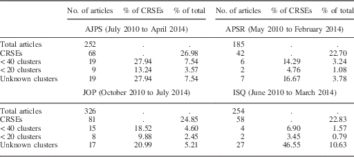
Table 1 displays the summary statistics for each journal. Between 20 and 27 percent of articles in each journal used CRSEs, with AJPS showing the highest prevalence. This journal also displayed the highest rate of models with fewer than 40 clusters (7.54 percent of all articles and 27.94 percent of articles that used clustering). AJPS also had a substantial proportion of papers with fewer than 20 clusters, representing 13.24 percent of all articles that used CRSEs. APSR and JOP fare somewhat better, with between 3 and 5 percent of all articles using clustering in data sets with fewer than 40 clusters (between 14 and 19 percent of all articles that used CRSEs). ISQ showed the lowest rate of articles with fewer than 40 clusters at 1.57 percent (6.90 percent of CRSE articles), but this journal showed the highest rate of models with an unknown number of clusters at 10.63 percent (46.55 percent of articles using CRSEs).
Use of Cluster-Robust Standard Errors (CRSE) in General Interest Journals in Political Science (2010–2014)

AJPS=American Journal of Political Science; APSR=American Political Science Review; JOP=Journal of Politics; ISQ=International Studies Quarterly.
WHAT ALTERNATIVES TO CRSES ARE AVAILABLE?
According to the prior literature on the subject, using CRSEs in a data set with a small number of clusters is ill-advised. We focus on three alternatives for cluster adjustment that are relatively versatile and simple. These options are as follows:
1. PCBSTs, variants of which are studied by Bertrand, Duflo and Mullainathan (Reference Bertrand, Duflo and Mullainathan2004), Cameron, Gelbach and Miller (Reference Cameron, Gelbach and Miller2008), and Harden (Reference Harden2011).
2. WCBSTs, as proposed by Cameron, Gelbach and Miller (Reference Cameron, Gelbach and Miller2008).
3. CATs, based on the work of Ibragimov and Müller (Reference Ibragimov and Müller2010) and also studied by Canay, Romano and Shaikh (Reference Canay, Romano and Shaikh2014).
Our primary contribution is the creation of a streamlined statistical package for implementing these alternative uncertainty estimators.Footnote 4 The replication materials for this paper include code for all these procedures for GLM and multinomial logit models in Stata and R; the code is available at the Comprehensive R Archive Network repository for R (under library name clusterSEs) and the Statistical Software Components archive repository for Stata (under the names clustse and clusterbs).Footnote 5 We describe the principles behind each procedure in the main body of the text, providing technically detailed step-by-step procedures for each one in an Online Appendix.
After describing these potential options and how their performance in data sets with a small number of clusters may differ,Footnote 6 we conduct a Monte Carlo analysis to evaluate their performance in relation to CRSEs and the usual maximum likelihood SEs (which we refer to hereafter as “vanilla” SEs). We also compare these techniques to a standard RE model (Wooldridge Reference Wooldridge2002, 257–265); this allows us to compare the performance of cluster adjustment techniques to that of a potentially more efficient model that is also potentially more sensitive to violations of its assumptions (Clark and Linzer Reference Clark and Linzer2015).
PCBSTs
The PCBST is a variation on the typical bootstrap procedure that accounts for the clustered structure of data. A typical bootstrapping process draws a bootstrap data set of size N with replacement from the original data set (also of size N), estimates the model of interest on the bootstrap data set, saves a quantity of interest (such as
 $$\hat{\beta }$$
) from this model, repeats the process K times for a large value of K, and then examines the empirical distribution of K-many values of
 $$\hat{\beta }_{k} $$
, k=1 … K. The bootstrap distribution of
 $$\hat{\beta }_{k} $$
will approximate the distribution of
 $$\hat{\beta }$$
(Efron Reference Efron1979; van der Vaart Reference van der Vaart1998, Chapters 19 and 23). If the bootstrapped quantity is
 $$\hat{\beta }$$
, its SEs can be estimated by the SEs of the replicates; alternatively, a 95 percent confidence interval can be estimated using the 2.5th and 97.5th quantiles of
 $$\hat{\beta }_{k} $$
.
The PCBST modifies this procedure (1) to sample clusters with replacement, rather than individual observations with replacement, and (2) to sample the test statistic
 $$t\,{\equals}\,\hat{\beta }/\hat{\sigma }$$
instead of
 $$\hat{\beta }$$
. The first modification to the usual bootstrap procedure is necessary to recognize that observations within a cluster are not independently distributed and thus we cannot resample at the level of the individual observation and still preserve the distribution of
 $$\hat{\beta }$$
. The second modification is used because t is pivotal (its large-sample distribution does not depend on the unknown true values of β and
 $$\sigma _{{\hat{\beta }}} $$
) and therefore its performance in small samples can in some cases be better than that for bootstrapping of non-pivotal statistics such as
 $$\hat{\beta }$$
(Liu and Singh Reference Liu and Singh1987; Horowitz Reference Horowitz1997). For calculating 95 percent confidence intervals, the 95th percentile value of t
z
may be used as a part of the normal formula for confidence intervals,
 $$\hat{\beta }\,\pm\,\left( {t_{{1{\minus}\alpha }} } \right)\hat{\sigma }$$
.
Thus, PCBSTs treat clusters rather than observations as the fundamental unit of analysis and implement the bootstrap at this level. Based on a Monte Carlo analysis, Harden recommends that “state politics researchers use [the pairs cluster bootstrap] to conduct statistical inference with clustered data” (Reference Harden2011, 224).Footnote 7 Bertrand, Duflo and Mullainathan (Reference Bertrand, Duflo and Mullainathan2004) study and apply PCBSTs (which they call the “block bootstrap”) and find that they are effective in controlling the size of hypothesis tests with serially correlated panel data for a moderate number of clusters in a difference-in-difference design, but produce excess false positives for a small number of clusters. However, they use vanilla SEs rather than CRSEs for the bootstrap replicates; Cameron, Gelbach and Miller (Reference Cameron, Gelbach and Miller2008) shows that CRSE replicates perform better with a small number of clusters.
WCBSTs
WCBSTs are similar to PCBSTs, but are based on the idea of “wild bootstrapping” the residuals of a regression rather than bootstrapping observations directly (Wu Reference Wu1986). The wild cluster bootstrap procedure relies on construction of error terms
 $$\hat{{\epsilon}}$$
from the original linear model
 $$y\,{\equals}\,X\hat{\beta }{\plus}\hat{{\varepsilon}}$$
, then creating new bootstrap data sets by sampling on clusters and assigning new values of the error term equal to the original estimated error term multiplied by weights randomly selected from a set, such as the two-point Rademacher weights {1, −1} (Liu Reference Liu1988).Footnote
8
As with any bootstrapping technique, the procedure relies on approximating the distribution of
 $$\hat{\beta }$$
using repeated resampling of the data and re-estimation of the model on the resampled data. But for WCBSTs, the model’s estimated error terms are treated as the source of variation in the observations. Cameron, Gelbach and Miller conclude that “this [wild cluster] bootstrap works well in our own simulation exercise and when applied to the data of Bertrand, Duflo and Mullainathan (Reference Bertrand, Duflo and Mullainathan2004)” (Reference Cameron, Gelbach and Miller2008, 425). Note that this procedure depends on estimates of the residuals
 $$\hat{{\varepsilon}}$$
, and is therefore unsuited for GLM models with non-standard residuals (e.g., the probit).Footnote
9
CATs
CATs were first suggested as an approach to modeling clustered data by Ibragimov and Müller (Reference Ibragimov and Müller2010). Intuitively, the contribution of Ibragimov and Müller (Reference Ibragimov and Müller2010) (and the proofs in Bakirov and Szekely (Reference Bakirov and Szekely2006) that underlie their work) is in determining the small-sample properties for an estimator that accounts for intra-cluster dependence among observations. This allows us to improve on the performance of CRSEs in a small number of clusters, wherein the performance of the CRSE estimator is analytically unknown.
The key theoretical insight for CATs (as described in Ibragimov and Müller (Reference Ibragimov and Müller2010, 455–456), which we repeat here) comes in realizing that, when the number of observations N
g
in every cluster g is large and cluster level estimates
 $$\hat{\beta }_{g} $$
are (asymptotically) independent, then for many common statistical estimators each cluster estimate
 $$\hat{\beta }_{g} $$
should take an asymptotic distribution (as N
g
→∞) of:
 $$\sqrt {N_{g} } \left( {\hat{\beta }_{g} {\minus}\,\beta } \right)\mathop{\,\sim\,}\limits^{{asym}} \Phi \left( {0,\sigma _{g}^{2} } \right).$$
This property flows from the well-known asymptotic properties of many estimators, including and especially the OLS regression estimator and maximum likelihood estimator for GLM–family models. Consequently, the vector of group-specific estimates
 $$\hat{\beta }_{{\bf G}} $$
takes the asymptotic distribution (as N
g
→∞ for all g∈{1, … , G}):
 $$\sqrt N \left( {\hat{\beta }_{{\bf G}} {\minus}\,\beta } \right)\mathop{\,\sim\,}\limits^{{asym}} \Phi ({\bf 0}, {\rm ∑}\nolimits_{\rm{G}} {} ) ,$$
with
 $$N\,{\equals}\,\mathop{\sum}\nolimits_{g{\equals}1}^G {N_{g} } ,\hat{\beta }_{{\bf G}} ^{T} {\equals}\left[ {\matrix{ {\hat{\beta }_{1} } & \!\!\!\!\!{...}\!\!\!\!\! & {\hat{\beta }_{G} } \cr } } \right]$$
and
 $$\mathop{\sum}\nolimits_{\bf{G}} {} \,{\equals}\,{\rm diag}\left( {\sigma _{{\rm 1}} ,...,\sigma _{G} } \right)$$
; the block-diagonal nature of
 $$\mathop{\sum}\nolimits_{\bf{G}} {} $$
flows from the assumption that observations in clusters i and j are independent whenever i≠j.Footnote
10
Ibragimov and Müller (Reference Ibragimov and Müller2010) use a formal proof from Bakirov and Szekely (Reference Bakirov and Szekely2006) to show that, under these conditions, a two-tailed t-test of the grand mean of cluster estimates
 $$\bar{\beta }_{{\bf G}} {\equals}\left( {1/G} \right)\mathop{\sum}\nolimits_{g{\equals}1}^G \,\hat{\beta }_{g} $$
against the null of β=0 with G −1 df is valid for α=0.05 for a two-tailed test with G≥2 (pp. 455–458). Note that this property does not necessarily hold for larger α, including and especially two-tailed α=0.10; for this reason, we recommend against using CATs for hypothesis tests with α>0.05 or confidence intervals below the 95 percent level. A small panel data simulation study by Ibragimov and Müller (Reference Ibragimov and Müller2010, 460) shows that their approach rejects a true null at close to the nominal level for an α=0.05 test, with better power characteristics than CRSEs or fixed effects with SEs based on Arellano (Reference Arellano1987); however, this study examines only ten panels with 50 observations each (G=10, N
g
=50) and does not examine the performance of pairs cluster or wild cluster bootstrapped SEs. Another simulation study of time series and difference-in-difference data conducted by Canay, Romano and Shaikh (Reference Canay, Romano and Shaikh2014) shows that CATs can sometimes be too conservative (rejecting a true null at a rate less than the α level of the test), although CATs’ power to reject false null hypotheses is still at least as good as the alternatives the authors examined (which did not include either PCBSTs or WCBSTs).
In short, CATs involve simply running the target model separately in every cluster, saving the
 $$\hat{\beta }_{g} $$
estimates in each cluster, then calculating confidence intervals and test statistics using the mean and variance of the collection of cluster-specific
 $$\hat{\beta }_{g} $$
values. A t-statistic can be calculated as
 $$\hat{t}_{{\bf G}} \,{\equals}\,\bar{\beta }_{{\bf G}} /\hat{s}_{{\bf G}} $$
, where
 $$\bar{\beta }_{{\bf G}} $$
is the mean of the cluster level coefficients and
 $$\hat{s}_{{\bf G}} $$
their estimated SE. Note that the variance-covariance matrix of
 $$\hat{\beta }$$
is recovered in this procedure as the variance-covariance matrix of
 $$\hat{\beta }_{g} $$
. This allows us to calculate 95 percent confidence intervals as
 $$\bar{\beta }_{{\bf G}} \,\pm\,\left( {t_{{\alpha ,\:G\,{\minus}\,1}} } \right)\left( {\hat{s}_{{\bf G}} } \right)$$
; it also allows us to calculate SEs on interaction terms as prescribed by Brambor, Clark and Golder (Reference Brambor, Clark and Golder2006). Note that
 $$\bar{\beta }_{{\bf G}} $$
and
 $$\hat{\beta }$$
will often not be equivalent;Footnote
11
therefore 95 percent confidence intervals formed with this procedure will often not be centered on
 $$\hat{\beta }$$
.
The method relies on
 $$\hat{\beta }_{g} $$
existing for every value of g=1 … G. If there is no variation in a limited dependent variable for one or more clusters such that a GLM model cannot be estimated in that cluster, then CATs cannot be calculated. In an Online Appendix, we analytically examine the conditions under which dropping these clusters preserves the distribution of Equation 3 so that the results of Ibragimov and Müller (Reference Ibragimov and Müller2010) still apply; as a rule of thumb, dropping unidentified clusters is acceptable when the probability of an unidentified cluster is low or there is little heterogeneity in the probability of dropping a cluster across plausible values of
 $$\hat{\beta }_{g} $$
. We also perform Monte Carlo simulations estimating CATs after dropping unidentified cluster coefficients to confirm this result.
More challengingly, CATs also cannot be estimated for any independent variables that do not vary within the cluster. This limitation is not a problem for using CATs in a fixed effects model where the fixed effect is at the same level as the cluster: the fixed effect simply gets absorbed into the constant term without loss of generality. It is a problem when there is a substantively relevant independent variable that does not vary within clusters and for which we are interested in uncertainty in its relationship with the dependent variable. This limitation of CATs is similar to the well-known proviso that fixed effects models cannot be used with variables that do not vary within units.
ASSESSING TECHNIQUES FOR THE ANALYSIS OF CLUSTERED DATA
We assess the performance of statistical significance tests using ordinary (vanilla) SEs, CRSEs,Footnote 12 CATs, and PCBSTs in continuous and binary dependent variable scenarios; for continuous dependent variables, we also assess the performance of WCBSTs and linear RE models.Footnote 13 For PCBSTs, we further compare using vanilla SE replicates to CRSE replicates for calculating t k . We denote the dependent variable as y. We are interested in the proportion of the time that correctly specified models reject the null hypothesis of no relationship between y and x (an independent variable whose values are correlated with the cluster structure), or y and z (an independent variable uncorrelated with the cluster structure). For each type of dependent variable, we examine two subcases: one where x and z have no relationship with y, and one where they do have a relationship. For GLMs, the data-generating process is:
 $$y_{{gi}} \,{\equals}\,f\left( {\beta _{x} x_{{gi}} {\plus}\beta _{z} z_{{gi}} {\plus}\beta _{w} w_{{gi}} {\plus}\gamma _{g} {\plus}{\varepsilon}_{{gi}} } \right),$$
where f(∙) is the identity or probit link depending on the structure of the dependent variable; i indexes observations and g indexes the group identity that forms the clustering structure of the data. When x and z are unrelated to the data, β
z
=β
x
=0 and the proportion of the time that the null hypothesis of β=0 is rejected is our measure of the false positive rate. For dependent variables where x and z are related to the data, β
x
=β
z
=0.25 and the proportion of the time that the null hypothesis of β=0 is rejected is our measure of the true positive rate. β
w
=1 in all cases. The unit effects are γ
g
~Φ(μ=0, σ=1), where Φ represents the normal distribution. ε~Φ(μ=0, σ=1) for continuous dependent variables and=0 for binary dependent variables. Correlation with the cluster structure is created by drawing values for x~Φ(μ=μ
g
, σ=1) where μ
g
is shared by all members of cluster g; by comparison, z~Φ(μ=0, σ=1). μ
g
~U[1,5] in these simulations; this implies that the intra-cluster correlation coefficient for x is
 $$\rho \,{\equals}\,\left( {{1 \over {12}}\left( {5{\minus}1} \right)^{2} } \right)/\left( {1{\plus}{1 \over {12}}\left( {5{\minus}1} \right)^{2} } \right)\,\approx\,0.57$$
. Note, however, that there is no relationship between the common group error component γ
g
and the cluster-average value for x, μ
g
; if this were true, then estimates of
 $$\hat{\beta }$$
would be biased and simply correcting the SEs would be inappropriate.
This data structure is a very close match to the structure of a typical RE model (Wooldridge Reference Wooldridge2002, 257–265). This gives us an opportunity to compare the performance of linear link GLM with cluster-corrected SEs to RE models for continuous dependent variables under ideal conditions for the RE model. In so doing, we are able to examine the degree to which achieving accurate model specification (as opposed to a robust approximation) improves size and power (King and Roberts Reference King and Roberts2014). Models without RE are estimated using the glm function in R, while RE models are estimated using the lme4 package (Bates et al. Reference Bates, Maechler, Bolker and Walker2014).
We also wish to examine cases where the RE model is not an ideal match, to compare the performance of a somewhat misspecified RE model to fixed effects models with cluster-adjusted SEs (Clark and Linzer Reference Clark and Linzer2015). Accordingly, for continuous dependent variables, we also generate data sets for which there is both (a) correlation between the value of the regressor x and the group-level effect γ
g
, specifically, μ
g
=1.5γ
g
, and (b) serial correlation inside of a cluster. To accomplish this, the observations inside each simulated cluster were arranged in a temporal order, t=1 … T; this replaces the individual indexing i. For each group g and time t, we then set
 $${\varepsilon}_{{gt}} \,{\equals}\,0.9{\varepsilon}_{{g(t{\minus}1)}} {\plus}\psi _{{gt}} $$
(with ψ
gt
~Φ(μ=0, σ=0.1)) and x
gt
=0.9x
g(t−1)+ω
gt
(with ω
gt
~Φ(μ=μ
g
, σ=0.1). Note that each group’s x comes from a distribution with a different mean.Footnote
14
This data structure imitates the residual serial correlation that is commonly encountered in difference-in-difference research designs (Bertrand, Duflo and Mullainathan Reference Bertrand, Duflo and Mullainathan2004). Under these circumstances, we use the plm package in R (Croissant and Millo Reference Croissant and Millo2008) to add a fixed effect for g to models before correcting the SEs for clustering. There are adjustments to the RE model that could enable it to adapt to these scenarios (e.g., Beck and Katz Reference Beck and Katz1995; Bafumi and Gelman Reference Bafumi and Gelman2006); we could also directly specify a model for the serial correlation. But the point of this comparison is not to demonstrate that cluster adjustment is always the best model— it often is not— but to demonstrate that the cluster adjustment procedure can be less efficient than a near-perfectly specified model but more robust to violations of accurate specification.
We also look at multinomial logit models:
 $$\eqalignno{ & \Pr (y_{{gi}} \,{\equals}\,1)\,{\equals}\,{1 \over {1{\plus}\mathop{\sum}\limits_{j\, {\rm \in \{2, 3\}}} {\rm exp}(\beta _{{xj}} x_{{gi}} {\plus}\beta _{{zj}} z_{{gi}} {\plus}\beta _{{wj}} w_{{gi}} {\plus}\gamma _{{gj}} )}} \cr \Pr (y_{{gi}} \,{\equals}\,k)\,{\equals}\,{{{\rm exp}(\beta _{{xk}} x_{{gi}} {\plus}\beta _{{zk}} z_{{gi}} {\plus}\beta _{{wk}} w_{{gi}} {\plus}\gamma _{{gk}} )} \over {1{\plus}\mathop{\sum}\limits_{j\, {\rm \in \{2, 3\}}} {\rm exp}(\beta _{{xj}} x_{{gi}} {\plus}\beta _{{zj}} z_{{gi}} {\plus}\beta _{{wj}} w_{{gi}} {\plus}\gamma _{{gj}} )}}\:\;{\rm for}\;\:k\,\gt\,1, $$
where J∈{1,2,3} and the base category is 1. For other categories j∈{2,3}, γ g,j ~Φ(μ=0, σ=1). When x and z are related to the dependent variable, β x2=β z2=1 and β w3=1, and β x3=β z3=β w3=0. μ g~U[−2, 2] in these simulations. When x and z are unrelated to the dependent variable, we set β x2=β z2=β x3=β z3=0, β w2=1, β w3=−1.5, and μ g ~U[1,5].Footnote 15 We estimate these models using the mlogit package in R (Croissant Reference Croissant2015).
The data are structured so that there are varying numbers of clusters G; we examine cases with G∈{3, 6, 15, 21, 30, 60, 75, 90, 120}. In each case, all clusters had an equal number of observations (40 observations per cluster). To save space, the main text discusses results for continuous dependent variables in detail and only summarizes the binary and multinomial results; these other results are detailed in an Online Appendix. We also conducted supplemental simulations for the linear dependent variable where we divided the clusters so that there are an equal number with 20, 40, and 60 observations; other researchers have found that CRSEs can be more sensitive to small numbers of clusters when the cluster sizes are unequal (MacKinnon and Webb Reference MacKinnon and Webb2017). The qualitative findings of this analysis were similar to those for analysis with equally sized clusters; we relegate the discussion of these findings to an Online Appendix.
Simulation Results for Linear Models Without μ g /γ g Correlation or Serial Dependence
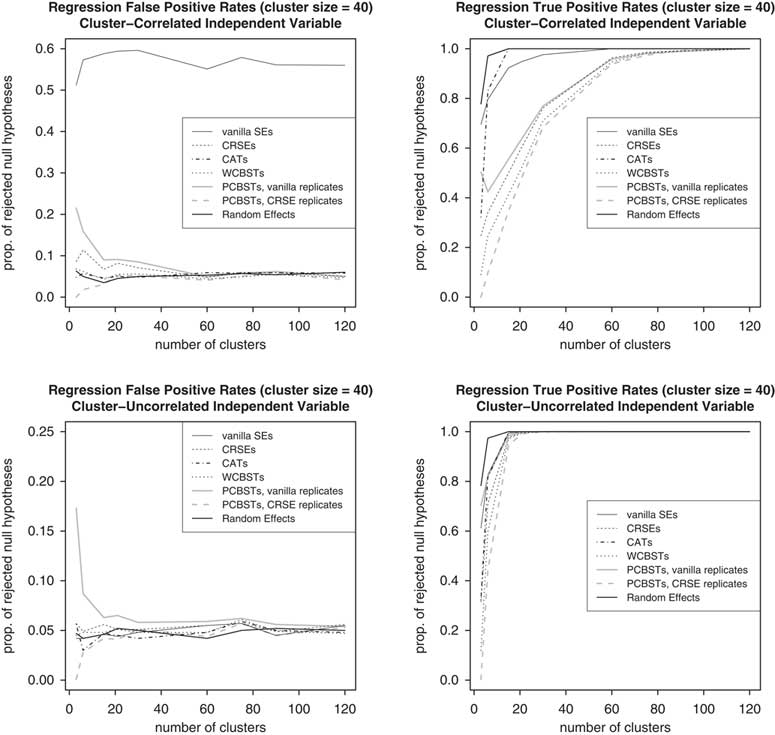
We begin with an assessment of size and power for a continuous dependent variable with no correlation between μ g and γ g ; these are shown in Figure 1. As the plots show, the ordinary SEs produced by glm (referred to as vanilla SEs in the figure) produce excess false positives for the cluster-correlated independent variable x when β x =0. On the other hand, the same SEs have a false positive rate for the cluster-uncorrelated variable z that is a good match for the α=0.05 value of the test. CRSEs produce excess false positives for G≤30 for both x and z but not for G≥60. These results are consistent with the prior findings of Angrist and Pischke (Reference Angrist and Pischke2009), Cameron, Gelbach and Miller (Reference Cameron, Gelbach and Miller2008), and Harden (Reference Harden2011).Footnote 16
Size and power assessment for linear dependent variables Note: The graphs on the left show the proportion of rejected null hypotheses (β=0) out of 1000 simulations for parameters whose true values are β x =β z =0 in the linear model y i =β x x i+ β z z i+ β w w i +γ g+ ε i with cluster dependency; this is a measure of the false positive rate. Each model (except random effects) is a correctly specified linear link generalized linear model (estimated using glm) with a different method of calculating statistical significance, as indicated in the legend; random effects models are correctly specified linear random effects models estimated using lme4. The hypothesis tests are conducted at α=0.05, so the false positive rate should ideally equal 0.05. The top graph shows the false positive rate for a variable (x) that is correlated with the cluster structure, while the bottom graph shows the false positive rate for a variable (z) that is uncorrelated with the cluster structure by design. The graphs on the right show the proportion of rejected null hypotheses out of 1000 simulations for parameters whose true values are β x =β z =0.25 in the same linear model; this is a measure of the true positive rate. One simulation is dropped for random effects models with 60 clusters due to estimation failure and the rejection rate is calculated out of 999 simulations for that case. For a method to have adequate power to conduct significance tests, the true positive rate should ideally equal 1. The top graph shows the true positive rate for a variable (x) that is correlated with the cluster structure, while the bottom graph shows the true positive rate for a variable (z) that is uncorrelated with the cluster structure by design. SEs=standard error; CRSE=cluster-robust standard error; CATs=cluster-adjusted t-statistics; WCBSTs=wild cluster bootstrapped t-statistics; PCBSTs=pairs cluster bootstrapped t-statistics.

PCBSTs offer better false positive performance than vanilla SEs or CRSEs for ≤21 clusters, but only when CRSE replicates are used. The proportion of rejected null hypotheses is close to the nominal 5 percent value of the test when using the CRSE replicates, except for very small numbers of clusters (where the rejection rate is lower than 5 percent). But this improvement in false positive performance is offset by worse performance in the detection of true positives, which is the worst for PCBSTs with CRSE replicates compared to any of the other options that we considered.
WCBSTs have false positive rates close to the target α=0.05 for even the smallest number of clusters. On the other hand, the true positive detection performance of WCBSTs is worse than all other techniques except PCBSTs with CRSE replicates. For the cluster-correlated independent variable, just over 70 percent of estimated
 $$\hat{\beta }_{x} $$
values are statistically significant when the true β
x
=0.25 when there are 30 clusters (for a total sample size of 1200 observations).
The CATs based on Ibragimov and Müller (Reference Ibragimov and Müller2010) have false positive rates that are close to the 5 percent α value of the test with appropriate size over the entire range of G. The CATs are also substantially better than all the other cluster-correction options we examine in terms of the power of hypothesis tests to detect true positives. While power is diminished for all the techniques for small numbers of clusters, the CATs achieve near-100 percent power rates more quickly than any of the clustering alternatives.
The best performance is achieved by RE models, which maintain a 5 percent false positive rate across the entire range of G and also achieve extremely high true positive detection rates at even the very smallest number of clusters. While there is little difference between CAT and RE true positive or false positive detection rates when the number of clusters is ≥15, for three or six clusters the RE model’s true positive performance is substantially better, ≈78 percent even with only three clusters.
Simulation Results for Linear Models With μ g /γ g Correlation and Serial Dependence
The performance of the RE estimator (shown in Figure 2) is substantially worsened when the data-generating process includes (a) correlation between the average value of x and the group effect γ g and (b) serial dependence in x and y. In this environment, the RE model produces a false positive for the cluster-correlated independent variable ≈70 percent of the time for all values of G, even worse than a fixed effects model with vanilla SEs in terms of excess false positive results. CRSEs, WCBSTs, and both forms of PCBSTs all perform better than these two options, but tend to over-reject the null hypothesis for G≤15. CATs have a false positive rate near 5 percent across all values of G.
Size and power assessment for linear dependent variables with fixed effects and serial dependence Note: The graph on the left shows the proportion of rejected null hypotheses (β=0) out of 1000 simulations for parameters whose true values is β x =0 in the linear model y i =β x x i +β z z i +β w w i +γ g +ε i with (a) correlation between the group-specific mean of x (=μ g ) and the group-level effect γ g and (b) within-group serial dependence in ε and x; this is a measure of the false positive rate. Each model (except random effects) is a correctly specified linear fixed effects model estimated using plm with a different method of calculating statistical significance, as indicated in the legend; random effects models are linear random effects models with correct variable specification (but no fixed effects) estimated using lme4. The hypothesis tests are conducted at α=0.05, so the false positive rate should ideally equal 0.05. The graph on the right shows the proportion of rejected null hypotheses out of 1000 simulations for parameters whose true values are β x =0.25 in the same linear model; this is a measure of the true positive rate. For a method to have adequate power to conduct significance tests, the true positive rate should ideally equal 1. See the Online Appendix for results for the cluster-uncorrelated independent variable (z). SEs=standard error; CRSE=cluster-robust standard error; CATs=cluster-adjusted t-statistics; WCBSTs=wild cluster bootstrapped t-statistics; PCBSTs=pairs cluster bootstrapped t-statistics.

The power characteristics of all models with appropriate size characteristics (particularly fixed effects models with CATs) are substantially reduced in this simulation for the serially dependent and cluster-correlated variable x. However, power characteristics improve substantially when the signal is made stronger (relative to noiseFootnote 17 ) so that β x =β z =0.5. In this alternative environment, CATs achieve 78 percent detection of true positives with 21 clusters.
Summary of Binary and Multinomial Simulation Results
The results of our simulations for binary and multinomial dependent variables are broadly comparable to those for linear models: CATs and PCBSTs with CRSE replicates have appropriate false positive rates, even for small numbers of clusters, while the other options have elevated false positive rates in data sets with ≤30 clusters. CATs have better power performance than PCBSTs with CRSE replicates. Details on these simulation results are provided in an Online Appendix.
There is one important caveat: CATs cannot be calculated whenever any cluster has no variation on the dependent variable, which can often occur with a categorical dependent variable. In addition, these models often produce a small number of outlying cluster coefficient estimates; this can happen, for example, when an independent variable perfectly predicts the dependent variable. We handle these problems by dropping clusters with missing and outlying estimates and calculating the CATs using the number of clusters that are not dropped. Theoretically, this corresponds to the idea that the dropped clusters contain no information and the remaining clusters still have the same distribution.Footnote 18 We provide an analytic argument in the Online Appendix that dropping these clusters will not distort inferences in many cases, particularly if the number of dropped clusters is relatively small. By dropping the clusters with missing and/or outlying estimates, we are able to estimate CATs on every data set with more than six clusters in our simulationFootnote 19 and our false positive rate remains very close to the nominal value of 5 percent with good power characteristics. We describe the practical consequences of dropping (and not dropping) clusters from the CAT procedure in greater detail in an Online Appendix.
APPLIED EXAMPLES
Our simulation results indicate that how we handle clustered data with a small number of clusters can greatly affect our inferences, and close examination of recently published examples of the analysis of clustered data underscores this finding. To this end, we re-analyzed the results of three recent publications that used CRSEs in data with few clusters: Grosser, Reuben and Tymula (Reference Grosser, Reuben and Tymula2013), Lacina (Reference Lacina2014), and Hainmueller, Hiscox and Sequeira (Reference Hainmueller, Hiscox and Sequeira2015). In each case, our reanalysis using alternative cluster corrections yields meaningfully different results. To save space, we describe the Grosser, Reuben and Tymula (Reference Grosser, Reuben and Tymula2013) replication in detail and only summarize the findings from Lacina (Reference Lacina2014) and Hainmueller, Hiscox and Sequeira (Reference Hainmueller, Hiscox and Sequeira2015); the details of these replications are present in an Online Appendix.
Political Quid Pro Quo Agreements (Grosser, Reuben and Tymula Reference Grosser, Reuben and Tymula2013)
In a recent AJPS article, Grosser, Reuben and Tymula (Reference Grosser, Reuben and Tymula2013) conduct a laboratory experiment designed to study the relationship between contributions to political candidates and the policies that are enacted by those candidates. In the experiment, a subject’s wealth endowment is randomly assigned by the experimenters; one “rich” voter is grouped with three “poor” voters, with the rich voter having 13 times more money than each of the poor voters; two non-voting “candidate” subjects are also assigned to the group. In the experimental condition that we study in this replication, groups are fixedFootnote
20
for the duration of the experiment; 17 such groups are present in the data set. The rich voter is allowed to give some of his or her own endowment to each of the two candidate subjects; we denote the rich voter’s monetary transfer to candidate i as m
i
. After receiving these transfers, each candidate i publicly proposes a redistributive tax rate τ
i
between 0 and 100 percent. The rich voter and the three poor voters then choose a candidate via majority vote; the selected candidate receives a fixed bonus payoff for winning. The winning candidate’s proposal (
 $$\tau ^{{\star}} $$
) is adopted: each voter pays
 $$\tau ^{{\star}} $$
percent of their income into a common fund, which is divided evenly among the voters. Thus, a voter with initial endowment e stands to lose
 $$\tau ^{{\star}} (e\,{\minus}\,\bar{e})$$
if rich, and gain
 $$\tau ^{{\star}} (\bar{e}\,{\minus}\,e)$$
if poor;
 $$\bar{e}$$
is the average endowment among all four voters in the group. This process is repeated in each of 15 periods. Explicit agreements can neither be made nor enforced in the experiment; for example, the rich voter cannot condition his or her donation on candidate behavior. Thus, any relationship between the transfers of the rich voter and the candidates’ tax proposals must be the result of a tacit agreement.
Grosser, Reuben and Tymula (Reference Grosser, Reuben and Tymula2013, figure 2) show a strong relationship between lower proposed tax rates and higher transfers to candidates from the rich voter despite electoral competition and the majority’s strong interest in complete redistribution. They are also interested in how these tacit agreements are formed, speculating that rich voters might first offer high transfers that are then reciprocated by lowered tax proposals. As they explain on page 591:
Are tacit agreements the result of mutual reciprocation between the rich voter and the two candidates? To answer this question, we use regression analysis to test whether changes in transfers can predict subsequent changes in tax policies and vice versa.
That is, they run a regression modeling the change in a candidate i’s proposed tax rate between period t and the previous period t−1, Δ
it
τ
=τ
it
−τ
i(t−1), that is associated with a change in the transfer received by that candidate from the rich voter between t and t−1, Δ
it
m
=m
it
−m
i(t−1). The authors also include a period counter t and interact Δ
it
m
with t in order to determine whether tacit agreements unravel over time. The difference between each candidate’s previous tax choice and the opponent’s choice, τ
i(t−1)−τ
j(t−1), is included as two variables, one for a positive difference
 $$\big(D_{{ij}}^{{\plus}} {\equals}\max \left( {\tau _{{i(t{\minus}1)}} \,{\minus}\,\tau _{{j(t{\minus}1)}} ,0} \right)\big)$$
and one for a negative difference
 $$\big (D_{{ij}}^{{\minus}} {\equals}\max \left( {\tau _{{j(t{\minus}1)}} {\minus}\tau _{{i(t{\minus}1)}} ,0} \right)\big )$$
; these variables are designed to study how candidates react to one another’s’ proposals.
The regression analysis of Grosser, Reuben and Tymula (Reference Grosser, Reuben and Tymula2013) uses CRSE calculated on the 17 groups of subjects; there are two candidate observations per group in each of 14 periods (excluding the first period, as changes are undefined for that period) for a total of 476 observations in the data set (28 total observations per group). The authors report strong evidence that “candidates do reciprocate the actions of the rich by decreasing (increasing) their tax policies in proportion to a previous increase (decrease) in received transfers (the coefficient of [Δ it m ] is always statistically significant)” (Grosser, Reuben, and Tymula, Reference Grosser, Reuben and Tymula2013; 592). However, the authors also report considerable group-to-group heterogeneity; tacit agreements between rich voters and candidates to exchange transfers for low tax rates evidently did not emerge in every experimental group (590–591).Footnote 21
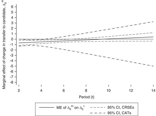
It is possible that uncertainty in the relationship between changes in transfers and changes in proposals might be understated by CRSE on data with only 17 groups. Therefore, we reproduce the regression analysis of Grosser, Reuben and Tymula (Reference Grosser, Reuben and Tymula2013) using their original CRSEs as well as PCBSTs and CATs. A marginal effect plot (see Brambor, Clark and Golder Reference Brambor, Clark and Golder2006) (Figure 3) for the marginal effect of changes in transfers on changes in tax policy in each period using these resultsFootnote 22 shows that the relationship is statistically significant in periods 2–6 using CRSEs, but only in periods 3 and 4 using CATs.
Marginal effects (ME) plot, effect of changed in received transfer (Δ it m ) on changes in proposed tax rate (Δ it τ ) by period Note: Dependent variable: change in candidate’s proposed tax rate (Δ it τ ). ME are calculated using the results in Online Appendix Table 2. CI=confidence interval; CRSE=cluster-robust standard error; CATs=cluster-adjusted t-statistics.

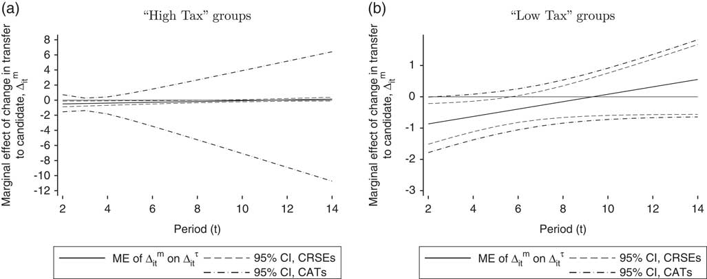
Grosser, Reuben and Tymula (Reference Grosser, Reuben and Tymula2013, 290) also separately examine the behavior of “high tax” groups, which have high winning tax policies (between 90 and 100 percent), and “low tax” groups, which have much lower winning tax policies (between 33.3 and 83.7 percent). We reproduce their analysis for high and low tax groups using CRSEs as well as PCBSTs and CATs; marginal effects plots for this analysis are shown in Figure 4.Footnote 23 For high tax groups, CRSEs indicate a statistically significant relationship between changes in transfers and changes in tax policy in periods 2–8. By comparison, CATs find no statistically significant relationship in any period.Footnote 24 For low tax groups, transfers are associated with lower tax proposals between periods 2 and 5 with CRSEs but are statistically indistinguishable from zero in every period except 2 with CATs.
Marginal effects (ME) plot, effect of changed in received transfer (Δ it m ) on changes in proposed tax rate (Δ it τ ) by period in high (a) and low tax groups (b) Note: Dependent variable: change in candidate’s proposed tax rate (Δ it τ ). ME are calculated using the results in Online Appendix Table 3 for panel 4 and Online Appendix Table 4 for panel 4. CI=confidence interval; CRSE=cluster-robust standard error; CATs=cluster-adjusted t-statistics.

In summary, although the evidence presented by Grosser, Reuben and Tymula (Reference Grosser, Reuben and Tymula2013) shows a possible link between Δ it m and Δ it τ , the statistical significance of this link is affected when we use CATs instead of CRSEs. The strong relationship the authors find between lower proposed tax rates and larger transfers from the rich voter might be explained by candidates reciprocating increased donations with decreased tax rates in low tax societies, but the experimental evidence for this explanation is more uncertain than CRSEs indicate.
Other Examples
Our replications of Lacina (Reference Lacina2014) and Hainmueller, Hiscox and Sequeira (Reference Hainmueller, Hiscox and Sequeira2015), described more fully in an Online Appendix, generally serve to reiterate the issues with using CRSEs with few clusters that are illustrated in the Grosser, Reuben and Tymula (Reference Grosser, Reuben and Tymula2013) replication. Lacina (Reference Lacina2014) uses a multinomial logit model and CRSEs to provide evidence for a link between political representation and civil unrest in India; specifically, she argues that linguistic groups that could have become Indian states were peacefully accommodated, ignored, or resorted to civil violence in relation to their representation in the Indian National Congress party. But the relationship between outcomes and representation that she describes is not robust to alternative methods of cluster adjustment for the SEs. More optimistically, we find that the substantive conclusion of Hainmueller, Hiscox and Sequeira (Reference Hainmueller, Hiscox and Sequeira2015) is robust to alternative clustering adjustments: based on their experiment, consumers are willing to pay more for products with a “fair trade” label. However, we also find that CRSEs understate the uncertainty of the substantive magnitude of this effect: estimated 95 percent confidence intervals are 20 percent wider when using PCBSTs and 46 percent wider when using CATs compared with the original results using CRSEs.
CONCLUSION
Political scientists often use CRSE to analyze clustered data where the structure of relationships inside of the cluster is uncertain or unknown. Unfortunately, past research indicates that CRSEs produce downward-biased SEs when the number of clusters is small; this can creates a hazard of excessive false positive results. Our research indicates that political scientists are still in the habit of using CRSEs in this scenario, possibly because alternatives are difficult to implement in common statistical packages.
Our findings and the prior literature suggest that substantive researchers should consider alternatives to the CRSE; we make it easy for them to do so with our clusterSEs package for R and the clustse and clusterbs ado files for Stata. Our simulation analysis finds that CATs (based on the work of Ibragimov and Müller Reference Ibragimov and Müller2010) are the best choice among the options we examine for correcting SEs for clustering in data sets with a small number of clusters. CATs require that a model must be separately estimable in every cluster, which is not always possible; however, dropping a small number of clusters where the model cannot be estimated and using the rest to estimate CATs can still produce valid inferences under many circumstances. If CATs cannot be estimated (e.g., because a key independent variable does not vary within clusters), PCBSTs with CRSE replicates and WCBST generally provide better performance than vanilla SEs or CRSEs. Finally, in our simulations an accurate RE model of intra-cluster heterogeneity provides better performance than any cluster adjustment technique, but the cluster adjustment techniques perform better in the event of misspecification.
Our final recommendation is that researchers think carefully about the amount of information contained in a data set with a small number of clusters, even if the number of observations in each cluster is large. If a researcher does not want to rely on assumptions about the structure of relationships inside of a cluster, then in some sense s/he is deciding to ignore the intra-cluster variation in the data set when estimating SEs. Political scientists would be wary of deriving strong conclusions from a data set with N=15 or 20 observations and five independent variables, even on the basis of a strongly statistically significant result. Based on our research and the findings of prior simulation studies, we believe that the same caution is warranted in the scenario with large N but only 15 or 20 clusters.