1 Introduction
The blood vessels of the microcirculation have diameters ranging between 5 and
 $20~\unicode[STIX]{x03BC}\text{m}$
, with a basal membrane (and, for arterioles a layer of smooth muscle), supporting endothelial cells (EC). These endothelial cells are coated with a layer of macromolecules referred to as the endothelial glycocalyx layer (EGL). This layer has an hydrated brush structure and is comprised of a large variety of membrane-bounded molecules including proteins, glycolipids (GL), glycoproteins (GP) and proteoglycans (PG) (Pries, Secomb & Gaehtgens Reference Pries, Secomb and Gaehtgens2000). It is believed that a principal function of the EGL is as a mechanotransducer of mechanical stresses to the underlying endothelial cells (Tarbell & Pahakis Reference Tarbell and Pahakis2006). However, due to the small scale of the EGL (about
 $1~\unicode[STIX]{x03BC}\text{m}$
) and its delicate nature, experimental investigation of the EGL in vivo is extremely challenging. Some sophisticated experimental techniques have been developed to investigate flow properties near the vessel wall (Pries et al.
Reference Pries, Secomb and Gaehtgens2000; Weinbaum, Tarbell & Damiano Reference Weinbaum, Tarbell and Damiano2007), however, mathematical and computational modelling remain a powerful tool to elucidate the EGL’s role and function.
There have been numerous theoretical and computational studies of the EGL. Some models have treated the EGL as rigid (Hariprasad & Secomb Reference Hariprasad and Secomb2012), others as deformable. In the latter case, biphasic mixture theory (BMT) has commonly been used to describe the poro-elastohydrodynamics of the EGL (Damiano et al. Reference Damiano, Duling, Ley and Skalak1996; Wei et al. Reference Wei, Waters, Liu and Grotberg2003; Damiano & Stace Reference Damiano and Stace2005; Sumets et al. Reference Sumets, Cater, Long and Clarke2015; Lee, Long & Clarke Reference Lee, Long and Clarke2016). In BMT, the EGL is modelled as an hydrated porous material that can be described at the macroscopic level by two spatially coincidental phases: a linearly elastic solid phase and a fluid phase. These earlier studies suggested the importance of the EGL in protecting the endothelial surface from excessive fluid shear stresses, by transmitting much of the applied mechanical load through the EGL’s solid matrix, rather than through the fluid phase. The effect of redistribution of the EGL to cell–cell junctions was also investigated by Lee et al. (Reference Lee, Long and Clarke2016), who found that it can have a noticeable influence upon the magnitude of the transmitted mechanical stresses.
It is worth noting that in these studies the EGL was considered to be electrically neutral, and any charged species within the fluid phase were ignored. However, the PG are naturally charged macromolecules and lead to an EGL that is negatively charged. Furthermore, blood plasma is a solution containing water as well as
 $\text{Na}^{+}$
and
 $\text{Cl}^{-}$
ions, which can electrically interact with the negatively charged EGL. Theoretical estimates show that under normal conditions the fixed charge concentration of the EGL is of the same order of magnitude as the physiological neutral salt concentration in blood plasma (
 ${\approx}0.1~\text{M}$
) (Silberberg Reference Silberberg1991). Hence, it is reasonable to expect that electrochemical interactions between the EGL and blood plasma could be important.
There has been some previous work investigating the effects of a charged EGL, with several different approaches adopted. Specifically, a charged surface model (Liu & Yang Reference Liu and Yang2009), a volume charge model (Stace & Damiano Reference Stace and Damiano2001; Damiano & Stace Reference Damiano and Stace2002) and a charged rod model (Buschmann & Grodzinsky Reference Buschmann and Grodzinsky1995; Mokady, Mestel & Winlove Reference Mokady, Mestel and Winlove1999). The charged surface model assumes that the EGL has zero thickness and the vessel wall carries the charge distribution. This approach does not consider the EGL structure and does not allow for consideration of EGL mechanics.
The charged rod model takes into account the particular spatially distributed electrical properties of the layer. On the molecular level the PG can be considered as a polyelectrolyte brush and the EGL is modelled as a doubly periodic array of parallel rigid charged cylinders surrounded by a Newtonian ionic fluid. Electrostatic forces arising in this model without background flow were investigated by Dean et al. (Reference Dean, Seog, Ortiz and Grodzinsky2003). It was found that molecular-level changes in the charge distribution inside polyelectrolyte brush layers can significantly change the magnitude and the shape of the resulting electrostatic force profile. The electrical effects of the EGL on the flow, streaming potential and electrophoretic mobility of red blood cells were considered by Mokady et al. (Reference Mokady, Mestel and Winlove1999) using the charged rod model. An important conclusion from this study is that streaming currents in the lumen are determined by the structure and behaviour of only the outermost portion of the glycocalyx. This model predicts that close to the surface of an EC (at the base of the EGL), the ion concentrations will be unaffected.
In a volume charge model (an averaged macro-level representation), the EGL is assumed to have an homogeneous solid matrix with a volume charge distribution. In this case triphasic mixture theory (TMT) can be used to mathematically describe the mechano-electrochemical EGL behaviour. It combines the physico-chemical theory for ionic and polyionic (proteoglycan) mixture with biphasic mixture theory for porous media. The result is an extended biphasic mixture theory formulation consisting of a fully saturated solid skeleton carrying fixed negative charges and an incompressible pore fluid containing mobile ions. Under TMT, fluid and solid phases are described by the Brinkman and Navier equations, respectively, subject to electric body forces. First principal derivations of such a multiphase model can be obtained from a micromechanical description, and can be found in the existing literature (e.g. Ehlers & Bluhm Reference Ehlers and Bluhm2002; Kolev Reference Kolev2002; Holzapfel & Ogden Reference Holzapfel and Ogden2006). TMT has been used in a number of different applications, that include (but not limited to) swelling of intervertebral disk (Ehlers, Karajan & Markert Reference Ehlers, Karajan and Markert2009), soil mechanics (Ehlers & Blome Reference Ehlers and Blome2003) and articular cartilage (Lai, Hou & Mow Reference Lai, Hou and Mow1991). These have also been a number of studies which have shown the predictions of TMT to be in good agreement with experimental data, including the deformation response of a hydrogel strip under an external electric field (Zhou et al. Reference Zhou, Hon, Sun and Mak2002), as well as the swelling of synthetic (Oomens et al. Reference Oomens, De Heus, Huyghe, Nelissen and Janssen1995) and real (Frijns, Huyghe & Janssen Reference Frijns, Huyghe and Janssen1997) intervertebral tissue under mechanical loading and different salinity conditions.
In the context of EGL modelling, a pseudo-equilibrium approximation of the TMT was used by Damiano & Stace (Reference Damiano and Stace2002) to predict the recovery time of the glycocalyx after the passing of a stiff leukocyte. It was shown that a fixed charge density would result in a voltage differential between the undeformed glycocalyx and the capillary lumen of 0.1 mV. Under compression of the EGL a repulsive electrostatic force restores the EGL to its undeformed thickness. The analysis reveals that the magnitude of the glycocalyx restoring force can be attenuated by increasing (or amplified by decreasing) the concentration of mobile cations in the plasma. However, this study did not analyse the influence of the flow through the vessel upon the dynamics, which can introduce a streaming potential in the vessel. The streaming potential and hydrodynamics of surfaces covered with charged layers were studied by Donath & Voigt (Reference Donath and Voigt1986) (in a non-EGL context) using the nonlinear Poisson–Boltzmann equation for the electric potential, which assumes an electroneutral balance between the charged EGL and the ions. Under this assumption, it was demonstrated that surfaces with charged layers can have extraordinarily high surface conductivities when this layer becomes thicker.
TMT has been successfully employed to describe the influence and behaviour of a charged EGL in a limited number of situations, predominantly under the assumption of electroneutrality. However, the electroneutrality condition, which predicts a Boltzmann distribution for ion concentrations, is not necessarily valid in the presence of a background pressure-driven flow that can transport the ions (as would be the case in a microvessel). A study of the full problem incorporating the interplay between charged ions, a deformable charged EGL and a background viscous flow has not been yet undertaken. Therefore, in what follows we consider pressure-driven flow of an ionised fluid through a charged and deformable EGL which coats the internal surface of vessel with slowly changing geometry. This extends the earlier work of Damiano & Stace (Reference Damiano and Stace2002) where the background fluid flow is neglected and a pseudo-equilibrium approximation along with an electroneutrality condition is invoked, and enables us to investigate the combined effects of geometry and charge upon the hemodynamics.
In § 2 we introduce the modelling assumptions and governing equations, along with the necessary boundary conditions. Scalings within the non-dimensionalised equations suggest the presence of a thin transitional layer (Debye layer) for ion concentrations and electrical potentials, which we treat asymptotically in § 3. This analysis provides jump conditions for the dynamics in the bulk EGL/lumen, which we solve using a hybrid boundary–finite element method scheme described § 4. This allows us to solve the dynamics numerically within arbitrarily shaped geometries for physiologically realistic parameter values. In § 5 we present predictions for the influence of charge effects upon flow profiles and endothelial shear stresses, which are further discussed in § 6.
2 Formulation
We treat the EGL as a charged poroelastic layer which allows us to account for the fact that the proteoglycan chains have a net negative electrical charge. Blood plasma is a solution of many different mobile charged ions, of which sodium (
 $\text{Na}^{+}$
) and chloride (
 $\text{Cl}^{-}$
) are by far the most abundant, and hence the ones that we restrict attention to here. These are transported by a pressure-driven flow through the microvessel, which results in electrical fields being generated within the microvessel.
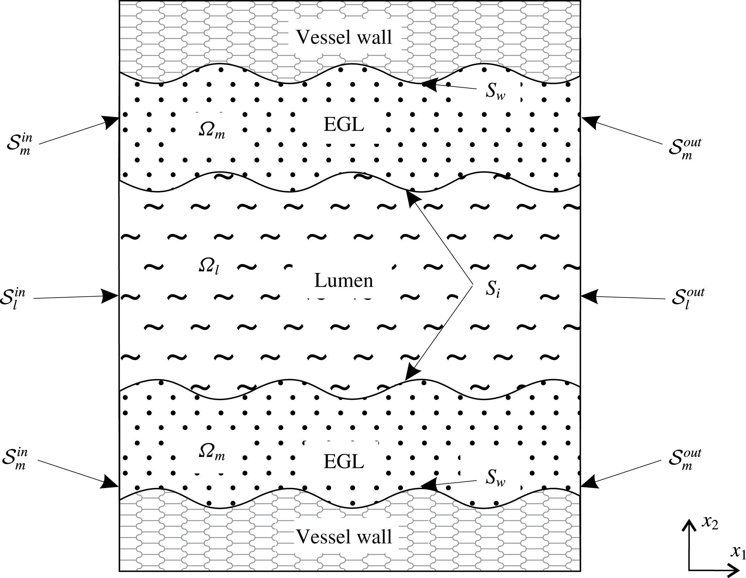
Figure 1 shows an annotated sketch of the vessel geometry and the electro-poroelasticity that is modelled using triphasic mixture theory (TMT). We use coordinates
 $x_{1}$
and
 $x_{2}$
to indicate streamwise and cross-stream positions, respectively. Our findings focus on the shear stresses exerted on the vessel wall due to the solid and fluid phases, and the implications for the mechanotransduction role of the EGL. It is also of interest to compare the predictions made by TMT against those made by BMT as a means of gauging the impact of charge effects upon microvessel mechanics.
A sketch of two-dimensional wavy wall channel lined with a charged poroelastic EGL. This is annotated with the definitions for the various surfaces and volumes, e.g.
 ${\mathcal{S}}_{l}^{in}$
and
 $\unicode[STIX]{x1D6FA}_{l}$
for luminal inlet and interior, respectively.
2.1 Model assumptions
Using TMT, the EGL region is modelled as a multicomponent material consisting of water, the electrostatically charged elastic solid matrix and mobile ions (
 $\text{Na}^{+}$
and
 $\text{Cl}^{-}$
). Water and ions combined together form a fluid phase (blood plasma). As a result, there are four volume fractions associated with each phase, namely, the solid fraction
 $\unicode[STIX]{x1D719}_{s}$
, water fraction
 $\unicode[STIX]{x1D719}_{w}$
as well as cation and anion fractions (
 $\unicode[STIX]{x1D719}_{+}$
and
 $\unicode[STIX]{x1D719}_{-}$
, respectively). The fluid phase is therefore comprised of three constituents
 $\unicode[STIX]{x1D719}_{f}=\unicode[STIX]{x1D719}_{w}+\unicode[STIX]{x1D719}_{+}+\unicode[STIX]{x1D719}_{-}$
. Mass conservation dictates that
 $\unicode[STIX]{x1D719}_{s}+\unicode[STIX]{x1D719}_{f}=1$
.
The model is based on the following assumptions.
-
(i) We assume that
 $\unicode[STIX]{x1D719}_{w}\approx \unicode[STIX]{x1D719}_{f}$
. This assumption is valid for dilute solutions (Damiano & Stace Reference Damiano and Stace2002; Masliyah & Bhattacharjee Reference Masliyah and Bhattacharjee2006). Indeed, the physiological value of salt concentration in blood plasma under normal conditions is
$0.15~\text{mol}~\text{l}^{-1}$
. In this case
$\unicode[STIX]{x1D719}_{\pm }\ll \unicode[STIX]{x1D719}_{w}$
and the ions in solution can be treated as point charges. This dilute assumption has been shown to be valid provided that the ion concentrations do not approach the ion packing fraction, i.e.
$c^{\ast }\sim 1/a^{\ast 3}$
, where
$a^{\ast }=O(10^{-10}~\text{m})$
is the ionic radius (Kilic & Bazant Reference Kilic and Bazant2007).
-
(ii) The flow is pressure driven and there are no externally applied electric fields or ion concentration gradients. Due to the small scale nature of the flow in microvessels, we make the usual assumptions that the flow is steady state and gravitational and inertia forces are negligible (Wei et al. Reference Wei, Waters, Liu and Grotberg2003; Sumets et al. Reference Sumets, Cater, Long and Clarke2015; Lee et al. Reference Lee, Long and Clarke2016). For example, in our particular case, the characteristic velocity
$V^{\ast }$
is of order
$10^{-3}~\text{m}~\text{s}^{-1}$
, microvessel radius is
$H^{\ast }=5\times 10^{-6}~\text{m}$
and fluid density
$\unicode[STIX]{x1D70C}^{\ast }$
and viscosity
$\unicode[STIX]{x1D707}_{f}^{\ast }$
take values similar to that of water, which gives a Reynolds number of
$Re=O(10^{-3})$
. -
(iii) The electric field arising from the presence of charged components relates to the bulk mixture which is the volume average over the fluid, solid and ion phases (Damiano & Stace Reference Damiano and Stace2002). Strictly speaking, each charged constituent (ions and solid matrix) of the EGL generates its own electric field contributing to the total electrostatic effect. We consider the total electric field. This means that the term electroneutrality denotes zero net charge in the bulk mixture (fluid and solid phases together).
-
(iv) The electrostatic effect of the solid matrix arising from the presence of charged PG chains in the EGL is characterised by the concentration of charged molecules
$c_{s}^{\ast }$
fixed in the solid phase. Following Damiano & Stace (Reference Damiano and Stace2002), we employ a volume charge model and assume that the solid phase is charged volumetrically with
$c_{s}^{\ast }$
constant. This assumption implies that there is no surface charge concentration on the interface between the lumen and EGL. -
(v) Deformations of the EGL are induced by the background flow and electrostatic fields. Small strain theory is used for the elastic deformation and we do not consider any large strain deformations of the EGL which might be caused by, for example, crushing of the layer by large white blood cells. Therefore, any changes in the electric field resulting from changes in the solid volume fraction are neglected. The EGL is attached to an immovable rigid wall and, therefore, the velocity of the solid phase is equal to zero,
$\boldsymbol{v}_{s}^{\ast }=0$
. -
(vi) We assume that the vessel walls are impermeable, so that there is no transmural flux of plasma or ions capable of generating a net current in the vessel.
-
(vii) We consider vessels which are comparable in diameter to transiting cells. In this case, if included, cells must be modelled explicitly, rather than via a non-Newtonian flow or two-layer viscosity model (Sharan & Popel Reference Sharan and Popel2001; Lee et al. Reference Lee, Long and Clarke2016) (although we do not do so here). The remaining plasma is over
$92\,\%$
water, which we consequently model as a Newtonian fluid. -
(viii) Dielectric permittivity is the same everywhere as that of the bulk solution and is independent of the electric field (Damiano & Stace Reference Damiano and Stace2002).








2.2 Dynamics in the lumen (triphasic)
Following the theory of mixtures (Ehlers & Bluhm Reference Ehlers and Bluhm2002) we model the blood plasma in the lumen as an isotropic fluid of three components – water (
 $w$
), anions (
 $-$
) and cations (
 $+$
), with volume fractions
 $\unicode[STIX]{x1D719}_{\unicode[STIX]{x1D6FC}}$
,
 $\unicode[STIX]{x1D6FC}=\{w,-,+\}$
, so that
 $\unicode[STIX]{x1D719}_{w}+\unicode[STIX]{x1D719}_{+}+\unicode[STIX]{x1D719}_{-}=1$
. Densities
 $\unicode[STIX]{x1D70C}_{w}^{\ast }=\unicode[STIX]{x1D719}_{w}{\unicode[STIX]{x1D70C}^{\ast }}_{w}^{T}$
,
 $\unicode[STIX]{x1D70C}_{\pm }^{\ast }=\unicode[STIX]{x1D719}_{\pm }{\unicode[STIX]{x1D70C}^{\ast }}_{\pm }^{T}=M_{\pm }^{\ast }c_{l\pm }^{\ast }$
where
 ${\unicode[STIX]{x1D70C}^{\ast }}_{\unicode[STIX]{x1D6FC}}^{T}$
is the true (intrinsic) density,
 $M_{\pm }^{\ast }$
is a molecular weight and
 $c_{l\pm }^{\ast }=c_{l\pm }^{\ast }(\boldsymbol{x})$
is an ionic concentration in the lumen. The velocity of the mixture in lumen
 $\boldsymbol{v}_{l}^{\ast }$
can be written in terms of the velocities of the components as
 $$\begin{eqnarray}\boldsymbol{v}_{l}^{\ast }=\unicode[STIX]{x1D719}_{w}\boldsymbol{v}_{lw}^{\ast }+\unicode[STIX]{x1D719}_{+}\boldsymbol{v}_{l+}^{\ast }+\unicode[STIX]{x1D719}_{-}\boldsymbol{v}_{l-}^{\ast }.\end{eqnarray}$$
For dilute systems
 $\unicode[STIX]{x1D719}_{\pm }\ll 1$
, consequently
 $\boldsymbol{v}_{l}^{\ast }\approx \boldsymbol{v}_{lw}^{\ast }$
and
 $\unicode[STIX]{x1D719}_{w}\approx 1$
, so the fluid velocity is approximately equal to the velocity of the water component.
The charge density in the lumen
 $q_{l}^{\ast }$
is defined as
 $$\begin{eqnarray}q_{l}^{\ast }=e^{\ast }z_{+}c_{l+}^{\ast }+e^{\ast }z_{-}c_{l-}^{\ast },\end{eqnarray}$$
where
 $z_{\pm }=\pm 1$
are ion valences and
 $e^{\ast }$
is the elementary charge.
Mass conservation
Conservation of mass (assuming no chemical reactions) for each component requires
 $$\begin{eqnarray}\unicode[STIX]{x1D735}^{\ast }\boldsymbol{\cdot }\boldsymbol{v}_{l}^{\ast }=0,\quad \unicode[STIX]{x1D735}^{\ast }\boldsymbol{\cdot }(c_{l\pm }^{\ast }\boldsymbol{v}_{l\pm }^{\ast })=0.\end{eqnarray}$$
From (2.3) we immediately obtain conservation of charge. Indeed, the individual fluxes of both ionic species result in a net current,
 $\boldsymbol{i}_{l}^{\ast }$
 $$\begin{eqnarray}\boldsymbol{i}_{l}^{\ast }=e^{\ast }c_{l+}^{\ast }\boldsymbol{v}_{l+}^{\ast }-e^{\ast }c_{l-}^{\ast }\boldsymbol{v}_{l-}^{\ast }.\end{eqnarray}$$
Expressions (2.3) and (2.4) yield
 $\unicode[STIX]{x1D735}^{\ast }\boldsymbol{\cdot }\boldsymbol{i}_{l}^{\ast }=0$
.
Momentum conservation
Considering the fluid as a dielectric containing mobile ions, the flow momentum equation for Newtonian fluid without inertia is given by
 $$\begin{eqnarray}\unicode[STIX]{x1D735}^{\ast }\boldsymbol{\cdot }\unicode[STIX]{x1D748}_{l}^{\ast }+\boldsymbol{F}_{l}^{\ast }=0,\end{eqnarray}$$
where
 $\unicode[STIX]{x1D748}_{l}^{\ast }=-p_{l}^{\ast }\unicode[STIX]{x1D644}+\unicode[STIX]{x1D707}_{f}^{\ast }(\unicode[STIX]{x1D735}^{\ast }\boldsymbol{v}_{l}^{\ast }+(\unicode[STIX]{x1D735}^{\ast }\boldsymbol{v}_{l}^{\ast })^{\text{T}})$
is a Newtonian stress tensor,
 $p_{l}^{\ast }$
is the hydrodynamic pressure in the lumen, and
 $\boldsymbol{F}_{l}^{\ast }$
is a body force. This force includes an electric force
 $\boldsymbol{Q}_{l}^{\ast }$
due to the electric field
 $\boldsymbol{E}_{l}^{\ast }$
and an osmotic pressure due to free ions
 ${\mathcal{P}}_{l}^{\ast }$
, so that
 $\boldsymbol{F}_{l}^{\ast }=\unicode[STIX]{x1D735}^{\ast }{\mathcal{P}}_{l}^{\ast }+\boldsymbol{Q}_{l}^{\ast }$
. We assume that the ions behave like an ideal gas (Damiano & Stace Reference Damiano and Stace2002) and the osmotic pressure is analogous to the ideal gas law
 ${\mathcal{P}}_{l}^{\ast }=-(c_{l+}^{\ast }+c_{l-}^{\ast })k^{\ast }T^{\ast }$
, where
 $k^{\ast }$
is Boltzmann’s constant and
 $T^{\ast }$
is the absolute temperature. The electric body force per unit volume in the dielectric medium is given by (Landau & Lifshitz Reference Landau and Lifshitz1960)
 $$\begin{eqnarray}\boldsymbol{Q}_{l}^{\ast }=-e^{\ast }(c_{l+}^{\ast }-c_{l-}^{\ast })\unicode[STIX]{x1D735}^{\ast }\unicode[STIX]{x1D711}_{l}^{\ast },\end{eqnarray}$$
where
 $\unicode[STIX]{x1D711}_{l}^{\ast }$
is the electric potential. As a result, (2.5) takes the form
 $$\begin{eqnarray}\unicode[STIX]{x1D707}_{f}^{\ast }{\unicode[STIX]{x1D6FB}^{\ast }}^{2}\boldsymbol{v}_{l}^{\ast }=\unicode[STIX]{x1D735}^{\ast }p_{l}^{\ast }+\unicode[STIX]{x1D735}^{\ast }(c_{l+}^{\ast }+c_{l-}^{\ast })k^{\ast }T^{\ast }+e^{\ast }(c_{l+}^{\ast }-c_{l-}^{\ast })\unicode[STIX]{x1D735}^{\ast }\unicode[STIX]{x1D711}_{l}^{\ast }.\end{eqnarray}$$
Combining the osmotic pressure term
 $(c_{l+}^{\ast }+c_{l-}^{\ast })k^{\ast }T^{\ast }$
with the hydrodynamic pressure
 $p_{l}^{\ast }$
yields the total pressure, but we consider them separately to highlight the difference in the nature of these pressures.
Gauss’s law
Under the constant permittivity assumption, the electric field can be related to the total volume space charge density using Gauss’s law (Landau & Lifshitz Reference Landau and Lifshitz1960)
 $$\begin{eqnarray}-\unicode[STIX]{x1D716}^{\ast }{\unicode[STIX]{x1D6FB}^{\ast }}^{2}\unicode[STIX]{x1D711}_{l}^{\ast }=e^{\ast }(c_{l+}^{\ast }-c_{l-}^{\ast }),\end{eqnarray}$$
with
 $\unicode[STIX]{x1D716}^{\ast }$
being a dielectric permittivity.
Ion transport
Ion transport is described by the Nernst–Planck equation for dilute ionic solutions (Masliyah & Bhattacharjee Reference Masliyah and Bhattacharjee2006)
 $$\begin{eqnarray}c_{l\pm }^{\ast }\boldsymbol{v}_{l\pm }^{\ast }=\boldsymbol{v}_{l}^{\ast }c_{l\pm }^{\ast }-D_{\pm }^{\ast }\unicode[STIX]{x1D735}^{\ast }c_{l\pm }^{\ast }\mp \frac{e^{\ast }\unicode[STIX]{x1D735}^{\ast }\unicode[STIX]{x1D711}_{l}^{\ast }}{k^{\ast }T^{\ast }}D_{\pm }^{\ast }c_{l\pm }^{\ast },\end{eqnarray}$$
where
 $D_{\pm }^{\ast }$
are the diffusivities of the positive and negative ions (cations and anions), respectively. Expression (2.9) shows that the mass flux of a solute species is a combination of the flux due to a background flow, the flux due to the concentration gradient (i.e. diffusional process), and the flux due to bulk convection. The Nernst–Planck equation can lead to predictions of local concentrations that are sufficiently high so as to invalidate the neglect of steric interactions in the model (Kilic & Bazant Reference Kilic and Bazant2007). In such situations a modified Nernst–Planck model can be adopted, however, we shall see in § 5 that we do not approach that regime at any point.
Overall, we obtain seven equations (2.3), (2.7), (2.8), (2.9) for the seven unknowns
 $\boldsymbol{v}_{l}^{\ast }$
,
 $p_{l}^{\ast }$
,
 $\unicode[STIX]{x1D711}_{l}^{\ast }$
,
 $c_{l+}^{\ast }$
,
 $c_{l-}^{\ast }$
,
 $\boldsymbol{v}_{l+}^{\ast }$
,
 $\boldsymbol{v}_{l-}^{\ast }$
. Substitution of (2.9) into (2.3) enables us to eliminate
 $\boldsymbol{v}_{l+}^{\ast }$
and
 $\boldsymbol{v}_{l-}^{\ast }$
from the system. We arrive at the equations
 $$\begin{eqnarray}\displaystyle & \displaystyle \unicode[STIX]{x1D707}_{f}^{\ast }{\unicode[STIX]{x1D6FB}^{\ast }}^{2}\boldsymbol{v}_{l}^{\ast }=\unicode[STIX]{x1D735}^{\ast }p_{l}^{\ast }+\unicode[STIX]{x1D735}^{\ast }(c_{l+}^{\ast }+c_{l-}^{\ast })k^{\ast }T^{\ast }+e^{\ast }(c_{l+}^{\ast }-c_{l-}^{\ast })\unicode[STIX]{x1D735}^{\ast }\unicode[STIX]{x1D711}_{l}^{\ast }, & \displaystyle\end{eqnarray}$$
 $$\begin{eqnarray}\displaystyle & \displaystyle \unicode[STIX]{x1D735}^{\ast }\boldsymbol{\cdot }\boldsymbol{v}_{l}^{\ast }=0, & \displaystyle\end{eqnarray}$$
 $$\begin{eqnarray}\displaystyle & \displaystyle \boldsymbol{v}_{l}^{\ast }\boldsymbol{\cdot }\unicode[STIX]{x1D735}^{\ast }c_{l\pm }^{\ast }-D_{\pm }^{\ast }{\unicode[STIX]{x1D6FB}^{\ast }}^{2}c_{l\pm }^{\ast }\mp \frac{e^{\ast }D_{\pm }^{\ast }}{k^{\ast }T^{\ast }}\unicode[STIX]{x1D735}^{\ast }\boldsymbol{\cdot }(c_{l\pm }^{\ast }\unicode[STIX]{x1D735}^{\ast }\unicode[STIX]{x1D711}_{l}^{\ast })=0, & \displaystyle\end{eqnarray}$$
 $$\begin{eqnarray}\displaystyle & \displaystyle -\unicode[STIX]{x1D716}^{\ast }{\unicode[STIX]{x1D6FB}^{\ast }}^{2}\unicode[STIX]{x1D711}_{l}^{\ast }=e^{\ast }(c_{l+}^{\ast }-c_{l-}^{\ast }), & \displaystyle\end{eqnarray}$$
which model the dynamics in the lumen.
2.3 Dynamics in the EGL (triphasic)
In the EGL itself there is an additional solid phase with volume fraction
 $\unicode[STIX]{x1D719}_{s}$
so that
 $\unicode[STIX]{x1D719}_{f}+\unicode[STIX]{x1D719}_{s}=1$
, and
 $\unicode[STIX]{x1D719}_{f}\approx \unicode[STIX]{x1D719}_{w}$
is the fluid fraction. We consider small strains, which means that while the solid matrix can deform, there are no appreciable volumetric changes. Since mixture theory assumes an homogeneous, isotropic material structure, this implies that
 $\unicode[STIX]{x1D719}_{s}$
can be assumed to be constant (both in time, and spatially).
Assuming steady flow and zero solid phase velocity we have mass conservation for the mixture
 $$\begin{eqnarray}\unicode[STIX]{x1D735}^{\ast }\boldsymbol{\cdot }\boldsymbol{v}_{f}^{\ast }=0,\quad \unicode[STIX]{x1D735}^{\ast }\boldsymbol{\cdot }(c_{f\pm }^{\ast }\boldsymbol{v}_{f\pm }^{\ast })=0,\end{eqnarray}$$
where
 $\boldsymbol{v}_{f\pm }^{\ast }$
are the velocities of ions in the fluid phase of the EGL,
 $c_{f\pm }^{\ast }$
are the ion concentrations in the EGL. As in the lumen, the latter implies conservation of current in the EGL
 $$\begin{eqnarray}\boldsymbol{i}_{f}^{\ast }=e^{\ast }c_{f+}^{\ast }\boldsymbol{v}_{f+}^{\ast }-e^{\ast }c_{f-}^{\ast }\boldsymbol{v}_{f-}^{\ast },\end{eqnarray}$$
i.e.
 $\unicode[STIX]{x1D735}^{\ast }\boldsymbol{\cdot }\boldsymbol{i}_{f}^{\ast }=0$
.
Modelling the poroelastohydrodynamics using biphasic mixture theory, the momentum equations for the fluid and solid components containing body forces are given by
 $$\begin{eqnarray}\displaystyle & \displaystyle \unicode[STIX]{x1D719}_{f}\unicode[STIX]{x1D735}^{\ast }\boldsymbol{\cdot }\unicode[STIX]{x1D748}_{f}^{\ast }+\unicode[STIX]{x1D719}_{f}\unicode[STIX]{x1D735}^{\ast }{\mathcal{P}}^{\ast }+\unicode[STIX]{x1D719}_{f}\boldsymbol{Q}_{f}^{\ast }=\unicode[STIX]{x1D745}^{\ast }, & \displaystyle\end{eqnarray}$$
 $$\begin{eqnarray}\displaystyle & \displaystyle \unicode[STIX]{x1D719}_{s}\unicode[STIX]{x1D735}^{\ast }\boldsymbol{\cdot }\unicode[STIX]{x1D748}_{s}^{\ast }+\unicode[STIX]{x1D719}_{s}\unicode[STIX]{x1D735}^{\ast }{\mathcal{P}}^{\ast }+\unicode[STIX]{x1D719}_{s}\boldsymbol{Q}_{s}^{\ast }=-\unicode[STIX]{x1D745}^{\ast }, & \displaystyle\end{eqnarray}$$
where
 $\unicode[STIX]{x1D748}_{f}^{\ast }=-p_{f}^{\ast }\unicode[STIX]{x1D644}+\unicode[STIX]{x1D707}_{f}^{\ast }(\unicode[STIX]{x1D735}^{\ast }\boldsymbol{v}_{f}^{\ast }+(\unicode[STIX]{x1D735}^{\ast }\boldsymbol{v}_{f}^{\ast })^{\text{T}})$
and
 $\unicode[STIX]{x1D748}_{s}^{\ast }=-p_{f}^{\ast }\unicode[STIX]{x1D644}+\unicode[STIX]{x1D707}_{s}^{\ast }(\unicode[STIX]{x1D735}^{\ast }\boldsymbol{u}^{\ast }+(\unicode[STIX]{x1D735}^{\ast }\boldsymbol{u}^{\ast })^{\text{T}})+\unicode[STIX]{x1D706}_{s}^{\ast }(\unicode[STIX]{x1D735}^{\ast }\boldsymbol{\cdot }\boldsymbol{u}^{\ast })\unicode[STIX]{x1D644}$
are the stress tensors for the fluid and solid phases respectively where
 $\boldsymbol{u}^{\ast }$
is the elastic displacement,
 $\boldsymbol{Q}_{f}^{\ast }=e^{\ast }(c_{f+}^{\ast }-c_{f-}^{\ast })\unicode[STIX]{x1D735}^{\ast }\unicode[STIX]{x1D711}_{f}^{\ast }$
and
 $\boldsymbol{Q}_{s}^{\ast }=e^{\ast }z_{s}c_{s}^{\ast }\unicode[STIX]{x1D735}^{\ast }\unicode[STIX]{x1D711}_{f}^{\ast }$
are the electric body forces,
 $\unicode[STIX]{x1D745}^{\ast }=K^{\ast }\boldsymbol{v}_{f}^{\ast }$
is the momentum transfer with
 $K^{\ast }$
being the hydraulic resistivity,
 $\unicode[STIX]{x1D711}_{f}^{\ast }$
is the electric potential in the EGL and
 $z_{s}$
is the valence of the PG molecules. Following Damiano & Stace (Reference Damiano and Stace2002) we associate the body force due to an electric field acting on the fluid fraction with mobile ion charges and the force acting on the solid phase with fixed charge concentration. The osmotic pressure
 ${\mathcal{P}}^{\ast }=-(c_{f+}^{\ast }+c_{f-}^{\ast })k^{\ast }T^{\ast }$
is split proportionally between phases, in a similar manner as for the hydrodynamic pressure
 $p^{\ast }$
.
The total charge in the EGL region is
 $q_{f}^{\ast }=\unicode[STIX]{x1D719}_{f}e^{\ast }(c_{f+}^{\ast }-c_{f-}^{\ast })+\unicode[STIX]{x1D719}_{s}z_{s}e^{\ast }c_{s}^{\ast }$
and Gauss’s law takes the form
 $$\begin{eqnarray}\displaystyle -\unicode[STIX]{x1D716}^{\ast }{\unicode[STIX]{x1D6FB}^{\ast }}^{2}\unicode[STIX]{x1D711}_{f}^{\ast }=e^{\ast }(\unicode[STIX]{x1D719}_{f}(c_{f+}^{\ast }-c_{f-}^{\ast })+\unicode[STIX]{x1D719}_{s}z_{s}c_{s}^{\ast }). & & \displaystyle\end{eqnarray}$$
As in the lumen, the Nernst–Planck equation is used to describe ion transport in the fluid phase of the EGL
 $$\begin{eqnarray}c_{f\pm }^{\ast }\boldsymbol{v}_{f\pm }^{\ast }=\boldsymbol{v}_{f}^{\ast }c_{f\pm }^{\ast }-D_{\pm }^{\ast }\unicode[STIX]{x1D735}^{\ast }c_{f\pm }^{\ast }\mp \frac{e^{\ast }\unicode[STIX]{x1D735}^{\ast }\unicode[STIX]{x1D711}_{f}^{\ast }}{k^{\ast }T^{\ast }}z_{\pm }D_{\pm }^{\ast }c_{f\pm }^{\ast }.\end{eqnarray}$$
Velocities
 $\boldsymbol{v}_{f\pm }^{\ast }$
can be eliminated from the system by substituting (2.19) into the continuity equation (2.14). Using (2.19) we also can write the current density
 $\boldsymbol{i}_{f}^{\ast }$
(2.15) in terms of the ion concentrations for the binary electrolyte solution
 $$\begin{eqnarray}\boldsymbol{i}_{f}^{\ast }=e^{\ast }\boldsymbol{v}_{f}^{\ast }(c_{f+}^{\ast }-c_{f-}^{\ast })-e^{\ast }(D_{+}^{\ast }\unicode[STIX]{x1D735}c_{f+}^{\ast }-D_{-}^{\ast }\unicode[STIX]{x1D735}^{\ast }c_{f-}^{\ast })-\frac{{e^{\ast }}^{2}\unicode[STIX]{x1D735}^{\ast }\unicode[STIX]{x1D711}_{f}^{\ast }}{k^{\ast }T^{\ast }}(D_{+}^{\ast }c_{f+}^{\ast }+D_{-}^{\ast }c_{f-}^{\ast }).\end{eqnarray}$$
And so in the EGL we have (2.14), (2.16), (2.17), (2.18), (2.20) which govern
 $\boldsymbol{v}_{f}^{\ast }$
,
 $p_{f}^{\ast }$
,
 $\unicode[STIX]{x1D711}_{f}^{\ast }$
,
 $c_{f+}^{\ast }$
,
 $c_{f-}^{\ast }$
,
 $\boldsymbol{v}_{f+}^{\ast }$
,
 $\boldsymbol{v}_{f-}^{\ast }$
,
 $\boldsymbol{u}^{\ast }$
. Substitution of (2.19) into (2.14) enables us to eliminate
 $\boldsymbol{v}_{f+}^{\ast }$
and
 $\boldsymbol{v}_{f-}^{\ast }$
from the system. We arrive at the equations
 $$\begin{eqnarray}\unicode[STIX]{x1D719}_{f}\unicode[STIX]{x1D707}_{f}^{\ast }{\unicode[STIX]{x1D6FB}^{\ast }}^{2}\boldsymbol{v}_{f}^{\ast }=\unicode[STIX]{x1D719}_{f}\unicode[STIX]{x1D735}^{\ast }p_{f}^{\ast }+\unicode[STIX]{x1D719}_{f}\unicode[STIX]{x1D735}^{\ast }(c_{f+}^{\ast }+c_{f-}^{\ast })k^{\ast }T^{\ast }+\unicode[STIX]{x1D719}_{f}e^{\ast }(c_{f+}^{\ast }-c_{f-}^{\ast })\unicode[STIX]{x1D735}^{\ast }\unicode[STIX]{x1D711}_{f}^{\ast }+K^{\ast }\boldsymbol{v}_{f}^{\ast },\end{eqnarray}$$
 $$\begin{eqnarray}\displaystyle & \displaystyle \unicode[STIX]{x1D719}_{s}(\unicode[STIX]{x1D707}_{s}^{\ast }+\unicode[STIX]{x1D706}_{s}^{\ast })\unicode[STIX]{x1D735}^{\ast }(\unicode[STIX]{x1D735}^{\ast }\boldsymbol{\cdot }\boldsymbol{u}^{\ast })+\unicode[STIX]{x1D719}_{s}\unicode[STIX]{x1D707}_{s}^{\ast }{\unicode[STIX]{x1D6FB}^{\ast }}^{2}\boldsymbol{u}^{\ast } & \displaystyle \nonumber\\ \displaystyle & \quad \displaystyle =\unicode[STIX]{x1D719}_{s}\unicode[STIX]{x1D735}^{\ast }p_{f}^{\ast }+\unicode[STIX]{x1D719}_{s}\unicode[STIX]{x1D735}^{\ast }(c_{f+}^{\ast }+c_{f-}^{\ast })k^{\ast }T^{\ast }+\unicode[STIX]{x1D719}_{s}e^{\ast }z_{s}c_{s}^{\ast }\unicode[STIX]{x1D735}^{\ast }\unicode[STIX]{x1D711}_{f}^{\ast }-K^{\ast }\boldsymbol{v}_{f}^{\ast }, & \displaystyle\end{eqnarray}$$
 $$\begin{eqnarray}\displaystyle & \displaystyle \unicode[STIX]{x1D735}^{\ast }\boldsymbol{\cdot }\boldsymbol{v}_{f}^{\ast }=0, & \displaystyle\end{eqnarray}$$
 $$\begin{eqnarray}\displaystyle & \displaystyle \boldsymbol{v}_{f}^{\ast }\boldsymbol{\cdot }\unicode[STIX]{x1D735}^{\ast }c_{f\pm }^{\ast }-D_{\pm }^{\ast }{\unicode[STIX]{x1D6FB}^{\ast }}^{2}c_{f\pm }^{\ast }\mp \frac{e^{\ast }D_{\pm }^{\ast }}{k^{\ast }T^{\ast }}\unicode[STIX]{x1D735}^{\ast }\boldsymbol{\cdot }(c_{f\pm }^{\ast }\unicode[STIX]{x1D735}^{\ast }\unicode[STIX]{x1D711}_{f}^{\ast })=0, & \displaystyle\end{eqnarray}$$
 $$\begin{eqnarray}\displaystyle & \displaystyle -\unicode[STIX]{x1D716}^{\ast }{\unicode[STIX]{x1D6FB}^{\ast }}^{2}\unicode[STIX]{x1D711}_{f}^{\ast }=e^{\ast }(\unicode[STIX]{x1D719}_{f}(c_{f+}^{\ast }-c_{f-}^{\ast })+\unicode[STIX]{x1D719}_{s}z_{s}c_{s}^{\ast }). & \displaystyle\end{eqnarray}$$
which model the dynamics in the EGL.
2.4 Boundary conditions
To close the model we specify boundary conditions on the interface, vessel walls and inlet and outlet surfaces.
Lumen–EGL interface
Conditions on the interface include specifications for the electric potential, ion concentrations, flow velocity and traction. Firstly, we consider conditions for the electric field. In general, conditions on the interface between two dielectric media having the same dielectric permittivity
 $\unicode[STIX]{x1D716}^{\ast }$
are well known and have the form (Landau & Lifshitz Reference Landau and Lifshitz1960)
 $$\begin{eqnarray}\displaystyle & \displaystyle \frac{\unicode[STIX]{x2202}\unicode[STIX]{x1D711}_{l}^{\ast }}{\unicode[STIX]{x2202}\unicode[STIX]{x1D70F}}=\frac{\unicode[STIX]{x2202}\unicode[STIX]{x1D711}_{f}^{\ast }}{\unicode[STIX]{x2202}\unicode[STIX]{x1D70F}}, & \displaystyle\end{eqnarray}$$
 $$\begin{eqnarray}\displaystyle & \displaystyle \unicode[STIX]{x1D716}^{\ast }\frac{\unicode[STIX]{x2202}\unicode[STIX]{x1D711}_{l}^{\ast }}{\unicode[STIX]{x2202}n}-\unicode[STIX]{x1D716}^{\ast }\frac{\unicode[STIX]{x2202}\unicode[STIX]{x1D711}_{f}^{\ast }}{\unicode[STIX]{x2202}n}=q_{sf}^{\ast }, & \displaystyle\end{eqnarray}$$
where
 $q_{sf}^{\ast }$
is a surface charge density,
 $\boldsymbol{n}$
is the normal to the interface and
 $\unicode[STIX]{x1D70F}$
is the direction of the local tangent vector. Condition (2.26) is equivalent to the continuity of electric potential, while condition (2.27) defines a jump in the normal component of the electric field. Since we assume that there is only a volume charge distribution without any surface charge concentration (
 $q_{sf}^{\ast }=0$
), we obtain the following boundary conditions on the interface between the lumen and EGL for the electric potential,
 $$\begin{eqnarray}\displaystyle & \displaystyle \unicode[STIX]{x1D711}_{l}^{\ast }=\unicode[STIX]{x1D711}_{f}^{\ast }, & \displaystyle\end{eqnarray}$$
 $$\begin{eqnarray}\displaystyle & \displaystyle \frac{\unicode[STIX]{x2202}\unicode[STIX]{x1D711}_{l}^{\ast }}{\unicode[STIX]{x2202}n}=\frac{\unicode[STIX]{x2202}\unicode[STIX]{x1D711}_{f}^{\ast }}{\unicode[STIX]{x2202}n} & \displaystyle\end{eqnarray}$$
(which together imply continuity of Maxwell stresses across the interface). For the ion concentrations we impose continuity of concentrations
 $$\begin{eqnarray}\displaystyle c_{l\pm }^{\ast } & = & \displaystyle \unicode[STIX]{x1D719}_{f}c_{f\pm }^{\ast }\end{eqnarray}$$
(which implicitly gives an interface condition for continuity of osmotic pressure) and continuity of normal ionic fluxes across the interface
 $$\begin{eqnarray}\left(-\unicode[STIX]{x1D735}^{\ast }c_{l\pm }^{\ast }\mp \frac{e^{\ast }}{k^{\ast }T^{\ast }}c_{l\pm }^{\ast }\unicode[STIX]{x1D735}^{\ast }\unicode[STIX]{x1D711}_{l}^{\ast }\right)\boldsymbol{\cdot }\boldsymbol{n}=\unicode[STIX]{x1D719}_{f}\left(-\unicode[STIX]{x1D735}^{\ast }c_{f\pm }^{\ast }\mp \frac{e^{\ast }}{k^{\ast }T^{\ast }}c_{f\pm }^{\ast }\unicode[STIX]{x1D735}^{\ast }\unicode[STIX]{x1D711}_{f}^{\ast }\right)\boldsymbol{\cdot }\boldsymbol{n}.\end{eqnarray}$$
However, taking into account boundary condition (2.29) we see that continuity of normal fluxes (2.31) amounts to
 $$\begin{eqnarray}\displaystyle \frac{\unicode[STIX]{x2202}c_{l\pm }^{\ast }}{\unicode[STIX]{x2202}n} & = & \displaystyle \unicode[STIX]{x1D719}_{f}\frac{\unicode[STIX]{x2202}c_{f\pm }^{\ast }}{\unicode[STIX]{x2202}n}.\end{eqnarray}$$
Continuity of flow velocity is also required (Sumets et al. Reference Sumets, Cater, Long and Clarke2015; Lee et al. Reference Lee, Long and Clarke2016) (under the assumption that there are no elastic velocities)
 $$\begin{eqnarray}\displaystyle \boldsymbol{v}_{l}^{\ast }=\unicode[STIX]{x1D719}_{f}\boldsymbol{v}_{f}^{\ast }. & & \displaystyle\end{eqnarray}$$
Finally, we assume that fluid and solid shear stresses on the interface are distributed according to volume fraction (Hou et al. Reference Hou, Holmes, Lai and Mow1989)
 $$\begin{eqnarray}\unicode[STIX]{x1D748}_{l}^{\ast }\boldsymbol{\cdot }\boldsymbol{n}=\unicode[STIX]{x1D748}_{f}^{\ast }\boldsymbol{\cdot }\boldsymbol{n},\quad \unicode[STIX]{x1D748}_{l}^{\ast }\boldsymbol{\cdot }\boldsymbol{n}=\unicode[STIX]{x1D748}_{s}^{\ast }\boldsymbol{\cdot }\boldsymbol{n}.\end{eqnarray}$$
Vessel walls
On the solid wall (i.e. vessel surface) we specify
 $$\begin{eqnarray}\displaystyle & \displaystyle \boldsymbol{v}_{f}^{\ast }=\boldsymbol{u}^{\ast }=0, & \displaystyle\end{eqnarray}$$
 $$\begin{eqnarray}\displaystyle & \displaystyle \frac{\unicode[STIX]{x2202}\unicode[STIX]{x1D711}_{f}^{\ast }}{\unicode[STIX]{x2202}n}=0, & \displaystyle\end{eqnarray}$$
 $$\begin{eqnarray}\displaystyle & \displaystyle \frac{\unicode[STIX]{x2202}c_{f\pm }^{\ast }}{\unicode[STIX]{x2202}n}=0. & \displaystyle\end{eqnarray}$$
Condition (2.36) follows from (2.27) and reflects the fact that there is no surface charge concentration on the solid wall, while (2.37) along with the no slip condition (2.35) means an absence of ion flux across the walls.
Inlet/outlet
We prescribe flow velocities, EGL displacements, ion concentrations and electrical potential at the inlet and outlet surfaces that are informed by the physiological literature, i.e.
 $$\begin{eqnarray}\boldsymbol{v}_{l}^{\ast }=\boldsymbol{{\mathcal{V}}}_{l}^{\ast },\quad c_{l\pm }^{\ast }={\mathcal{C}}_{l\pm }^{\ast },\quad \unicode[STIX]{x1D711}_{l}^{\ast }=\unicode[STIX]{x1D6F7}_{l}^{\ast }\quad \text{on}\quad {\mathcal{S}}_{l}^{in},{\mathcal{S}}_{l}^{out},\end{eqnarray}$$
 $$\begin{eqnarray}\boldsymbol{v}_{f}^{\ast }=\boldsymbol{{\mathcal{V}}}_{f}^{\ast },\quad c_{f\pm }^{\ast }={\mathcal{C}}_{f\pm }^{\ast },\quad \unicode[STIX]{x1D711}_{f}^{\ast }=\unicode[STIX]{x1D6F7}_{f}^{\ast },\quad \boldsymbol{u}^{\ast }=\boldsymbol{{\mathcal{U}}}^{\ast }\quad \text{on}\quad {\mathcal{S}}_{m}^{in},{\mathcal{S}}_{m}^{out}\end{eqnarray}$$
(see table 1 and appendix A for more details).
Some features inherent in pressure-driven electroviscous flow are worth noting. When a charged liquid is forced through a vessel under an applied pressure gradient in the absence of an externally applied electric field or concentration gradient, it induces the streaming electric field
 $\boldsymbol{E}_{str}^{\ast }$
(Masliyah & Bhattacharjee Reference Masliyah and Bhattacharjee2006). The value of
 $\boldsymbol{E}_{str}^{\ast }$
is not an independent variable but related to the pressure gradient. To determine this relationship between the imposed pressure gradient and the established streaming potential we need extra information. As we do not consider any ion exchange between the lumen/EGL and the vessel wall, we assume that the electric current can vary across the vessel, but its integrated value (across any vessel cross-section) is zero (Liu & Yang Reference Liu and Yang2009)
 $$\begin{eqnarray}\displaystyle & \displaystyle \int _{{\mathcal{S}}_{l}^{in}}\boldsymbol{i}_{l}^{\ast }\boldsymbol{\cdot }\boldsymbol{n}\,\text{d}S+\int _{{\mathcal{S}}_{m}^{in}}\boldsymbol{i}_{f}^{\ast }\boldsymbol{\cdot }\boldsymbol{n}\,\text{d}S=0, & \displaystyle\end{eqnarray}$$
is used to find the value of
 $\boldsymbol{E}_{str}^{\ast }$
.
Characteristic values for parameters pertaining to blood flow through a microvessel.

2.5 Non-dimensionalisation
Let
 $V^{\ast }$
be the characteristic velocity for blood flow in the microvessel (which can be measured physiologically). We scale
 $\boldsymbol{x}^{\ast }$
by the vessel radius
 $H^{\ast }$
, all velocities by
 $V^{\ast }$
and pressure by
 $(\unicode[STIX]{x1D707}_{f}^{\ast }V^{\ast })/H^{\ast }$
. Ion concentration is scaled by a characteristic physiological value,
 $c_{0}^{\ast }$
, and electric potential is scaled by thermal voltage:
 $$\begin{eqnarray}\displaystyle \left.\begin{array}{@{}c@{}}\displaystyle \boldsymbol{x}^{\ast }=H^{\ast }\boldsymbol{x},~~\boldsymbol{v}_{l}^{\ast }=V^{\ast }\boldsymbol{v}_{l},~~\boldsymbol{v}_{f}^{\ast }=V^{\ast }\boldsymbol{v}_{f},~~p_{l}^{\ast }=\frac{\unicode[STIX]{x1D707}_{f}^{\ast }V^{\ast }}{H^{\ast }}p_{l},~~p_{f}^{\ast }=\frac{\unicode[STIX]{x1D707}_{f}^{\ast }V^{\ast }}{H^{\ast }}p_{f},\\ \displaystyle c_{l\pm }^{\ast }=c_{0}^{\ast }c_{l\pm },~~\unicode[STIX]{x1D719}_{f}c_{f\pm }^{\ast }=c_{0}^{\ast }c_{f\pm },~~\unicode[STIX]{x1D719}_{s}|z_{s}|c_{s}^{\ast }=c_{0}^{\ast }c_{s},~~\unicode[STIX]{x1D711}_{l}^{\ast }=\frac{k^{\ast }T^{\ast }}{e^{\ast }}\unicode[STIX]{x1D711}_{l},~~\unicode[STIX]{x1D711}_{f}^{\ast }=\frac{k^{\ast }T^{\ast }}{e^{\ast }}\unicode[STIX]{x1D711}_{f},\\ \displaystyle \unicode[STIX]{x1D748}_{l}=\frac{\unicode[STIX]{x1D748}_{l}^{\ast }H^{\ast }}{\unicode[STIX]{x1D707}_{f}^{\ast }V^{\ast }},~~\unicode[STIX]{x1D748}_{f}=\frac{\unicode[STIX]{x1D748}_{f}^{\ast }H^{\ast }}{\unicode[STIX]{x1D707}_{f}^{\ast }V^{\ast }},~~\unicode[STIX]{x1D748}_{s}=\frac{\unicode[STIX]{x1D748}_{s}^{\ast }\unicode[STIX]{x1D719}H^{\ast }}{\unicode[STIX]{x1D707}_{f}^{\ast }V^{\ast }},~~\boldsymbol{u}=\frac{\boldsymbol{u}^{\ast }\unicode[STIX]{x1D719}\unicode[STIX]{x1D707}_{s}}{V^{\ast }\unicode[STIX]{x1D707}_{f}^{\ast }},~~\unicode[STIX]{x1D719}=\frac{\unicode[STIX]{x1D719}_{s}}{\unicode[STIX]{x1D719}_{f}}.\end{array}\right\} & & \displaystyle\end{eqnarray}$$
This results in the governing equations in the lumen (2.10)–(2.13) and in the EGL (2.21)–(2.25) being recast into the following non-dimensional form
 $$\begin{eqnarray}\displaystyle & \displaystyle \unicode[STIX]{x1D6FB}^{2}\boldsymbol{v}_{\unicode[STIX]{x1D6FD}}=\unicode[STIX]{x1D735}p_{\unicode[STIX]{x1D6FD}}+\hat{\unicode[STIX]{x1D712}}_{\unicode[STIX]{x1D6FD}}\unicode[STIX]{x1D735}(c_{\unicode[STIX]{x1D6FD}+}+c_{\unicode[STIX]{x1D6FD}-})+\hat{\unicode[STIX]{x1D712}}_{\unicode[STIX]{x1D6FD}}(c_{\unicode[STIX]{x1D6FD}+}-c_{\unicode[STIX]{x1D6FD}-})\unicode[STIX]{x1D735}\unicode[STIX]{x1D711}_{\unicode[STIX]{x1D6FD}}+\unicode[STIX]{x1D712}h_{\unicode[STIX]{x1D6FD}}\boldsymbol{v}_{\unicode[STIX]{x1D6FD}}, & \displaystyle\end{eqnarray}$$
 $$\begin{eqnarray}\displaystyle & \displaystyle \frac{1}{1-2\unicode[STIX]{x1D708}}\unicode[STIX]{x1D735}(\unicode[STIX]{x1D735}\boldsymbol{\cdot }\boldsymbol{u})+\unicode[STIX]{x1D6FB}^{2}\boldsymbol{u}=\unicode[STIX]{x1D719}\unicode[STIX]{x1D735}p_{f}+\hat{\unicode[STIX]{x1D712}}_{f}\unicode[STIX]{x1D719}\unicode[STIX]{x1D735}(c_{f+}+c_{f-})-\hat{\unicode[STIX]{x1D712}}_{f}c_{s}\unicode[STIX]{x1D735}\unicode[STIX]{x1D711}_{f}-\unicode[STIX]{x1D712}\boldsymbol{v}_{f}, & \displaystyle\end{eqnarray}$$
 $$\begin{eqnarray}\displaystyle & \displaystyle \unicode[STIX]{x1D735}\boldsymbol{\cdot }\boldsymbol{v}_{\unicode[STIX]{x1D6FD}}=0, & \displaystyle\end{eqnarray}$$
 $$\begin{eqnarray}\displaystyle & \displaystyle \unicode[STIX]{x1D735}\boldsymbol{\cdot }\left[\unicode[STIX]{x1D6FE}_{\pm }c_{\unicode[STIX]{x1D6FD}\pm }\boldsymbol{v}_{\unicode[STIX]{x1D6FD}}-\unicode[STIX]{x1D735}c_{\unicode[STIX]{x1D6FD}\pm }\mp c_{\unicode[STIX]{x1D6FD}\pm }\unicode[STIX]{x1D735}\unicode[STIX]{x1D711}_{\unicode[STIX]{x1D6FD}}\right]=0, & \displaystyle\end{eqnarray}$$
 $$\begin{eqnarray}\displaystyle & \displaystyle -\unicode[STIX]{x1D6FB}^{2}\unicode[STIX]{x1D711}_{\unicode[STIX]{x1D6FD}}=\unicode[STIX]{x1D706}(c_{\unicode[STIX]{x1D6FD}+}-c_{\unicode[STIX]{x1D6FD}-}-h_{\unicode[STIX]{x1D6FD}}c_{s}), & \displaystyle\end{eqnarray}$$
where
 $$\begin{eqnarray}\displaystyle \unicode[STIX]{x1D6FD}=\left\{\begin{array}{@{}ll@{}}l,\quad & \text{in lumen},\\ f,\quad & \text{in EGL},\end{array}\right.\quad h_{\unicode[STIX]{x1D6FD}}=\left\{\begin{array}{@{}ll@{}}0,\quad & \unicode[STIX]{x1D6FD}=l,\\ 1,\quad & \unicode[STIX]{x1D6FD}=f.\end{array}\right. & & \displaystyle\end{eqnarray}$$
Boundary conditions on the wall (2.35)–(2.37) take the form
 $$\begin{eqnarray}\boldsymbol{v}_{f}=0,\quad \boldsymbol{u}=0,\quad \frac{\unicode[STIX]{x2202}\unicode[STIX]{x1D711}_{f}}{\unicode[STIX]{x2202}n}=0,\quad \frac{\unicode[STIX]{x2202}c_{f\pm }}{\unicode[STIX]{x2202}n}=0,\end{eqnarray}$$
and on the interface (2.30)–(2.34)
 $$\begin{eqnarray}\displaystyle & \displaystyle \boldsymbol{v}_{l}=\unicode[STIX]{x1D719}_{f}\boldsymbol{v}_{f},\quad \unicode[STIX]{x1D748}_{l}=\unicode[STIX]{x1D748}_{f},\quad \unicode[STIX]{x1D719}\unicode[STIX]{x1D748}_{l}=\unicode[STIX]{x1D748}_{s},\quad \unicode[STIX]{x1D711}_{l}=\unicode[STIX]{x1D711}_{f}, & \displaystyle\end{eqnarray}$$
 $$\begin{eqnarray}\displaystyle & \displaystyle \frac{\unicode[STIX]{x2202}\unicode[STIX]{x1D711}_{l}}{\unicode[STIX]{x2202}n}=\frac{\unicode[STIX]{x2202}\unicode[STIX]{x1D711}_{f}}{\unicode[STIX]{x2202}n},\quad c_{l\pm }=c_{f\pm },\quad \frac{\unicode[STIX]{x2202}c_{l\pm }}{\unicode[STIX]{x2202}n}=\frac{\unicode[STIX]{x2202}c_{f\pm }}{\unicode[STIX]{x2202}n}. & \displaystyle\end{eqnarray}$$
Finally, the zero net current condition (2.40) becomes
 $$\begin{eqnarray}\displaystyle \int _{{\mathcal{S}}}\boldsymbol{i}_{\unicode[STIX]{x1D6FD}}\boldsymbol{\cdot }\boldsymbol{n}\,\text{d}S=0, & & \displaystyle\end{eqnarray}$$
and
 $$\begin{eqnarray}\displaystyle \boldsymbol{i}_{\unicode[STIX]{x1D6FD}}=\boldsymbol{v}_{\unicode[STIX]{x1D6FD}}(c_{\unicode[STIX]{x1D6FD}+}-c_{_{\unicode[STIX]{x1D6FD}}-})-\unicode[STIX]{x1D735}\left({\displaystyle \frac{c_{\unicode[STIX]{x1D6FD}+}}{\unicode[STIX]{x1D6FE}_{+}}}-{\displaystyle \frac{c_{\unicode[STIX]{x1D6FD}-}}{\unicode[STIX]{x1D6FE}_{-}}}\right)-\left({\displaystyle \frac{c_{\unicode[STIX]{x1D6FD}+}}{\unicode[STIX]{x1D6FE}_{+}}}+{\displaystyle \frac{c_{\unicode[STIX]{x1D6FD}-}}{\unicode[STIX]{x1D6FE}_{-}}}\right)\unicode[STIX]{x1D735}\unicode[STIX]{x1D711}_{\unicode[STIX]{x1D6FD}}. & & \displaystyle\end{eqnarray}$$
Here the dimensionless parameters are
 $$\begin{eqnarray}\unicode[STIX]{x1D712}=\frac{K^{\ast }{H^{\ast }}^{2}}{\unicode[STIX]{x1D719}_{f}\unicode[STIX]{x1D707}_{f}^{\ast }},\quad \hat{\unicode[STIX]{x1D712}}_{l}=\frac{c_{0}^{\ast }k^{\ast }T^{\ast }H^{\ast }}{\unicode[STIX]{x1D707}_{f}^{\ast }V^{\ast }},\quad \hat{\unicode[STIX]{x1D712}}_{f}=\frac{\hat{\unicode[STIX]{x1D712}}_{l}}{\unicode[STIX]{x1D719}_{f}},\quad \unicode[STIX]{x1D706}=\frac{c_{0}^{\ast }{e^{\ast }}^{2}{H^{\ast }}^{2}}{\unicode[STIX]{x1D716}^{\ast }k^{\ast }T^{\ast }},\quad \unicode[STIX]{x1D6FE}_{\pm }=\frac{V^{\ast }H^{\ast }}{D_{\pm }^{\ast }},\end{eqnarray}$$
where physically
 $\unicode[STIX]{x1D6FF}\equiv \unicode[STIX]{x1D706}^{-1/2}$
is the Debye layer thickness as compared to vessel radius
 $H^{\ast }$
,
 $\unicode[STIX]{x1D6FE}_{\pm }$
are the Péclet numbers for ionic transport,
 $\unicode[STIX]{x1D712}$
is the Darcy permeability and
 $\hat{\unicode[STIX]{x1D712}}_{f}$
(
 $\hat{\unicode[STIX]{x1D712}}_{l}$
) is the Hartmann number representing the magnitude of the Coulomb body force in the EGL (lumen). It is shown by Yariv, Schnitzer & Frankel (Reference Yariv, Schnitzer and Frankel2011) how these parameters are related to each other, i.e.
 $\hat{\unicode[STIX]{x1D712}}_{l}=\unicode[STIX]{x1D6FC}_{l}\unicode[STIX]{x1D706}$
where
 $\unicode[STIX]{x1D6FC}_{l}=\unicode[STIX]{x1D716}^{\ast }{k^{\ast }}^{2}{T^{\ast }}^{2}/(\unicode[STIX]{x1D707}_{f}^{\ast }V^{\ast }H^{\ast }{e^{\ast }}^{2})$
is the dimensionless ion-drag coefficient (accordingly,
 $\hat{\unicode[STIX]{x1D712}}_{f}=\unicode[STIX]{x1D6FC}_{f}\unicode[STIX]{x1D706}$
with
 $\unicode[STIX]{x1D6FC}_{f}=\unicode[STIX]{x1D6FC}_{l}/\unicode[STIX]{x1D719}_{f}$
). Parameters
 $\unicode[STIX]{x1D706}$
and
 $\hat{\unicode[STIX]{x1D712}}_{\unicode[STIX]{x1D6FD}}$
depend on the ion concentrations and, therefore, reflect the influence of charge. Using parameter values characteristic to a microvessel (see table 1) we obtain for the physiologically appropriate parameter values
 $\unicode[STIX]{x1D706}=2\times 10^{7}$
,
 $\unicode[STIX]{x1D6FC}_{l}=0.1$
,
 $\hat{\unicode[STIX]{x1D712}}_{l}=2\times 10^{6}$
,
 $\unicode[STIX]{x1D712}=250$
,
 $\unicode[STIX]{x1D6FE}_{+}=3$
,
 $\unicode[STIX]{x1D6FE}_{-}=2$
.
Note that when the vessel is a straight-walled channel, we are able to find an analytical solution (see appendix A). However, when the vessel has an irregular shape (i.e. is wavy walled) a numerical approach is required (see § 4). The small value of
 $\unicode[STIX]{x1D706}^{-1}$
signifies the presence of a thin transitional region across the lumen/EGL interface, which is difficult to resolve numerically. For this reason we undertake an asymptotic analysis of this region.
3 Thin Debye layer analysis (
$\unicode[STIX]{x1D6FF}\ll 1$
)

Let us rewrite the governing equations (2.42)–(2.46) in the following form
 $$\begin{eqnarray}\displaystyle & \displaystyle \unicode[STIX]{x1D6FF}^{2}\unicode[STIX]{x1D6FB}^{2}\boldsymbol{v}_{\unicode[STIX]{x1D6FD}}=\unicode[STIX]{x1D6FF}^{2}\unicode[STIX]{x1D735}p_{\unicode[STIX]{x1D6FD}}+\unicode[STIX]{x1D6FC}_{\unicode[STIX]{x1D6FD}}\unicode[STIX]{x1D735}(c_{\unicode[STIX]{x1D6FD}+}+c_{\unicode[STIX]{x1D6FD}-})+\unicode[STIX]{x1D6FC}_{\unicode[STIX]{x1D6FD}}(c_{\unicode[STIX]{x1D6FD}+}-c_{\unicode[STIX]{x1D6FD}-})\unicode[STIX]{x1D735}\unicode[STIX]{x1D711}_{\unicode[STIX]{x1D6FD}}+\unicode[STIX]{x1D6FF}^{2}\unicode[STIX]{x1D712}h_{\unicode[STIX]{x1D6FD}}\boldsymbol{v}_{\unicode[STIX]{x1D6FD}}, & \displaystyle\end{eqnarray}$$
 $$\begin{eqnarray}\displaystyle & \displaystyle \frac{\unicode[STIX]{x1D6FF}^{2}}{1-2\unicode[STIX]{x1D708}}\unicode[STIX]{x1D735}(\unicode[STIX]{x1D735}\boldsymbol{\cdot }\boldsymbol{u})+\unicode[STIX]{x1D6FF}^{2}\unicode[STIX]{x1D6FB}^{2}\boldsymbol{u}=\unicode[STIX]{x1D719}\unicode[STIX]{x1D6FF}^{2}\unicode[STIX]{x1D735}p_{f}+\unicode[STIX]{x1D719}\unicode[STIX]{x1D6FC}_{f}\unicode[STIX]{x1D735}(c_{f+}+c_{f-})-\unicode[STIX]{x1D6FC}_{f}c_{s}\unicode[STIX]{x1D735}\unicode[STIX]{x1D711}_{f}-\unicode[STIX]{x1D6FF}^{2}\unicode[STIX]{x1D712}\boldsymbol{v}_{f}, & \displaystyle\end{eqnarray}$$
 $$\begin{eqnarray}\displaystyle & \displaystyle \unicode[STIX]{x1D735}\boldsymbol{\cdot }\boldsymbol{v}_{\unicode[STIX]{x1D6FD}}=0, & \displaystyle\end{eqnarray}$$
 $$\begin{eqnarray}\displaystyle & \displaystyle \unicode[STIX]{x1D735}\boldsymbol{\cdot }\left[\unicode[STIX]{x1D6FE}_{\pm }c_{\unicode[STIX]{x1D6FD}\pm }\boldsymbol{v}_{\unicode[STIX]{x1D6FD}}-\unicode[STIX]{x1D735}c_{\unicode[STIX]{x1D6FD}\pm }\mp c_{\unicode[STIX]{x1D6FD}\pm }\unicode[STIX]{x1D735}\unicode[STIX]{x1D711}_{\unicode[STIX]{x1D6FD}}\right]=0, & \displaystyle\end{eqnarray}$$
 $$\begin{eqnarray}\displaystyle & \displaystyle -\unicode[STIX]{x1D6FF}^{2}\unicode[STIX]{x1D6FB}^{2}\unicode[STIX]{x1D711}_{\unicode[STIX]{x1D6FD}}=c_{\unicode[STIX]{x1D6FD}+}-c_{\unicode[STIX]{x1D6FD}-}-h_{\unicode[STIX]{x1D6FD}}c_{s}. & \displaystyle\end{eqnarray}$$
Our goal is to analyse the problem in the limit
 $\unicode[STIX]{x1D6FF}\ll 1$
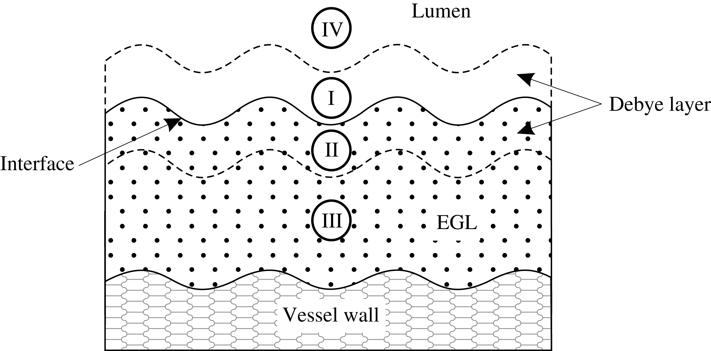
(the physiological regime, see table 1). Since this limit is singular with the small parameter multiplying the highest-order derivative, we employ from the outset matched asymptotic expansions. The asymptotic structure of the dynamics consists of an inner Debye layer region adjacent to the interface which is connected to outer bulk lumen/EGL regions (see figure 2). The outer bulk/lumen regions will still require a numerical treatment, although will be more computationally tractable than in the full problem.
Schematic representation of the near-wall region. Regions I and II correspond to the inner Debye layers in the lumen and the EGL respectively where the electric potential and ion concentrations change significantly. The characteristic thickness of each layer is of order
 $\unicode[STIX]{x1D6FF}$
. Regions III and IV are the outer regions where electroneutrality holds.
In regions III and IV we perform a small parameter expansion of the form
 $f=f^{(0)}+\unicode[STIX]{x1D6FF}^{2}f^{(1)}+\cdots \,$
for each of the variables
 $(\boldsymbol{u},\;\boldsymbol{v}_{\unicode[STIX]{x1D6FD}},\;c_{\unicode[STIX]{x1D6FD}\pm },\;\unicode[STIX]{x1D711}_{\unicode[STIX]{x1D6FD}})$
.
3.1 Electrodynamics
Keeping the zero-order terms we obtain the following system
 $$\begin{eqnarray}\displaystyle & \displaystyle \unicode[STIX]{x1D735}(c_{\unicode[STIX]{x1D6FD}+}^{(0)}+c_{\unicode[STIX]{x1D6FD}-}^{(0)})+h_{\unicode[STIX]{x1D6FD}}c_{s}\unicode[STIX]{x1D735}\unicode[STIX]{x1D711}_{\unicode[STIX]{x1D6FD}}^{(0)}=0, & \displaystyle\end{eqnarray}$$
 $$\begin{eqnarray}\displaystyle & \displaystyle \unicode[STIX]{x1D719}\unicode[STIX]{x1D735}(c_{f+}^{(0)}+c_{f-}^{(0)})-c_{s}\unicode[STIX]{x1D735}\unicode[STIX]{x1D711}_{f}^{(0)}=0, & \displaystyle\end{eqnarray}$$
 $$\begin{eqnarray}\displaystyle & \displaystyle \unicode[STIX]{x1D735}\boldsymbol{\cdot }\left[\unicode[STIX]{x1D6FE}_{\pm }c_{\unicode[STIX]{x1D6FD}\pm }^{(0)}\boldsymbol{v}^{(0)}-\unicode[STIX]{x1D735}c_{\unicode[STIX]{x1D6FD}\pm }^{(0)}\mp c_{\unicode[STIX]{x1D6FD}\pm }^{(0)}\unicode[STIX]{x1D735}\unicode[STIX]{x1D711}_{\unicode[STIX]{x1D6FD}}^{(0)}\right]=0, & \displaystyle\end{eqnarray}$$
 $$\begin{eqnarray}\displaystyle & \displaystyle c_{\unicode[STIX]{x1D6FD}+}^{(0)}-c_{\unicode[STIX]{x1D6FD}-}^{(0)}-h_{\unicode[STIX]{x1D6FD}}c_{s}=0, & \displaystyle\end{eqnarray}$$
together with flow incompressibility
 $\unicode[STIX]{x1D735}\boldsymbol{\cdot }\boldsymbol{u}_{\unicode[STIX]{x1D6FD}}^{(0)}=0$
. These zeroth-order outer equations are satisfied by constant ion concentrations and electric potential, i.e.
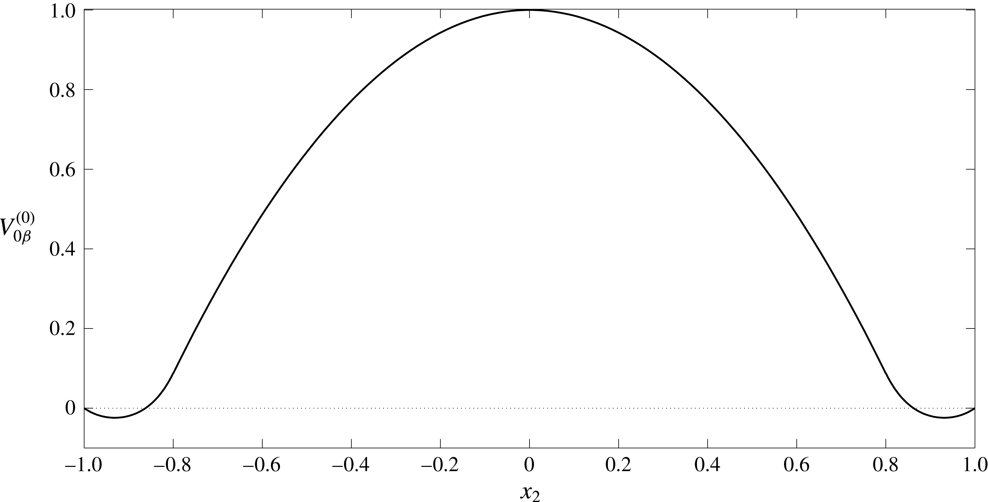
 $$\begin{eqnarray}c_{f\pm }^{(0)}=C_{f\pm }^{(0)},\quad c_{l\pm }^{(0)}=1,\quad \unicode[STIX]{x1D711}_{l}^{(0)}=0,\quad \unicode[STIX]{x1D711}_{f}^{(0)}=\unicode[STIX]{x1D6F9}_{f}^{(0)},\quad \boldsymbol{i}_{\unicode[STIX]{x1D6FD}}^{(0)}=h_{\unicode[STIX]{x1D6FD}}c_{s}\boldsymbol{v}_{\unicode[STIX]{x1D6FD}}^{(0)},\end{eqnarray}$$
where
 $C_{f+}^{(0)}-C_{f-}^{(0)}=c_{s}$
(since we have non-dimensionalised ion concentrations on their luminal values, and can set the reference potential to be zero without loss of generality). Here
 $C_{f\pm }^{(0)}$
and
 $\unicode[STIX]{x1D6F9}_{f}^{(0)}$
are currently unknown constants. Analysis of the Debye layer (see appendix B) shows us that
 $$\begin{eqnarray}\displaystyle & \displaystyle \unicode[STIX]{x1D711}_{f}^{(0)}=\operatorname{arcsinh}\left(-\frac{c_{s}}{2}\right),\quad C_{f\pm }^{(0)}=\exp \!\left(\mp \operatorname{arcsinh}\left(-\frac{c_{s}}{2}\right)\right). & \displaystyle\end{eqnarray}$$
The zero net current condition takes the form
 $$\begin{eqnarray}\displaystyle \int _{{\mathcal{S}}_{m}^{in}}\boldsymbol{v}_{f}^{(0)}\boldsymbol{\cdot }\boldsymbol{n}\,\text{d}S=0. & & \displaystyle\end{eqnarray}$$
It can be seen from (3.12) that the net fluid flux through the EGL is zero. Consequently, for a given applied pressure, the induced streaming potential leads to a reduced volumetric flow rate through the vessel.
3.2 Electro-poroelastohydrodynamics
Determining the behaviour of the flow in the bulk lumen/EGL and of the solid phase in the EGL requires us to examine (3.1)–(3.5) at
 $O(\unicode[STIX]{x1D6FF})$
:
 $$\begin{eqnarray}\displaystyle & \displaystyle \unicode[STIX]{x1D6FB}^{2}\boldsymbol{v}_{\unicode[STIX]{x1D6FD}}^{(0)}=\unicode[STIX]{x1D735}p_{\unicode[STIX]{x1D6FD}}^{(0)}+2\unicode[STIX]{x1D6FC}_{\unicode[STIX]{x1D6FD}}\unicode[STIX]{x1D735}c_{\unicode[STIX]{x1D6FD}}^{(1)}+\unicode[STIX]{x1D6FC}_{\unicode[STIX]{x1D6FD}}h_{\unicode[STIX]{x1D6FD}}c_{s}\unicode[STIX]{x1D735}\unicode[STIX]{x1D711}_{\unicode[STIX]{x1D6FD}}^{(1)}+\unicode[STIX]{x1D712}h_{\unicode[STIX]{x1D6FD}}\boldsymbol{v}_{\unicode[STIX]{x1D6FD}}^{(0)}, & \displaystyle\end{eqnarray}$$
 $$\begin{eqnarray}\displaystyle & \displaystyle \frac{1}{1-2\unicode[STIX]{x1D708}}\unicode[STIX]{x1D735}\boldsymbol{\cdot }(\unicode[STIX]{x1D735}\boldsymbol{u}^{(0)})+\unicode[STIX]{x1D6FB}^{2}\boldsymbol{u}^{(0)}=\unicode[STIX]{x1D719}\unicode[STIX]{x1D735}p_{f}^{(0)}+2\unicode[STIX]{x1D719}\unicode[STIX]{x1D6FC}_{f}\unicode[STIX]{x1D735}c_{f}^{(1)}-\unicode[STIX]{x1D6FC}_{f}c_{s}\unicode[STIX]{x1D735}\unicode[STIX]{x1D711}_{f}^{(1)}-\unicode[STIX]{x1D712}\boldsymbol{v}_{f}^{(0)}, & \displaystyle\end{eqnarray}$$
 $$\begin{eqnarray}\displaystyle & \displaystyle \unicode[STIX]{x1D6FE}_{+}\unicode[STIX]{x1D735}c_{\unicode[STIX]{x1D6FD}}^{(1)}\boldsymbol{\cdot }\boldsymbol{v}_{\unicode[STIX]{x1D6FD}}^{(0)}-\unicode[STIX]{x1D6FB}^{2}c_{\unicode[STIX]{x1D6FD}}^{(1)}-c_{\unicode[STIX]{x1D6FD}+}^{(0)}\unicode[STIX]{x1D6FB}^{2}\unicode[STIX]{x1D711}_{\unicode[STIX]{x1D6FD}}^{(1)}=0, & \displaystyle\end{eqnarray}$$
 $$\begin{eqnarray}\displaystyle & \displaystyle \unicode[STIX]{x1D6FE}_{-}\unicode[STIX]{x1D735}c_{\unicode[STIX]{x1D6FD}}^{(1)}\boldsymbol{\cdot }\boldsymbol{v}_{\unicode[STIX]{x1D6FD}}^{(0)}-\unicode[STIX]{x1D6FB}^{2}c_{\unicode[STIX]{x1D6FD}}^{(1)}+c_{\unicode[STIX]{x1D6FD}-}^{(0)}\unicode[STIX]{x1D6FB}^{2}\unicode[STIX]{x1D711}_{\unicode[STIX]{x1D6FD}}^{(1)}=0, & \displaystyle\end{eqnarray}$$
 $$\begin{eqnarray}\displaystyle & \displaystyle c_{\unicode[STIX]{x1D6FD}+}^{(1)}=c_{\unicode[STIX]{x1D6FD}-}^{(1)}=c_{\unicode[STIX]{x1D6FD}}^{(1)}. & \displaystyle\end{eqnarray}$$
After adding and subtracting (3.15) with (3.16) and using (3.17) we come to the following reduced form
 $$\begin{eqnarray}\displaystyle & \displaystyle \unicode[STIX]{x1D6FB}^{2}\boldsymbol{v}_{\unicode[STIX]{x1D6FD}}^{(0)}=\unicode[STIX]{x1D735}p_{\unicode[STIX]{x1D6FD}}^{(0)}+2\unicode[STIX]{x1D6FC}_{\unicode[STIX]{x1D6FD}}\unicode[STIX]{x1D735}c^{(1)}+\unicode[STIX]{x1D6FC}_{\unicode[STIX]{x1D6FD}}h_{\unicode[STIX]{x1D6FD}}c_{s}\unicode[STIX]{x1D735}\unicode[STIX]{x1D711}_{\unicode[STIX]{x1D6FD}}^{(1)}+\unicode[STIX]{x1D712}h_{\unicode[STIX]{x1D6FD}}\boldsymbol{v}_{\unicode[STIX]{x1D6FD}}^{(0)}, & \displaystyle\end{eqnarray}$$
 $$\begin{eqnarray}\displaystyle & \displaystyle \frac{1}{1-2\unicode[STIX]{x1D708}}\unicode[STIX]{x1D735}\boldsymbol{\cdot }(\unicode[STIX]{x1D735}\boldsymbol{u}^{(0)})+\unicode[STIX]{x1D6FB}^{2}\boldsymbol{u}^{(0)}=\unicode[STIX]{x1D719}\unicode[STIX]{x1D735}p_{f}^{(0)}+2\unicode[STIX]{x1D719}\unicode[STIX]{x1D6FC}\unicode[STIX]{x1D735}c_{f}^{(1)}-\unicode[STIX]{x1D6FC}c_{s}\unicode[STIX]{x1D735}\unicode[STIX]{x1D711}_{f}^{(1)}-\unicode[STIX]{x1D712}\boldsymbol{v}_{f}^{(0)}, & \displaystyle\end{eqnarray}$$
 $$\begin{eqnarray}\displaystyle & \displaystyle (\unicode[STIX]{x1D6FE}_{+}+\unicode[STIX]{x1D6FE}_{-})\unicode[STIX]{x1D735}c_{\unicode[STIX]{x1D6FD}}^{(1)}\boldsymbol{\cdot }\boldsymbol{v}_{\unicode[STIX]{x1D6FD}}^{(0)}-2\unicode[STIX]{x1D6FB}^{2}c_{\unicode[STIX]{x1D6FD}}^{(1)}-h_{\unicode[STIX]{x1D6FD}}c_{s}\unicode[STIX]{x1D6FB}^{2}\unicode[STIX]{x1D711}_{\unicode[STIX]{x1D6FD}}^{(1)}=0, & \displaystyle\end{eqnarray}$$
 $$\begin{eqnarray}\displaystyle & \displaystyle (\unicode[STIX]{x1D6FE}_{+}-\unicode[STIX]{x1D6FE}_{-})\unicode[STIX]{x1D735}c_{\unicode[STIX]{x1D6FD}}^{(1)}\boldsymbol{\cdot }\boldsymbol{v}_{\unicode[STIX]{x1D6FD}}^{(0)}-c_{\unicode[STIX]{x1D6FD}}^{(0)}\unicode[STIX]{x1D6FB}^{2}\unicode[STIX]{x1D711}_{\unicode[STIX]{x1D6FD}}^{(1)}=0, & \displaystyle\end{eqnarray}$$
where
 $c_{l}^{(0)}=(c_{l+}^{(0)}+c_{l-}^{(0)})=2$
and
 $c_{f}^{(0)}=(c_{f+}^{(0)}+c_{f-}^{(0)})=2\cosh (\operatorname{arcsinh}(-c_{s}/2))$
.
It proves convenient to express the potentials and ion concentrations as the sum of two components: homogeneous solutions
 $\unicode[STIX]{x1D711}_{\unicode[STIX]{x1D6FD}h}^{(1)}$
,
 $c_{\unicode[STIX]{x1D6FD}h}^{(1)}$
that satisfy inlet/outlet conditions but which is continuous across the EGL–lumen interface, and non-homogeneous solutions
 $\unicode[STIX]{x1D711}_{\unicode[STIX]{x1D6FD}p}^{(1)}$
,
 $c_{\unicode[STIX]{x1D6FD}p}^{(1)}$
that satisfy the jump conditions across the Debye layer (as determined by the analysis in appendix B), e.g.
 $$\begin{eqnarray}\displaystyle c_{\unicode[STIX]{x1D6FD}}^{(1)} & = & \displaystyle c_{\unicode[STIX]{x1D6FD}h}^{(1)}+c_{\unicode[STIX]{x1D6FD}p}^{(1)},\quad \unicode[STIX]{x1D711}_{\unicode[STIX]{x1D6FD}}^{(1)}=\unicode[STIX]{x1D711}_{\unicode[STIX]{x1D6FD}h}^{(1)}+\unicode[STIX]{x1D711}_{\unicode[STIX]{x1D6FD}p}^{(1)}.\end{eqnarray}$$
The first-order corrections (3.18)–(3.21) are subject to the following boundary conditions on the solid walls
 $$\begin{eqnarray}\displaystyle \frac{\unicode[STIX]{x2202}c_{\unicode[STIX]{x1D6FD}h}^{(1)}}{\unicode[STIX]{x2202}n} & = & \displaystyle \frac{\unicode[STIX]{x2202}c_{\unicode[STIX]{x1D6FD}p}^{(1)}}{\unicode[STIX]{x2202}n}=0,\quad \frac{\unicode[STIX]{x2202}\unicode[STIX]{x1D711}_{\unicode[STIX]{x1D6FD}h}^{(1)}}{\unicode[STIX]{x2202}n}=\frac{\unicode[STIX]{x2202}\unicode[STIX]{x1D711}_{\unicode[STIX]{x1D6FD}p}^{(1)}}{\unicode[STIX]{x2202}n}=0,\end{eqnarray}$$
and at the inlet/outlet
 $$\begin{eqnarray}\boldsymbol{v}_{\unicode[STIX]{x1D6FD}}^{(0)}=\boldsymbol{{\mathcal{V}}}_{\unicode[STIX]{x1D6FD}}^{(0)},\quad \boldsymbol{u}^{(0)}=\boldsymbol{{\mathcal{U}}}^{(0)},\quad c_{\unicode[STIX]{x1D6FD}h}^{(1)}={\mathcal{C}}_{\unicode[STIX]{x1D6FD}}^{(1)},\quad c_{\unicode[STIX]{x1D6FD}p}^{(1)}=0,\quad \unicode[STIX]{x1D711}_{\unicode[STIX]{x1D6FD}h}^{(1)}=\unicode[STIX]{x1D6F7}_{\unicode[STIX]{x1D6FD}}^{(1)},\quad \unicode[STIX]{x1D711}_{\unicode[STIX]{x1D6FD}p}^{(1)}=0,\end{eqnarray}$$
where the constants
 $\boldsymbol{{\mathcal{V}}}_{\unicode[STIX]{x1D6FD}}^{(0)}$
,
 $\boldsymbol{{\mathcal{U}}}^{(0)}$
,
 ${\mathcal{C}}_{\unicode[STIX]{x1D6FD}}^{(1)}(=0)$
and
 $\unicode[STIX]{x1D6F7}_{\unicode[STIX]{x1D6FD}}^{(1)}(=Bx_{1})$
are given in appendix A.
To close the model we need to specify boundary conditions at the lumen–EGL interface. These are determined by the Debye layer (inner solution) that straddles the lumen–EGL interface, and across which we expect potential and ion concentrations to vary rapidly. This analysis, details of which can be found in appendix B, tell us that at the interface
 $$\begin{eqnarray}\displaystyle & & \displaystyle \displaystyle c_{lh}^{(1)}=c_{fh}^{(1)},\quad \unicode[STIX]{x1D711}_{lh}^{(1)}=\unicode[STIX]{x1D711}_{fh}^{(1)},\end{eqnarray}$$
and
 $$\begin{eqnarray}\displaystyle & \displaystyle c_{\unicode[STIX]{x1D6FD}p}^{(1)}=-A_{\unicode[STIX]{x1D6FD}c}\frac{\unicode[STIX]{x2202}(\boldsymbol{v}_{\unicode[STIX]{x1D6FD}}^{(0)}\boldsymbol{\cdot }\unicode[STIX]{x1D749})}{\unicode[STIX]{x2202}\unicode[STIX]{x1D70F}}, & \displaystyle\end{eqnarray}$$
 $$\begin{eqnarray}\displaystyle & \displaystyle \unicode[STIX]{x1D711}_{\unicode[STIX]{x1D6FD}p}^{(1)}=-A_{\unicode[STIX]{x1D6FD}\unicode[STIX]{x1D711}}\frac{\unicode[STIX]{x2202}(\boldsymbol{v}_{\unicode[STIX]{x1D6FD}}^{(0)}\boldsymbol{\cdot }\unicode[STIX]{x1D749})}{\unicode[STIX]{x2202}\unicode[STIX]{x1D70F}}, & \displaystyle\end{eqnarray}$$
where
 $\unicode[STIX]{x1D749}$
is a local tangent vector and the coefficients
 $A_{\unicode[STIX]{x1D6FD}c}$
and
 $A_{\unicode[STIX]{x1D6FD}\unicode[STIX]{x1D711}}$
are found numerically (see (B 45)). Flow boundary conditions on the interface are
 $$\begin{eqnarray}\displaystyle & \displaystyle \boldsymbol{v}_{l}^{(0)}=\unicode[STIX]{x1D719}_{f}\boldsymbol{v}_{f}^{(0)},\quad \unicode[STIX]{x1D748}_{l}^{(0)}\boldsymbol{\cdot }\boldsymbol{n}=\unicode[STIX]{x1D748}_{f}^{(0)}\boldsymbol{\cdot }\boldsymbol{n}-A_{p}\frac{\unicode[STIX]{x2202}(\boldsymbol{v}_{f}^{(0)}\boldsymbol{\cdot }\unicode[STIX]{x1D749})}{\unicode[STIX]{x2202}\unicode[STIX]{x1D70F}}\boldsymbol{n}. & \displaystyle\end{eqnarray}$$
For the solid phase the relationship between tractions on the interface is given by
 $$\begin{eqnarray}\displaystyle \unicode[STIX]{x1D719}\unicode[STIX]{x1D748}_{l}^{(0)}\boldsymbol{\cdot }\boldsymbol{n} & = & \displaystyle \unicode[STIX]{x1D748}_{s}^{(0)}\boldsymbol{\cdot }\boldsymbol{n}-\unicode[STIX]{x1D719}A_{p}\frac{\unicode[STIX]{x2202}(\boldsymbol{v}_{f}^{(0)}\boldsymbol{\cdot }\unicode[STIX]{x1D749})}{\unicode[STIX]{x2202}\unicode[STIX]{x1D70F}}\boldsymbol{n}.\end{eqnarray}$$
The coefficient
 $A_{p}$
is also found numerically (see (B 47)). With the boundary and interface conditions now specified, the reduced model (3.18)–(3.21) for the bulk domain can be solved.
Let us consider first the homogeneous solutions for ion concentrations and potential. The zero inlet values of ion concentration (3.24) and zero flux conditions across the vessel walls (3.24) both suggest homogeneous solutions that satisfy
 $$\begin{eqnarray}\displaystyle & \displaystyle c_{lh}^{(1)}=c_{fh}^{(1)}=0, & \displaystyle\end{eqnarray}$$
 $$\begin{eqnarray}\displaystyle & \displaystyle \unicode[STIX]{x1D6FB}^{2}\unicode[STIX]{x1D711}_{\unicode[STIX]{x1D6FD}h}^{(1)}=0, & \displaystyle\end{eqnarray}$$
where
 $\unicode[STIX]{x2202}\unicode[STIX]{x1D711}_{\unicode[STIX]{x1D6FD}h}^{(1)}/\unicode[STIX]{x2202}n=0$
on the solid vessel walls, and
 $\unicode[STIX]{x1D711}_{\unicode[STIX]{x1D6FD}h}^{(1)}$
is continuous at the lumen/EGL interface. The inlet and outlet conditions (3.24) give
 $\unicode[STIX]{x2202}\unicode[STIX]{x1D711}_{\unicode[STIX]{x1D6FD}h}^{(1)}/\unicode[STIX]{x2202}n=B$
(where B is a constant determined by the zero net current conditions (3.12)). By numerically solving (3.31) subject to these boundary conditions (see § 4 below) we obtain the streaming potential distribution.
Next we consider flow and non-homogeneous components of ion concentration and potential, driven by the Debye layer. These remain governed by (3.18)–(3.21), and the boundary conditions on the interface take the form given in (3.26)–(3.29). On the solid vessel walls we have
 $$\begin{eqnarray}\frac{\unicode[STIX]{x2202}c_{fp}^{(1)}}{\unicode[STIX]{x2202}n}=0,\quad \frac{\unicode[STIX]{x2202}\unicode[STIX]{x1D711}_{fp}^{(1)}}{\unicode[STIX]{x2202}n}=0,\quad \boldsymbol{v}_{f}^{(0)}=\boldsymbol{u}^{(0)}=0,\end{eqnarray}$$
and at the inlet/outlet
 $$\begin{eqnarray}\frac{\unicode[STIX]{x2202}\unicode[STIX]{x1D711}_{lp}^{(1)}}{\unicode[STIX]{x2202}n}=\frac{\unicode[STIX]{x2202}\unicode[STIX]{x1D711}_{fp}^{(1)}}{\unicode[STIX]{x2202}n}=0,\quad c_{lp}^{(1)}=c_{fp}^{(1)}=0,\quad \boldsymbol{v}_{\unicode[STIX]{x1D6FD}}^{(0)}=\boldsymbol{{\mathcal{V}}}_{\unicode[STIX]{x1D6FD}}^{(0)},\quad \boldsymbol{u}^{(0)}=\boldsymbol{{\mathcal{U}}}^{(0)}.\end{eqnarray}$$
Solving this system also requires a numerical approach, which we describe in the next section.
An example of the triangular mesh used in the boundary–finite element method numerical scheme to solve the dynamics in the bulk EGL/lumen.

4 Numerical methods
A coupled boundary–finite element method scheme (BEM-FEM) is used to solve numerically the first-order problem in the bulk EGL/lumen (3.31)–(3.33). This, in turn, allows us to determine the fluid and solid stresses exerted by the EGL upon the vessel wall. We note that the fluid phase (3.18) decouples from the solid phase (3.19), which allows us to solve the flow equations independently of the solid phase (but not of the ion concentrations, which provide a fluid forcing). The linearity of the governing equations for the fluid and solid phases, as well as for the homogeneous potential (3.31), allows us to take advantage of boundary integral representations, which means that we need only compute unknown fluid and elastic tractions, velocities, elastic displacements and electric potentials on the vessel boundaries (see Sumets et al. Reference Sumets, Cater, Long and Clarke2015 for more details). This is done through implementation of a boundary element method (BEM) numerical scheme which solves for these unknowns on discrete linear elements that approximate the contours of the vessel boundaries and interfaces.
The ion transport equations (3.20), (3.21), on the other hand, are nonlinear, and are solved throughout the vessel volume using a finite element method approach. This is achieved by discretising the vessel domain into a triangular mesh. Mesh refinement is applied near the interface region and within the EGL, where we might expect steep concentration gradients (see figure 3 for an example mesh). Linear interpolants for ion concentrations and potentials are used within these elements, and triangle edges on vessel boundaries are shared by both the BEM and FEM schemes. This triangular volume discretisation then allows us to convert a weak formulation of ion transport equations into a nonlinear algebraic system in the usual manner for a finite element method approach. (Note that the required values of electric potential at points within the bulk lumen and EGL can be computed a posteriori given their boundary values, again using a boundary integral representation of Laplace’s equation (3.31).)
Since the governing equations for flows, ion concentrations and potential are coupled, the FEM and BEM schemes must be solved at the same time. The resulting system of nonlinear algebraic equations is solved using MATLAB’s fsolve iterative routine. To improve numerical efficiency, the Jacobian is calculated analytically and provided to the solver. Each simulation requires approximately 180 Gb of memory and 2304 CPU hours. The calculation of the matrix coefficients was parallelised across 12 CPU cores using MATLAB’s Parallel Toolbox. As a result, each simulation takes approximately 192 hours to complete.
Convergence of the calculations was verified by a mesh refinement study, by decreasing triangle edge lengths,
 $d$
. Simulations using triangles within the EGL with a maximum edge length
 $d=0.04$
,
 $0.03$
,
 $0.02$
and
 $0.015$
demonstrated good convergence by
 $d=0.02$
. The accuracy of the scheme was also verified by simulating results for a straight-walled channel for which an analytical solution is known (see appendix A).
5 Results
We present results for numerical simulations of the electro-poroelastohydrodynamics of a microvessel coated with charged EGL. Following the earlier work that has considered a non-charged EGL (Wei et al. Reference Wei, Waters, Liu and Grotberg2003; Sumets et al. Reference Sumets, Cater, Long and Clarke2015; Lee et al. Reference Lee, Long and Clarke2016), the vessel is modelled as a two-dimensional wavy-walled channel with top and bottom walls prescribed by
 $$\begin{eqnarray}\displaystyle {\mathcal{S}} & =\left\{\begin{array}{@{}ll@{}}\pm 1,\quad & \quad -1-\frac{1}{4}\unicode[STIX]{x1D6EC}_{e}\leqslant x_{1}<-\frac{1}{4}\unicode[STIX]{x1D6EC}_{e},\\ \unicode[STIX]{x1D702}_{\pm }(x_{1}),\quad & \quad -\frac{1}{4}\unicode[STIX]{x1D6EC}_{e}\leqslant x_{1}<-\frac{1}{8}\unicode[STIX]{x1D6EC}_{e},\\ \pm 1\mp a\cos (2\unicode[STIX]{x03C0}x_{1}/\unicode[STIX]{x1D6EC}_{e}),\quad & \quad -\frac{1}{8}\unicode[STIX]{x1D6EC}_{e}\leqslant x_{1}<\frac{1}{8}\unicode[STIX]{x1D6EC}_{e},\\ \unicode[STIX]{x1D701}_{\pm }(x_{1}),\quad & \quad \frac{1}{8}\unicode[STIX]{x1D6EC}_{e}\leqslant x_{1}<\frac{1}{4}\unicode[STIX]{x1D6EC}_{e},\\ \pm 1,\quad & \quad \frac{1}{4}\unicode[STIX]{x1D6EC}_{e}\leqslant x_{1}\leqslant 1+\frac{1}{4}\unicode[STIX]{x1D6EC}_{e},\end{array}\right. & \displaystyle\end{eqnarray}$$
where the upper and lower signs correspond to upper and lower vessel walls, respectively. The functions
 $\unicode[STIX]{x1D702}_{\pm }(x_{1}),\unicode[STIX]{x1D701}_{\pm }(x_{1})$
are spline interpolations that guarantee a smooth transition from straight inlet/outlets (where the analytical solution in known, see appendix A), to the non-uniform wavy topology. In non-dimensional form, the geometry of the vessel is characterised by the mean width of
 $2$
, wall undulations of amplitude
 $a$
and wavelength
 $\unicode[STIX]{x1D6EC}_{e}$
. The EGL follows the topology of the vessel walls and has a thickness denoted by
 $\unicode[STIX]{x1D700}$
.
In what follows we examine the impact of the EGL thickness upon the fluid and solid shear stresses exerted on the vessel wall, and compare results (obtained using triphasic mixture theory) with solutions obtained for comparable uncharged EGLs (obtained using biphasic mixture theory), to gauge the influence of the EGL’s charge upon effects such as mechanotransduction. Table 2 summarises the values for the non-dimensional parameters used across the simulations based upon the physiological values of the dimensional parameters given in table 1. These include endothelial wall wavelength
 $\unicode[STIX]{x1D6EC}_{e}$
and amplitude
 $a$
, EGL permeability
 $\unicode[STIX]{x1D712}$
, EGL fixed charge
 $c_{s}$
, solid volume fraction
 $\unicode[STIX]{x1D719}_{s}$
, Poisson ratio
 $\unicode[STIX]{x1D708}$
, Péclet number for the cations (anions)
 $c_{+}$
(
 $c_{-}$
), ion-drag coefficient
 $\unicode[STIX]{x1D6FC}_{l}$
. The magnitudes of wall amplitude and wavelength are chosen to reflect the restrictions on curvature discussed in appendix B.
Non-dimensional parameter values for a capillary lined with a charged EGL.

We consider four cases corresponding to different combinations of the EGL thickness and presence of charge effects (see table 3 for a summary showing fixed charge concentration
 $c_{s}$
which determines whether the charge effect is considered, and EGL thickness,
 $\unicode[STIX]{x1D700}$
). Accordingly, Cases A and B correspond to the charged EGL with thicknesses
 $\unicode[STIX]{x1D700}=0.2$
(Case A) and
 $\unicode[STIX]{x1D700}=0.1$
(Case B). Cases C and D consider the EGL without charge and with thicknesses
 $\unicode[STIX]{x1D700}=0.2$
(Case C) and
 $\unicode[STIX]{x1D700}=0.1$
(Case D). In what follows we present flow fields and associated shear stresses,
 $\unicode[STIX]{x1D6E4}_{f}$
and
 $\unicode[STIX]{x1D6E4}_{s}$
on the vessel walls and elastic displacements in the EGL corresponding to these geometries.
Flow field in the region of the EGL for Case A, showing reversed flow near to the vessel wall.

Parameters for the various cases considered.

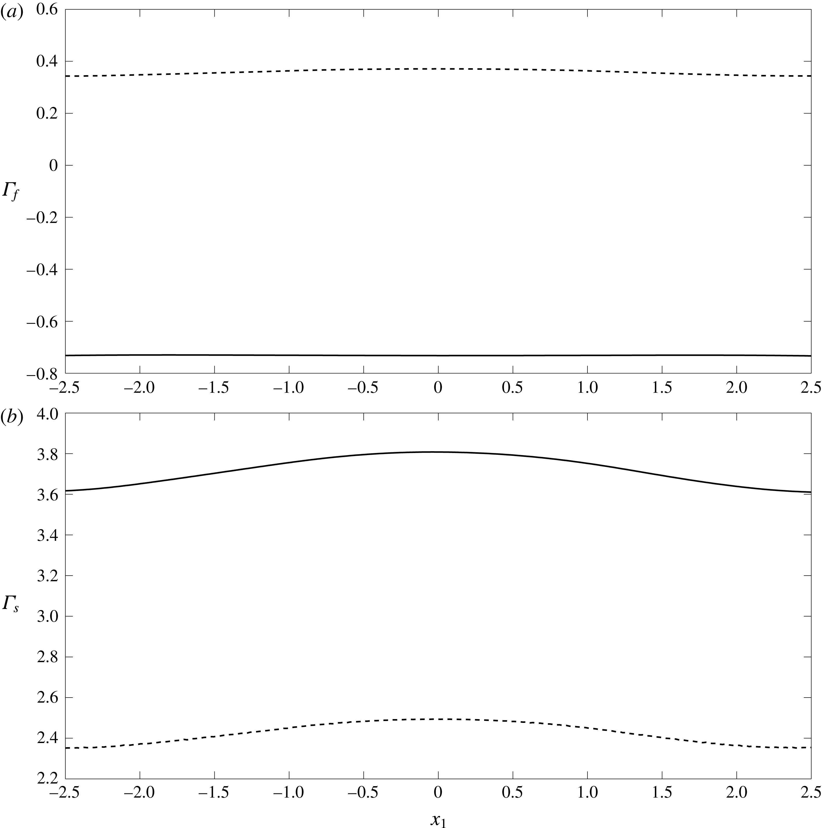
Comparison of the fluid
 $\unicode[STIX]{x1D6E4}_{f}$
(
 $a$
) and elastic
 $\unicode[STIX]{x1D6E4}_{s}$
(
 $b$
) shear stresses on a vessel wall with EGL thickness
 $\unicode[STIX]{x1D700}=0.2$
. The solid lines (——) are the predictions made in the presence of charge effects (TMT solutions, Case A) and the dashed lines (- - - -) are those made in the absence of charge effects (BMT solutions, Case C).
The near-wall flow field for the vessel when the EGL thickness is
 $\unicode[STIX]{x1D716}=0.2$
(Case A) is examined in figure 4. These have been found by solving the governing equations in the bulk EGL/lumen (3.18)–(3.21) using the BEM-FEM numerical scheme described in § 4. One significant observation is that the flow is reversed near the vessel wall, which does not occur in the absence of charge effects (Sumets et al.
Reference Sumets, Cater, Long and Clarke2015; Lee et al.
Reference Lee, Long and Clarke2016). As expected, this leads to a reversal of the fluid shear stresses exerted upon the vessel wall, as shown in figure 5. We also see that the presence of charge effects (under otherwise identical conditions) is associated with a higher magnitude fluid shear stresses and elastic stresses. We also note that the magnitude of the solid shear stress is approximately ten times greater than the magnitude of the shear stress due to the fluid phase. This is an effect that has been previously noted in the absence of EGL charge (Sumets et al.
Reference Sumets, Cater, Long and Clarke2015; Lee et al.
Reference Lee, Long and Clarke2016) and suggests that much of the applied mechanical load is carried through the solid rather than fluid phase of the EGL. We also note the effect of wall topology on the stress profiles. We see that the
 $2\,\%$
variation in wall location leads to an associated
 $5{-}6\,\%$
variation in solid stresses irrespective of whether or not charge effects are present (figure 5
b). We see a similar sensitivity to topology in the fluid stresses in the absence of charge effects, although this sensitivity of fluid stress to wall shape appears to be dampened when charge effects are present (figure 5
a).
We also investigate the influence of EGL thickness on the stresses exerted on the solid wall. Figures 6 and 7 compare the elastic and fluid stress distributions in Cases A–D when
 $\unicode[STIX]{x1D700}=0.1$
and
 $\unicode[STIX]{x1D700}=0.2$
. In figure 6(
 $b$
) it is seen that a reduction in EGL thickness leads to a non-proportional reduction in the elastic stresses exerted upon the wall. Fluid shear stresses are negative and increase in magnitude by approximately
 $30\,\%$
with reduced layer thickness. Hence, we observe increased magnitude
 $\unicode[STIX]{x1D6E4}_{f}$
and decreased magnitude
 $\unicode[STIX]{x1D6E4}_{s}$
when the EGL thickness is reduced twofold. We also again observe that solid stresses appear to be more sensitive to wall topology than fluid stresses, when charge effects are present, and that this sensitivity does not appear to change greatly when the thickness of the EGL is doubled. Another observation following from figure 7 is that for thin EGL the magnitudes of fluid shear stresses are largely the same regardless of charge effects (although there is still a sign change) while the shear stress due to the solid phase with the presence of charge takes higher value relative to charge-free case. We again see for this thinner EGL how the presence of charge tends to reduce the sensitivity of the fluid stress to wall shape.
Comparison of the fluid
 $\unicode[STIX]{x1D6E4}_{f}$
(
 $a$
) and elastic
 $\unicode[STIX]{x1D6E4}_{s}$
(
 $b$
) shear stresses on the vessel wall. Here the solid lines correspond to Case A (typical EGL thickness
 $\unicode[STIX]{x1D700}=0.2$
) and the dashed lines to Case B (thin EGL thickness
 $\unicode[STIX]{x1D700}=0.1$
).

Comparison of the fluid
 $\unicode[STIX]{x1D6E4}_{f}$
(
 $a$
) and elastic
 $\unicode[STIX]{x1D6E4}_{s}$
(
 $b$
) shear stresses on the vessel wall for thin EGL (thickness
 $\unicode[STIX]{x1D700}=0.1$
). Here the solid lines correspond to Case B (with charge) and the dashed lines to Case D (charge free).
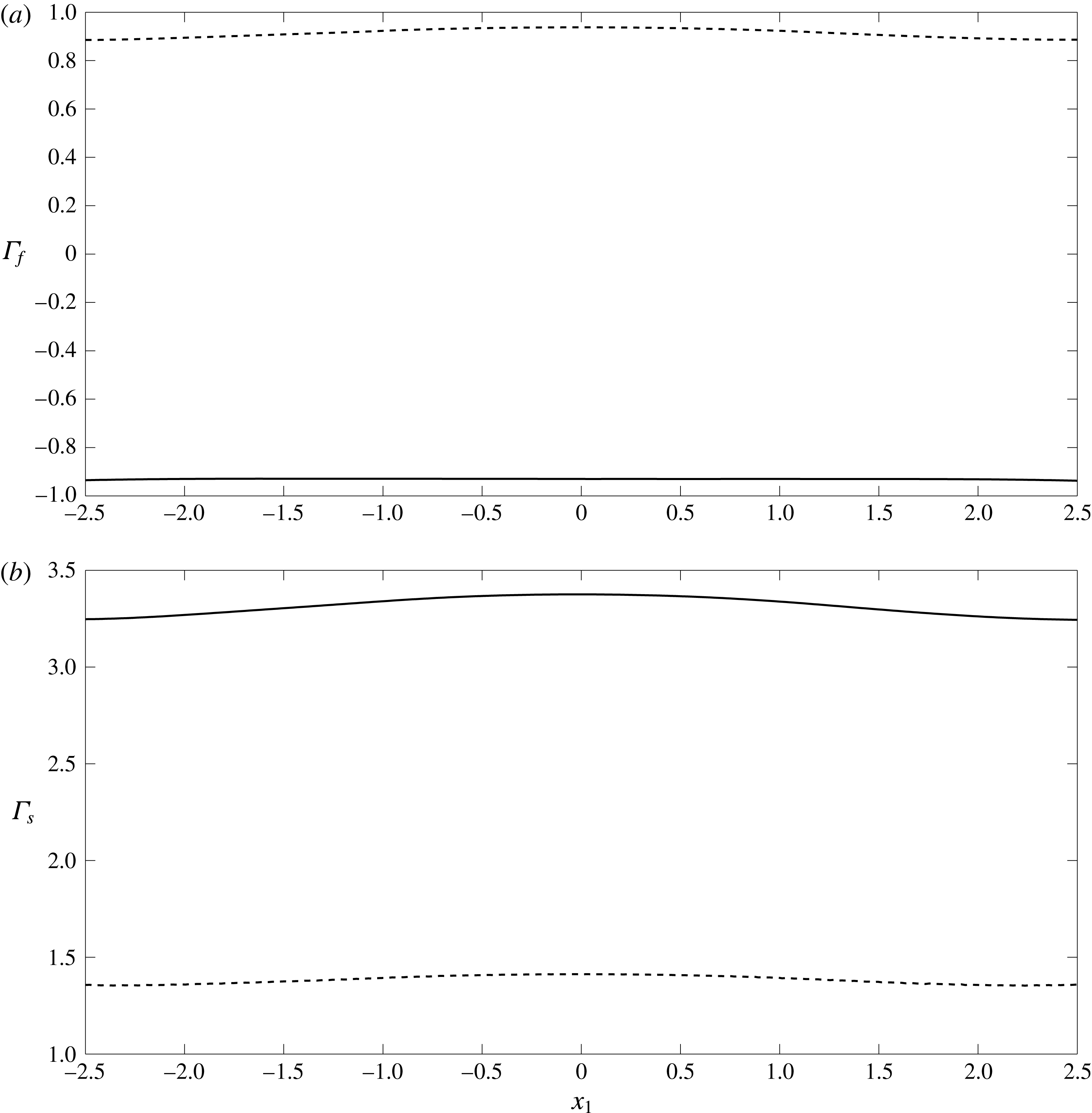
If we examine the ion concentration gradients throughout the vessel, as shown in figure 8, we see that the spatial variations at the wall persist largely unaltered throughout the thickness of EGL, before undergoing a jump at the EGL/lumen interface as mediated by the (here, asymptotically thin) Debye layer. It is also evident that the variations in ion concentrations in the lumen are very small compared with the variations seen within the EGL (since at leading order the ion concentrations in both lumen and EGL are spatially constant; recall that these ion concentration predictions were made under the assumption that steric interactions are negligible. This will generally cease to be the case when
 $c_{max}^{\ast }\sim 1/{a^{\ast }}^{3}$
where
 $a^{\ast }\approx 2\times 10^{-10}~\text{m}$
is the ionic radius (Kilic & Bazant Reference Kilic and Bazant2007). This corresponds to non-dimensional ion concentrations
 $c\sim 10^{4}$
, which is well above those seen here.)
Ion concentration
 $c^{(1)}$
for Case A.

6 Discussion
In this study we have investigated the influence of the endothelial glycocalyx layer’s (EGL) negative charge upon microvessel hemodynamics. We have used a triphasic mixture theory (TMT) model, which couples together governing equations for the fluid flow, elastic deformations of the EGL, transport of dissolved ions and any electric fields that are established as a result. We found that the combined presence of a negatively charged EGL and a pressure-driven flow through the microvessel can create gradients in the concentrations of charged ions in the blood plasma (such as sodium and chloride), as well as associated electric fields. Although these gradients are small in this microvessel (scaling like the Debye layer thickness) we have shown that they still couple strongly into the governing flow and elasticity equations, and hence can have a significant influence upon the flow and elastic deformations of the EGL. This extends previous theoretical studies of the EGL which have either neglected charge effects altogether (Damiano et al. Reference Damiano, Duling, Ley and Skalak1996; Wei et al. Reference Wei, Waters, Liu and Grotberg2003; Sumets et al. Reference Sumets, Cater, Long and Clarke2015; Lee et al. Reference Lee, Long and Clarke2016), or considered only drainage flows generated by the motion of the EGL’s solid matrix under crushing and subsequent elastic relaxation (e.g. no pressure-driven flow through the microvessel). The latter leads to electroneutrality, and ion concentrations that assume a classical Boltzmann spatial distribution (Damiano & Stace Reference Damiano and Stace2002).
By contrast, we have found here that in the thin Debye layer which straddles the EGL/lumen interface electroneutrality is locally broken, and that across the layer there is a rapid variation in the values of ion concentrations and electric potential. This layer is difficult to resolve numerically, but does lend itself to an asymptotic treatment. The resulting analysis provided us with effective jump conditions across the EGL/lumen, which we can then use to perform full boundary–finite element method computations in the bulk EGL/lumen. Using this computational scheme we have been able to explore the effect of the EGL thickness upon the poroelastic dynamics of the EGL, and compare these results with those obtained in the absence of any charge effects (obtained using biphasic mixture theory, which neglects the ionic phase and electric potential).
Some of the main results found in the absence of charge effects persist, for example, the dominance of solid stress over fluid stress (Secomb, Hsu & Pries Reference Secomb, Hsu and Pries2001), as well as the increase (decrease) in solid (fluid) stress as the EGL becomes thicker. However, quantitative comparison shows that the proportion of the solid shear stress in the total stress in the presence of charge effects is 90 % which is slightly higher than that when charge effects are absent (85 %). With a layer of double the thickness, the solid stress increases by 45 % in the absence of charge effects, whereas the solid stress increases by only 20 % with charge effects present. This suggests that the presence of charge might render mechanotransduction through the EGL less sensitive to reduction in its thickness, which could be clinically important in the context of the EGL remaining effective under degradation through injury or disease.
The most striking difference that occurs when charge effects are included is the appearance of reversed flow in the EGL, which leads to negative fluid shear stress along the length of the vessel wall. This happens because a streaming potential is created in the EGL which exerts an opposing body force on the fluid. In the absence of charge effects, negative fluid shear only seems to appear in the presence of a localised viscous eddy (Wei et al. Reference Wei, Waters, Liu and Grotberg2003; Sumets et al. Reference Sumets, Cater, Long and Clarke2015). This could be important because fluid shear stress affects the endothelial cells in different ways from the stresses carried through the EGL’s solid matrix (Weinbaum et al. Reference Weinbaum, Tarbell and Damiano2007), and could therefore have significant implications for phenomena such as mechanotransduction in the microvasculature. For example, these findings suggest that changes in ion concentrations in the plasma, or compromised EGL charge (resulting from a disease state, damage, or altered blood chemistry) could influence transmission of mechanical information to the underlying endothelial cells, and hence potentially endothelial remodelling under fluid shear. We have also observed that the presence of charge effects seem to reduce the sensitivity of the fluid shear stresses to the variations in wall geometry. By contrast, the solid stresses appear to have a spatial profile which mirror the variations in wall geometry irrespective of whether or not charge effects are included.
We note that there are a number of effects that have not been included in this study. We have considered only small elastic deformations of the EGL, which precludes crushing of the layer by passing white blood cells. Such a situation would be of interest in the context of the body’s immune response, where leukocytes must penetrate sufficiently deep into the EGL to bind to sites of damage or inflammation. Large scale deformations can be associated with changes in the EGL’s solid volume fraction, and lead to more acute variations in ion concentration gradients and electric potential (Damiano & Stace Reference Damiano and Stace2002). There is an interesting debate around whether osmotic pressures set up by these gradients, or the intrinsic elasticity of the EGL, plays the greater role in restoring the EGL to its undeformed state (Secomb, Hsu & Pries Reference Secomb, Hsu and Pries1998). We are not in a position to inform that debate here, however, our study suggests that the coupling of the background flow with the electrochemistry could be an important factor to consider when attempting to address this question.
We have also assumed that the EGL behaves like an homogeneous, isotropic porous material. Its actual physical structure is far more complex, and the subject of ongoing experimental research (Squire et al. Reference Squire, Chew, Nneji, Neal, Barry and Michel2001; Arkill et al. Reference Arkill, Neal, Mantell, Michel, Qvortrup, Rostgaard, Bates, Knupp and Squire2012). Some relatively recent evidence suggests that the EGL’s microstructure consists of a periodic array of core proteins of length 150–400 nm, spaced at 20 nm (Squire et al. Reference Squire, Chew, Nneji, Neal, Barry and Michel2001). It seems reasonable that such an organisational structure at the microscopic level could lead to anisotropy in the bulk behaviour at the macroscopic level. Porous models where the bulk permeability has been obtained through homogenisation might be one way to incorporate such details. We should also note that we have modelled the mechanics within the Debye layer using continuum equations, in spite of its very small physical thickness. This might be an assumption that deserves further scrutiny in the future. We have also considered a regime where the curvature is small compared to the Debye layer thickness. While this is sufficient to highlight the importance of electroviscous effects, the analysis could be extended to consider arbitrary curvatures by following the approach of Cox (Reference Cox1997) and Yariv et al. (Reference Yariv, Schnitzer and Frankel2011) (although this does increase the complexity of the analysis considerably). In case of slowly varying vessel geometries, it is perhaps also worth mentioning that a long-wavelength asymptotic approach (cf. Wei et al. Reference Wei, Waters, Liu and Grotberg2003) might also be a convenient alternative to full numerical computation.
Furthermore, the vessel wall has been treated as an impermeable barrier. In fact, transmural flows can be important, for example, in the formation of lipid-rich plaques on microvessel walls as a precursor to conditions like atherosclerosis (Vincent, Sherwin & Weinberg Reference Vincent, Sherwin and Weinberg2010). Such transmural flows can also lead to transport of ions across between the endothelium and the vessel lumen/EGL (Sawyer & Stanczewski Reference Sawyer, Stanczewski, Effert and Meyer-Erkelenz1976), which could potentially lead to small electrical currents being generated along the vessel. This, in turn, could affect the generated streaming potential and consequently the magnitude of the reversed flow effects reported in this study, and so could warrant future inclusion in the analysis. There has also been some recent theoretical work which models the EGL as an array of charged cylinders and suggests that the transmural transport of charged solutes might be significantly affected by the EGL’s charge. Therefore, it could prove valuable to include transmural flow through the clefts between endothelial cells into this charged EGL model.
Acknowledgements
P.P.S. is funded by a University of Auckland Doctoral Scholarship. The authors wish to acknowledge the contribution of NeSI high-performance computing facilities to the results of this research. New Zealands national facilities are provided by the NZ eScience Infrastructure and funded jointly by NeSIs collaborator institutions and through the Ministry of Business, Innovation & Employments Research Infrastructure programme, URL https://www.nesi.org.nz. The authors would also like to thank Dr B. Ruddy, Professor P. Hunter and A/Professor A. Taberner for some useful conversations around electroviscous effects in blood vessels.
Appendix A. Zero-order flow for the straight-walled vessel
We seek a solution for the fully developed straight-walled problem in the form
 $$\begin{eqnarray}\displaystyle & \displaystyle \boldsymbol{v}_{l}^{(0)}=({\mathcal{V}}_{l}^{(0)}(x_{2}),0),\quad \boldsymbol{v}_{f}^{(0)}=({\mathcal{V}}_{f}^{(0)}(x_{2}),0),\quad \boldsymbol{u}_{0}^{(0)}=({\mathcal{U}}^{(0)}(x_{2}),0), & \displaystyle\end{eqnarray}$$
 $$\begin{eqnarray}\displaystyle & \displaystyle p^{(0)}=Ax_{1},\quad \unicode[STIX]{x1D711}_{l}^{(1)}=\unicode[STIX]{x1D711}_{f}^{(1)}=Bx_{1},\quad c_{l}^{(1)}=c_{f}^{(1)}=0. & \displaystyle\end{eqnarray}$$
The governing equations are given by
 $$\begin{eqnarray}{\mathcal{V}}_{l}^{\prime \prime (0)}=A,\quad {\mathcal{V}}_{f}^{\prime \prime (0)}=A+\unicode[STIX]{x1D6FC}Bc_{s}+\unicode[STIX]{x1D712}{\mathcal{V}}_{f}^{(0)},\quad {\mathcal{U}}^{\prime \prime (0)}=\unicode[STIX]{x1D719}A-\unicode[STIX]{x1D6FC}Bc_{s}-\unicode[STIX]{x1D712}{\mathcal{V}}_{f}^{(0)},\end{eqnarray}$$
where dashes denote derivatives with respect to
 $x_{2}$
, together with boundary conditions of the form
 $$\begin{eqnarray}{\mathcal{V}}_{f}^{(0)}(\pm 1)={\mathcal{U}}^{(0)}(\pm 1)=0,\end{eqnarray}$$
 $$\begin{eqnarray}{\mathcal{V}}_{f}^{(0)}(\pm h)={\mathcal{V}}_{l}^{(0)}(\pm h),\quad {\mathcal{V}}_{l}^{\prime (0)}(\pm h)={\mathcal{V}}_{f}^{\prime (0)}(\pm h),\quad {\mathcal{U}}^{\prime (0)}(\pm h)=\unicode[STIX]{x1D719}{\mathcal{V}}_{l}^{\prime (0)}(\pm h),\end{eqnarray}$$
and the zero net current condition
 $$\begin{eqnarray}\int _{-1}^{-h}{\mathcal{V}}_{f}^{(0)}\,\text{d}x_{2}+\int _{h}^{1}{\mathcal{V}}_{f}^{(0)}\,\text{d}x_{2}=0,\end{eqnarray}$$
where
 $h=1-\unicode[STIX]{x1D700}$
and
 $\unicode[STIX]{x1D700}$
is the EGL thickness. The solution is given by
 $$\begin{eqnarray}\displaystyle & \displaystyle {\mathcal{C}}_{l}^{(1)}={\mathcal{C}}_{f}^{(1)}=0, & \displaystyle\end{eqnarray}$$
 $$\begin{eqnarray}\displaystyle & \displaystyle \unicode[STIX]{x1D6F7}_{l}^{(1)}=\unicode[STIX]{x1D6F7}_{f}^{(1)}=Bx_{1}, & \displaystyle\end{eqnarray}$$
 $$\begin{eqnarray}\displaystyle & \displaystyle \boldsymbol{{\mathcal{V}}}_{l}^{(0)}=\left(\frac{Ax_{2}^{2}}{2}+1,0\right), & \displaystyle\end{eqnarray}$$
 $$\begin{eqnarray}\displaystyle & \displaystyle \boldsymbol{{\mathcal{V}}}_{f}^{(0)}=\left(D_{1}e^{-\sqrt{\unicode[STIX]{x1D712}}x_{2}}+D_{2}e^{\sqrt{\unicode[STIX]{x1D712}}x_{2}}-\frac{A+\unicode[STIX]{x1D6FC}Bc_{s}}{\unicode[STIX]{x1D712}},0\right), & \displaystyle\end{eqnarray}$$
 $$\begin{eqnarray}\displaystyle & \displaystyle \boldsymbol{{\mathcal{U}}}^{(0)}=\left(-D_{1}\text{e}^{-\sqrt{\unicode[STIX]{x1D712}}x_{2}}-D_{2}\text{e}^{\sqrt{\unicode[STIX]{x1D712}}x_{2}}+\frac{A(\unicode[STIX]{x1D719}+1)x_{2}^{2}}{2}+Ex_{2}+M,0\right), & \displaystyle\end{eqnarray}$$
where
 $$\begin{eqnarray}\displaystyle & \displaystyle D_{1}=RD_{2}+\unicode[STIX]{x1D6FC}Bc_{s}Q,\quad D_{2}=\frac{\unicode[STIX]{x1D6FC}Bc_{s}T-1}{S},\quad Q=\frac{h}{h\unicode[STIX]{x1D712}e^{-\sqrt{\unicode[STIX]{x1D712}}}+\sqrt{\unicode[STIX]{x1D712}}e^{-\sqrt{\unicode[STIX]{x1D712}}h}},\qquad \quad & \displaystyle\end{eqnarray}$$
 $$\begin{eqnarray}\displaystyle & \displaystyle T=Qe^{-\sqrt{\unicode[STIX]{x1D712}}h}\left(\frac{h\sqrt{\unicode[STIX]{x1D712}}}{2}+\frac{\unicode[STIX]{x1D719}_{f}}{h\sqrt{\unicode[STIX]{x1D712}}}\right)-\frac{\unicode[STIX]{x1D719}_{f}}{\unicode[STIX]{x1D712}}+\unicode[STIX]{x1D719}_{f}Qe^{-\sqrt{\unicode[STIX]{x1D712}}h}, & \displaystyle\end{eqnarray}$$
 $$\begin{eqnarray}\displaystyle & \displaystyle R=\frac{e^{\sqrt{\unicode[STIX]{x1D712}}h}-\sqrt{\unicode[STIX]{x1D712}}he^{\sqrt{\unicode[STIX]{x1D712}}}}{e^{-\sqrt{\unicode[STIX]{x1D712}}h}+\sqrt{\unicode[STIX]{x1D712}}he^{-\sqrt{\unicode[STIX]{x1D712}}}}, & \displaystyle\end{eqnarray}$$
 $$\begin{eqnarray}\displaystyle & \displaystyle S=\left(\frac{h\sqrt{\unicode[STIX]{x1D712}}}{2}+\frac{\unicode[STIX]{x1D719}_{f}}{h\sqrt{\unicode[STIX]{x1D712}}}\right)\left(e^{\sqrt{\unicode[STIX]{x1D712}}h}-Re^{-\sqrt{\unicode[STIX]{x1D712}}h}\right)-\unicode[STIX]{x1D719}_{f}\left(e^{\sqrt{\unicode[STIX]{x1D712}}h}+Re^{-\sqrt{\unicode[STIX]{x1D712}}h}\right), & \displaystyle\end{eqnarray}$$
 $$\begin{eqnarray}\displaystyle & \displaystyle A=\frac{\sqrt{\unicode[STIX]{x1D712}}}{h}\left[\unicode[STIX]{x1D6FC}Bc_{s}\left(\frac{Te^{\sqrt{\unicode[STIX]{x1D712}}h}}{S}-e^{-\sqrt{\unicode[STIX]{x1D712}}h}\left(\frac{RT}{S}+Q\right)\right)+\frac{Re^{-\sqrt{\unicode[STIX]{x1D712}}h}-e^{\sqrt{\unicode[STIX]{x1D712}}h}}{S}\right], & \displaystyle\end{eqnarray}$$
 $$\begin{eqnarray}\displaystyle \unicode[STIX]{x1D6FC}Bc_{s} & = & \displaystyle \left[\frac{1}{S\sqrt{\unicode[STIX]{x1D712}}}\left(R\left(e^{-\sqrt{\unicode[STIX]{x1D712}}}-e^{-\sqrt{\unicode[STIX]{x1D712}}h}\right)-e^{\sqrt{\unicode[STIX]{x1D712}}}+e^{\sqrt{\unicode[STIX]{x1D712}}h}\right)-\frac{1-h}{S\sqrt{\unicode[STIX]{x1D712}}h}\left(Re^{-\sqrt{\unicode[STIX]{x1D712}}h}-e^{\sqrt{\unicode[STIX]{x1D712}}h}\right)\right]\nonumber\\ \displaystyle & & \displaystyle \times \left[\frac{1-h}{\unicode[STIX]{x1D712}}-\frac{1}{\sqrt{\unicode[STIX]{x1D712}}}\left(\frac{T}{S}\left(e^{\sqrt{\unicode[STIX]{x1D712}}}-e^{\sqrt{\unicode[STIX]{x1D712}}h}\right)-\left(\frac{RT}{S}+Q\right)\left(e^{-\sqrt{\unicode[STIX]{x1D712}}}-e^{-\sqrt{\unicode[STIX]{x1D712}}h}\right)\right)\right.\nonumber\\ \displaystyle & & \displaystyle \left.+\,\frac{1-h}{\sqrt{\unicode[STIX]{x1D712}}h}\left(\frac{T}{S}e^{\sqrt{\unicode[STIX]{x1D712}}h}-\left(\frac{RT}{S}+Q\right)e^{-\sqrt{\unicode[STIX]{x1D712}}h}\right)\right]^{-1},\end{eqnarray}$$
 $$\begin{eqnarray}\displaystyle & \displaystyle E=\sqrt{\unicode[STIX]{x1D712}}(\unicode[STIX]{x1D719}+1)(D_{2}\text{e}^{\sqrt{\unicode[STIX]{x1D712}}h}-D_{1}\text{e}^{-\sqrt{\unicode[STIX]{x1D712}}h})-Ah(\unicode[STIX]{x1D719}+1), & \displaystyle\end{eqnarray}$$
 $$\begin{eqnarray}\displaystyle & \displaystyle M=D_{1}\text{e}^{-\sqrt{\unicode[STIX]{x1D712}}}+D_{2}\text{e}^{\sqrt{\unicode[STIX]{x1D712}}}-\frac{A(\unicode[STIX]{x1D719}+1)}{2}-1. & \displaystyle\end{eqnarray}$$


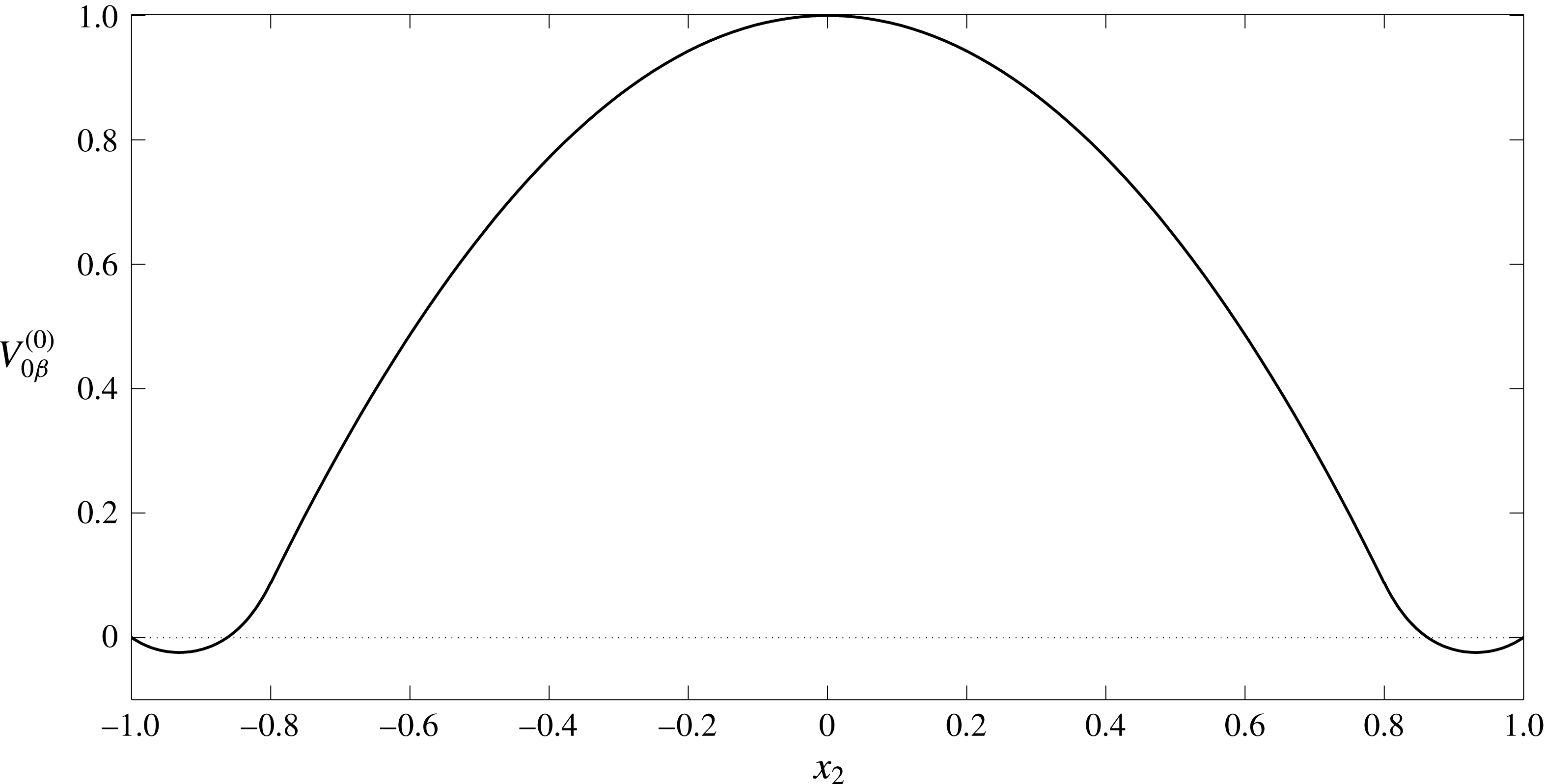
The velocity and displacement profiles in a straight-walled vessel are given by (A 9)–(A 11) and shown in figures 9, 10. In the EGL we observe negative velocity values near to the vessel wall. This reverse flow is due to the presence of the streaming potential. To better understand the nature of the reverse flow let us analyse the profile for the electric current,
 $i_{\unicode[STIX]{x1D6FD}}^{(0)}$
(see figure 11). It can be seen that there is a region with a negative value of current (near the wall), where the current direction is opposite to the flow direction in the core lumen. This results in an additional hydrodynamic resistivity (electroviscous effect). In the EGL the flow is retarded by the porous media resistance as well as by the reverse current, which at some point results in the appearance of the reverse flow.
Profile of elastic displacement
 $U^{(0)}$
across the EGL in a straight-walled vessel (A 11). The EGL has thickness
 $\unicode[STIX]{x1D700}=0.2$
.
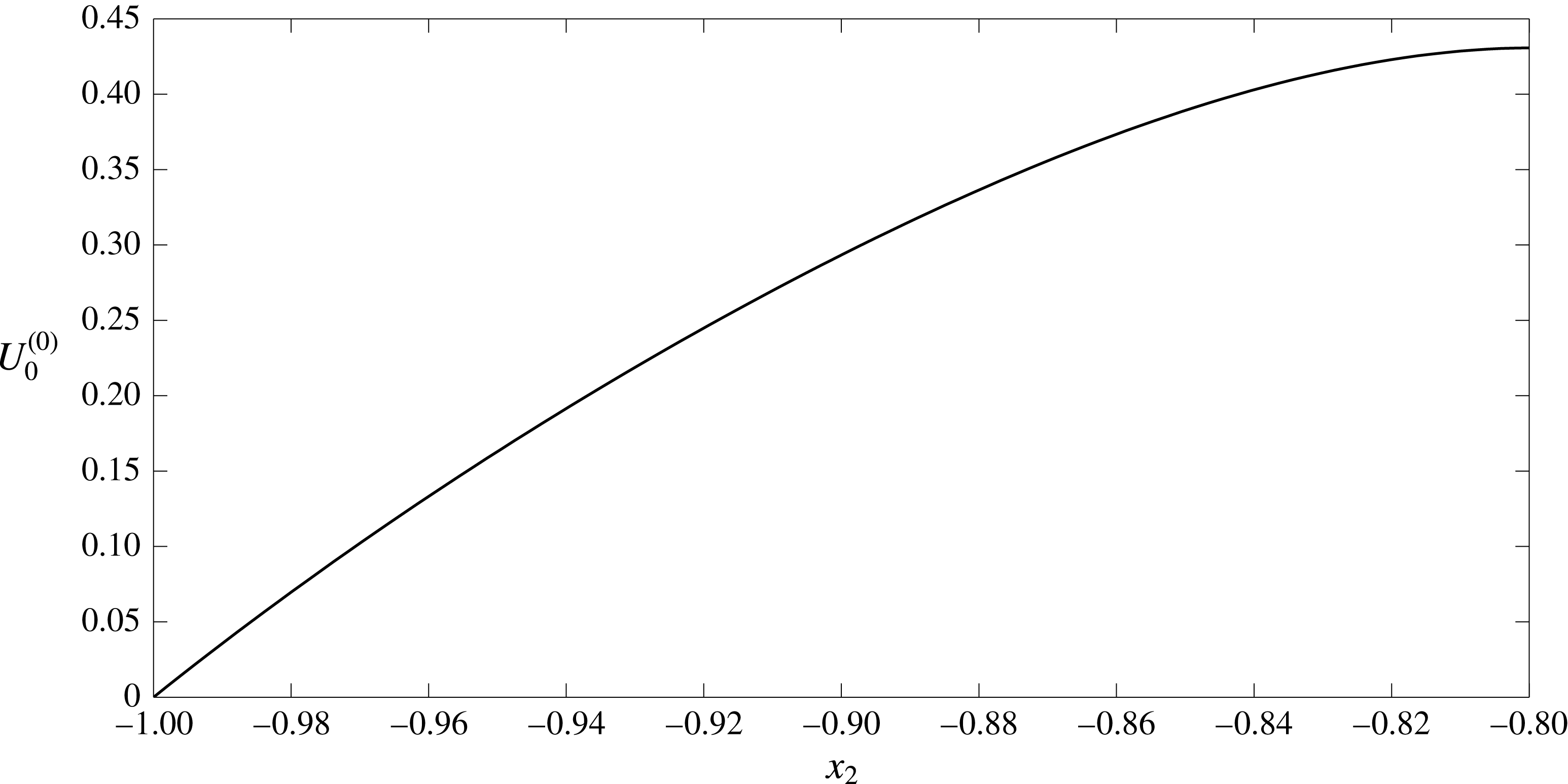
Electric current profile across the straight-walled vessel. The EGL has thickness
 $\unicode[STIX]{x1D700}=0.2$
and hence the electric current is given by
 $i_{l}^{(0)}$
for
 $-0.8<x_{2}<0.8$
and
 $i_{f}^{(0)}$
elsewhere.
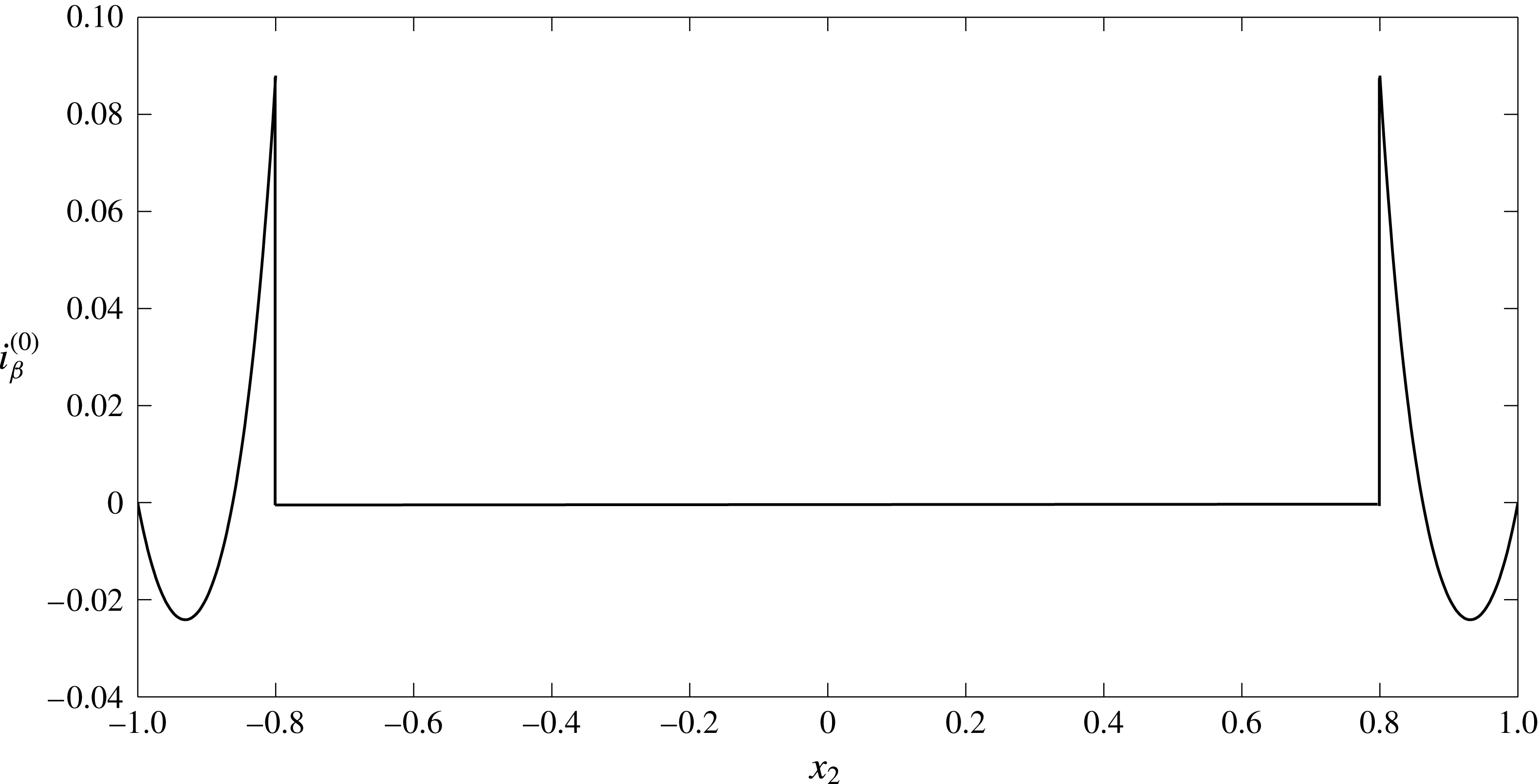
Appendix B. Debye layer analysis
First, let us consider the fluid phase in regions I and II. Describing the interface location by the smooth function
 $x_{2}=f(x_{1})$
, we can approximate its shape local to a point on the interface
 $(a,b)$
by the curve,
 $$\begin{eqnarray}X_{2}=X_{1}f^{\prime }(a)+f^{\prime \prime }(a)(X_{1}^{2}/2)+\cdots \,,\end{eqnarray}$$
where
 $X_{2}=x_{2}-b$
and
 $X_{1}=x_{1}-a$
. We consider the case where
 $f^{\prime }\ll 1$
,
 $f^{\prime \prime }\ll 1$
etc.’, which means that we can approximate the interface as lying at
 $X_{2}=0$
, and define
 $X_{2}>0$
as in the lumen, and
 $X_{2}<0$
as in the EGL (see figure 12). It is worth noting that if we were to consider surfaces with finite curvature, we would need
 $X_{1}\ll \unicode[STIX]{x1D6FF}^{1/2}$
, i.e. an asymptotically small inner region, which would need to asymptotically match to inner regions local to adjacent points on the interface. Under these circumstances, the type of finite-curvature analysis given by Yariv et al. (Reference Yariv, Schnitzer and Frankel2011) and Cox (Reference Cox1997) is necessary. Under our small-curvature approximation, the higher-order terms in (B 1) can lead to additional curvature terms in the governing equations, however, for sufficiently small curvatures these can be made subdominant to the retained terms (which are in terms of Debye layer thickness). Hence we describe the Debye layer in this regime using the scaled variables
 $$\begin{eqnarray}\displaystyle X_{1}=\unicode[STIX]{x1D709},\quad X_{2}=\unicode[STIX]{x1D6FF}\unicode[STIX]{x1D702},\quad v_{\unicode[STIX]{x1D6FD}1}=\tilde{v}_{\unicode[STIX]{x1D6FD}1},\quad v_{\unicode[STIX]{x1D6FD}2}=\unicode[STIX]{x1D6FF}\tilde{v}_{\unicode[STIX]{x1D6FD}2},\quad \tilde{c}_{\unicode[STIX]{x1D6FD}\pm }=c_{\unicode[STIX]{x1D6FD}\pm }(\unicode[STIX]{x1D709},\unicode[STIX]{x1D702}),\quad \tilde{\unicode[STIX]{x1D711}}_{\unicode[STIX]{x1D6FD}}=\unicode[STIX]{x1D711}_{\unicode[STIX]{x1D6FD}}(\unicode[STIX]{x1D709},\unicode[STIX]{x1D702}). & & \displaystyle \nonumber\\ \displaystyle & & \displaystyle\end{eqnarray}$$
(It can also be shown that there is no consistent solution with an
 $O(1)$
vertical flow through the layer; see appendix C.)
Schematic definition of a local Cartesian system (
 $X_{1},X_{2}$
) at the interface boundary and the rescaled coordinate system (
 $\unicode[STIX]{x1D709},\unicode[STIX]{x1D702}$
) describing the Debye layer.

Under the Debye layer rescalings (B 2), (3.1)–(3.5) (excluding (3.2)) take the form:
 $$\begin{eqnarray}\unicode[STIX]{x1D6FF}^{2}\frac{\unicode[STIX]{x2202}^{2}(\tilde{v}_{\unicode[STIX]{x1D6FD}})_{1}}{\unicode[STIX]{x2202}\unicode[STIX]{x1D709}^{2}}+\frac{\unicode[STIX]{x2202}^{2}(\tilde{v}_{\unicode[STIX]{x1D6FD}})_{1}}{\unicode[STIX]{x2202}\unicode[STIX]{x1D702}^{2}}=\unicode[STIX]{x1D6FF}^{2}\frac{\unicode[STIX]{x2202}\tilde{p}_{\unicode[STIX]{x1D6FD}}}{\unicode[STIX]{x2202}\unicode[STIX]{x1D709}}+\unicode[STIX]{x1D6FC}_{\unicode[STIX]{x1D6FD}}\frac{\unicode[STIX]{x2202}}{\unicode[STIX]{x2202}\unicode[STIX]{x1D709}}(\tilde{c}_{\unicode[STIX]{x1D6FD}+}+\tilde{c}_{\unicode[STIX]{x1D6FD}-})+\unicode[STIX]{x1D6FC}_{\unicode[STIX]{x1D6FD}}(\tilde{c}_{\unicode[STIX]{x1D6FD}+}-\tilde{c}_{\unicode[STIX]{x1D6FD}-})\frac{\unicode[STIX]{x2202}\tilde{\unicode[STIX]{x1D711}}_{\unicode[STIX]{x1D6FD}}}{\unicode[STIX]{x2202}\unicode[STIX]{x1D709}}+\unicode[STIX]{x1D6FF}^{2}\unicode[STIX]{x1D712}h_{\unicode[STIX]{x1D6FD}}(\tilde{v}_{\unicode[STIX]{x1D6FD}})_{1},\end{eqnarray}$$
 $$\begin{eqnarray}\unicode[STIX]{x1D6FF}^{4}\frac{\unicode[STIX]{x2202}^{2}(\tilde{v}_{\unicode[STIX]{x1D6FD}})_{2}}{\unicode[STIX]{x2202}\unicode[STIX]{x1D709}^{2}}+\unicode[STIX]{x1D6FF}^{2}\frac{\unicode[STIX]{x2202}^{2}(\tilde{v}_{\unicode[STIX]{x1D6FD}})_{2}}{\unicode[STIX]{x2202}\unicode[STIX]{x1D702}^{2}}=\unicode[STIX]{x1D6FF}^{2}\frac{\unicode[STIX]{x2202}\tilde{p}_{\unicode[STIX]{x1D6FD}}}{\unicode[STIX]{x2202}\unicode[STIX]{x1D702}}+\unicode[STIX]{x1D6FC}_{\unicode[STIX]{x1D6FD}}\frac{\unicode[STIX]{x2202}}{\unicode[STIX]{x2202}\unicode[STIX]{x1D702}}(\tilde{c}_{\unicode[STIX]{x1D6FD}+}+\tilde{c}_{\unicode[STIX]{x1D6FD}-})+\unicode[STIX]{x1D6FC}_{\unicode[STIX]{x1D6FD}}(\tilde{c}_{\unicode[STIX]{x1D6FD}+}-\tilde{c}_{\unicode[STIX]{x1D6FD}-})\frac{\unicode[STIX]{x2202}\tilde{\unicode[STIX]{x1D711}}_{\unicode[STIX]{x1D6FD}}}{\unicode[STIX]{x2202}\unicode[STIX]{x1D702}}+\unicode[STIX]{x1D6FF}^{4}\unicode[STIX]{x1D712}h_{\unicode[STIX]{x1D6FD}}(\tilde{v}_{\unicode[STIX]{x1D6FD}})_{2},\end{eqnarray}$$
 $$\begin{eqnarray}\frac{\unicode[STIX]{x2202}(\tilde{v}_{\unicode[STIX]{x1D6FD}})_{1}}{\unicode[STIX]{x2202}\unicode[STIX]{x1D709}}+\frac{\unicode[STIX]{x2202}(\tilde{v}_{\unicode[STIX]{x1D6FD}})_{2}}{\unicode[STIX]{x2202}\unicode[STIX]{x1D702}}=0,\end{eqnarray}$$
 $$\begin{eqnarray}\displaystyle & & \displaystyle \unicode[STIX]{x1D6FE}_{\pm }\unicode[STIX]{x1D6FF}^{2}\left((\tilde{v}_{\unicode[STIX]{x1D6FD}})_{1}\frac{\unicode[STIX]{x2202}\tilde{c}_{\unicode[STIX]{x1D6FD}\pm }}{\unicode[STIX]{x2202}\unicode[STIX]{x1D709}}+(\tilde{v}_{\unicode[STIX]{x1D6FD}})_{2}\frac{\unicode[STIX]{x2202}\tilde{c}_{\unicode[STIX]{x1D6FD}\pm }}{\unicode[STIX]{x2202}\unicode[STIX]{x1D702}}\right)-\unicode[STIX]{x1D6FF}^{2}\frac{\unicode[STIX]{x2202}^{2}\tilde{c}_{\unicode[STIX]{x1D6FD}\pm }}{\unicode[STIX]{x2202}\unicode[STIX]{x1D709}^{2}}-\frac{\unicode[STIX]{x2202}^{2}\tilde{c}_{\unicode[STIX]{x1D6FD}\pm }}{\unicode[STIX]{x2202}\unicode[STIX]{x1D702}^{2}}\nonumber\\ \displaystyle & & \displaystyle \quad \mp \left(\unicode[STIX]{x1D6FF}^{2}\frac{\unicode[STIX]{x2202}\tilde{c}_{\unicode[STIX]{x1D6FD}\pm }}{\unicode[STIX]{x2202}\unicode[STIX]{x1D709}}\frac{\unicode[STIX]{x2202}\tilde{\unicode[STIX]{x1D711}}_{\unicode[STIX]{x1D6FD}}}{\unicode[STIX]{x2202}\unicode[STIX]{x1D709}}+\frac{\unicode[STIX]{x2202}\tilde{c}_{\unicode[STIX]{x1D6FD}\pm }}{\unicode[STIX]{x2202}\unicode[STIX]{x1D702}}\frac{\unicode[STIX]{x2202}\tilde{\unicode[STIX]{x1D711}}_{\unicode[STIX]{x1D6FD}}}{\unicode[STIX]{x2202}\unicode[STIX]{x1D702}}+\unicode[STIX]{x1D6FF}^{2}\tilde{c}_{\unicode[STIX]{x1D6FD}\pm }\frac{\unicode[STIX]{x2202}^{2}\tilde{\unicode[STIX]{x1D711}}_{\unicode[STIX]{x1D6FD}}}{\unicode[STIX]{x2202}\unicode[STIX]{x1D709}^{2}}+\tilde{c}_{\unicode[STIX]{x1D6FD}\pm }\frac{\unicode[STIX]{x2202}^{2}\tilde{\unicode[STIX]{x1D711}}_{\unicode[STIX]{x1D6FD}}}{\unicode[STIX]{x2202}\unicode[STIX]{x1D702}^{2}}\right)=0,\end{eqnarray}$$
 $$\begin{eqnarray}-\unicode[STIX]{x1D6FF}^{2}\frac{\unicode[STIX]{x2202}^{2}\tilde{\unicode[STIX]{x1D711}}_{\unicode[STIX]{x1D6FD}}}{\unicode[STIX]{x2202}\unicode[STIX]{x1D709}^{2}}-\frac{\unicode[STIX]{x2202}^{2}\tilde{\unicode[STIX]{x1D711}}_{\unicode[STIX]{x1D6FD}}}{\unicode[STIX]{x2202}\unicode[STIX]{x1D702}^{2}}=\tilde{c}_{\unicode[STIX]{x1D6FD}+}-\tilde{c}_{\unicode[STIX]{x1D6FD}-}-h_{\unicode[STIX]{x1D6FD}}c_{s}.\end{eqnarray}$$
The following continuity boundary conditions need to be met on the interface,
 $\unicode[STIX]{x1D702}=0$
 $$\begin{eqnarray}\tilde{\boldsymbol{v}}_{l}=\unicode[STIX]{x1D719}_{f}\tilde{\boldsymbol{v}}_{f},\quad \tilde{\unicode[STIX]{x1D711}}_{l}=\tilde{\unicode[STIX]{x1D711}}_{f},\quad \frac{\unicode[STIX]{x2202}\tilde{\unicode[STIX]{x1D711}}_{l}}{\unicode[STIX]{x2202}n}=\frac{\unicode[STIX]{x2202}\tilde{\unicode[STIX]{x1D711}}_{f}}{\unicode[STIX]{x2202}n},\quad \tilde{c}_{l\pm }=\tilde{c}_{f\pm },\quad \frac{\unicode[STIX]{x2202}\tilde{c}_{l\pm }}{\unicode[STIX]{x2202}n}=\frac{\unicode[STIX]{x2202}\tilde{c}_{f\pm }}{\unicode[STIX]{x2202}n}.\end{eqnarray}$$
Now we introduce an inner expansion
 $\tilde{f}=\tilde{f}^{(0)}+\unicode[STIX]{x1D6FF}^{2}\tilde{f}^{(1)}+\cdots \,$
. Quantities in the Debye layer must also match to their counterparts in the bulk lumen/EGL, i.e.
 $$\begin{eqnarray}\lim _{\unicode[STIX]{x1D702}\rightarrow \infty }(\tilde{f}^{(0)}(\unicode[STIX]{x1D709},\unicode[STIX]{x1D702})+\unicode[STIX]{x1D6FF}^{2}\tilde{f}^{(1)}(\unicode[STIX]{x1D709},\unicode[STIX]{x1D702})+\cdots \,)=\lim _{X_{2}\rightarrow 0}(f^{(0)}(X_{1},X_{2})+\unicode[STIX]{x1D6FF}^{2}f^{(1)}(X_{1},X_{2})+\cdots \,),\end{eqnarray}$$
where
 $X_{2}=0$
is the vertical position of the interface in the outer problem.
Leading-order solution
The governing equations at
 $O(1)$
are the following
 $$\begin{eqnarray}\frac{\unicode[STIX]{x2202}^{2}(\tilde{v}_{\unicode[STIX]{x1D6FD}}^{(0)})_{1}}{\unicode[STIX]{x2202}\unicode[STIX]{x1D702}^{2}}=\unicode[STIX]{x1D6FC}_{\unicode[STIX]{x1D6FD}}\frac{\unicode[STIX]{x2202}}{\unicode[STIX]{x2202}\unicode[STIX]{x1D709}}(\tilde{c}_{\unicode[STIX]{x1D6FD}+}^{(0)}+\tilde{c}_{\unicode[STIX]{x1D6FD}-}^{(0)})+\unicode[STIX]{x1D6FC}_{\unicode[STIX]{x1D6FD}}(\tilde{c}_{\unicode[STIX]{x1D6FD}+}^{(0)}-\tilde{c}_{\unicode[STIX]{x1D6FD}-}^{(0)})\frac{\unicode[STIX]{x2202}\tilde{\unicode[STIX]{x1D711}}_{\unicode[STIX]{x1D6FD}}^{(0)}}{\unicode[STIX]{x2202}\unicode[STIX]{x1D709}},\end{eqnarray}$$
 $$\begin{eqnarray}0=\frac{\unicode[STIX]{x2202}}{\unicode[STIX]{x2202}\unicode[STIX]{x1D702}}(\tilde{c}_{\unicode[STIX]{x1D6FD}+}^{(0)}+\tilde{c}_{\unicode[STIX]{x1D6FD}-}^{(0)})+(\tilde{c}_{\unicode[STIX]{x1D6FD}+}^{(0)}-\tilde{c}_{\unicode[STIX]{x1D6FD}-}^{(0)})\frac{\unicode[STIX]{x2202}\tilde{\unicode[STIX]{x1D711}}_{\unicode[STIX]{x1D6FD}}^{(0)}}{\unicode[STIX]{x2202}\unicode[STIX]{x1D702}},\end{eqnarray}$$
 $$\begin{eqnarray}\frac{\unicode[STIX]{x2202}(\tilde{v}_{\unicode[STIX]{x1D6FD}}^{(0)})_{1}}{\unicode[STIX]{x2202}\unicode[STIX]{x1D709}}+\frac{\unicode[STIX]{x2202}(\tilde{v}_{\unicode[STIX]{x1D6FD}}^{(0)})_{2}}{\unicode[STIX]{x2202}\unicode[STIX]{x1D702}}=0,\end{eqnarray}$$
 $$\begin{eqnarray}-\frac{\unicode[STIX]{x2202}^{2}\tilde{c}_{\unicode[STIX]{x1D6FD}\pm }^{(0)}}{\unicode[STIX]{x2202}\unicode[STIX]{x1D702}^{2}}\mp \frac{\unicode[STIX]{x2202}}{\unicode[STIX]{x2202}\unicode[STIX]{x1D702}}\left(\tilde{c}_{\unicode[STIX]{x1D6FD}\pm }^{(0)}\frac{\unicode[STIX]{x2202}\tilde{\unicode[STIX]{x1D711}}_{\unicode[STIX]{x1D6FD}}^{(0)}}{\unicode[STIX]{x2202}\unicode[STIX]{x1D702}}\right)=0,\end{eqnarray}$$
 $$\begin{eqnarray}-\frac{\unicode[STIX]{x2202}^{2}\tilde{\unicode[STIX]{x1D711}}_{\unicode[STIX]{x1D6FD}}^{(0)}}{\unicode[STIX]{x2202}\unicode[STIX]{x1D702}^{2}}=\tilde{c}_{\unicode[STIX]{x1D6FD}+}^{(0)}-\tilde{c}_{\unicode[STIX]{x1D6FD}-}^{(0)}-h_{\unicode[STIX]{x1D6FD}}c_{s}.\end{eqnarray}$$
Solutions to equations (B 13)–(B 14) are sought in the form:
 $\tilde{c}_{\unicode[STIX]{x1D6FD}\pm }^{(0)}=\tilde{c}_{\unicode[STIX]{x1D6FD}\pm }^{(0)}(\unicode[STIX]{x1D702})$
,
 $\tilde{\unicode[STIX]{x1D711}}_{\unicode[STIX]{x1D6FD}}^{(0)}=\tilde{\unicode[STIX]{x1D711}}_{\unicode[STIX]{x1D6FD}}^{(0)}(\unicode[STIX]{x1D702})$
(since in the outer region
 $\unicode[STIX]{x1D711}_{\unicode[STIX]{x1D6FD}}^{(0)}$
and
 $c_{\unicode[STIX]{x1D6FD}\pm }^{(0)}$
are constants (3.10)). In addition,
 $\tilde{c}_{\unicode[STIX]{x1D6FD}\pm }^{(0)}$
and
 $\tilde{\unicode[STIX]{x1D711}}_{\unicode[STIX]{x1D6FD}}^{(0)}$
are bounded in the far field (
 ${\tilde{c}_{\unicode[STIX]{x1D6FD}\pm }}^{(0)^{\prime }}=0$
and
 ${\tilde{\unicode[STIX]{x1D711}}_{\unicode[STIX]{x1D6FD}}}^{(0)^{\prime }}=0$
as
 $\unicode[STIX]{x1D702}\rightarrow \infty$
). We obtain
 $$\begin{eqnarray}-{\tilde{c}_{\unicode[STIX]{x1D6FD}\pm }}^{\prime \prime (0)}\mp (\tilde{c}_{\unicode[STIX]{x1D6FD}\pm }^{(0)}{\tilde{\unicode[STIX]{x1D711}}_{\unicode[STIX]{x1D6FD}}}^{\prime (0)})^{\prime }=0,\end{eqnarray}$$
 $$\begin{eqnarray}-{\tilde{\unicode[STIX]{x1D711}}_{\unicode[STIX]{x1D6FD}}}^{\prime \prime (0)}=\tilde{c}_{\unicode[STIX]{x1D6FD}+}^{(0)}-\tilde{c}_{\unicode[STIX]{x1D6FD}-}^{(0)}-h_{\unicode[STIX]{x1D6FD}}c_{s},\end{eqnarray}$$
where prime denotes derivatives with respect to
 $\unicode[STIX]{x1D702}$
. For the ion distributions we obtain
 $$\begin{eqnarray}\displaystyle -{\tilde{c}_{\unicode[STIX]{x1D6FD}\pm }}^{\prime (0)}\mp \tilde{c}_{\unicode[STIX]{x1D6FD}\pm }^{(0)}\tilde{\unicode[STIX]{x1D711}}^{\prime (0)}=A_{\pm }. & & \displaystyle\end{eqnarray}$$
As
 ${\tilde{c}_{\unicode[STIX]{x1D6FD}\pm }}^{\prime (0)}(\unicode[STIX]{x1D702}\rightarrow \infty )=0$
,
 ${\tilde{\unicode[STIX]{x1D711}}_{\unicode[STIX]{x1D6FD}}}^{\prime (0)}(\unicode[STIX]{x1D702}\rightarrow \infty )=0$
and
 $\tilde{c}_{\unicode[STIX]{x1D6FD}\pm }^{(0)}(\unicode[STIX]{x1D702}\rightarrow \infty )$
is bounded (as they must match to constant ion concentrations and potentials in the bulk lumen/EGL), then
 $A_{\pm }=0$
. Therefore,
 $-{\tilde{c}_{\unicode[STIX]{x1D6FD}\pm }}^{\prime (0)}\mp {\tilde{c}_{\unicode[STIX]{x1D6FD}\pm }}^{(0)}{\tilde{\unicode[STIX]{x1D711}}_{\unicode[STIX]{x1D6FD}}}^{\prime (0)}=0$
and
 $\tilde{c}_{\unicode[STIX]{x1D6FD}\pm }^{(0)}=B_{\unicode[STIX]{x1D6FD}\pm }e^{\mp \tilde{\unicode[STIX]{x1D711}}_{\unicode[STIX]{x1D6FD}}^{(0)}}$
. Since from (3.10)
 $\tilde{c}_{l+}^{(0)}(\unicode[STIX]{x1D702}\rightarrow +\infty )=\tilde{c}_{l-}^{(0)}(\unicode[STIX]{x1D702}\rightarrow +\infty )=1$
and
 $\tilde{\unicode[STIX]{x1D711}}_{l}^{(0)}\rightarrow 0$
then
 $B_{l+}=B_{l-}=1$
. From the continuity boundary conditions at the interface (B 8) we can also deduce that
 $B_{f\pm }=B_{l\pm }=1$
. We therefore arrive at the equations for the electric potential in the EGL
 $$\begin{eqnarray}\displaystyle & & \displaystyle {\tilde{\unicode[STIX]{x1D711}}_{\unicode[STIX]{x1D6FD}}}^{\prime \prime (0)}=2\sinh \tilde{\unicode[STIX]{x1D711}}_{\unicode[STIX]{x1D6FD}}^{(0)}+h_{\unicode[STIX]{x1D6FD}}c_{s}.\end{eqnarray}$$
Equation (B 18) allows us to find a potential jump value across the Debye layer without the need to find the actual solution. Since
 $\tilde{\unicode[STIX]{x1D711}}_{f}^{(0)}\rightarrow K$
(constant) as
 $\unicode[STIX]{x1D702}\rightarrow -\infty$
through matching to the bulk lumen/EGL, we conclude that
 ${\tilde{\unicode[STIX]{x1D711}}_{f}}^{\prime \prime (0)}\rightarrow 0$
. From (B 18) we obtain the limiting form
 $$\begin{eqnarray}\displaystyle & & \displaystyle 0=2\sinh \tilde{\unicode[STIX]{x1D711}}_{\unicode[STIX]{x1D6FD}}^{(0)}(-\infty )+h_{\unicode[STIX]{x1D6FD}}c_{s}.\end{eqnarray}$$
As a result we have
 $$\begin{eqnarray}\tilde{\unicode[STIX]{x1D711}}_{l}^{(0)}(+\infty )=0,\quad \tilde{\unicode[STIX]{x1D711}}_{f}^{(0)}(-\infty )=\operatorname{arcsinh}\left(-\frac{c_{s}}{2}\right),\end{eqnarray}$$
and, hence, the jump
 $[\unicode[STIX]{x1D711}_{\unicode[STIX]{x1D6FD}}^{(0)}]=\operatorname{arcsinh}(-c_{s}/2)$
. Accordingly,
 $$\begin{eqnarray}\tilde{c}_{l+}^{(0)}(+\infty )=\tilde{c}_{l-}^{(0)}(+\infty )=1,\end{eqnarray}$$
 $$\begin{eqnarray}\tilde{c}_{f+}^{(0)}(-\infty )=\exp \!\left(-\text{arcsinh}\left(-\frac{c_{s}}{2}\right)\right),\quad \tilde{c}_{f-}^{(0)}(-\infty )=\exp \!\left(\operatorname{arcsinh}\left(-\frac{c_{s}}{2}\right)\right).\end{eqnarray}$$
Numerical solutions to (B 18) are shown in figure 13 and show that the predicted value of the jumps are correct. Ion concentration distributions can be seen on figure 14. Numerical solutions were obtained using the bvp4c MATLAB routine which solves boundary value problems for ordinary differential equations. The infinitely long integration interval
 $(-\infty ,+\infty )$
is replaced by the finite length
 $[-a,a]$
where the value of
 $a$
is increased until convergence is reached (which occurs here at approximately
 $a=10$
).
Distribution of the electric potential
 $\tilde{\unicode[STIX]{x1D711}}_{\unicode[STIX]{x1D6FD}}^{(0)}$
(——) across the Debye layer, showing a jump in value of
 $[\unicode[STIX]{x1D711}_{\unicode[STIX]{x1D6FD}}^{(0)}]=\operatorname{arcsinh}(-c_{s}/2)$
(- - - -) with
 $c_{s}=1$
.

Distribution of the positive
 $\tilde{c}_{\unicode[STIX]{x1D6FD}+}^{(0)}$
(- - - -) and negative
 $\tilde{c}_{\unicode[STIX]{x1D6FD}-}^{(0)}$
(——) ions concentrations across the Debye layer alongside the limited values predicted by (B 22a,b
) ((— ⋅ —) and (
 $\cdots \cdots$
)) when
 $c_{s}=1$
.

We now consider the leading-order velocities. Since
 $\tilde{\unicode[STIX]{x1D711}}_{\unicode[STIX]{x1D6FD}}^{(0)}$
and
 $\tilde{c}_{\unicode[STIX]{x1D6FD}\pm }^{(0)}$
depend only on
 $\unicode[STIX]{x1D702}$
, then (B 10)–(B 12) reduce to
 $$\begin{eqnarray}\displaystyle & \displaystyle \frac{\unicode[STIX]{x2202}^{2}(\tilde{v}_{\unicode[STIX]{x1D6FD}}^{(0)})_{1}}{\unicode[STIX]{x2202}\unicode[STIX]{x1D702}^{2}}=0, & \displaystyle\end{eqnarray}$$
 $$\begin{eqnarray}\displaystyle & \displaystyle \frac{\unicode[STIX]{x2202}(\tilde{v}_{\unicode[STIX]{x1D6FD}}^{(0)})_{1}}{\unicode[STIX]{x2202}\unicode[STIX]{x1D709}}=-\frac{\unicode[STIX]{x2202}(\tilde{v}_{\unicode[STIX]{x1D6FD}}^{(0)})_{2}}{\unicode[STIX]{x2202}\unicode[STIX]{x1D702}}, & \displaystyle\end{eqnarray}$$
where
 $(\boldsymbol{v}_{\unicode[STIX]{x1D6FD}}^{(0)})_{i}$
denotes the
 $i$
th component of
 $\boldsymbol{v}_{\unicode[STIX]{x1D6FD}}^{(0)}$
. From (B 23) we obtain
 $$\begin{eqnarray}(\tilde{v}_{\unicode[STIX]{x1D6FD}}^{(0)})_{1}={\mathcal{V}}_{\unicode[STIX]{x1D6FD}}(\unicode[STIX]{x1D709})\unicode[STIX]{x1D702}+V_{\unicode[STIX]{x1D6FD}}(\unicode[STIX]{x1D709}).\end{eqnarray}$$
From the matching condition (B 9) we see
 $$\begin{eqnarray}\displaystyle \lim _{\unicode[STIX]{x1D702}\rightarrow \infty }({\mathcal{V}}_{\unicode[STIX]{x1D6FD}}(\unicode[STIX]{x1D709})\unicode[STIX]{x1D702}+V_{\unicode[STIX]{x1D6FD}}(\unicode[STIX]{x1D709})+\cdots \,\!)=\lim _{X_{2}\rightarrow 0}((v_{\unicode[STIX]{x1D6FD}}^{(0)})_{1}(X_{1},X_{2})+\cdots \!\,), & & \displaystyle\end{eqnarray}$$
and so
 ${\mathcal{V}}_{\unicode[STIX]{x1D6FD}}=0$
(to avoid unbounded growth),
 $V_{\unicode[STIX]{x1D6FD}}(X_{1})=(v_{\unicode[STIX]{x1D6FD}}^{(0)})_{1}(X_{1},0)$
, i.e. the bulk flow slip velocity at the interface.
The vertical component of the velocity found from (B 24) has the form
 $(\tilde{v}_{\unicode[STIX]{x1D6FD}}^{(0)})_{2}=-V_{\unicode[STIX]{x1D6FD}}^{\prime }(\unicode[STIX]{x1D709})\unicode[STIX]{x1D702}+W_{\unicode[STIX]{x1D6FD}}(\unicode[STIX]{x1D709})$
. The matching condition demands that
 $$\begin{eqnarray}\displaystyle \lim _{\unicode[STIX]{x1D702}\rightarrow \infty }(\unicode[STIX]{x1D6FF}(\tilde{v}_{\unicode[STIX]{x1D6FD}}^{(0)})_{2}(\unicode[STIX]{x1D709},\unicode[STIX]{x1D702})+\cdots \,)=\lim _{X_{2}\rightarrow 0}((v_{\unicode[STIX]{x1D6FD}}^{(0)})_{2}(X_{1},X_{2})+\cdots \,). & & \displaystyle\end{eqnarray}$$
Taking a power series expansion of
 $(v_{\unicode[STIX]{x1D6FD}}^{(0)})_{2}(X_{1},X_{2})$
about
 $X_{2}=0$
, and using continuity in the outer flow we can rewrite (B 27) as
 $$\begin{eqnarray}\displaystyle -\unicode[STIX]{x1D702}\unicode[STIX]{x1D6FF}V_{\unicode[STIX]{x1D6FD}}^{\prime }(\unicode[STIX]{x1D709})+\unicode[STIX]{x1D6FF}W_{\unicode[STIX]{x1D6FD}}(\unicode[STIX]{x1D709})+\cdots =(v_{\unicode[STIX]{x1D6FD}}^{(0)})_{2}(\unicode[STIX]{x1D709},0)-\unicode[STIX]{x1D702}\unicode[STIX]{x1D6FF}\frac{\unicode[STIX]{x2202}(v_{\unicode[STIX]{x1D6FD}}^{(0)})_{1}(\unicode[STIX]{x1D709},0)}{\unicode[STIX]{x2202}\unicode[STIX]{x1D709}}\ldots . & & \displaystyle\end{eqnarray}$$
We conclude that
 $W_{\unicode[STIX]{x1D6FD}}=0$
and
 $(v_{\unicode[STIX]{x1D6FD}}^{(0)})_{2}(\unicode[STIX]{x1D709},0)=0$
. Hence, in summary, we have
 $$\begin{eqnarray}\displaystyle & & \displaystyle (\tilde{v}_{\unicode[STIX]{x1D6FD}}^{(0)})_{1}=V_{\unicode[STIX]{x1D6FD}}(\unicode[STIX]{x1D709}),\quad (\tilde{v}_{\unicode[STIX]{x1D6FD}}^{(0)})_{2}=-V_{\unicode[STIX]{x1D6FD}}^{\prime }(\unicode[STIX]{x1D709})\unicode[STIX]{x1D702}.\end{eqnarray}$$
In summary, the leading-order Debye layer analysis tells us the constant values for the potential and ion concentrations at leading order in the bulk lumen and EGL, as well as how the leading-order flow transits the Debye layer. In order to determine boundary conditions for the next-order corrections which drive the leading-order flow in the bulk lumen/EGL, it is necessary to go to next order in the Debye layer.
First-order corrections
Since the leading-order flows in the bulk EGL (lumen) are driven by
 $c_{\unicode[STIX]{x1D6FD}}^{(1)}$
and
 $\unicode[STIX]{x1D719}_{\unicode[STIX]{x1D6FD}}^{(1)}$
, it is necessary to determine the quantities at next order in the Debye layer. At
 $O(\unicode[STIX]{x1D6FF})$
in this inner region, the equations take the form:
 $$\begin{eqnarray}\displaystyle \frac{\unicode[STIX]{x2202}^{2}(\tilde{v}_{\unicode[STIX]{x1D6FD}}^{(0)})_{1}}{\unicode[STIX]{x2202}\unicode[STIX]{x1D709}^{2}}+\frac{\unicode[STIX]{x2202}^{2}(\tilde{v}_{\unicode[STIX]{x1D6FD}}^{(1)})_{1}}{\unicode[STIX]{x2202}\unicode[STIX]{x1D702}^{2}} & = & \displaystyle \frac{\unicode[STIX]{x2202}\tilde{p}_{\unicode[STIX]{x1D6FD}}^{(0)}}{\unicode[STIX]{x2202}\unicode[STIX]{x1D709}}+\unicode[STIX]{x1D6FC}_{\unicode[STIX]{x1D6FD}}\frac{\unicode[STIX]{x2202}}{\unicode[STIX]{x2202}\unicode[STIX]{x1D709}}(\tilde{c}_{\unicode[STIX]{x1D6FD}+}^{(1)}+\tilde{c}_{\unicode[STIX]{x1D6FD}-}^{(1)})+\unicode[STIX]{x1D6FC}_{\unicode[STIX]{x1D6FD}}(\tilde{c}_{\unicode[STIX]{x1D6FD}+}^{(0)}-\tilde{c}_{\unicode[STIX]{x1D6FD}-}^{(0)})\frac{\unicode[STIX]{x2202}\tilde{\unicode[STIX]{x1D711}}_{\unicode[STIX]{x1D6FD}}^{(1)}}{\unicode[STIX]{x2202}\unicode[STIX]{x1D709}}\nonumber\\ \displaystyle & & \displaystyle +\,\unicode[STIX]{x1D6FC}_{\unicode[STIX]{x1D6FD}}(\tilde{c}_{\unicode[STIX]{x1D6FD}+}^{(1)}-\tilde{c}_{\unicode[STIX]{x1D6FD}-}^{(1)})\frac{\unicode[STIX]{x2202}\tilde{\unicode[STIX]{x1D711}}_{\unicode[STIX]{x1D6FD}}^{(0)}}{\unicode[STIX]{x2202}\unicode[STIX]{x1D709}}+\unicode[STIX]{x1D712}h_{\unicode[STIX]{x1D6FD}}\tilde{v}_{\unicode[STIX]{x1D6FD}1}^{(0)},\end{eqnarray}$$
 $$\begin{eqnarray}\displaystyle 0 & = & \displaystyle \frac{\unicode[STIX]{x2202}\tilde{p}_{\unicode[STIX]{x1D6FD}}^{(0)}}{\unicode[STIX]{x2202}\unicode[STIX]{x1D702}}+\unicode[STIX]{x1D6FC}_{\unicode[STIX]{x1D6FD}}\frac{\unicode[STIX]{x2202}}{\unicode[STIX]{x2202}\unicode[STIX]{x1D702}}(\tilde{c}_{\unicode[STIX]{x1D6FD}+}^{(1)}+\tilde{c}_{\unicode[STIX]{x1D6FD}-}^{(1)})+\,\unicode[STIX]{x1D6FC}_{\unicode[STIX]{x1D6FD}}(\tilde{c}_{\unicode[STIX]{x1D6FD}+}^{(0)}-\tilde{c}_{\unicode[STIX]{x1D6FD}-}^{(0)})\frac{\unicode[STIX]{x2202}\tilde{\unicode[STIX]{x1D711}}_{\unicode[STIX]{x1D6FD}}^{(1)}}{\unicode[STIX]{x2202}\unicode[STIX]{x1D702}}+\unicode[STIX]{x1D6FC}_{\unicode[STIX]{x1D6FD}}(\tilde{c}_{\unicode[STIX]{x1D6FD}+}^{(1)}-\tilde{c}_{\unicode[STIX]{x1D6FD}-}^{(1)})\frac{\unicode[STIX]{x2202}\tilde{\unicode[STIX]{x1D711}}_{\unicode[STIX]{x1D6FD}}^{(0)}}{\unicode[STIX]{x2202}\unicode[STIX]{x1D702}},\qquad\end{eqnarray}$$
 $$\begin{eqnarray}\frac{\unicode[STIX]{x2202}(\tilde{v}_{\unicode[STIX]{x1D6FD}}^{(1)})_{1}}{\unicode[STIX]{x2202}\unicode[STIX]{x1D709}}+\frac{\unicode[STIX]{x2202}(\tilde{v}_{\unicode[STIX]{x1D6FD}}^{(1)})_{2}}{\unicode[STIX]{x2202}\unicode[STIX]{x1D702}}=0,\end{eqnarray}$$
 $$\begin{eqnarray}-\unicode[STIX]{x1D6FE}_{\pm }V_{\unicode[STIX]{x1D6FD}}^{\prime }(\unicode[STIX]{x1D709})\unicode[STIX]{x1D702}\frac{\unicode[STIX]{x2202}\tilde{c}_{\unicode[STIX]{x1D6FD}\pm }^{(0)}}{\unicode[STIX]{x2202}\unicode[STIX]{x1D702}}-\frac{\unicode[STIX]{x2202}^{2}\tilde{c}_{\unicode[STIX]{x1D6FD}\pm }^{(1)}}{\unicode[STIX]{x2202}\unicode[STIX]{x1D702}^{2}}\mp \frac{\unicode[STIX]{x2202}}{\unicode[STIX]{x2202}\unicode[STIX]{x1D702}}\left(\tilde{c}_{\unicode[STIX]{x1D6FD}\pm }^{(0)}\frac{\unicode[STIX]{x2202}\tilde{\unicode[STIX]{x1D711}}_{\unicode[STIX]{x1D6FD}}^{(1)}}{\unicode[STIX]{x2202}\unicode[STIX]{x1D702}}+\tilde{c}_{\unicode[STIX]{x1D6FD}\pm }^{(1)}\frac{\unicode[STIX]{x2202}\tilde{\unicode[STIX]{x1D711}}_{\unicode[STIX]{x1D6FD}}^{(0)}}{\unicode[STIX]{x2202}\unicode[STIX]{x1D702}}\right)=0,\end{eqnarray}$$
 $$\begin{eqnarray}-\frac{\unicode[STIX]{x2202}^{2}\tilde{\unicode[STIX]{x1D711}}_{\unicode[STIX]{x1D6FD}}^{(1)}}{\unicode[STIX]{x2202}\unicode[STIX]{x1D702}^{2}}=\tilde{c}_{\unicode[STIX]{x1D6FD}+}^{(1)}-\tilde{c}_{\unicode[STIX]{x1D6FD}-}^{(1)}.\end{eqnarray}$$
So for ion transport we obtain a linear equation (B 33) subject to the forcing terms
 $F_{\unicode[STIX]{x1D6FD}}=-\unicode[STIX]{x1D6FE}_{\pm }V_{\unicode[STIX]{x1D6FD}}^{\prime }(\unicode[STIX]{x1D709})\unicode[STIX]{x1D702}\unicode[STIX]{x2202}\tilde{c}_{\unicode[STIX]{x1D6FD}\pm }^{(0)}/\unicode[STIX]{x2202}\unicode[STIX]{x1D702}$
.
Mirroring the solution decomposition in the bulk EGL and lumen, we seek a solution as a sum of homogeneous and non-homogeneous parts,
 $$\begin{eqnarray}\tilde{c}_{\unicode[STIX]{x1D6FD}\pm }^{(1)}=\tilde{c}_{\unicode[STIX]{x1D6FD}h\pm }^{(1)}+\tilde{c}_{\unicode[STIX]{x1D6FD}p\pm }^{(1)},\quad \tilde{\unicode[STIX]{x1D711}}_{\unicode[STIX]{x1D6FD}}^{(1)}=\tilde{\unicode[STIX]{x1D711}}_{\unicode[STIX]{x1D6FD}h}^{(1)}+\tilde{\unicode[STIX]{x1D711}}_{\unicode[STIX]{x1D6FD}p}^{(1)},\end{eqnarray}$$
The homogeneous solution corresponds to the case where
 $F_{\unicode[STIX]{x1D6FD}}=0$
, and respects the inner boundary conditions (B 8) as well as matches to
 $c_{\pm }^{(1)}=0$
in the bulk lumen/EGL. From these we deduce that
 $\tilde{c}_{lh\pm }^{(1)}=\tilde{c}_{fh\pm }^{(1)}=0$
and
 $\tilde{\unicode[STIX]{x1D711}}_{lh}^{(1)}=\tilde{\unicode[STIX]{x1D711}}_{h}^{(1)}=\tilde{\unicode[STIX]{x1D703}}_{\unicode[STIX]{x1D711}}(\unicode[STIX]{x1D709})$
.
We seek separable non-homogeneous solutions in the form where the
 $\unicode[STIX]{x1D709}$
dependence matches that in the forcing term,
 $\tilde{\unicode[STIX]{x1D711}}_{\unicode[STIX]{x1D6FD}p}^{(1)}=-V_{\unicode[STIX]{x1D6FD}}^{\prime }(\unicode[STIX]{x1D709})\tilde{\unicode[STIX]{x1D713}}_{\unicode[STIX]{x1D6FD}}(\unicode[STIX]{x1D702})$
,
 $\tilde{c}_{\unicode[STIX]{x1D6FD}p\pm }^{(1)}=-V_{\unicode[STIX]{x1D6FD}}^{\prime }(\unicode[STIX]{x1D709})\tilde{s}_{\unicode[STIX]{x1D6FD}\pm }(\unicode[STIX]{x1D702})$
with functions
 $\tilde{\unicode[STIX]{x1D713}}_{\unicode[STIX]{x1D6FD}}(\unicode[STIX]{x1D702})$
and
 $\tilde{s}_{\unicode[STIX]{x1D6FD}\pm }(\unicode[STIX]{x1D702})$
that are to be defined.
The total solution for the lumen is then given by
 $$\begin{eqnarray}\displaystyle \tilde{\unicode[STIX]{x1D711}}_{\unicode[STIX]{x1D6FD}}^{(1)} & = & \displaystyle \tilde{\unicode[STIX]{x1D703}}_{\unicode[STIX]{x1D711}}(\unicode[STIX]{x1D709})-V_{\unicode[STIX]{x1D6FD}}^{\prime }(\unicode[STIX]{x1D709})\tilde{\unicode[STIX]{x1D713}}_{\unicode[STIX]{x1D6FD}}(\unicode[STIX]{x1D702}),\end{eqnarray}$$
 $$\begin{eqnarray}\displaystyle \tilde{c}_{\unicode[STIX]{x1D6FD}\pm }^{(1)} & = & \displaystyle -V_{\unicode[STIX]{x1D6FD}}^{\prime }(\unicode[STIX]{x1D709})\tilde{s}_{\unicode[STIX]{x1D6FD}\pm }(\unicode[STIX]{x1D702}),\end{eqnarray}$$
where
 $$\begin{eqnarray}\displaystyle & \displaystyle \tilde{s}_{\unicode[STIX]{x1D6FD}+}=\tilde{c}_{\unicode[STIX]{x1D6FD}+}^{(0)}(\tilde{f}_{\unicode[STIX]{x1D6FD}+}-\tilde{\unicode[STIX]{x1D713}}_{\unicode[STIX]{x1D6FD}}), & \displaystyle\end{eqnarray}$$
 $$\begin{eqnarray}\displaystyle & \displaystyle \tilde{s}_{\unicode[STIX]{x1D6FD}-}=\tilde{c}_{\unicode[STIX]{x1D6FD}-}^{(0)}(\tilde{f}_{\unicode[STIX]{x1D6FD}-}+\tilde{\unicode[STIX]{x1D713}}_{\unicode[STIX]{x1D6FD}}), & \displaystyle\end{eqnarray}$$
and
 $f_{\unicode[STIX]{x1D6FD}\pm }(\unicode[STIX]{x1D702})$
are the complementary functions. Substitution of (B 38), (B 39) into (B 33), (B 34) and using solution (B 17) gives the equations for
 $f_{\unicode[STIX]{x1D6FD}\pm }$
and
 $\tilde{\unicode[STIX]{x1D713}}_{\unicode[STIX]{x1D6FD}}$
 $$\begin{eqnarray}\displaystyle & \displaystyle \tilde{f}_{\unicode[STIX]{x1D6FD}+}^{\prime \prime }-\tilde{f}_{\unicode[STIX]{x1D6FD}+}^{\prime }{\tilde{\unicode[STIX]{x1D711}}_{\unicode[STIX]{x1D6FD}}}^{\prime (0)}+\unicode[STIX]{x1D6FE}_{+}\unicode[STIX]{x1D702}{\tilde{\unicode[STIX]{x1D711}}_{\unicode[STIX]{x1D6FD}}}^{\prime (0)}=0, & \displaystyle\end{eqnarray}$$
 $$\begin{eqnarray}\displaystyle & \displaystyle \tilde{f}_{\unicode[STIX]{x1D6FD}-}^{\prime \prime }+\tilde{f}_{\unicode[STIX]{x1D6FD}-}^{\prime }{\tilde{\unicode[STIX]{x1D711}}_{\unicode[STIX]{x1D6FD}}}^{\prime (0)}-\unicode[STIX]{x1D6FE}_{-}\unicode[STIX]{x1D702}{\tilde{\unicode[STIX]{x1D711}}_{\unicode[STIX]{x1D6FD}}}^{\prime (0)}=0, & \displaystyle\end{eqnarray}$$
 $$\begin{eqnarray}\displaystyle & \displaystyle \tilde{\unicode[STIX]{x1D713}}_{\unicode[STIX]{x1D6FD}}^{\prime \prime }=2\tilde{\unicode[STIX]{x1D713}}_{\unicode[STIX]{x1D6FD}}\cosh \unicode[STIX]{x1D711}_{\unicode[STIX]{x1D6FD}}^{(0)}-\tilde{f}_{\unicode[STIX]{x1D6FD}+}\tilde{c}_{\unicode[STIX]{x1D6FD}+}^{(0)}+\tilde{f}_{\unicode[STIX]{x1D6FD}-}\tilde{c}_{\unicode[STIX]{x1D6FD}-}^{(0)}. & \displaystyle\end{eqnarray}$$
Equations (B 40)–(B 42) are subject to the conditions that functions
 $\tilde{f}_{\unicode[STIX]{x1D6FD}\pm }$
and
 $\tilde{\unicode[STIX]{x1D713}}_{\unicode[STIX]{x1D6FD}}$
are bounded at infinity and continuous at the interface
 $\unicode[STIX]{x1D702}=0$
(since
 $\tilde{\unicode[STIX]{x1D711}}_{\unicode[STIX]{x1D6FD}}^{(1)}$
and
 $\tilde{c}_{\unicode[STIX]{x1D6FD}\pm }^{(1)}$
are bounded and continuous). In other words
 $$\begin{eqnarray}\tilde{f}_{\unicode[STIX]{x1D6FD}\pm }^{\prime }(\pm \infty )=\tilde{\unicode[STIX]{x1D713}}_{\unicode[STIX]{x1D6FD}}^{\prime }(\pm \infty )=0,\end{eqnarray}$$
 $$\begin{eqnarray}\tilde{f}_{l\pm }(0)=\tilde{f}_{f\pm }(0),\quad \tilde{f}_{l\pm }^{\prime }(0)=\tilde{f}_{f\pm }^{\prime }(0),\quad \tilde{\unicode[STIX]{x1D713}}_{l}(0)=\tilde{\unicode[STIX]{x1D713}}_{f}(0),\quad \tilde{\unicode[STIX]{x1D713}}_{l}^{\prime }(0)=\tilde{\unicode[STIX]{x1D713}}_{f}^{\prime }(0).\end{eqnarray}$$
Equations (B 40)–(B 42) with the boundary conditions (B 43) and (B 44) are solved numerically (see figure 15). Note that both the anion and cation concentrations tend to the same value at infinity which agrees with the need for electroneutrality in the outer solution. As a result we obtain the limiting values
 $$\begin{eqnarray}A_{lc}=\tilde{s}_{l+}(+\infty ),\quad A_{fc}=\tilde{s}_{f+}(-\infty ),\quad A_{l\unicode[STIX]{x1D711}}=\tilde{\unicode[STIX]{x1D713}}_{l}(+\infty ),\quad A_{f\unicode[STIX]{x1D711}}=\tilde{\unicode[STIX]{x1D713}}_{f}(-\infty )\end{eqnarray}$$
necessary to formulate boundary conditions on the interface for the outer problem.
With
 $\tilde{c}_{\unicode[STIX]{x1D6FD}\pm }^{(1)}$
and
 $\tilde{\unicode[STIX]{x1D711}}_{\unicode[STIX]{x1D6FD}}^{(1)}$
evaluated we are able to solve (B 31) to determine pressures
 $\tilde{p}_{\unicode[STIX]{x1D6FD}}^{(0)}$
. Pressure is also decomposed into homogeneous
 $\tilde{p}_{\unicode[STIX]{x1D6FD}h}^{(0)}=\tilde{P}_{\unicode[STIX]{x1D6FD}}(\unicode[STIX]{x1D709})$
and non-homogeneous
 $\tilde{p}_{\unicode[STIX]{x1D6FD}p}^{(0)}=-V_{\unicode[STIX]{x1D6FD}}^{\prime }(\unicode[STIX]{x1D709})\tilde{{\mathcal{P}}}_{\unicode[STIX]{x1D6FD}}(\unicode[STIX]{x1D702})$
components, so that
 $\tilde{p}_{\unicode[STIX]{x1D6FD}}^{(0)}=\tilde{P}_{\unicode[STIX]{x1D6FD}}(\unicode[STIX]{x1D709})-V_{\unicode[STIX]{x1D6FD}}^{\prime }(\unicode[STIX]{x1D709})\tilde{{\mathcal{P}}}_{\unicode[STIX]{x1D6FD}}(\unicode[STIX]{x1D702})$
. The homogeneous part is continuous across the Debye layer and it follows from the matching condition (B 9) that
 $\tilde{P}_{\unicode[STIX]{x1D6FD}}(\unicode[STIX]{x1D709})=p_{\unicode[STIX]{x1D6FD}}(\unicode[STIX]{x1D709},0)$
where
 $p_{\unicode[STIX]{x1D6FD}}(X_{1},X_{2})$
is an outer pressure that is driven by gradients at the inlet/outlet. From (B 31) we obtain the following equations for
 $\tilde{{\mathcal{P}}}_{\unicode[STIX]{x1D6FD}}(\unicode[STIX]{x1D702})$
 $$\begin{eqnarray}\displaystyle \tilde{{\mathcal{P}}}_{\unicode[STIX]{x1D6FD}}^{\prime } & = & \displaystyle -\unicode[STIX]{x1D6FC}_{\unicode[STIX]{x1D6FD}}(\tilde{s}_{\unicode[STIX]{x1D6FD}+}+\tilde{s}_{\unicode[STIX]{x1D6FD}-})^{\prime }-\unicode[STIX]{x1D6FC}_{\unicode[STIX]{x1D6FD}}(\tilde{c}_{\unicode[STIX]{x1D6FD}+}^{(0)}-\tilde{c}_{\unicode[STIX]{x1D6FD}-}^{(0)})\tilde{\unicode[STIX]{x1D713}}_{\unicode[STIX]{x1D6FD}}^{\prime }-\unicode[STIX]{x1D6FC}_{\unicode[STIX]{x1D6FD}}(\tilde{s}_{\unicode[STIX]{x1D6FD}+}-\tilde{s}_{\unicode[STIX]{x1D6FD}-})\tilde{\unicode[STIX]{x1D711}}_{\unicode[STIX]{x1D6FD}}^{\prime (0)},\end{eqnarray}$$
which are of the first order and subject to a Dirichlet-type boundary condition that needs to be specified when either
 $\unicode[STIX]{x1D702}\rightarrow +\infty$
or
 $\unicode[STIX]{x1D702}\rightarrow -\infty$
. As we are only concerned with pressure jumps over the Debye layer, without loss of any generality we can set
 $\tilde{{\mathcal{P}}}_{\unicode[STIX]{x1D6FD}}(\unicode[STIX]{x1D702}\rightarrow +\infty )=0$
. A numerical solution to (B 46) is shown in figure 16. This gives the value of pressure jump across the Debye layer
 $[p_{\unicode[STIX]{x1D6FD}}^{(0)}]=V_{\unicode[STIX]{x1D6FD}}(\unicode[STIX]{x1D709})^{\prime }A_{p}$
where
 $$\begin{eqnarray}\displaystyle A_{p}=\tilde{{\mathcal{P}}}_{\unicode[STIX]{x1D6FD}}(-\infty ). & & \displaystyle\end{eqnarray}$$
Solutions
 $\tilde{\unicode[STIX]{x1D713}}$
(——),
 $\tilde{s}_{+}$
(- - - -) and
 $\tilde{s}_{-}$
(— ⋅ —) across the Debye layer when
 $c_{s}=1$
.

Solutions
 $\tilde{{\mathcal{P}}}_{\unicode[STIX]{x1D6FD}}$
across the Debye layer when
 $c_{s}=1$
.
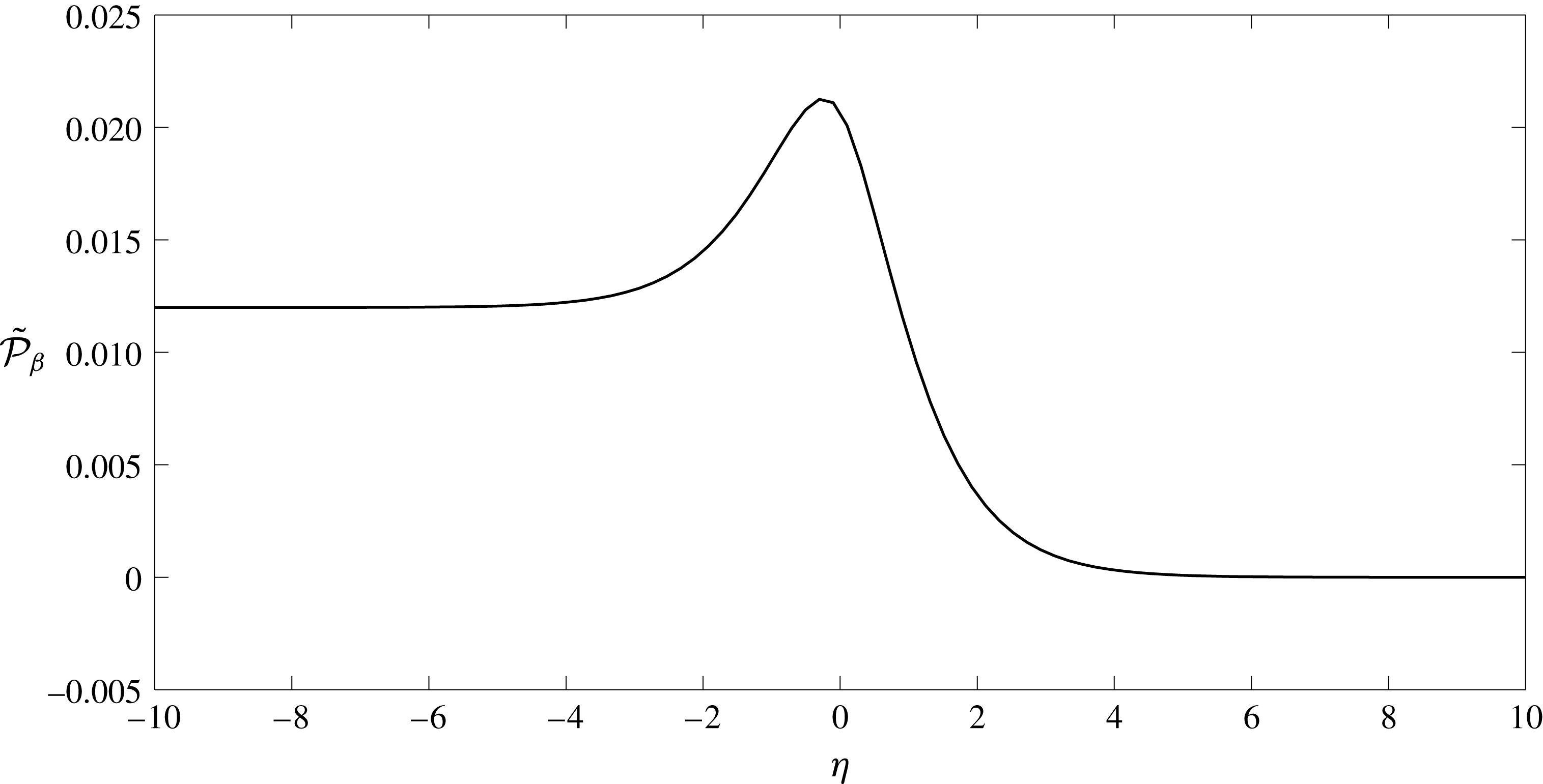
Let us explore a traction vector exerted on the interface. A stress tensor within the Debye layer has the form
 $\tilde{\unicode[STIX]{x1D70E}}_{\unicode[STIX]{x1D6FD}11}^{(0)}=-\tilde{p}_{\unicode[STIX]{x1D6FD}}^{(0)}+2V_{\unicode[STIX]{x1D6FD}}^{\prime }(\unicode[STIX]{x1D709})$
,
 $\tilde{\unicode[STIX]{x1D70E}}_{\unicode[STIX]{x1D6FD}12}^{(0)}=\tilde{\unicode[STIX]{x1D70E}}_{\unicode[STIX]{x1D6FD}21}^{(0)}=0$
,
 $\tilde{\unicode[STIX]{x1D70E}}_{\unicode[STIX]{x1D6FD}22}^{(0)}=-\tilde{p}_{\unicode[STIX]{x1D6FD}}^{(0)}-2V_{\unicode[STIX]{x1D6FD}}^{\prime }(\unicode[STIX]{x1D709})$
, so the traction vector has components
 $\tilde{t}_{\unicode[STIX]{x1D6FD}1}^{(0)}=\tilde{\unicode[STIX]{x1D70E}}_{\unicode[STIX]{x1D6FD}11}^{(0)}n_{1}+\tilde{\unicode[STIX]{x1D70E}}_{\unicode[STIX]{x1D6FD}12}^{(0)}n_{2}$
,
 $\tilde{t}_{\unicode[STIX]{x1D6FD}2}^{(0)}=\tilde{\unicode[STIX]{x1D70E}}_{\unicode[STIX]{x1D6FD}12}^{(0)}n_{1}+\tilde{\unicode[STIX]{x1D70E}}_{\unicode[STIX]{x1D6FD}22}^{(0)}n_{2}$
where
 $\boldsymbol{n}=(n_{1},n_{2})$
is a normal at the interface. We conclude that the traction vector undergoes a jump due to a jump in pressure, so
 $[\boldsymbol{t}_{\unicode[STIX]{x1D6FD}}^{(0)}]=-[p_{\unicode[STIX]{x1D6FD}}^{(0)}\boldsymbol{n}]$
.
 $$\begin{eqnarray}\displaystyle & & \displaystyle c_{lh}^{(1)}=c_{fh}^{(1)},\quad \unicode[STIX]{x1D711}_{lh}^{(1)}=\unicode[STIX]{x1D711}_{fh}^{(1)},\end{eqnarray}$$
and non-homogeneous components
 $$\begin{eqnarray}\displaystyle & \displaystyle c_{\unicode[STIX]{x1D6FD}p}^{(1)}=-A_{\unicode[STIX]{x1D6FD}c}\frac{\unicode[STIX]{x2202}(\boldsymbol{v}_{\unicode[STIX]{x1D6FD}}^{(0)}\boldsymbol{\cdot }\unicode[STIX]{x1D749})}{\unicode[STIX]{x2202}\unicode[STIX]{x1D70F}}, & \displaystyle\end{eqnarray}$$
 $$\begin{eqnarray}\displaystyle & \displaystyle \unicode[STIX]{x1D711}_{\unicode[STIX]{x1D6FD}p}^{(1)}=-A_{\unicode[STIX]{x1D6FD}\unicode[STIX]{x1D711}}\frac{\unicode[STIX]{x2202}(\boldsymbol{v}_{\unicode[STIX]{x1D6FD}}^{(0)}\boldsymbol{\cdot }\unicode[STIX]{x1D749})}{\unicode[STIX]{x2202}\unicode[STIX]{x1D70F}}, & \displaystyle\end{eqnarray}$$
 $$\begin{eqnarray}\displaystyle & \displaystyle \boldsymbol{v}_{l}^{(0)}=\unicode[STIX]{x1D719}_{f}\boldsymbol{v}_{f}^{(0)},\quad \unicode[STIX]{x1D748}_{l}^{(0)}\boldsymbol{\cdot }\boldsymbol{n}=\unicode[STIX]{x1D748}_{f}^{(0)}\boldsymbol{\cdot }\boldsymbol{n}-A_{p}\frac{\unicode[STIX]{x2202}(\boldsymbol{v}_{f}^{(0)}\boldsymbol{\cdot }\unicode[STIX]{x1D749})}{\unicode[STIX]{x2202}\unicode[STIX]{x1D70F}}\boldsymbol{n}, & \displaystyle\end{eqnarray}$$
where
 $\unicode[STIX]{x1D749}$
is a local tangent vector.
Appendix C. Flow scalings in the Debye layer
Let us suppose the scalings given by (B 2), with the exception that we will suppose that there is an
 $O(1)$
vertical flow
 $v_{2}=\bar{v}_{2}^{(0)}+\cdots \,$
. Continuity at
 $O(1/\unicode[STIX]{x1D6FF})$
tells us that
 $\bar{v}_{2}^{(0)}$
must therefore be constant through the layer, i.e.
 $\bar{v}_{2}^{(0)}(\unicode[STIX]{x1D709},\unicode[STIX]{x1D702})=\bar{v}_{2}^{(0)}(\unicode[STIX]{x1D709})$
. The inner ionic vertical fluxes at
 $O(1)$
would also be given by
 $$\begin{eqnarray}\displaystyle \bar{J}_{\pm }^{(0)}=\unicode[STIX]{x1D6FE}_{\pm }\bar{c}_{\pm }^{(0)}\bar{v}_{2}^{(0)}-\frac{\text{d}\bar{c}_{\pm }^{(1)}}{\text{d}\unicode[STIX]{x1D702}}\mp \bar{c}_{\pm }^{(0)}\frac{\text{d}\bar{\unicode[STIX]{x1D711}}^{(1)}}{\text{d}\unicode[STIX]{x1D702}}\mp \bar{c}_{\pm }^{(1)}\frac{\text{d}\bar{\unicode[STIX]{x1D711}}^{(0)}}{\text{d}\unicode[STIX]{x1D702}}=A_{\pm }, & & \displaystyle\end{eqnarray}$$
where
 $A_{\pm }$
is a constant since the Nernst–Planck transport equation at
 $O(1/\unicode[STIX]{x1D6FF})$
tells us that
 $\unicode[STIX]{x2202}_{\unicode[STIX]{x1D702}}\bar{J}_{\pm }^{(0)}=0$
(the argument here remains the same whether the variables above are those in the lumen, or the EGL). These inner fluxes must match to the vertical
 $O(1)$
fluxes in the bulk lumen/EGL which, by virtue of the fact that the zeroth-order ion concentrations and potential are constant, are given by
 $$\begin{eqnarray}\displaystyle J_{\pm }^{(0)}=\unicode[STIX]{x1D6FE}_{\pm }c_{\pm }^{(0)}v_{2}^{(0)}. & & \displaystyle\end{eqnarray}$$
Since
 $\bar{c}_{\pm }^{(0)}$
and
 $\bar{\unicode[STIX]{x1D711}}^{(0)}$
must match to their counterparts in the bulk lumen/EGL in their own right
 $$\begin{eqnarray}\displaystyle & \displaystyle -\frac{\text{d}\bar{c}_{\pm }^{(1)}}{\text{d}\unicode[STIX]{x1D702}}\mp \bar{c}_{\pm }^{(0)}\frac{\text{d}\bar{\unicode[STIX]{x1D711}}^{(1)}}{\text{d}\unicode[STIX]{x1D702}}\mp \bar{c}_{\pm }^{(1)}\frac{\text{d}\bar{\unicode[STIX]{x1D711}}^{(0)}}{\text{d}\unicode[STIX]{x1D702}}\rightarrow 0, & \displaystyle\end{eqnarray}$$
and
 $$\begin{eqnarray}\displaystyle & \displaystyle \bar{c}_{\pm }^{(0)}\rightarrow A_{\pm }/(\unicode[STIX]{x1D6FE}_{\pm }\bar{v}_{2}^{(0)}) & \displaystyle\end{eqnarray}$$
as
 $\unicode[STIX]{x1D702}\rightarrow \pm \infty$
. However,
 $\bar{v}_{2}^{(0)}$
is constant through the Debye layer, with the result that both
 $\bar{c}^{(0)}$
and
 $\bar{c}_{+}^{(0)}$
would not jump across the Debye layer. This would imply the same constant ion concentrations in both the bulk lumen/EGL, which is not compatible with the bulk electroneutrality conditions at zeroth order (3.9). Hence we deduce that there can be no
 $O(1)$
vertical flow through the Debye layer.