1 Introduction
Textual entailment recognition asks the question whether a piece of text like
The Cassini Spacecraft has taken images from July 22, 2006 that show rivers and lakes present on Saturn's moon Titan.
implies a hypothesis like
The Cassini Spacecraft reached Titan.
There exist many interesting approaches to this problem (see Dagan, Glickman and Magnini Reference Dagan, Glickman and Magnini2005; Bar-Haim et al. Reference Bar-Haim, Dagan, Dolan, Ferro, Giampiccolo, Magnini and Szpektor2006; Giampiccolo et al. Reference Giampiccolo, Magnini, Dagan, Dolan and Pantel2007) for various recent efforts. This paper will present a work that models the probability of entailment in terms of ideas motivated by approaches like the edit distance (Kouylekov and Magnini Reference Kouylekov, Magnini, Dagan, Glickman and Magnini2005, 2006; Adams Reference Adams, Bar-Haim, Dagan, Dolan, Ferro, Giampiccolo, Magnini and Szpektor2006; Tatu et al. Reference Tatu, Iles, Slavick, Novischi, Moldovan, Bar-Haim, Dagan, Dolan, Ferro, Giampiccolo, Magnini and Szpektor2006; Bar-Haim et al. 2007; Iftene and Balahur-Dobrescu Reference Iftene, Balahur-Dobrescu, Giampiccolo, Magnini, Dagan, Dolan and Pantel2007). However, instead of defining some distance based on edits, we will generate derivations in some calculus that is able to transform dependency parse trees. The special property of our calculus is that the truth is only preserved with a certain probability along its derivations. This might sound like a disadvantage. However, in commonsense reasoning there is usually a lot of uncertainty due to the fact that it is impossible to formalize all world knowledge. We think that probabilities might help us in such situations in which it is impossible to include everything into the model but in which nonetheless we want to do reasoning. The main idea of this paper can be formulated as follows: Model the probability of entailment as the maximally achievable probability of preserving the truth along derivations in some probabilistically sound calculus.
Let us further explain this idea: we are considering calculi that can transform given text into hypotheses. These mechanisms should be designed to preserve the truth along their derivations. However, we believe that in practice such calculi will always remain imperfect due to the difficulty of correctly formalizing commonsense reasoning. Because of this we do not restrict ourselves to sound calculi but instead consider probabilistically sound calculi. For such calculi we estimate the probability of preserving the truth for each possible atomic transformation of the calculus. This allows us to assign a probability to each derivation in the calculus simply by multiplying all probabilities of preserving the truth along the derivation. In theory, we can consider for given text/hypothesis pairs all possible derivations, each having a certain probability of preserving the truth. If we can find a derivation for a text/hypothesis pair that achieves a large probability of preserving the truth, e.g. because it is short or because it only uses transformations that are known to preserve the truth with high probability, it is reasonable to believe that the text does imply the hypothesis; i.e. the text entails the hypothesis with large probability. In most calculi we can usually also construct many valid derivations that could be arbitrarily long and thus might only achieve arbitrarily small probabilities. To ignore those other derivations, we propose to define the probability of entailment as the maximally achievable probability of preserving the truth along some derivation in some fixed calculus as will be detailed in the following.
2 Defining the probability of entailment
First of all, let us assume that the text and the hypothesis of a textual entailment example are represented as dependency trees T and H. We would like to formalize the probability that T entails H, more precisely the probability of the event that T entails H. We denote this event by T ⊧ H using the entailment relation. The probabilities of such events are parameterized by a vector θ; i.e. each parameter vector θ provides us probabilities pθ(T ⊧ H) for all events of the form T ⊧ H. In order to define pθ(T ⊧ H) we first introduce the probability of preserving truth along syntactic derivations in some calculus which we introduce next.
Suppose we are given n transformations TF1,. . . , TFn that are designed to modify dependency trees. We call a tuple of such transformations a derivation, which we denote by τ with length ℓ(τ). Let τj count the number of times TFj appears in τ. Furthermore, let τ(T) be the result of applying the transformations in τ to some dependency tree T; e.g. for τ = (TF3, TF3, TF17) with ℓ(τ) = 3 we have τ(T) = TF17(TF3(TF3(T))). For a derivation τ with τ(T) = H we denote by T ⊢τH the event that the derivation τ preserves the truth. Thus τ(T) = H does not always imply T ⊢τH. Next we will model the probability of that event.
For each given transformation TFj, the probability of preserving truth is modelled as a constant value θj independent of the dependency tree T it is applied to, i.e.

with parameter θ being the vector of all θj. The idea is that applying a transformation to T could also create a dependency tree that is sometimes not entailed by T anymore. Consider e.g. the transformation that extracts an appositive and adds a new sentence for it. Usually this is correct, but there are situations in which the appositive appears inside a quote, where it might lead to a wrong conclusion. Thus it makes sense to consider probabilities to deal with imperfect calculi.
Suppose that a derivation τ = (t 1,. . ., t ℓ(τ) derives H from T, i.e. τ(T) = H. Then we define the probability of preserving the truth along the derivation τ, i.e. of the event T ⊢τH, as the product of the preservation probabilities of the transformations involved:

with T 1 = T, Ti +1 = ti(Ti) and T ℓ(τ) = H. Note that even though for a certain dependency tree T applying different derivations τ and σ can result in the same tree, i.e. τ(T) = σ(T), their probabilities of preserving truth can be different, since the probabilities depend on the transformations applied. With other words the events T ⊢τH and T ⊢σH are different events if τ ≠ σ and thus get usually different probabilities assigned. For example consider a derivation that performs unnecessary steps. Even though it reaches the same result as a more succinct derivation, its probability of preserving truth can be expected to be smaller. In other words, the probability of preserving the truth is a property of a derivation and not a property of a pair of dependency trees.
In the previous paragraphs we have defined probabilities of preserving truth for all finite-length derivations in the calculus. This allows us now to define the probability of T ⊧ H to be the maximal probability over all possible derivations,

In other words, the probability of entailment is the largest achievable probability of preserving the truth along all possible derivations.Footnote 1
In the following we introduce a set of transformations that is able to transform any text into any hypothesis, and we will propose a heuristic that generates such derivations.
3 Heuristically generating derivations
After explaining the preprocessing and parsing steps, we will describe the set of transformations and our heuristic to generate derivations in the induced calculus. Then we explain how to learn the parameters of our model and how to employ them to classify unseen test examples. Finally, we point out a connection between our procedure and logistic regression which will be applied for comparison to the feature vectors computed by our calculus.
3.1 Preprocessing and parsing
For preprocessing we apply the following steps to the text string and the hypothesis string:
(1) Remove white space, dots and quotation marks at beginning and end.
(2) Remove trailing points of abbreviations.
(3) Remove space between names, e.g. ‘Pat Smith’ becomes ‘PatSmith’.
(4) Unify numbers, e.g. resolve ‘million’.
(5) Unify dates, e.g. ‘5 June’ becomes ‘June 5’.
We then split the text string into sentences simply by splitting at all locations containing a dot followed by a space. The resulting strings are fed to the Stanford Parser (Klein and Manning Reference Klein and Manning2003; de Marneffe, MacCartney and Manning Reference de Marneffe, MacCartney and Manning2006) with its included pretrained model and options ‘-retainTmpSubcategories’ and ‘-splitTMP 1’. This allows us to generate dependency trees the nodes of which contain a single stemmed word, its part-of-speech tag and its dependency tag (as produced using the parser's output options ‘wordsAndTags’ and ‘typedDependencies’; see de Marneffe et al. Reference de Marneffe, MacCartney and Manning2006). For the stemming we apply the function ‘morphy’ of the NLTK-LITE toolbox (Bird Reference Bird2005). If the text string contains more than one sentence, they will be combined into a single dependency tree with a common root node. Let us from now on refer to the dependency trees of text and hypothesis by T and H.
3.2 Generating derivationstitle
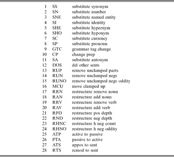
The heuristic described in the following generates a derivation that transforms T into H. For brevity we will use in the text the abbreviations of the transformations as listed in Table 1.
All transformations with their abbreviations.

(1) Resolve appositives and relative clauses. All derivations for some T and H start by converting all existing appositives and relative clauses in T to new sentences that are added to T. For each appositive or relative clause that was resolved in this step, the applied transformation, ATS or RTS, is appended to τ. For instance for the sentence ‘Alice, the sister of Bob, likes hiking’ the transformation ATS will generate the sentences ‘Alice likes hiking’, ‘The sister of Bob likes hiking’ and ‘Alice is the sister of Bob’.
(2) Calculate how H can clamp to T. Often there are several possibilities to assign all or some of the words in H to words in T. For simplicity our system currently ignores certain grammatical parts which are auxiliaries (‘aux’), determiners (‘det’), prepositions (‘prep’) and possessives (‘poss’). Furthermore, we currently ignore words of those parts of speech (POS) that are not verbs (‘VB’), nouns (‘NN’), adjectives (‘JJ’), adverbs (‘RB’), pronouns (‘PR’), cardinals (‘CD’) or dollar signs (‘$’). For all other words wH in H and words wT in T we calculate whether wT can be substituted by wH. For this we employ amongst simple heuristics also WordNet 2.1 (Fellbaum Reference Fellbaum1998) as described next:
(i) Are the tokens and POS tags of wT and wH identical? If yes, return (1, ‘identity’).
(ii) If the POS tags of wT and wH indicate that both words appear in WordNet continue with (iii), otherwise with (viii).
(iii) Are they antonyms in WordNet? If yes, return (2, ‘antonym’).
(iv) Are they synonyms in WordNet? If yes, return (2, ‘synonym’).
(v) Does wH appear in the hypernym hierarchy of wT in WordNet? If yes, return (z, ‘hyponym’) with z being the distance; i.e. wT is a hyponym of wH.
(vi) Does wT appear in the hypernym hierarchy of wH in WordNet? If yes, return (z, ‘hypernym’) with z being the distance; i.e. wT is a hypernym of wH
(vii) Are they named entities that share certain parts of their strings? If yes, return (z, ‘named entity’) with z being larger dependent on how different they are.
(viii) Is wT a pronoun and wH a noun? If yes, return (2, ‘pronoun’).
(ix) Are wT and wH exactly matching cardinals? If yes, return (1, ‘number’).
(x) Are wT and wH identical currencies? If yes, return (1, ‘currency’).
(xi) Are wT and wH both currencies? If yes, return (2, ‘currency’).
Note that along the hierarchy in WordNet we also look one step along the ‘derived form’ pointer to allow a noun like ‘winner’ to be substitutable by the verb ‘win’. If a word wT is substitutable by a word wH, we say that wT and wH are clamped. We call the whole assignment that assigns some or all words of H to words in T a clamp. Since usually a single word wH is clamped to several words in T, we will often have several different clamps. For example if H has three words each of which is clamped to four words in T there are five possibilities for each of the three words: either clamp one of the four possible words in T or omit the clamp. Thus we obtain 5⋅ 5⋅ 5 clamps in total (including the completely empty clamp), i.e. 125 possible ways to clamp the words in H to words in T.
Each of these different clamps gives rise to a different derivation. Thus for lengthy text/hypothesis the number of possible clamps explodes exponentially, posing a serious search problem. For now, we have circumvented this problem by limiting the possible number of clamps considered. Let us for simplicity continue to focus on a single clamp and see how to complete a single derivation τ.
(3) Substitute the clamped words. If wH and wT are clamped, we know what their relationship is; e.g. (3, hypernym) means that we have to go three steps up wH's hypernym hierarchy in WordNet to reach wT. Thus we have to apply three times the transformation SHE to substitute wT by wH, which we reflect in τ by appending three times SHE to it. Similarly, we add other transformations (which could be SS, SN, SNE, SI, SHO, SC, SP, SA) for other relations. Additionally, the substitution of wT with wH might also trigger other transformations, such as PTA, ATP, CP and GTC, which try to adjust the surrounding grammatical structure. All applied transformations will be appended to the derivation τ.
(4) Pick the sentence with the most clamps. After substituting all clamped words, we simply pick the sentence in T with the most clamped words and delete the others using DOS. For example if T consists of three sentences, after this step T will only contain the single sentence with the most clamps and DOS will be appended twice to τ.
(5) Remove subtrees that do not contain clamped nodes. After this step we add for each removed node the transformation RUP to τ. Then we add RUN for each removed negation modifier (‘neg’) and additionally RUNO if the number of removed negation is odd. RUNO is a somewhat artificial transformation and acts more like a flag. This might be changed in future sets of transformation to better comply with the transformation metaphor.
(6) Move the clamped nodes closer to the root and remove unclamped subtree.} Again we do some counting before and after this step, which determines the transformations to add to τ. In particular we count how many verbs are passed by moving clamped nodes up. For each passed verb we add MCU to τ.
(7) Restructure and add the missing pieces. The definition in (3) requires that any T can be transformed into any H; otherwise the maximum is undefined. In the last step we will thus remove all words in T which are not needed for H and add all missing words to T and restructure until T becomes H. For the bookkeeping we count the number of nouns, verbs and negation modifiers that have to be added and removed. Furthermore, we count how many levels up or down we need to move words in T such that they match the structure in H. For all these countings we add accordingly as many transformations, RRN, RRV, RAN, RAV, RPD, RND, RHNC, RHNO (see Table 1 for short explanations). In other words, we measure how different T and H are after step (6). In practice the latter transformations are not really executed, but we simply count how often we would have to apply them.
Finally, the completed derivation τ with τ(T) = H is converted to a n-dimensional feature vector [τ1,. . ., τn]⊤ with τj being (as defined in Section 2) the number of times the jth transformation from Table 1 appears in τ. As a simple example consider the text
Kiwis, who are chased by opossums, eat small invertebrates, seeds, grubs, and many varieties of worms.
and the hypothesis
Opossums chase birds.
The derivation of the dependency tree H of the hypothesis from the dependency tree T of the text is illustrated in Figure 1 and explained in the following: In step (1) the relative clause ‘who are chased by opossums’ is converted into a new sentence using ‘Kiwis’ as the subject by transformation RTS (‘rcmod to sent’). Step (2) finds possible clamps between text and hypothesis. A possible clamp is that ‘Kiwis’ matches hypernym ‘birds’ and that ‘chase’ and ‘opossum’ in the newly added sentence in T matches ‘chase’ and ‘opossum’ in the hypothesis. Next in step (3) we substitute the clamped ‘Kiwis’ by its hypernym ‘birds’ by transformation SHE (‘substitute hypernym’). Also we change passive to active in that newly added sentence by transformation PTA (‘passive to active’). Step (4) picks the newly added sentence, since it has the most clamps, and removes the other sentence by transformation DOS (‘delete other sentences’). Steps (5) through (7) do nothing in this example, since we already reached the hypothesis in step (4).
Toy example derivation: the text is ‘Kiwis, who are chased by opossums, eat small invertebrates, seeds, grubs, and many varieties of worms’ and the hypothesis is ‘Opossums chase birds’. The length-four derivation τ = (SHE, RTS, PTA, DOS) transforms the dependency tree T into H.

Note that this example generates a single derivation. Since in step (2) there are other clamps possible, our heuristic generates also derivations for each of the other clamps. However, wrong clamps lead of course to more complicated derivations. More concretely, they would require much more restructuring in steps (5)–(7). In practice we limit the maximal number of clamps in step (2) which can become very large for longer texts and hypothesis.
One further caveat is as follows: the just presented heuristic to find derivations and the set of considered transformations is by no means designed to be optimal. Instead it should be merely seen as a vehicle to present a concrete worked-out example of our probabilistic approach. See Section 5 for more thoughts on this.
3.3 Estimating the parameters
Let Dtr = {(T 1, H 1, y 1),. . ., (Tm, Hm, ym)} be the m training examples with yi ∈ {0, 1} indicating entailment. For brevity we define

to abbreviate the probability of entailment modelled as outlined in Section 2. Then the data likelihood can be written as
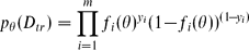
We would like to maximize p θ(Dtr) with respect to the vector θ. However, this optimization is difficult to perform, since each fi is a maximum over all possible derivations from Ti to Hi (see (3)). In order to approximate it we choose the following way:
(i) Generate for each example pair several derivations (as described in the previous section), and choose the d shortest ones for some fixed number d. We choose d = 8 in the experiments. For pairs which do not induce d different derivations, simply copy the shortest derivations of the existing ones to get d derivations (some of which will in that case be identical). The reason for this is to ensure equal influence of each training example.
(ii) There are now d ⋅ m derivations in total. We denote the corresponding feature vectors by x 1,. . ., xd⋅m. Note that xi is a vector containing the countings of the different transformations. For example if the corresponding derivation is τ, then xij = τj.
(iii) Similarly copy the training labels yi to match those d ⋅ m feature vectors; i.e. now our data becomes Dtr = (x 1, y 1),. . ., (xd⋅m, yd⋅m).
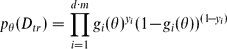
(vi) Replacing fi(θ) by
(6)the data likelihood becomes (7)
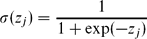
(v) Replace furthermore each θj by
(8)with σ being the sigmoidal function, which ensures that the values for θj stay between zero and one.(vi) Maximize pz(Dtr) in terms of z = [z 1,. . ., z n]⊤ using gradient ascent.
(vii) Calculate θj = σ(zj) for all j.

Note that each text/hypothesis pair (Ti, Hi) generates d = 8 data points x d⋅(i−1)+ 1,. . . , xd⋅i. On the other hand, our definition of the entailment probability (see (3)) suggests that only the single shortest derivation as a training case should be used. This is of course the preferred procedure if there are enough training pairs available. However, in our experiments with only a few hundred training pairs, we found out that taking the d = 8 shortest derivations provides valuable data that improves the overall performance. Also our definition suggests that the derivation which is shortest with respect to the current parameter setting should be used. This implies some alternating scheme: Initialize θ randomly or somewhat informed (e.g. by a first run). Then use θ to find the shortest derivation with respect to the current parameter setting θ and repeat until convergence of θ. We tried such an alternating scheme and observed inferior performance; thus we used the simpler approach outlined above.
3.4 Classifying the test data
Having estimated the parameter vector θ we can apply the trained model to the test data Dte to infer its unknown labels. Since we only generate some derivations and cannot try all possible – as would be required by (3) – we again transform the test data into d ⋅ n feature vectors x 1,. . ., x d⋅n, hereby assuming that we have n test examples. Note that x d⋅(i−1)+1},. . ., xd⋅i are the d generated feature vectors belonging to the ith test example (Ti, Hi). To approximate the probability of entailment we take the maximum over the d feature vectors assigned to each test example; e.g. for (Ti, Hi), this becomes

The class label and the answer to the question whether Ti entails Hi is obtained by checking whether p θ(Ti⊧ Hi) is greater than or equal to 0.5. Note that since we can only consider some derivations and not all of them, our approximation provides a lower bound on the probability of entailment as defined in (3).
This completes the description of the system based on a probabilistically sound calculus.
3.5 Logistic regression
Taking the logarithm of (3), we obtain

We see that the log-probability of entailment for each pair can be calculated by an inner product between the feature vector and the component-wise logarithm of θ.
Note that logθj is always negative (since θj ≤ 1). If we omit this restriction and replace logθj by a real-valued weight wj, we are no longer guaranteed that that the inner product of the feature vector τ and w is a log-probability. However, after applying the sigmoidal function (see (8)), we obtain a number between zero and one which can be directly interpreted as a probability:
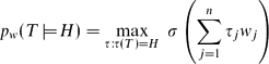
Ignoring the maximum, this model is exactly the logistic regression model, for which we have just shown that it is closely related to our model.Footnote 2
4 Evaluating the method
We will compare the results of the probabilistic calculus with logistic regression on the feature vectors generated by the heuristic. Also for logistic regression we use the approximation for the maximum in (11) analogous to (9). We will see that we have comparable performance. However, as we will discuss in Section 4.3, the weight vector of logistic regression has a different interpretation than the model parameters of the probabilistic calculus.
4.1 RTE2 and RTE3
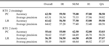
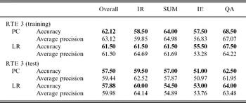
Tables 2 and 3 show the performance of the probabilistic calculus and logistic regression on the datasets from the second and third PASCAL Challenge on Recognizing Textual Entailment (see Bar-Haim et al. Reference Bar-Haim, Dagan, Dolan, Ferro, Giampiccolo, Magnini and Szpektor2006; Giampiccolo et al. Reference Giampiccolo, Magnini, Dagan, Dolan and Pantel2007). Shown are the accuracies (in boldface) and the average precision (in normal font) for probabilistic calculus and logistic regression overall and distinguished for the different subtasks. The first fact we see from the results is that the probabilistic calculus system is better than random. However, with 55.64% (RTE2) and 57.50% (RTE3) it is not much better. Applying logistic regression to the same feature vectors leads to similar results, which shows that the feature vectors give some hint about entailment but are clearly not yet sufficient, with accuracies 56.39% (RTE3) and 57.88% (RTE3).
Results of the RTE2 data. Shown are the accuracies on the training and test sets. Results marked with ‘PC’ show performance for the probabilistic calculus and results marked with ‘LR’ for logistic regression. The boldface numbers are accuracies; the normal-font numbers are average-precision scores.

Results of the RTE3 data. Shown are the accuracies on the training and test sets. Results marked with ‘PC’ show performance for the probabilistic calculus and results marked with ‘LR’ for logistic regression. The boldface numbers are accuracies; the normal-font numbers are average-precision scores.

Examining the task-specific data, we see that our features completely fail for the information extraction (IE) subtask. However, we obtain good results, well above 60% in some of the subtasks. We also note that the accuracies of the training data are much better than the accuracies of the test data, which indicates that there was possibly some overfitting.
Comparing the task-specific results between the RTE2 and RTE3 datasets, it is curious that in RTE2 the summarization (SUM) task was the easiest, while in RTE3 it was the question answering (QA) task. This is probably due to changes in the data generation process.
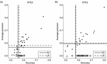
To compare the performance of our system with the current state-of-the-art systems we present in Figure 2 the results of all submissions to the RTE2 and RTE3 challenge (see Bar-Haim et al. Reference Bar-Haim, Dagan, Dolan, Ferro, Giampiccolo, Magnini and Szpektor2006; Giampiccolo et al. Reference Giampiccolo, Magnini, Dagan, Dolan and Pantel2007). Trained and evaluated on the RTE2 data, our method performs better than some of the approaches, but worse than most methods. Trained and evaluated on the RTE3 data, our method shows below the current state-of-the-art performance. Overall, it seems that the RTE3 data was somewhat simpler to deal with than the RTE2 data.
Comparison against the test performance of all other (a) RTE2 and (b) RTE3 submissions. Each cross and each circle (results without precision) corresponds to one submission to these challenges. Lower left is bad; upper right is good.

What are the possible reasons that our system did not compete well against the other approaches? We believe that the basic idea of our system to define probabilities of entailments in terms of derivations in some probabilistically sound calculus is a promising approach to the textual entailment problem. However, the current set of transformations as presented in this paper is too simplistic compared to the processing done by other methods that performed very well in the RTE3 challenge (such as Hickl and Bensley Reference Hickl, Bensley, Giampiccolo, Magnini, Dagan, Dolan and Pantel2007; Tatu and Moldovan Reference Tatu, Moldovan, Giampiccolo, Magnini, Dagan, Dolan and Pantel2007). As was also suggested by one of the reviewers, we believe that our performance could be improved by a better calculus that takes into account and implements the latest findings in linguistic semantics.
4.2 Long versus short
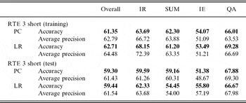
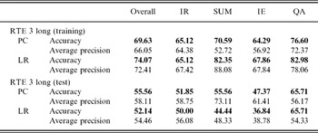
The RTE3 data had some examples which contained an especially long text part. Tables 4 and 5 allow us to examine our system with respect to longer or shorter texts. For this we trained our model either only on the short examples (see Table 4) or only on the long examples (see Table 5). Comparing the results we see that our approach had especially problems with the longer texts. On the other hand it did particularly well on the short examples (almost 60% accuracy).
Results of the short examples of the RTE3 data. Shown are the accuracies on the training and test sets. Results marked with ‘PC’ show performance for the probabilistic calculus, results marked with ‘LR’ for logistic regression. The boldface numbers are accuracies; the normal-font numbers are average-precision scores.

Results of the long examples of the RTE3 data. Shown are the accuracies on the training and test sets. Results marked with ‘PC’ show performance for the probabilistic calculus, results marked with ‘LR’ for logistic regression. The boldface numbers are accuracies; the normal-font numbers are average-precision scores.

Of course, these estimates of the accuracies are not precise due to small dataset size. (Tables 9 and 10 list the number of data points corresponding to the entries in the other tables.)
4.3 Interpreting the model parameters
Even though the performance of our system is not yet competitive with the state-of-the-art textual entailment systems, the model parameters are interesting to analyze. Of course, due to the small size of the dataset the parameters are only coarsely estimated. Thus the following discussion should be taken with a grain of salt. Nonetheless we believe that it is illustrating how the model parameters can be interpreted.
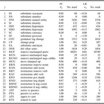
Table 6 contains all possible transformations of the calculus we used in this paper. In the last columns we list the model parameters θj for the probabilistic calculus and the weight parameters wj for the logistic regression that were estimated using the RTE3 data. Additionally we list how often that particular derivation was used in the derivation of examples of the RTE3 dataset. Note that the two ‘usage’ columns slightly differ for probabilistic calculus and logistic regression, since when approximating the maxima in (9) and (11) different derivations might have been chosen.
The weight vectors for the probabilistic calculus (PC) and logistic regression (LR). See the text for discussion.

Number of training (Tr) and testing (Te) points overall and for the different subtasks in the RTE2 data. Note that two examples were excluded, since the applied parser was not able to produce any parse tree for those.

Number of training (Tr) and testing (Te) points overall and for the different subtasks in the RTE3 data.

Number of training (Tr) and testing (Te) points overall and for the different subtasks in the RTE3 data that were declared to have short text.

Number of training (Tr) and testing (Te) points overall and for the different subtasks in the RTE3 data that were declared to have long text.

First of all note that for derivations that were never used, the model parameter θj is 0.5 and wj is zero. This corresponds to the initialization of the optimization procedures.
In the case in which θj = 1.0 we learn about the corresponding transformation that its application to the text does not change its truth value. This is reasonable for changing active to passive (ATP), but not so much for changing a preposition (CP). The reason that also θ25 is 1.0 is probably that this transformation appeared in derivations of entailed and also of not-entailed examples. Thus observing the application of CP does not tell us anything about the final outcome.
The difference between the model parameters of probabilistic calculus and logistic regression is that the values of θj can only decrease the likelihood of entailment, since θj ≤ 1, while wj (corresponding to the logarithm of θj) can be positive as well, which means that applying ATP with w 25 = 0.88 < 0 (and so log w 25 < 1) is increasing the probability of entailment. Of course in the calculus that does not make sense, since each application of a transformation can only lower the probability of entailment. Thus if by chance all passive-to-active (PTA) transformations appear only in derivations of some entailed examples and never in non-entailed examples, the logistic regression model will assign a positive weight. On the other hand in the probabilistic calculus model the corresponding model parameter will be 1.0. This is also the reason for the fact that for almost all transformation for which wj < 0, we have θj = 1.0.
5 Related work
Already Glickman, Dagan and Koppel (Reference Glickman, Dagan and Koppel2005) have proposed a probabilistic approach for textual entailment. Their idea is to assume a generative model for texts and possible worlds, which assign probabilities to all possible hypotheses. Such a model lets us define that text T entails hypothesis H if and only if p(“H is true” |T) < p(“H is true”), i.e. if and only if knowing the text increases the probability of the hypothesis to be true. In practice it is hard to estimate such generative models, and thus in their paper they apply this idea to the subtask of lexical entailment. Nonetheless it is interesting how their generative approach conceptually compares to ours. Informally, (1) can be informally rewritten as

The main difference from Glickman et al. (Reference Glickman, Dagan and Koppel2005) is that we do not need a generative model of the text. Instead our model simplifies the situation by assuming the probability of preserving the truth to depend only on the transformation TFj and not on the text T to be transformed. The entailment relation between T and H is captured by possible derivations, each of which has a certain probability of preserving the truth. Thus instead of employing a generative model we model the relationship between T and H. The relationship between the work of Glickman et al. (Reference Glickman, Dagan and Koppel2005) and our work is remotely similar to the difference between generative and discriminative models for classification problems.
Our work shares also ideas with those of Bar-Haim et al. (Reference Bar-Haim, Dagan, Greental and Shnarch2007a, Reference Bar-Haim, Dagan, Greental, Szpektor, Friedman, Giampiccolo, Magnini, Dagan, Dolan and Pantel2007b) who propose to infer semantic entailment at the lexical–syntactic level. In other words, instead of performing inference in some logical representation, they define a calculus that acts directly on parse trees. Our paper is very much in agreement with their view on this and similarly suggests a calculus on the lexical–syntactic level. (We tried for example transforming dependency trees.) However, while their work puts the focus on the construction of powerful, theoretically grounded rules, our paper puts its emphasis on the idea to probabilistically define the soundness of such rules and to formalize textual entailment in a probabilistic way. We strongly believe that combining their set of syntactic transformations with our probabilistic approach (herewith replacing their approximate matching) would lead to promising results.
Also related to our work is that of Iftene and Balahur-Dobrescu (Reference Iftene, Balahur-Dobrescu, Giampiccolo, Magnini, Dagan, Dolan and Pantel2007) which proposes a transformation-based approach to textual entailment as well, but non-probabilistically. Instead of only transforming the text to reach the hypothesis, as our approach does, they transform the text and the hypothesis until they meet or their remaining edit distance is small. Combining forward search with backward search is probably an efficient way to find good derivations from the text to the hypothesis. This idea and also their set of transformation is in principle also compatible with our probabilistic setting, and it would be interesting to extend their system with our notion of probabilistic soundness.
As one of the reviewers pointed out, how our approach relates to stochastic logic programming (SLP; see Muggleton Reference Muggleton1996) is an interesting question. If we are able to formulate our transformations of the dependency tree calculus as clauses of an SLP, our method will fit very well into SLPs. The probability of preserving the truth for each transformation would then become the probability assigned to the corresponding clause. Possibly we could use the existing SLP machinery to replace our heuristic search procedure to generate derivations by a more principled and efficient method. We believe that this could be a promising direction for future work.
6 Future work and conclusion
This paper introduces a probabilistic approach to textual entailment that is based on a calculus on dependency parse trees. The unique property of our work is that we do not assume soundness for our calculus; instead we only require that its derivations preserve the truth of a statement (in our case of the statement of a dependency tree) with a certain probability depending on the transformations used. This captures the intuition we have about commonsense reasoning in which we sometimes (e.g. due to limited information) can only draw conclusions which are probably correct.
For concreteness we described a heuristic method which generates derivations for text/hypothesis pairs in such a calculus. Given a dataset of examples we explained how the model parameters of the probabilistic calculus can be estimated and applied to unseen data. Furthermore, we discussed the relationship of our approach to logistic regression.
Finally, we showed that the approach works by applying it to datasets from the PASCAL Challenge on Recognizing Textual Entailment. Even though our current results suggest that right now our system might not be able to compete with the state-of-the-art systems for textual entailment we see the potential that our architecture provides a useful platform on which one can test and evolve different sets of transformations on parse trees. Again, we note that such a set of transformations induces a calculus that preserves truth only with a certain probability, which is an interesting concept to follow up. Furthermore, the idea of a probabilistic calculus is not limited to dependency trees but could equally well apply to other representations of text.
Besides working on more powerful and faithful transformations, our system might be improved also simply by replacing our ad hoc solutions for the preprocessing and sentence-splitting. We should also try different parsers and see how they compare for our purposes. Since our approach is based on a probabilistic model, we could also try to incorporate several optional parse trees (as a probabilistic parser might be able to create) with their respective probabilities and create a system that uses probabilities in a consistent way all the way from tagging/parsing to inferring entailment.