1. INTRODUCTION
Future Mars explorations need the vehicles to land precisely at the prescribed locations to complete the missions, such as sample returns, high-mass entry, human explorations and so on. Mars entry phase is the most challenging part of Mars Entry, Descent and Landing (EDL) due to the complex aerodynamics and atmosphere properties (Dutta et al., Reference Dutta, Braun and Karlgaard2014), which make the Mars entry dynamic model strongly nonlinear and time varying. Also, the entire Mars EDL phase only lasts a few minutes. Mars entry phase is also known as the hypersonic phase, which is defined as from the vehicle entering the atmosphere, about 125 km from the surface of Mars with speed around 5,900 m/s, to parachute deployment, and at this time the duration of the vehicle entering into the atmosphere is about 300 seconds. Considering the processing capability of the on board computer, selecting an appropriate navigation filter is of great importance. For nonlinear system state estimations, the most prominent and widely used filter is the Extended Kalman Filter (EKF), which is obtained by first order linearization of the system equations so that the iteration steps of the traditional Kalman filter can be used (Boutayeb and Aubry, Reference Boutayeb and Aubry1999). However, the problem of EKF is that the derivation of the Jacobian matrix is not trivial, and the linearization of the system equations may bring some biases in state estimations. Another commonly used nonlinear filter is the Unscented Kalman Filter (UKF) (Julier et al., Reference Julier, Uhlmann and Durrant-Whyte2000; Julier and Uhlmann, Reference Julier and Uhlmann2004). This kind of filter propagates the mean and covariance of a random variable based on unscented transformation in terms of sigma points. UKF is also called the Sigma Points Kalman Filter (SPKF). Another SPKF is called the Divided Difference Filter (DDF), which uses Stirling's interpolation formula to obtain a second order approximation (Norgaard et al., Reference Norgaard, Poulsen and Ravn2000; Subrahmanya and Shin, Reference Subrahmanya and Shin2009). An advantage of UKF and DDF with EKF is that the computation of the Jacobian matrix can be avoided in the implementations of UKF and DDF, which make them easier in implementation and make savings in the offline computation effort. The limitation of UKF and DDF is that they need Cholesky factorisation of the matrices. In theory, the most accurate filter is the Particle Filter (PF) in which some particles are sampled from the posterior probability density function and then are propagated and weighted based on Bayesian rules (Gordon et al., Reference Gordon, Salmond and Smith1993). The state estimation is the weighted mean of the particles. The price that must be paid for high performance of a PF is computation time (Simon, Reference Simon2006). Considering the characteristics of the filters, it is vital to choose one suitable for Mars entry navigation.
Another difficulty of Mars entry navigation is the lack of measurement devices. During Mars entry, since the vehicle is protected by a heat shield from the aerodynamic heating environment, conventional navigation devices like radar altimetry, Light Directions and Ranging (LIDAR), and optical navigation cameras cannot be used (Crain and Bishop, Reference Crain and Bishop2002). To improve the navigation capability, Mars network-based navigation including Mars orbiters and Mars Surface Beacons (MSBs) has been developed (Li et al., Reference Li, Jiang and Liu2014; Wu et al., Reference Wu, Fu, Xiao and Zhang2014; Li and Peng, Reference Li and Peng2011). However, the Mars orbiter model is built only by simple assumed movement characteristics, which may make the navigation results partial. Lévesque and Lafontaine (Reference Lévesque and Lafontaine2007) developed an innovative navigation scheme for state and parameter estimation. Due to the number limitation of MSBs, Yu et al. (Reference Yu, Cui and Zhu2015) have proposed a method for beacon configuration optimisation based on Lie algebra observability analysis. They made a thorough observability analysis of the navigation system (Yu et al., Reference Yu, Cui and Zhu2014). However, in these works, the measurements from existing Mars orbiters are discarded, which may make the conclusions from these works inapplicable. Another problem of the above works is that Mars rotation is neglected in both dynamic and measurement models and this will result in poor landing precision (Lévesque, Reference Lévesque2006). For example, at equator level, the ground velocity of Mars is
 $v_{M}=\omega_{M} R_{M}=7{\cdot}0882e-5\,\hbox{rad/s}\ast 3397{\cdot}2\,\hbox{km} = 0{\cdot}2408$
km/s, where ω
M
is Mars rotating angular velocity, R
M
is Mars’ radius. In general, Mars entry lasts several minutes, in this paper 300 s, which means that the target landing site at the equator moves about
 $d=v_{M}\hbox{t}= 0{\cdot}2408\,\hbox{km/s}\ast 300\,\hbox{s} = 72{\cdot}24$
km. For future Mars landing accuracy to be within 100 m of the target (Wolf et al., Reference Wolf, Graves, Powell and Johnson2004), Mars rotation must be taken into account. Mars rotation was considered in Kluever (Reference Kluever2008), which evaluated the performance and advantages of Mars entry guidance for Mars precision landing. In Furfaro and Wibben (Reference Furfaro and Wibben2012), Mars rotation was not taken into account, but rather Mars rotation was neglected.
Mars rotation will have an impact on final landing accuracy, not for Mars entry phase precision. However, considering the impact of Mars rotation on landing precision, in Mars entry phase we must consider the Mars entry dynamic and measurement models under Mars rotation. Mars entry phase is the longest period of time, the harshest environment in the EDL. Mars entry navigation technology can not only impact the accuracy of the landing directly, but also determines directly the success of the Mars landing mission.
In this paper, our contributions are that: we have built reasonable dynamic and measurement models for Mars entry navigation considering Mars rotation, based on which we have made a detailed comparison and analysis of the performance of the four nonlinear filters (EKF, UKF, DDF1, PF). Then the theoretical Cramer-Rao Lower Bound (CRLB) of estimation errors are derived to evaluate the performance of the filters. To further verify the filter performance, a consistency test is carried out. Finally, recommendations are given on the selection of the suitable filter in terms of performance and computation costs. The rest of the paper is organised as follows. Section 2 builds a Mars entry dynamic model and measurement model considering Mars rotation. In Section 3, the four types of nonlinear filters are presented. In Section 4, the technical tools including the theoretical CRLB and consistency test are provided. Section 5 provides the simulation results and discussion. Section 6 gives the conclusions.
2. MARS ENTRY DYNAMIC MODEL AND MEASUREMENT MODEL
In this section, the mathematical model describing Mars entry dynamics is presented, which is based on the vehicle only being affected by gravity, atmosphere lift and drag during Mars entry. To build the entry dynamic model and measurement model, the coordinate frames have to be defined first.
2.1. Definitions of Coordinate Frames
(1) Mars Centred Inertial Coordinate Frame (MCICF): denoted by
 ${\bf X}^{i}, {\bf Y}^{i}, {\bf Z}^{i}$
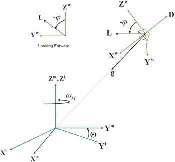
. This frame is depicted in Figure 1, where its origin is centred on Mars, the
 ${\bf X}^{i}$
axis points toward the Martian vernal equinox direction, the
 ${\bf Z}^{i}$
axis points in the direction of the Martian North pole and the
 ${\bf Y}^{i}$
axis completes the right-handed system. The
 ${\bf X}^{i}$
axis and
 ${\bf Y}^{i}$
axis are on the equatorial plane. The MCICF is non-rotating with respect to the stars.
Mars entry vehicle reference frames and lift/drag/bank angle definitions.

(2) Mars centred Fixed Coordinate Frame (MCFCF): denoted by
 ${\bf X}^{m}, {\bf Y}^{m}, {\bf Z}^{m}$
. This frame is similar to the MCICF coordinate frame. The difference is that its
 ${\bf X}^{m}$
axis points in the direction of the Martian prime meridian, and the
 ${\bf Y}^{m}$
axis completes the right-handed system. The MCFCF rotates around Mars along the
 ${\bf Z}^{m}({\bf Z}^{i})$
axis. The rotation angle is Θ which can be calculated by
 $\Theta =\Theta_{0} +\omega_{M} t$
. The coordinate transformation from MCICF to MCFCF is
 $${\bf C}_i^m =\left(\matrix{ \cos \Theta & \sin \Theta & 0 \cr -\sin \Theta & \cos \Theta & 0 \cr 0 & 0 & 1}\right)$$
(3) Wind Coordinate Frame (WCF): denoted by
 ${\bf X}^{w}, {\bf Y}^{w}, {\bf Z}^{w}$
. The unit vectors are expressed as
 ${\bf e}_{1}^{w}$
,
 ${\bf e}_{2}^{w} $
and
 ${\bf e}_{3}^{w}$
, respectively. This frame is defined with respect to the atmosphere, which is depicted in Figure 1. The spacecraft velocity vector relative to the atmosphere in the MCICF is
 $${\bf v}_r = \dot{{\bf r}}-{\bf \omega} \times {\bf r}$$
where
 ${\bf r}$
is the position vector in the MCICF,
 ${\bi \omega} =[0,0,\omega _{M}]^{\rm T}$
is the rotation vector of Mars, “×” is the cross product. The WCF reference vector
 ${\bf e}_{1}^{w} $
is defined as
 $${\bf e}_1^w ={{\bf v}_r \over v_r }$$
where
 $v_{r} =\|{\bf v}_{r}\|$
is the relative velocity magnitude of the vehicle. Since the vectors
 ${\bf e}_{2}^{w} $
and
 ${\bf e}_{3}^{w} $
only need to span the lift space, the right-handed coordinate frame can be formed as below (Tapiero and Bishop, Reference Tapiero and Bishop2013)
 $${\bf e}_2^w =-{{\bf e}_1^w \times {\bf h}\over \| {{\bf e}_1^w \times \hbox{h}} \|}, e_3^w ={\bf e}_1^w \times {\bf e}_2^w$$
where
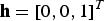 ${\bf h}=[0,0,1]^{T}$
.
From Figure 1, it can be seen that the non-gravity acceleration of the vehicle which is affected by lift and drag is
 $${\bf a}=-D{\bf e}_1^w +L[-{\bf e}_2^w \sin \varphi + {\bf e}_3^w \cos \varphi]$$
where D=| D | and
 $L=\| {\bf L} \|$
are the magnitude of drag and lift respectively and φ is the bank angle. The drag vector is pointing in the opposite direction of the vector
 ${\bf e}_{1}^{w}$
. The lift vector is contained in the (
 ${\bf e}_{2}^{w}$
,
 ${\bf e}_{3}^{w}$
) plane, and its direction can be modulated by the bank angle which is defined as the angle between the lift vector L and
 ${\bf e}_{3}^{w}$
, positive in the clockwise direction when looking in the direction of
 ${\bf e}_{1}^{w}$
.
The expressions of the magnitude of lift and drag are
 $$L={1\over 2}\rho ({\bf r})v_r^2 s/mC_L, D={1\over 2}\rho ({\bf r})v_r^2 s/mC_D$$
where s is the cross-section area of the vehicle, m is the mass, C
L
and C
D
are lift and drag coefficient,
 $\rho ({\bf r})$
is the atmosphere density
 $$\rho ({\bf r})=\rho _0 \exp \left( {{r_0 -\| {\bf r}\|\over h_s }} \right)$$
where ρ0=2e−4 kg/m3 is the nominal reference density, r 0=3437200 m is the reference radius of Mars (40 km above Mars surface), h s =7500 m is the constant scale height.
2.2. Mars entry dynamic model
Based on the definitions of coordinate frames and force analysis above, the dynamic model of the vehicle during Mars entry in MCICF can be built in a general form:
 $$\left\{\eqalign{&{\dot{\bf r}}= {\bf v} \cr & {\dot{\bf v}}={\bf a}+{\bf g}}\right.$$
where
 ${\bf r}=[r_{x} ,r_{y} ,r_{z} ]^{T}$
,
 ${\bf v}=[v_{x} ,v_{y} ,v_{z}]^{T}$
.
 ${\bf g}=-{\mu\over r^{3}}{\bf r}$
is the gravity,
 $\mu =42828{\cdot}29e+9$
m3/s2 is the gravity constant of Mars.
2.3. Mars entry measurement model
Due to the remote distance from Earth, traditional methods used for deep space exploration such as ground-based stations for tracking, observation and communication seem to be unreliable because the communication from ground deep space stations may last several minutes. However, the whole EDL lasts only seven minutes. So, the Mars vehicles have to navigate autonomously. In this paper, the autonomous navigation scheme based on Mars orbiters and MSBs are investigated.
The Curiosity launched by NASA and landed on 5 August 2012 used only two Mars orbiters-MRO and MEX for navigation, which are also adopted as measurements in this paper. With radiometric measurement equipment such as the Electra (Lightsey et al., Reference Lightsey, Mogensen, Burkhart, Ely and Duncan2008) mounted on the vehicle and the orbiters, two-way range measurements can be obtained. According to Wang and Xia (Reference Wang and Xia2015), the movement of the orbiter in polar coordinates can be constructed:
 $$\left\{\eqalign{& r_{ob} ={a(1-e^2)\over 1+ecos(\theta -\bar {\omega })} \cr & r_{ob}^2 \dot {\theta }=\sqrt {\mu a(1-e^2)} }\right.$$
where r
ob
is the distance between the orbiter and the centre of Mars, θ is the angle between the ascending node and the orbiter, a is the semi-major axis of the movement ellipse, e is the eccentricity ratio,
 $\bar {\omega}$
is the argument of perigee and μ is the gravity constant of Mars.
The ecliptic longitude and latitude of the orbiter are
 $$\Omega _{ob} = \left\{ \eqalign{& -\cos ^{-1}\left[ {\cos \theta \over \cos \phi_{ob} }\right] +\Omega , \quad {\phi _{ob} \le 0} \cr & \cos ^{-1}\left[ {\cos \theta \over \cos \phi_{ob} } \right] +\Omega, \quad \quad \phi _{ob} \gt 0} \right.$$
and
 $$\phi _{ob} =\sin ^{-1}\left[ {\sin \theta \sin i\over \sin k} \right]$$
where Ω ob is ecliptic longitude, and Φ ob is the ecliptic latitude, i and k are orbital inclination (angle between longitude and latitude, k=π/2). The relative range measurement between the vehicle and the orbiter can be constructed:
 $$\left\{\eqalign{& R_{ob} =\sqrt {({\bf r}-{\bf r}_{ob} )^T({\bf r}-{\bf r}_{ob} )} \cr & \tilde{R}_{ob} =R_{ob} +\varepsilon _{ob}}\right.$$
where
 $${\bf r}_{ob} =r_{ob} [\matrix{\cos \phi _{ob} & \cos \Omega _{ob} &\cos \phi _{ob} &\sin \Omega _{ob} &\sin \phi _{ob}}]^T$$
 $\varepsilon_{ob}$
is the range measurement noise which is assumed to be zero-mean, and Gaussian white.
The measurement principle from MSB is the same as on the orbiters. The MSB can be pre-deployed by a mission obiter (Pastor et al., Reference Pastor, Bishop, Gay and Striepe2000). The relative range measurement is constructed as below:
 $$\left\{ \eqalign{& \tilde{R}_i =R_i +\varepsilon _R^i ,\quad i=1,\cdots ,N \cr & R_i =\sqrt {(x_B^i -r_x )^2+(y_B^i -r_y )^2+(z_B^i -r_z )^2}} \right.$$
where R
i
refers to the true range from the entry vehicle to the ith beacon,
 ${\tilde{R}_i}$
is the measurement range,
 $x_{B}^{i} $
,
 $y_{B}^{i} $
and
 $z_{B}^{i} $
are the positions of the beacons in MCICF. Considering the rotation of Mars, the position of MSB after time t is
 $$[x_B^i\quad y_B^i\quad z_B^i]^T={\bf C}_i^m [x_B^i (t_0)\quad y_B^i (t_0)\quad z_B^i (t_0 )]^T$$
where
 $[x_{B}^{i} (t_{0})\quad y_{B}^{i} (t_{0})\quad z_{B}^{i} (t_{0} )]$
is the initial position of the beacons,
 ${\bf C}_{i}^{m} $
is the coordinate transform matrix from MCICF to Mars Centred Fixed Coordinate Frame (MCFCF).
To obtain the velocity information directly from the measurements, the relative rate measurements which can be obtained by Doppler shifted signals are added. The rate measurement is the time derivative of the relative range, so the observation of rate measurement can be constructed as below:
 $$\left\{ \eqalign{& \tilde {V}_i =V_i +\varepsilon _V^i \cr & V_i ={dR_i}/{dt}, \quad i=1,\cdots ,N }\right.$$
where V
i
refers to the true rate, Ṽ
i
is the measured rate and
 $\varepsilon _{V}^{i} $
is the rate measurement noise which is zero-mean and Gaussian white. Since the relative range and the rate are measured by different devices,
 $\varepsilon _{R}^{i} $
and
 $\varepsilon _{V}^{i} $
are assumed to be uncorrelated and their covariances are
 $\sigma _{R_{i} }^{2} $
and
 $\sigma_{V_{i} }^{2} $
, respectively. Considering the measurement capability of the devices, they are set to be 100 and 1 in this paper, which implies that the range measurement error is 10 m, and the rate measurement error is 1 m/s.
To ensure the observability of all states, at least three MSBs should be included. Recall the navigation measurement model listed above, now the overall observation model is
 $${\bf y}=[\tilde{R}_{ob}\quad \tilde{\bi {R}}]^T$$
where
 $\tilde{{\bi {R}}}=[\tilde {R}_{1} ,\tilde {R}_{2} ,\tilde {R}_{3} ]^{T}$
are the range measurements from three beacons.
3. NONLINEAR NAVIGATION FILTERS
According to the dynamic model and measurement model, the discretisation of them by Euler method can be obtained as below:
 $$\eqalign{&{\bi {x}}_k ={\bi f}({\bi x}_{k-1} ,{\bi {u}}_{k-1} ,t_{k-1} )+{\bi {v}}_{k-1} \cr & {\bi y}_k ={\bi h}({\bi x}_k ,{\bi u}_k ,t_k)+{\bi w}_k }$$
where
 ${\bi {x}}=[r_{x} ,r_{y} ,r_{z} ,v_{x} ,v_{y} ,v_{z} ]^{T}\in R^{n}$
is the state vector,
 ${\bi {y}}\in R^{m}$
is the measurement,
u
is determined control input,
v
and
w
are uncorrelated mean-zero Gaussian white noise with covariance
Q
and
R
, respectively.
In this section, the four kinds of nonlinear estimators will be presented based on the form above, where overbar means the predicted values and hat means updated values.
3.1. Extended Kalman Filter (EKF)
The prediction at time instant k is calculated after processing the measurement information at time instant k−1 by:
 $$\eqalign{& \bar {x}_k ={\bi f}(\hat {{\bi x}}_{k-1} ,{\bi u}_{k-1} ,t_{k-1} ) \cr & \bar {{\bi P}}_k ={\bi F}_{k-1} \hat {{\bi P}}_{k-1} {\bi F}_{k-1}^T +{\bi Q}_{k-1}}$$
where
 ${\bi {F}}_{k-1} =({\partial {\bi {f}}}/{\partial {\bi {x}}})_{k-1} $
is the Jacobian matrix calculated at
 $\hat {{\bi {x}}}_{k-1} $
. Note that, for the dynamic equation of Mars entry
 $\dot{{\bf v}}={\bf a}+{\bf g}$
, where a and g are strong nonlinear expressions of the states r and v, it will be very complicated to get the Jacobian matrix. The predicted measurements and gain matrix are
 $$\eqalign{ \bar {{\bi {y}}}_k &={\bi {h}}(\bar {{\bi {x}}}_k ,{\bi {u}}_k ,t_k ) \cr {\bi {K}}_k &=\bar {{\bi {P}}}_k {\bi {H}}_k^T {\bi {S}}_k }$$
where
 ${\bi {H}}_{k} =({\partial {\bi {h}}}/ {\partial {\bi {x}}})_{k} $
is the Jacobian matrix at
 $\bar {{\bi {x}}}_{k} $
. For the same reason, it is still not easy to obtain the Jacobian matrix when the measurement models are strongly nonlinear.
 ${\bi {S}}_{k} ={\bi {H}}_{k} \bar {{\bi {P}}}_{k} {\bi {H}}_{k}^{T} +{\bi {R}}_{k} $
is the innovation covariance matrix. The updated states and covariance matrix are given by
 $$\eqalign{ \hat {{\bi {x}}}_k &=\bar {{\bi {x}}}_k +{\bi {K}}_k [{\bi {y}}_k -\bar {{\bi {y}}}_k ] \cr \hat {{\bi {P}}}_k &=[{\bi {I}}-{\bi {K}}_k {\bi {H}}_k ]\bar {{\bi {P}}}_k [{\bi {I}}-{\bi {K}}_k {\bi {H}}_k ]^T+{\bi {K}}_k {\bi {R}}_k {\bi {K}}_k^T }$$
A problem of EKF is that it only uses the first order Taylor series expansion, which may result in estimation divergence when the filtering problem is severely nonlinear.
3.2. Unscented Kalman Filter (UKF)
Unlike EKF, UKF uses sigma points chosen from the state or measurement's Probability Density Function (PDF) to propagate the mean and covariance. In the implementation, the sigma points are generated first by Unscented Transform (UT), which are as follows:
 $$\eqalign{ \hat {{\bi \chi} }_{k-1}^0 &=\hat {{\bi {x}}}_{k-1} \cr \hat {{\bi \chi} }_{k-1}^i &=\hat {{\bi {x}}}_{k-1} +[\sqrt {(n+\lambda )\hat {{\bi {P}}}_{k-1} }]_i , i=1,\cdots ,n \cr \hat {{\bi \chi} }_{k-1}^i &=\hat {{\bi {x}}}_{k-1} -[\sqrt {(n+\lambda )\hat {{\bi {P}}}_{k-1} }]_i , i=n+1,\cdots ,2n }$$
Note that the sigma points can completely capture the true mean and covariance of the estimated states at time instant k−1. The square root of the matrix can be calculated by Cholesky factorisation. Then propagate the sigma points through f to form the a priori state estimation and the a priori error covariance:
 $$\eqalign{ {\bi \chi} _{k/k-1}^i &={\bi {f}}({\bi \chi} _{k-1}^i ,{\bi {u}}_{k-1} ,t_{k-1} ), i=0,\cdots ,2n \cr \bar {{\bi {x}}}_k &=\sum_0^{2n} {W_m^i } {\bi \chi} _{k/k-1}^i \cr \bar {{\bi {P}}}_k &=\sum_{i=0}^{2n} {W_c^i } ({\bi \chi} _{k/k-1}^i -\bar {{\bi {x}}}_k)({\bi \chi} _{k/k-1}^i -\bar {{\bi {x}}}_k )^T+Q \cr }$$
The weights are:
 $$\eqalign{ W_m^0 &={\lambda \over n+\lambda } \cr W_c^0 &={\lambda \over n+\lambda }+(1-\alpha ^2+\beta ) \cr W_m^i &=W_c^i ={\lambda \over 2(n+\lambda )} }$$
where
 $\lambda =\alpha ^{2}(n+\kappa )$
is the scaling parameter. α is a constant determining the spread of the sigma points around
 $\hat {{\bi {x}}}$
and is usually set as
 $1e-4\le \alpha \le 1$
, which is set to be 1e−3 in this paper. κ is the pending parameter to keep
 $(n+\lambda )\hat {{\bi {P}}}$
positive-definite. The constant
 $\lambda =\alpha ^{2}(n+\kappa )$
is optimal for Gaussian distribution in this application (Julier et al., Reference Julier, Uhlmann and Durrant-Whyte2000; Julier and Uhlmann, Reference Julier and Uhlmann2004). After obtaining the a priori state estimation and the a priori error covariance, the sigma points are again generated and are propagated through
h
to form the predicted measurements and error covariance:
 $$\eqalign{ \hat {{\bi \chi} }_{k-1}^0 &=\bar {{\bi {x}}}_{k-1} \cr \hat {{\bi \chi} }_{k-1}^i &=\bar {{\bi {x}}}_{k-1} +[\sqrt {(n+\lambda )\bar {{\bi {P}}}_{k-1} }]_i , i=1,\cdots ,n \cr \hat {{\bi \chi} }_{k-1}^i &=\bar {{\bi {x}}}_{k-1} -[\sqrt {(n+\lambda )\bar {{\bi {P}}}_{k-1} }]_i , i=n+1,\cdots ,2n }$$
 $$\eqalign{ \hat {{\bi {y}}}_{k/k-1}^i &={\bi {h}}(\hat {{\bi \chi} }_k^i ,{\bi {u}}_k ,t_k ), i=0,\cdots ,2n \cr \hat {{\bi {y}}}_{k/k-1} &=\sum_0^{2n} {W_m^i }\ \hat {{\bi {y}}}_{k/k-1}^i \cr {\bi {P}}_y &=\sum_0^{2n} {W_c^i } (\hat {{\bi {y}}}_{k/k-1}^i -\hat {{\bi {y}}}_{k/k-1})(\hat {{\bi {y}}}_{k/k-1}^i -\hat {{\bi {y}}}_{k/k-1} )^T+{\bi {R}} \cr {\bi {P}}_{xy} &=\sum_0^{2n} {W_c^i } ({\bi \chi} _{k/k-1}^i -\bar {{\bi {x}}}_k )(\hat{{\bi {y}}}_{k/k-1}^i -\hat {{\bi {y}}}_{k/k-1})^T }$$
Finally, the measurement update of state estimations and error covariance are as follows:
 $$\eqalign{ {\bi {K}}_k &={\bi {P}}_{xy} ({\bi {P}}_y )^{-1} \cr \hat {{\bi {x}}}_k &=\bar {{\bi {x}}}_k +{\bi {K}}_k ([{\bi {y}}_k -\bar {{\bi {y}}}_k ]) \cr \hat {{\bi {P}}}_k &=\bar {{\bi {P}}}_k -{\bi {K}}_k {\bi {P}}_y {\bi {K}}_k^T }$$
In the implementation of UKF, it still avoids the computation of the Jacobian matrix, which makes it easier in implementation. In addition, the computation of the Jacobian matrix is very troublesome when the filtering problem is severely nonlinear.
3.3. First-order Divided Difference Filter (DDF1)
The DDF is based on polynomial approximations of the nonlinear transformations obtained with a multi-dimensional extension of Stirling's interpolation formula. Norgaard et al. (Reference Norgaard, Poulsen and Ravn2000) developed two types of DDF, the first-order DDF (DDF1) and the second-order DDF (DDF2), based on the first-order and the second-order divided differences to approximate the state and measurement models respectively. In this part, the DDF1 is presented. Some necessary matrices are defined first. The square root decompositions of the predicted state covariance, updated state covariance, process noise covariance, and measurement noise covariance are defined as:
 $$\eqalign{ \bar{{\bi {P}}}_k =\bar{{\bi {S}}}_{x_k } \bar{{\bi {S}}}_{x_k}^T \cr \hat{{\bi {P}}}_k =\hat{{\bi {S}}}_{x_k } \hat{{\bi {S}}}_{x_k }^T \cr {\bi {Q}}_k ={\bi {S}}_{v_k } {\bi {S}}_{v_k }^T \cr {\bi {R}}_k ={\bi {S}}_{w_k } {\bi {S}}_{w_k }^T }$$
The jth column of
 $\bar {{\bi {S}}}_{x_{k} } $
is referred to as
 $\bar {{\bi {S}}}_{x_{k_{j} } }$
, likewise for the other matrices. The implementation of DDF1 is as follows:
(1) Computation of the a priori state estimation and the predicted measurement:
 $$\eqalign{ \bar {{\bi {x}}}_k ={\bi {f}}(\hat {{\bi {x}}}_{k-1} ,{\bi {u}}_k ,t_{k-1} ) \cr \bar {{\bi {y}}}_k ={\bi {h}}(\bar {{\bi {x}}}_k ,{\bi {u}}_k ,t_{k-1} ) }$$
(2) Computation of the square root of the a priori state covariance matrix:
 $$\bar {{\bi {S}}}_{x_k } =HT([{\bi {S}}_{xx_{k-1} }\quad {\bi {S}}_{xv_{k-1} } ])$$
where
 $HT({\bi {S}})$
denotes a Householder transformation to convert the matrix S into a square triangular form such that
 $HT({\bi {S}})HT({\bi {S}})^{T}={\bi {SS}}^{T}$
(Subrahmanya and Shin, Reference Subrahmanya and Shin2009).
 ${\bi {S}}_{xx}$
and
 ${\bi {S}}_{xv} $
are the divided differences which are:
 $$\eqalign{ ({\bi {S}}_{xx_k } )_j &={1\over 2c}[{\bi {f}}(\hat {{\bi {x}}}_k +c\hat {{\bi {S}}}_{x_{k_j } } ,{\bi {u}}_k,\bar {{\bi {v}}}_k ,t_k )-{\bi {f}}(\hat {{\bi {x}}}_k -c\hat {{\bi {S}}}_{x_{k_j } } ,{\bi {u}}_k ,\bar {{\bi {v}}}_k ,t_k)] \cr ({\bi {S}}_{xv_k } )_j &={1\over 2c}[{\bi {f}}(\hat {{\bi {x}}}_k ,{\bi {u}}_k ,\bar {{\bi {v}}}_k +c\hat{{\bi {S}}}_{v_{k_j } } ,t_k )-{\bi {f}}(\hat {{\bi {x}}}_k ,{\bi {u}}_k ,\bar {{\bi {v}}}_k -c\hat {{\bi {S}}}_{v_{k_j } },t_k )] }$$
where c is a selected interval length which equals to
 $\sqrt 3 $
for Gaussian distribution (Norgaard et al., Reference Norgaard, Poulsen and Ravn2000).
(3) The gain matrix
 ${\bi {K}}_{k} $
is:
 $${\bi {K}}_k =\bar {{\bi {S}}}_{x_k } {\bi {S}}_{yx}^T ({\bi {S}}_{y_k } {\bi {S}}_{y_k }^T )^{-1}$$
where
 $${\bi {S}}_{y_k } =HT([{\bi {S}}_{yx_k }\quad {\bi {S}}_{yw_k } ])$$
The divided difference matrices
 ${\bi {S}}_{yx_{k} }$
and
 ${\bi {S}}_{yw_{k} } $
are:
 $$\eqalign{ ({\bi {S}}_{yx_k } )_j &={1\over 2c}[{\bi {h}}(\bar {{\bi {x}}}_k +c\hat {{\bi {S}}}_{x_{k_j } } ,{\bi {u}}_k ,\bar {{\bi {w}}}_k ,t_k )-{\bi {h}}(\bar {{\bi {x}}}_k -c\hat {{\bi {S}}}_{x_{k_j } } ,{\bi {u}}_k ,\bar {{\bi {w}}}_k ,t_k)] \cr ({\bi {S}}_{yw_k } )_j &={1\over 2c}[{\bi {h}}(\bar {{\bi {x}}}_k ,{\bi {u}}_k ,\bar {{\bi {w}}}_k +c\hat{{\bi {S}}}_{w_{k_j } } ,t_k )-{\bi {h}}(\bar {{\bi {x}}}_k ,{\bi {u}}_k ,\bar {{\bi {w}}}_k -c\hat {{\bi {S}}}_{w_{k_j } },t_k )] }$$
(4) Update the state estimation and error covariance:
 $$\eqalign{ \hat {{\bi {x}}}_k &=\bar {{\bi {x}}}_k +{\bi {K}}_k ([{\bi {y}}_k -\bar {{\bi {y}}}_k ]) \cr \hat {{\bi {S}}}_{x_k } &=HT([\bar {{\bi {S}}}_{x_k } -{\bi {K}}_k {\bi {S}}_{yx_k }\quad {\bi {K}}_k {\bi {S}}_{yw_k } ]) }$$
The implementation of DDF1 still avoids the computation of the Jacobian matrix, which makes it easier in implementation and as for UKF, it also needs the Cholesky factorisation of the matrices.
3.4. Particle Filter (PF)
PF is also known as a sequential Monte Carlo filter, whose key idea is to represent the probability density of the state by a weighted set of particles and then obtain the optimal state estimation by the weighted sum of particles from the posterior PDF. The general implementation of PF is (Xia et al., Reference Xia, Deng, Li and Geng2013):
-
(1) Initialize the particles
 $\{{\bi {x}}_{0}^{i} \}_{i=1}^{N} \sim p({\bi {x}}_{0})$
, and initialize the importance weights
$w_{0}^{i} =1/N$
(Simon, Reference Simon2006).
-
(2) Importance sampling. Draw the particles at time instant k:
(36)
$${\bi {x}}_k^i \sim q({{\bi {x}}_k}/{{\bi {x}}_{k-1}^i},{\bi {y}}_k )$$
-
(3) Calculate the importance weights:
(37)
$$\hat{W}_k^i =\hat{W}_{k-1}^i {p({{\bi {y}}_k}/{{\bi {x}}_k^i})p({{\bi {x}}_k^i}/{{\bi {x}}_{k-1}^i})\over q({{\bi {x}}_k^i}/{{\bi {x}}_{k-1}^i},{\bi {y}}_k)}$$
-
(4) Normalise the weights:
(38)
$$W_k^i ={\hat{W}_k^i \over \sum_{i=1}^N {\hat {W}_k^i }}$$
-
(5) Resample.
-
(6) Calculate the posterior probability density:
(39)
$$p({{\bi {x}}_{0:k}}/{{\bi {y}}_{1:k} })\approx \sum\limits_{i=1}^N {W_k^i } \delta ({\bi {x}}_{0:k} -{\bi {x}}_{0:k}^i )$$



In this paper, due to the complex dynamic and measurement models, we use
 $p({{\bi {x}}_{k}^{i}}/{{\bi {x}}_{k-1}^{i}})$
as the importance distribution
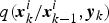 $q({{\bi {x}}_{k}^{i}}/{{\bi {x}}_{k-1}^{i}},{\bi {y}}_{k} )$
. Considering the Gaussian characteristics of the noises in our model, the residual resampling method is used (Beadle and Djuric, Reference Beadle and Djuric1997). As is known, the problem of PF is the sample impoverishment, which means the number of particles may monotonically decrease with time. For the strong nonlinear models we employed, if a large number of particles is used, the filter may spend a long period in computation. However, if a small number of particles is used, sample impoverishment may occur which results in poor estimation performance.
Remark: In the four nonlinear filters, the selection of the process noise variance Q and the measurement noise variance R is very important and difficult. In fact, the sizes of the system model error and the measurement error are the weighted value of the model predictive value and the measurement value, respectively. (1) When R is fixed, larger Q means that the state estimation depends more on the measurement value, and with Q tending to infinity, the state estimation is determined only by the measurement value. On the contrary, smaller Q means that the state estimation depends more on the model predictive value, and with Q being zero, the state estimation is determined only by the model predictive value. (2) When Q is fixed, larger R means that the state estimation depends more on the model predictive value, and with R tending to infinity, the state estimation is determined only by the model predictive value. On the contrary, smaller R means that the state estimation depends more on the measurement value, and with R being zero, the state estimation is determined only by the measurement value.
4. TECHNICAL TOOLS
4.1. Derivation of Theoretical CRLB
From estimation theory, observability of the states is a critical criterion to evaluate the performance of the state estimations. Observability metrics can be easily obtained for linear, time-invariant systems using the observability Gramian, but hard for such strongly nonlinear and time-varying systems as Mars entry. A link between the inverse of the Fisher Information Matrix (FIM) and the observability is established (Jauffret, Reference Jauffret2007). The Cramer-Rao inequality can relate the inverse of FIM to theoretical estimation error covariance lower bound. In order to evaluate the performance of the filters, we resort to CRLB instead of observability analysis. The derivation of CRLB for the discrete-time system is described in (Tichavsky et al., Reference Tichavsky, Muravchik and Nehorai1998). The information matrix obeys the following recursion:
 $${\bi {J}}_{k+1} ={\bi {D}}_k^{22} -{\bi {D}}_k^{21} ({\bi {J}}_k +{\bi {D}}_k^{11})^{-1}{\bi {D}}_k^{12}$$
where
 $$\eqalign{ {\bi {D}}_k^{11} &=E\{{\bi {F}}_k^T {\bi {Q}}^{-1}{\bi {F}}_k \} \cr {\bi {D}}_k^{12} &=-E\{{\bi {F}}_k^T \}{\bi {Q}}^{-1}=[{\bi {D}}_k^{21} ]^T \cr {\bi {D}}_k^{22} &={\bi {Q}}^{-1}+E\{{\bi {H}}_{k+1}^T {\bi {R}}^{-1}{\bi {H}}_{k+1} \} }$$
Note that the Jacobian matrices F and H in the above equations are all calculated at the true states. The derivation of the information matrix above is for the additive Gaussian noise situation, just as in Equations (12) and (16). Then the CRLB which relates the estimate error covariance and the information matrix at time index k can be expressed as below:
 $$\hat{{\bi {P}}}_k (j,j)\ge \hbox{CRLB}\{{\bi {x}}_k (j)\}={\bi {J}}_k^{-1} (j,j),\quad j=1,2,3,4,5,6$$
The initial information matrix
 ${\bi {J}}_{0}$
is the inverse of initial covariance matrix
 $\hat{{\bi {P}}}_{0} $
.
4.2. Consistency Test
A filter is considered to be consistent if its state estimation errors satisfy two conditions: (1) unbiasedness of the state estimations; (2) the actual Mean Square Error (MSE) matches the filter calculated covariance. The consistency evaluation is vital for a filter design because it amounts to the evaluation of a filter's optimality (Bar-Shalom et al., 2001). A commonly used tool for filter consistency is based on the average Normalised Estimation Error Squared (NEES) defined as (Li et al., Reference Li, Zhao and Jilkov2001):
 $$\bar{\varepsilon }_k ={1\over MC\cdot n}\sum_{i=1}^{MC} [\tilde{{\bi {x}}}^i]^T [\hat{{\bi {P}}}^i]^T\tilde{{\bi {x}}}^i$$
where MC is the runs of the Monte Carlo simulation, n is the dimension of states,
 $\tilde{{\bi {x}}}={\bi {x}}-\hat{{\bi {x}}}$
is the estimation errors. Under the assumption that the estimation errors are zero-mean Gaussian, then
 $\bar{\varepsilon}_{k}$
will conform to chi-square distribution with MC·n degrees of freedom. The filter is said to be consistent if
 $$P\{\bar {\varepsilon }_k \in [r_1 ,r_2 ]\}=1-\alpha$$
where [r
1, r
2] is the acceptance interval which can be decided by the following formula at level
 $\alpha =0{\cdot}05$
:
 $$[r_1 ,r_2 ]\approx {1\over 2n\cdot MC}(\pm 1.96+\sqrt {2n\cdot MC-1} )^2$$
5. NUMERICAL SIMULATION AND ANALYSIS
In this section, the detailed simulation results are analysed and discussed. The simulation time is 300 s and the simulation step is 0·5 s. The initial entry conditions listed in Table 1 (Yu et al., Reference Yu, Cui and Zhu2014) and some other parameters of the spacecraft, like the cross-section area s=15·9 m2, the mass m=2804 kg, largely come from the Curiosity spacecraft. Mars rotating angular velocity is
 $\omega_{M}= 7.0882e-5$
rad/s. At equator level, the ground of Mars is
 $V_{M}=\omega_{M}R_{M}=7{\cdot}0882e-5\,\hbox{rad/s}\ast 3397{\cdot}2\,\hbox{km} = 0{\cdot}2408$
km/s, where R
M
is Mars’ radius. In general, Mars entry lasts several minutes, in this paper about 300 s, which means that the target landing site at the equator moves about
 $d=V_{M} t = 0{\cdot}2408\,\hbox{km/s}\ast 300\,\hbox{s} = 72{\cdot}24$
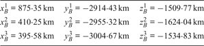
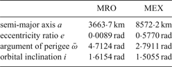
km. For future Mars landing accuracy to be within 100 m of the target (Wolf et al., Reference Wolf, Graves, Powell and Johnson2004), if Mars rotation is not considered, it will not and cannot reach this goal. Mars rotation has to be taken into account. The optimal initial locations of the beacons are listed in Table 2 (Yu et al., Reference Yu, Cui and Zhu2014). The parameters of the two orbiters are listed in Table 3 (Lightsey et al., Reference Lightsey, Mogensen, Burkhart, Ely and Duncan2008). Following are the comparisons of the filters in performance and computation costs.
Initial entry conditions.

Initial locations of the beacons.

Initial entry conditions.

5.1. Estimation Error Analysis
In this subsection, the estimation errors of the four nonlinear filters above are presented. The initial value of the estimation error variance
 ${\bi {P}}_{0}$
, the process noise variance
Q
and the measurement noise variance
R
about the four nonlinear filters are given by
 ${\bi {P}}_{0} = \hbox{diag}\ (1, 1, 1, 1, 1, 1)$
,
 ${\bi {Q}} = \hbox{diag}\ (0{\cdot}1, 0{\cdot}1, 0{\cdot}1, 0{\cdot}1, 0{\cdot}1, 0{\cdot}1)$
,
 ${\bi {R}} = \hbox{diag}\ (100, 100, 100, 100, 100, 1, 1, 1)$
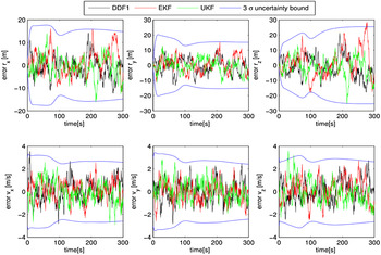
. To make clear comparisons, estimation errors of states and the 3σ standard deviation from EKF, UKF and DDF1 are shown in Figure 2. It can be observed that the estimation performance of EKF, UKF and DDF1 are similar, and the estimation errors are in the same order and are all within the 3σ standard deviation bound.
Comparisons of the estimation errors from EKF, UKF and DDF1 and their 3σ standard deviation.

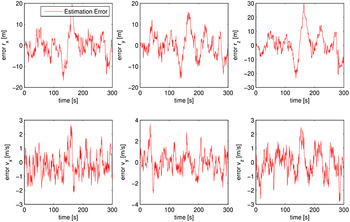
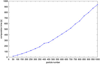
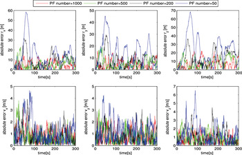
Estimation errors of PF with 1000 particles are shown in Figure 3. This has similar estimation accuracy to the other three filters. However, the computation time for EKF, UKF and DDF1 is 0·4621 s, 1·9310 s, 2·2986 s respectively. While for PF the computation time is 1025.6 s. Mars entry lasts just a few minutes, about 300 s, in which 1025.6 s for the PF is unacceptable and the differences of the computation times for EKF, UKF, DDF1 can be ignored. Theoretically the estimation of PF will converge to the true state as the number of particles tends to infinity (Hu et al., Reference Hu, Schon and Ljung2008), but it is at the price of a large computation time. For the case of Mars entry navigation, the relationship between particle numbers and computation time is shown in Figure 4. The comparisons of the estimation absolute errors from the PF with 1000, 500, 200 and 50 particles are depicted in Figure 5, which indicates that the more particles, the better the estimate performance. All the simulations in this paper are performed by MATLAB in a Windows XP machine with an Intel®Celeron® E1400 CPU processor.
State estimation errors of the PF with 1000 particles.

Particle numbers versus computation time.

Comparisons of the estimation absolute errors from the PF with 1000, 500, 200 and 50 particles.

5.2. Root Mean Square Error (RMSE) Analysis
According to the analysis above, it can be concluded that the PF is inapplicable for Mars entry navigation due to the time limit. In this subsection, further analysis of the lander's position and velocity RMSE is carried out to choose the appropriate navigation filter from the other three. 1000 Monte Carlo (MC) simulation runs are performed. The position and velocity RMSE are:
 $$\eqalign{ \hbox{RMSE}_P &=\sqrt {{1\over MC}\sum_{i=1}^{MC} {[(r_x -\hat{r}_x^i)^2+(r_y -\hat{r}_y^i)^2+(r_z -\hat {r}_z^i )^2]} } }$$
 $$\eqalign{ \hbox{RMSE}_V &=\sqrt {{1\over MC}\sum\limits_{i=1}^{MC} {[(v_x -\hat {v}_x^i )^2+(v_y -\hat {v}_y^i )^2+(v_z -\hat {v}_z^i )^2]} } }$$
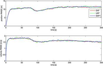
Figure 6 shows the simulation results from which it can be observed that the three filters still have similar performance.
Position and velocity RMSE.

5.3. Error standard deviation versus SR_CRLB
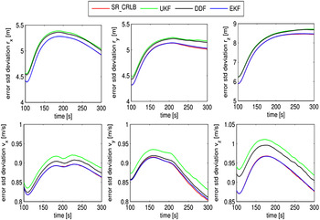
To further compare the performance of the filters, the error standard deviation from EKF, UKF and DDF1 is compared against the SR_CRLB. Figure 7 shows the comparison results from 100 s to 300 s, from which it can be observed that the error standard deviation from EKF is closest to the SR_CRLB and almost coincides with it, which means that EKF is the best in error standard deviation. The green line is on the top of the black line, which means that the DDF is better than the UKF in the case of Mars entry navigation system.
Error standard deviation versus SR_CRLB.

5.4. Consistency Test
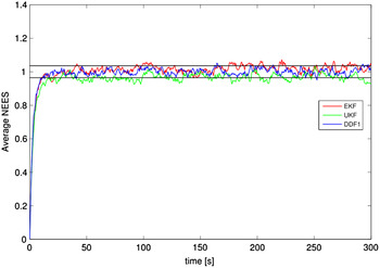
Figure 8 shows the results of the consistency test of EKF, UKF and DDF1 by 1000 Monte Carlo simulations. It can be seen that the average NEES of DDF1 is almost located in the acceptance interval after 50 s, while some parts of the average NEES of EKF and UKF are outside the acceptance interval, which means that the consistency of DDF1 is better than EKF and UKF.
Average NEES.

6. CONCLUSIONS
This paper has studied the problem of Mars entry navigation by using radiometric measurements considering Mars rotation. To make a pinpoint landing, Mars rotation is taken into consideration in both dynamic and measurement models. The performance of four generally used nonlinear filters (EKF, UKF, DDF1, PF) is researched. PF is eliminated first due to computation time limit. EKF, UKF and DDF1 have similar estimation accuracy and computation time. Then the position and velocity RMSE is investigated, which shows that the EKF, UKF and DDF1 still have similar performance. According to the comparison of error standard deviation versus SR_CRLB, it can be seen that the EKF is best, and the DDF1 is better than UKF. Finally, a consistency test was carried out which shows that the DDF1 is better than EKF and UKF, but this could not be considered as the sole criteria to select DDF1 as the navigation filter.
As mentioned in the simulations, although the computation time of the EKF (0·4621 s) is relatively shorter than UKF (1·9310 s) and DDF1 (2·2986 s), the derivation of the Jacobian matrices which are computed in advance is not included in the simulation time. Furthermore, for the dynamic and measurement models of Mars entry with strong nonlinearity, the derivation of the Jacobian matrices is complicated. Therefore, based on the analysis above, the DDF1 is preferred for Mars entry navigation by using radiometric measurements from Mars orbiters and MSBs.
ACKNOWLEDGEMENTS
This work was supported in part by the National Basic Research Program of China (973 Program) under Grant 2012CB720000, in part by the National Natural Science Foundation of China under Grant 61225015, Grant 61105092, Grant 61422102, and Grant 61603365, in part by the Beijing Natural Science Foundation under Grant 4161001, and in part by the Foundation for Innovative Research Groups of the National Natural Science Foundation of China under Grant 61321002.