


1 Introduction
Helical vortices constitute fundamental fluid mechanical objects such as point vortices and vortex rings (Alekseenko, Kuibin & Okulov Reference Alekseenko, Kuibin and Okulov2007). Helical vortices are the oldest mathematical idealization of tip vortices in the wakes behind screws, propellers or wind turbines (Joukowsky Reference Joukowsky1912; Kuibin, Okulov & Pylev Reference Kuibin, Okulov and Pylev2006; Felli, Camussi & Di Felice Reference Felli, Camussi and Di Felice2011; Sherry et al. Reference Sherry, Nemes, Lo Jacono, Blackburn and Sheridan2013; Okulov, Sørensen & Wood Reference Okulov, Sørensen and Wood2015). For a wind turbine, the kinematics and the geometrical form of a system of helical vortices are of special interest, as they may be exploited to determine the optimum rotor efficiency (Okulov & Sørensen Reference Okulov and Sørensen2010). When computing the shape and displacement of a helix, only the binormal component of the velocity is required, as the tangential component does not affect the equilibrium of the helix (e.g. Ricca Reference Ricca1994; Boersma & Wood Reference Boersma and Wood1999; Okulov Reference Okulov2004, and references therein). This was already noted in the pioneering work of Joukowsky (Reference Joukowsky1912), who neglected the tangential component along the helix axis and employed the angular velocity to determine the binormal component. These geometrical particularities of the kinematics of helical vortices will be considered in detail in the following.
Among all helical structures, the infinitely thin helical vortex filament of constant pitch and radius constitutes a fundamental singular object of vortex dynamics. Unfortunately, this mathematical abstraction cannot be exploited directly to determine the helix motion, because the induced velocity becomes infinite on the axis. A real physical helical vortex, on the other hand, has a finite vortex core which can be considered as a superposition of a set of singular helical vortex filaments, resulting in the disappearance of the singularity due to the integration. However, there exist no closed-form solutions taking into account arbitrary vorticity distributions of the vortex core. In spite of this, it is possible to determine the motion of a finite-core helical vortex using the solution for an infinitely thin vortex at some finite distance from the centre of the vortex, and correct it for torsion and curvature effects. Indeed, assuming the particular case of a vortex core with a constant distribution of vorticity, Ricca (Reference Ricca1994) determined a correlation between a finite and an infinite vortex core numerically by combining a filament solution with an extended version of the approximation of the Biot–Savart equations introduced by Moore & Saffman (Reference Moore and Saffman1972). The additional correction term was later analytically derived and proved by Boersma & Wood (Reference Boersma and Wood1999).
Unfortunately, it is complicated to use the above approach directly, because, in contrast to the fundamental cases of a straight line (‘point’) vortex or a vortex ring, the Biot–Savart integral for the flow induced by the helical filament does not have a closed form. Thus, it cannot be represented as a simple pole, such as a point vortex, or expressed as complete elliptic integrals, as for an infinitely thin vortex ring (see e.g. Lamb Reference Lamb1932). There are various ways to determine approximate formulae, including integration of the Biot–Savart law; Kawada–Hardin’s infinite series of the Kapteyn type (Kawada Reference Kawada1936; Hardin Reference Hardin1982; Fukumoto, Okulov & Wood Reference Fukumoto, Okulov and Wood2015), a special form of Boersma & Wood’s  $W$-integral with singularity separation (Boersma & Wood Reference Boersma and Wood1999), or different attempts of exploiting analytical evolutions. The Biot–Savart law can be used in numerical simulations to determine the velocity field in points outside the singular vortex filament. Initially, to simplify the numerical calculations, Kawada (Reference Kawada1936) derived an infinite series as a partial case to the Goldstein (Reference Goldstein1929) solution for the helical vortex wake. Unaware of the pioneering work by Kawada, Hardin (Reference Hardin1982) derived a similar set of equations consisting of the Kapteyn series as an equivalent form to the Biot–Savart law. Next, Ricca (Reference Ricca1994) used this technique for numerical estimations of the induced velocity of a helical filament to compare it with the velocities of a vortex with a finite core. However, this series encountered a problem in achieving accurate results for the flow in the azimuthal direction, owing to errors in approximating the infinite series by a finite array of harmonic terms (see appendix A). Later, Boersma & Wood (Reference Boersma and Wood1999) used the investigation of Ricca (Reference Ricca1994) to derive an integral representation for the remainder,
 $W$, after separating the singularities on the filament in the Kapteyn series to provide a correction for the finite vortex core by integrating it around its cross-section. A general problem with both approaches, however, is that they do not contain closed-form solutions of the equations, because neither the Biot–Savart nor the
 $W$ integrals can be integrated into a closed-form solution, and the Kapteyn series cannot be summed for the infinity harmonics. As a result, it was essentially necessary to develop special analytical approaches. Initially, Kawada (Reference Kawada1936) extracted the two main terms in the Kapteyn series, which, however, were insufficient to arrive at an accurate solution. Independently from his contributions, Okulov (Reference Okulov2004) proposed a more accurate analytical approximation, which included six key terms, resulting in a very fast decaying remainder of the series. In spite of its generality, the result of Okulov (Reference Okulov2004) was only applied as a basic solution to study the stability of helical multiples in a moving coordinate system with additional axial velocity (Okulov & Sørensen Reference Okulov and Sørensen2007). Furthermore, the analytical solution for the motion of a single helix in an immobile (absolute) coordinate system was not considered in the previous works. However, a full analytical solution to the problem will be given in the following.
The paper is organized as follows. In § 2, we give a description of the geometry and kinematics of helical vortices, with the particular aim of describing the self-induced motion of helical vortices. A discussion regarding the correlation between solutions of vortex filaments of infinite thickness and vortex filaments of finite thickness is given in § 3. In § 4, based on the earlier work by Okulov (Reference Okulov2004), we derive a closed-form solution for the binormal velocity, and hence for the induction and motion of a single helical vortex. In § 5 we derive a similar set of equations to describe the full motion of fluid particles along the axis of a helical vortex. Finally, in § 6, we conclude the work.
2 Kinematics of the helical vortices
We start by defining the geometry of a helical vortex of radius  $R$ (figure 1a). The helical pitch,
 $L=2\unicode[STIX]{x03C0}l$, is defined as the axial displacement during one turn of the helix, and the helix angle is determined as
 $\tan \unicode[STIX]{x1D719}=L/2\unicode[STIX]{x03C0}R$, with corresponding helix torsion
 $\unicode[STIX]{x1D70F}=l/R$. Furthermore, the absolute induced velocity
 $u$, is defined either through the binormal velocity,
 $u_{b}$, and the tangential velocity,
 $u_{t}$, or through the axial velocity,
 $u_{z}$, and the azimuthal velocity,
 $u_{\unicode[STIX]{x1D703}}$ (figure 1b). In accordance with remark to equation (7.1.13) of Batchelor (Reference Batchelor1967) the contribution of the normal component
 $u_{n}$ does not lead to displacement of the vortex line and will not be considered here.
(a) Sketch of the induced motion of a material fluid particle, with  $u$ (red arrow) denoting the velocity without azimuthal displacement (
 $\unicode[STIX]{x0394}\unicode[STIX]{x1D703}$), and
 $u_{b}$ (green arrow) denoting the binormal translation of the helical vortex with azimuthal displacement. (b) The helix displacement in cylindrical coordinates (
 $\unicode[STIX]{x1D703}$,
 $z$) on the supporting cylinder of radius
 $R$. The values
 $(u_{Sind})_{z}$ and
 $(u_{Sind})_{\unicode[STIX]{x1D703}}$ denote the translation of the helix in the axial and azimuthal directions.

It should be mentioned that the binormal and the absolute velocity depict the same spatial displacement of the helical vortex structure, as indicated by the blue line and velocity vectors in figure 1(a). For simplicity, we also show the helix as a rectilinear line by a horizontal projection of the cylindrical coordinates ( $\unicode[STIX]{x1D703}$,
 $z$) on a cylindrical surface embedding the helix (figure 1b). From this, it is easily recognized that the helix displacement takes place in the binormal direction and that the tangential velocity does not contribute to the displacement, as it acts along the helix axis. Indeed, the definition of
 $u_{b}$ gives the shortest distance to the displaced helix structure as well as defining the helix angle,
 $\unicode[STIX]{x1D719}$ (see figure 1b). The geometry of the helix results in the following trigonometric relations (figure 1a):
 $$\begin{eqnarray}\displaystyle \tan \unicode[STIX]{x1D719}=\unicode[STIX]{x1D70F};\quad \sin \unicode[STIX]{x1D719}=\unicode[STIX]{x1D70F}/\sqrt{1+\unicode[STIX]{x1D70F}^{2}}\quad \text{and}\quad \cos \unicode[STIX]{x1D719}=1/\sqrt{1+\unicode[STIX]{x1D70F}^{2}}. & & \displaystyle\end{eqnarray}$$
Looking at figure 1(b) it is clear that the velocity of a material fluid particle (red arrow and dot) does not define the helix angle. First, when the tangential velocity is subtracted from it, the pitch angle can be defined as the angle between the remaining vector, which is the binormal component, and the  $z$-direction. The reason is simply that the tangential component acts along the helix axis, hence it will not contribute to the displacement of the helical structure, but only influence the movement of fluid particles along the helix axis. It is important to separate the helix displacement (figure 1b – blue line) and the motion of material fluid particles (the red point on the blue line). From figure 1(b) it is readily seen that all velocity vectors connecting the original (black) vortex line and the displaced (blue) line may determine the displacement of the vortex. However, the binormal component is the only one that uniquely defines the helix displacement through the helix angle
 $\unicode[STIX]{x1D719}$. In contrast to this, the absolute velocity defines the motion of a material fluid particle on the helical vortex, but not the displacement of the helical structure. It should also be mentioned that the value of the tangential velocity depends on the vorticity distribution in the core of the helical vortex, which also makes the definition of the helix position via the absolute velocity
 $u$ more difficult. It may seem obvious that the displacement is dictated uniquely by the binormal velocity component. However, in some recent publications, this has been questioned (see e.g. Fuentes Reference Fuentes2018; Durán Venegas & Le Dizès Reference Durán Venegas and Le Dizès2019), and this is partly the motivation for discussing this issue in the present paper. In much earlier works by prominent fluid mechanical scientists, this issue was not, and should not, be questioned. An example is the paper by Ricca (Reference Ricca1994), where on page 251 it is explicitly noted that ‘the relative displacement in the fluid is given only by
 $u_{b}$, while
 $u_{t}$ yields pure tangential motion along the axis’.
Another important reference is the pioneering work by Joukowsky (Reference Joukowsky1912), which, however, contains a somewhat different approach to determining the motion of a helical vortex.
In figure 2 we have reproduced page 13 from the French translation by Margoulis in 1929 of the paper by Joukowsky (Reference Joukowsky1912). Here the starting point is also to neglect the tangential component, but then he proceeds by determining the angular velocity of the helix. As a basis for the analysis, the Biot–Savart law is employed to approximate the solution of the total velocity  $v$ of all fluids particles, as this ‘velocity coincides with the speed of the vortex ring’,
 $$\begin{eqnarray}\displaystyle v=-\frac{J}{4\unicode[STIX]{x03C0}\unicode[STIX]{x1D70C}}\log \frac{\unicode[STIX]{x1D700}}{2\unicode[STIX]{x1D70C}}, & & \displaystyle\end{eqnarray}$$
where  $J$ is the circulation of the vortex,
 $\unicode[STIX]{x1D700}$ is the core radius and
 $\unicode[STIX]{x1D70C}=R/\text{sin}^{2}\unicode[STIX]{x1D6FC}$, with
 $\unicode[STIX]{x1D6FC}$ being the slope angle of the helix. Further, on page 13, Joukowsky remarks that ‘this result could be expected in advance. Let’s now decompose (figure 8 [of Joukowsky Reference Joukowsky1912]) the velocity
 $\unicode[STIX]{x1D708}$ of the helical vortex filament, whose first component,
 $v\cdot tg\unicode[STIX]{x1D6FC}$ is directed along the tangent to the axis of the vortex, and the other,
 $\unicode[STIX]{x1D708}/\text{cos}\,\unicode[STIX]{x1D6FC}$, follows the tangent to the circumference of the straight section of the cylinder. The first component does not affect the equilibrium of our helical line. But the second component communicates a rotation around the axis of the cylinder, with an angular velocity:
 $\unicode[STIX]{x1D6FA}=v/R\cos \unicode[STIX]{x1D6FC}$’ (end of the translated quote; below, the symbols used in the original paper are replaced by
 $\unicode[STIX]{x1D6E4}\equiv -J$ and
 $\unicode[STIX]{x1D719}\equiv \unicode[STIX]{x03C0}/2-\unicode[STIX]{x1D6FC}$).
The page from Joukowsky (Reference Joukowsky1912) (left) and a reproduction of his figure 8 (right) in which it is shown that the tangential component  $v_{tang}$ does not affect the helix displacement.

As exemplified in Joukowsky’s article, depending on the application, the displacement of a helical vortex requires it to be analysed in different coordinate directions, which do not necessarily coincide with the binormal direction.
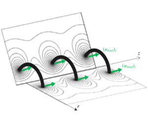
Two main displacements of the vortex-core locations take place in the context of an axial translation of the helix along the axis  $Oz$ or as an azimuthal rotation around the same axis. This is shown in figure 1(b) where the translational velocity is denoted as
 $(u_{Sind})_{z}$ and the azimuthal as
 $(u_{Sind})_{\unicode[STIX]{x1D703}}$. From the figure, it is readily seen that they are not identical to the projections of the binormal velocity
 $u_{b}$. The displacement of the helix in the two orthogonal cross-sections (figure 3) plays an important role in many applications of helical vortices (Alekseenko et al. Reference Alekseenko, Kuibin and Okulov2007). For example, in some applications, the appearance of helical structures in fixed cross-sections are inherent in particle image velocimetry (PIV) measurements of three-dimensional flows (see e.g. Okulov et al. Reference Okulov, Naumov, Mikkelsen, Kabardin and Sørensen2014, Reference Okulov, Kabardin, Mikkelsen, Naumov and Sørensen2019). The motion of a helix in a meridional cross-section,
 $\unicode[STIX]{x1D703}=\text{const}.$ (figure 3a), looks similar to the self-induced motion of vortex rings (Fukumoto & Moffatt Reference Fukumoto and Moffatt2000), and it can be referred to as an axial self-induced motion with the velocity
 $(u_{Sind})_{z}$. The next major displacement of the helix, located in the other orthogonal cross-section
 $z=\text{const}.$ (figure 3b), is recognized as the precession of a helical vortex core (Alekseenko et al. Reference Alekseenko, Kuibin, Okulov and Shtork1999). The frequency
 $\unicode[STIX]{x1D6FA}_{Sind}=(u_{Sind})_{\unicode[STIX]{x1D703}}/R$ of the vortex core precession at
 $z=\text{const}.$ corresponds to the frequency of a concentrated vorticity filament, which e.g. is passing by a fixed anemometer or a PIV laser sheet. As seen in the projections depicted in figure 1(b), the self-induced translation
 $(u_{Sind})_{z}$ and the self-induced rotation
 $(u_{Sind})_{\unicode[STIX]{x1D703}}$ are not identical to the binormal projections
 $(u_{b})_{z}$ and
 $(u_{b})_{\unicode[STIX]{x1D703}}$. Instead, from figure 1(b) one may deduce the following relationships between the various velocity vectors:
 $$\begin{eqnarray}\displaystyle \left.\begin{array}{@{}l@{}}(u_{Sind})_{z}=u_{b}/\text{cos}\unicode[STIX]{x1D719}\quad \text{and}\quad (u_{Sind})_{\unicode[STIX]{x1D703}}=-u_{b}/\text{sin}\unicode[STIX]{x1D719},\text{ while}\\ \qquad (u_{b})_{z}=u_{b}\cos \unicode[STIX]{x1D719}\quad \text{and}\quad (u_{b})_{\unicode[STIX]{x1D703}}=-u_{b}\sin \unicode[STIX]{x1D719}.\end{array}\right\} & & \displaystyle\end{eqnarray}$$
These corrections constitute an inherent part of the interpretation of rotor wakes in earlier works by Okulov & Sørensen (Reference Okulov and Sørensen2010) and in analyses of helix precession (Kuibin & Okulov Reference Kuibin and Okulov1998). It should also be noted that Prandtl (Betz Reference Betz1919), in his treatment of the screw propeller, based the velocity of the screw surface on the projection of the axial self-induced velocity component, i.e.  $u_{b}=(u_{Sind})_{z}\cos \unicode[STIX]{x1D719}$, which then was projected into an axial and an azimuthal component, defining the induced velocities in the wake.
(a) The axial self-induced helix motion in a meridional cross-section,  $\unicode[STIX]{x1D703}=\text{const}.$; (b) the helix precession or self-induced rotation in a fixed cross-section,
 $z=\text{const}$. For both cross-sections the isolines of the streamfunction of the flow are reproduced from the data in § 2.6.2 of Alekseenko et al. (Reference Alekseenko, Kuibin and Okulov2007).

Although the two self-induced components describe the motion of spots of the vorticity concentrations in the two orthogonal cross-sections, they do not coincide with the corresponding projections on the axial and azimuthal directions of either the induced velocity  $u$ of the fluid particles or of the binormal velocity
 $u_{b}$ (figure 1b). From the definition of the helix angle, combining (2.1) and (2.3), we get
 $$\begin{eqnarray}\displaystyle \tan \unicode[STIX]{x1D719}=(u_{Sind})_{z}/(u_{Sind})_{\unicode[STIX]{x1D703}}=(u_{b})_{\unicode[STIX]{x1D703}}/(u_{b})_{z}=l/R\equiv \unicode[STIX]{x1D70F}. & & \displaystyle\end{eqnarray}$$
Other important applications of helix motion include additional global flows. In figure 4 we depict two different situations of superposed flow, with figure 4(a) showing the kinematics and velocity vectors when an axial flow component,  $U_{0}$, is superposed on the helix motion, and figure 4(b) showing a similar picture when the helix is subject to an additional rotation. For a forward propulsion of a propeller or a wake of a wind turbine surrounded by an ambient axial wind field (figure 4a), an additional axial flow velocity superposed on the helix motion needs to be included for a correct definition of the helical pitch in the meridional cross-section (figure 3a). In the investigation of the stability of helical vortex multiples (Okulov Reference Okulov2004), the motion of a moving coordinate system with axial velocity
 $U_{0}=\unicode[STIX]{x1D6E4}N/2\unicode[STIX]{x03C0}l$ was superposed in order to obtain a vanishing induced velocity at the centre, i.e. at
 $r=0$.
The self-induced motions of a helix in two moving systems, ( $O\unicode[STIX]{x1D703}^{\prime }z$) and (
 $O\unicode[STIX]{x1D703}z^{\prime }$), on a supporting cylinder of radius
 $R$. (a) The total helix motion in the axial direction with a supplementary velocity
 $U_{0}$. (b) The total helix rotation with a supplementary angular velocity
 $\unicode[STIX]{x1D6FA}_{0}$.

An additional angular rotation  $\unicode[STIX]{x1D6FA}_{0}$ (figure 4b) can occur in different ways, e.g. by the influence of an additional root vortex (Okulov & Sørensen Reference Okulov and Sørensen2007, Reference Okulov and Sørensen2010), by other vortices in a vortex multiple (Okulov Reference Okulov2004) or by the influence of a boundary (Kuibin & Okulov Reference Kuibin and Okulov1998). It is important to note, as also evidenced on figure 4, that an additional translation automatically implies an additional rotation, and, vice versa, that an additional rotation causes an additional translation.
3 A correlation between solutions for the vortex filament and the vortex of a finite core
The next question we wish to address concerns the possibility of using the induction of a concentrated singular vortex filament to describe the induction from a vortex filament of finite-core size and constant vorticity. For a simple two-dimensional (2-D) vortex it is known that the induction outside the vortex core is the same for a point vortex as for a vortex of finite size, provided that it has a constant vorticity distribution. However, this is not the case for a similar filament of a helical vortex, as the vortex, due to torsion and curvature, induces a non-symmetric velocity field (see references in Kuibin & Okulov Reference Kuibin and Okulov1998). This difference between the induction of a rectilinear (point) vortex and a helical vortex is illustrated in figure 5, which compares the induced azimuthal velocity of a 2-D vortex (figure 5a) and a helical vortex (figure 5b). For the 2-D vortex, it is clearly seen that a point representation of the vortex and a similar vortex of finite-core size generates the same induced velocity field outside the vortex core. In contrast to this, a helical vortex of finite-core size and constant vorticity generates a velocity outside the core that is different from the one generated by a singular vortex filament.
Correlations of azimuthal velocities  $u_{\unicode[STIX]{x1D703}}$ induced by an infinite thin vortex filament (dotted lines) and a vortex with a finite core and a uniform vorticity distribution,
 $\unicode[STIX]{x1D714}_{t}$ (solid lines). (a) Rectilinear vortex and (b) helical filament with constant vorticity (Boersma & Wood Reference Boersma and Wood1999).

A simple way to estimate the velocity at the centre of the vortex is to take the value between two diametrically opposed points on the vortex core, i.e. at  $(r,\unicode[STIX]{x1D703},z)=(R\pm \unicode[STIX]{x1D700},0,0)$, and let the centre velocity be represented by the average of these two values (Ricca Reference Ricca1994; Boersma & Wood Reference Boersma and Wood1999; Okulov Reference Okulov2004, etc.). Although this procedure can immediately be exploited for a 2-D vortex, it requires an additional correction for a helical vortex, since, as discussed above, the induction is non-symmetric.
To determine this correction, consider first the vortex at some point  $O$ with the unit vectors of the natural coordinate system directed along the tangent, and the principal normal and the binormal directions in an orthogonal cross-section of the filament. In this system, the velocity field induced by a curved vortex filament may, at a small distance
 $\unicode[STIX]{x1D70E}$ from the filament, be asymptotically represented as the sum of a pole, a logarithmic singularity and a regular (non-singular) term (Batchelor Reference Batchelor1967). The first of these terms describes the circulatory motion around the vortex axis and does not cause any displacement. The next two terms describe the motion of the vortex filament in the binormal direction. In dimensionless form, scaled with
 $\unicode[STIX]{x1D6E4}\unicode[STIX]{x1D705}/4\unicode[STIX]{x03C0}$, the binormal velocity is given as,
 $$\begin{eqnarray}\displaystyle {\hat{w}}_{b}^{(Asympt)}=-\frac{2\cos \unicode[STIX]{x1D703}}{\unicode[STIX]{x1D705}\unicode[STIX]{x1D70C}}+\ln \frac{1}{\unicode[STIX]{x1D705}\unicode[STIX]{x1D70C}}+C^{(Asympt)}, & & \displaystyle\end{eqnarray}$$
where  $\unicode[STIX]{x1D70C}$,
 $\unicode[STIX]{x1D703}$ are the polar coordinates of the natural system and
 $\unicode[STIX]{x1D705}$ is the vortex curvature.
It is known (Ricca Reference Ricca1994; Kuibin & Okulov Reference Kuibin and Okulov1998) that the dimensionless self-induced velocity of a helical vortex with a finite-core size of  $\unicode[STIX]{x1D700}$ after integration of (3.1) is described by the formula,
 $$\begin{eqnarray}\displaystyle {\hat{w}}_{b}^{(Sind)}=\ln \frac{1}{\unicode[STIX]{x1D705}\unicode[STIX]{x1D700}}+C^{(Sind)}, & & \displaystyle\end{eqnarray}$$
where  $\unicode[STIX]{x1D700}$ is the radius of the vortex core. This can be considered as an analogue to (3.1) without the pole, which vanishes from the integral because of the symmetry of the pole contribution. The disappearance of the pole and the logarithmic term provides a basis for utilizing the velocity induced by a filament at a distance
 $\unicode[STIX]{x1D70C}=\unicode[STIX]{x1D700}$ to represent the flow field induced by a vortex of finite-core size,
 $\unicode[STIX]{x1D700}$. However, it remains to estimate the last term of the two equations to complete the interrelation between the quantities. In (3.1) the quantity
 $C^{(Asympt)}$ only depends on the geometry of the vortex filament, whereas the value of
 $C^{(Sind)}$ in (3.2), together with the same geometric vortex parameters, also depends on the vorticity distribution inside the vortex core (Batchelor Reference Batchelor1967; Tung & Ting Reference Tung and Ting1967; Ricca Reference Ricca1994; Kuibin & Okulov Reference Kuibin and Okulov1998; Boersma & Wood Reference Boersma and Wood1999; Okulov Reference Okulov2004 etc.). This difference between the ‘
 $C$’ terms can take different values, depending on the form of the core and the vorticity distribution of the vortex. As an example, the value for a vortex ring with uniform vorticity of the core was determined to be
 $3/4$ by Tung & Ting (Reference Tung and Ting1967). For a helical vortex, the difference is
 $1/4$, as was analytically deduced by Boersma & Wood (Reference Boersma and Wood1999), who showed that
 $$\begin{eqnarray}\displaystyle C^{(Sind)}=C^{(Asympt)}+{\textstyle \frac{1}{4}}. & & \displaystyle\end{eqnarray}$$
Although (3.3) represents a simple way of establishing a finite-core vortex solution from the solution of a similar vortex of zero thickness, the correction seems not to be generally known. A recent example of this is the paper by Fuentes (Reference Fuentes2018), where the integral representation of Boersma & Wood (Reference Boersma and Wood1999) for the Kawada–Hardin solution of the helical filament was used directly to compute the motion of the helical vortex without using (3.3) to correct it for the finite-core vortex.
4 The motion of a single helical vortex
As a basis for determining the motion of a single helical vortex, we employ the Kapteyn series employed in Kawada–Hardin’s solution (Hardin Reference Hardin1982). This series was originally written as
 $$\begin{eqnarray}\displaystyle H^{I,J}(a,b,\unicode[STIX]{x1D712})=\mathop{\sum }_{m=1}^{\infty }m\text{I}_{m}^{\langle I\rangle }(ma)\text{K}_{m}^{\langle J\rangle }(mb)\cdot \text{e}^{\text{i}m\unicode[STIX]{x1D712}}, & & \displaystyle\end{eqnarray}$$
where  $\text{I}_{m}^{\langle 0\rangle }(ma)$ and
 $\text{K}_{m}^{\langle 0\rangle }(mb)$ are the modified Bessel functions, and
 $\text{I}_{m}^{\langle 1\rangle }(ma)$ and
 $\text{K}_{m}^{\langle 1\rangle }(mb)$ are their respective derivatives; the parameter
 $a$ denotes the dimensionless radial distance to the point considered, and
 $b$ denotes the dimensionless radius of the vortex, both made dimensionless by the helical pitch
 $l$ or something similar via helix torsion
 $\unicode[STIX]{x1D70F}=l/R$. Okulov (Reference Okulov2004) derived an accurate analytical approximation of the Kapteyn series (4.1), which included six key terms with remainder terms that were sufficiently small to be neglected. In spite of its potential generality, this result was applied only to investigate the stability of helical multiples in a moving coordinate system with an additional axial velocity (Okulov Reference Okulov2004; Okulov & Sørensen Reference Okulov and Sørensen2007). To generalize and complete the equations of motion for a single helical vortex located in a non-moving frame of reference, we here revisit the work by Okulov (Reference Okulov2004) and derive the missing equations.
In accordance with the procedure described by Okulov (Reference Okulov2004), an analytical form of the infinite series (4.1) (using appendix A), can be determined as follows:
(i) for the point
 $R-\unicode[STIX]{x1D70E}R<R$ inside of the helix: (4.2)$$\begin{eqnarray}\displaystyle H^{0,1}\left(\frac{1-\unicode[STIX]{x1D70E}}{\unicode[STIX]{x1D70F}},\frac{1}{\unicode[STIX]{x1D70F}},0\right) & = & \displaystyle \frac{1}{4}\frac{\unicode[STIX]{x1D70F}^{2}}{(1+\unicode[STIX]{x1D70F}^{2})^{1/2}}\left(-\frac{2}{\unicode[STIX]{x1D70E}}\right)\nonumber\\ \displaystyle & & \displaystyle +\,\frac{1}{4}\frac{\unicode[STIX]{x1D70F}^{2}}{(1+\unicode[STIX]{x1D70F}^{2})^{3/2}}\left(\ln (\unicode[STIX]{x1D70E})+\ln \left(\frac{\sqrt{1+\unicode[STIX]{x1D70F}^{2}}}{2}\right)+\unicode[STIX]{x1D70F}^{2}-1\right)\nonumber\\ \displaystyle & & \displaystyle +\,\frac{1}{4}\frac{\unicode[STIX]{x1D70F}^{2}}{(1+\unicode[STIX]{x1D70F}^{2})^{9/2}}\!\left[\frac{27}{8}+2\unicode[STIX]{x1D70F}^{4}+\frac{1}{\unicode[STIX]{x1D70F}^{2}}-\left(\!\unicode[STIX]{x1D70F}^{4}-3\unicode[STIX]{x1D70F}^{2}+\frac{3}{8}\right)\unicode[STIX]{x1D70D}(3)\right]\nonumber\\ \displaystyle & & \displaystyle +\,I_{1}\left(\frac{1}{\unicode[STIX]{x1D70F}}\right)K_{1}^{\prime }\left(\frac{1}{\unicode[STIX]{x1D70F}}\right)+\frac{3\unicode[STIX]{x1D70F}}{4}+o(1),\end{eqnarray}$$
(ii) for the point
$R+\unicode[STIX]{x1D70E}R>R$ outside of the helix (4.3)where$$\begin{eqnarray}\displaystyle H^{1,0}\left(\frac{1}{\unicode[STIX]{x1D70F}},\frac{1+\unicode[STIX]{x1D70E}}{\unicode[STIX]{x1D70F}},0\right) & = & \displaystyle \frac{1}{4}\frac{\unicode[STIX]{x1D70F}^{2}}{(1+\unicode[STIX]{x1D70F}^{2})^{1/2}}\left(\frac{2}{\unicode[STIX]{x1D70E}}\right)\nonumber\\ \displaystyle & & \displaystyle +\,\frac{1}{4}\frac{\unicode[STIX]{x1D70F}^{2}}{(1+\unicode[STIX]{x1D70F}^{2})^{3/2}}\left(\ln (\unicode[STIX]{x1D70E})+\ln \left(\frac{\sqrt{1+\unicode[STIX]{x1D70F}^{2}}}{2}\right)+\unicode[STIX]{x1D70F}^{2}-1\right)\nonumber\\ \displaystyle & & \displaystyle +\,\frac{1}{4}\frac{\unicode[STIX]{x1D70F}^{2}}{(1+\unicode[STIX]{x1D70F}^{2})^{9/2}}\!\left[\frac{27}{8}+2\unicode[STIX]{x1D70F}^{4}+\frac{1}{\unicode[STIX]{x1D70F}^{2}}-\left(\!\unicode[STIX]{x1D70F}^{4}-3\unicode[STIX]{x1D70F}^{2}+\frac{3}{8}\right)\unicode[STIX]{x1D70D}(3)\right]\nonumber\\ \displaystyle & & \displaystyle +\,I_{1}\left(\frac{1}{\unicode[STIX]{x1D70F}}\right)K_{1}^{\prime }\left(\frac{1}{\unicode[STIX]{x1D70F}}\right)+\frac{\unicode[STIX]{x1D70F}}{4}+o(1),\end{eqnarray}$$$\unicode[STIX]{x1D70E}=\unicode[STIX]{x1D700}/R$, $\unicode[STIX]{x1D701}(\cdot )$ is the Riemann zeta function, and $o(1)$ is the remainder of the approximation.


As demonstrated by the excellent agreement between (4.2) and (4.3) and the Kapetyn series in figure 6(a), the remainder is clearly seen to be negligibly small. In cylindrical coordinates ( $r$,
 $\unicode[STIX]{x1D703}$,
 $z$), according to the Kawada–Hardin solution, the axial and azimuthal velocity components induced by the helical vortex outside of the core are given as
 $$\begin{eqnarray}\displaystyle u_{\unicode[STIX]{x1D703}}(r,R,\unicode[STIX]{x1D712})=\frac{\unicode[STIX]{x1D6E4}}{2\unicode[STIX]{x03C0}r}\left\{\begin{array}{@{}l@{}}0\\ 1\end{array}\right\}+\frac{\unicode[STIX]{x1D6E4}a}{\unicode[STIX]{x03C0}rl}\left\{\begin{array}{@{}l@{}}H^{0,1}(r/l,R/l,\unicode[STIX]{x1D712})\\ H^{1,0}(R/l,r/l,\unicode[STIX]{x1D712})\end{array}\right\}\!,\quad u_{z}(r,R,\!\unicode[STIX]{x1D712})=\frac{\unicode[STIX]{x1D6E4}}{2\unicode[STIX]{x03C0}l}-\frac{r}{l}u_{\unicode[STIX]{x1D703}}(r,R,\!\unicode[STIX]{x1D712}), & & \displaystyle \nonumber\\ \displaystyle & & \displaystyle\end{eqnarray}$$
where  $\unicode[STIX]{x1D712}=\unicode[STIX]{x1D703}-z/l$, and the upper expression in braces corresponds to the case
 $r<R$, and the lower one to
 $r>R$. Figure 6(b) also shows an excellent agreement between the simulations of
 $u_{\unicode[STIX]{x1D703}}$ using the Kapteyn series (4.1) and the analytical forms of (4.2) and (4.3) with
 $\unicode[STIX]{x1D6E4}=4\unicode[STIX]{x03C0}$,
 $\unicode[STIX]{x1D712}=0$ and
 $\unicode[STIX]{x1D70E}=0.1$.
(a) Correlations of the Kapteyn series (3.2) with 70 harmonics (dots) and the analytical equivalent (3.3)–(4.1) (solid lines). (b) Azimuthal velocities  $u_{\unicode[STIX]{x1D703}}$ computed symmetrically around the helix axis at external positions,
 $r/R=1+\unicode[STIX]{x1D70E}$, and at internal positions,
 $r/R=1-\unicode[STIX]{x1D70E}$, using (4.2) combined with (3.2) and (3.3)–(4.1). (All simulations in the plots hereinafter were undertaken with
 $\unicode[STIX]{x1D6E4}=4\unicode[STIX]{x03C0}$ and
 $\unicode[STIX]{x1D70E}=0.1$.)

The new form of the solution (4.4) by (4.2) and (4.3) with the pole and logarithmic singularities is fully in line with the asymptotic development (3.1) for the velocity field induced by any curved infinite thin vortex filament (Batchelor Reference Batchelor1967). The development (4.2) and (4.3) predicts an infinite speed on the helical filament, and the induction velocity (4.4) cannot be directly applied to estimate the translation of a helical vortex with finite core or the motion of fluid particles along the helical axis. For this purpose, the non-singular term in (3.2) needs to be determined. A way to do this was proposed by Ricca (Reference Ricca1994), who used the half-sum of the filament velocities (4.4) at two points diametrically placed at  $\unicode[STIX]{x1D70E}=\pm \unicode[STIX]{x1D700}/R$ from the filament. As discussed in § 3, the asymptotic singular term needs to be further corrected by a constant in order to represent the value at the vortex centre. By subtracting the pole
 $1/\unicode[STIX]{x1D70E}$ and the logarithm pole
 $\ln (1/\unicode[STIX]{x1D70E})$ from the original Kapteyn series (4.1), Ricca (Reference Ricca1994) predicted numerically that the correction in (3.3) should be approximately
 $1/4$. This was later confirmed analytically by Boersma & Wood (Reference Boersma and Wood1999), who separated both singularities by an analytical reorganization of the equations, resulting in the representation of the remainder by an integral,
 $$\begin{eqnarray}\displaystyle W(\unicode[STIX]{x1D70F})=\int _{0}^{\infty }\left\{\frac{\sin ^{2}t}{[\unicode[STIX]{x1D70F}^{2}t^{2}+\sin ^{2}t]^{3/2}}-\frac{1}{[\unicode[STIX]{x1D70F}^{2}+1]^{3/2}}\frac{T(1/2-t)}{t}\right\}\text{d}t, & & \displaystyle\end{eqnarray}$$
where  $T(\cdot )$ denotes the unit step function. The integral remainder (4.5) describes the main effect of vortex torsion. The expression is regular and permits us to prove analytically the
 $1/4$-term in (3.3). However, it cannot be integrated into a closed form, just as the Biot–Savart law for the helical vortex filament, and instead it was numerically determined to an accuracy of six significant figures and tabulated for 21 values of the pitch
 $\unicode[STIX]{x1D70F}$. Based on this analysis, Boersma & Wood (Reference Boersma and Wood1999) for the first time derived a realistic formula for the binormal velocity
 $u_{b_{B\& W}}$ of a helical vortex with finite core,
 $$\begin{eqnarray}\displaystyle & & \displaystyle \frac{4\unicode[STIX]{x03C0}R}{\unicode[STIX]{x1D6E4}}u_{b_{B\& W}}=\frac{1}{1+\unicode[STIX]{x1D70F}^{2}}\nonumber\\ \displaystyle & & \displaystyle \quad \times \left[\ln \left(\frac{2}{\unicode[STIX]{x1D70E}}\right)-\frac{1}{4}+2\unicode[STIX]{x1D70F}^{2}-2\unicode[STIX]{x1D70F}\sqrt{1+\unicode[STIX]{x1D70F}^{2}}-\ln \sqrt{1+\unicode[STIX]{x1D70F}^{2}}+(1+\unicode[STIX]{x1D70F}^{2})^{3/2}W(\unicode[STIX]{x1D70F})\right].\qquad\end{eqnarray}$$
As an alternative to the semi-analytical equation (4.6), the analytical representation of the series, equations (4.2) and (4.3), may be exploited in a similar way as in Ricca (Reference Ricca1994). After some manipulations, we arrive at the following closed analytical form for the velocity of the binormal translation of the axis of a helical vortex of finite-core radius,  $\unicode[STIX]{x1D70E}=\unicode[STIX]{x1D700}/R$,
 $$\begin{eqnarray}\displaystyle \frac{4\unicode[STIX]{x03C0}R}{\unicode[STIX]{x1D6E4}}u_{b} & = & \displaystyle \frac{1}{1+\unicode[STIX]{x1D70F}^{2}}\left[\ln \frac{1}{\unicode[STIX]{x1D70E}}-\frac{1}{4}-\frac{3}{2}\ln \frac{\unicode[STIX]{x1D70F}}{1+\unicode[STIX]{x1D70F}^{2}}+2+\unicode[STIX]{x1D70F}^{2}-\frac{\sqrt{1+\unicode[STIX]{x1D70F}^{2}}(1+3\unicode[STIX]{x1D70F}^{2})}{\unicode[STIX]{x1D70F}}\right]\nonumber\\ \displaystyle & & \displaystyle +\,\frac{\unicode[STIX]{x1D70F}^{2}}{(1+\unicode[STIX]{x1D70F}^{2})^{4}}\left[\left(\unicode[STIX]{x1D70F}^{4}-3\unicode[STIX]{x1D70F}^{2}+\frac{3}{8}\right)\unicode[STIX]{x1D70D}(3)-\frac{27}{8}+2\unicode[STIX]{x1D70F}^{4}+\frac{1}{\unicode[STIX]{x1D70F}^{2}}\right]\nonumber\\ \displaystyle & & \displaystyle +\,4\frac{\sqrt{1+\unicode[STIX]{x1D70F}^{2}}}{\unicode[STIX]{x1D70F}^{2}}I_{1}\left(\frac{1}{\unicode[STIX]{x1D70F}}\right)K_{1}^{\prime }\left(\frac{1}{\unicode[STIX]{x1D70F}}\right)+o(1).\end{eqnarray}$$
In figure 7(a), the binormal velocity is computed as a function of torsion using the new analytical expression (4.7) (solid line) and compared to the solution of Boersma & Wood (Reference Boersma and Wood1999), using the  $W$-integral formulation (4.6), and to that of Ricca (Reference Ricca1994), using a Kapteyn series with 70 terms. As seen, there is an excellent agreement between the three methods. In figure 7(b) the angular self-induced velocity is compared to direct Navier–Stokes simulations of Selçuk, Delbende & Rossi (Reference Selçuk, Delbende and Rossi2017). The comparison is seen to be excellent, verifying both the validity of (4.7) and the explanations and equations derived in § 2 (equations (2.1)–(2.4) and figures 1b and 3b).
(a) Correlations of the non-dimensional binormal velocity of a helical vortex calculated by different methods. Points indicate values of Ricca’s approach via Kapteyn series with 70 harmonics (3.2); squares are  $u_{b_{B\& W}}$ of Boersma & Wood’s formula (4.4a,b); solid line is the current analytical expression (4.5). (b) Comparison of angular velocity
 $\unicode[STIX]{x1D6FA}_{Sind}=(-u_{b}/\text{sin}\unicode[STIX]{x1D719})/R$ in a fixed cross-section (figures 1b and 3b). Solid line: calculation using (4.5); square dots: angular velocity obtained from Navier–Stokes simulations of helix development (Selçuk et al. Reference Selçuk, Delbende and Rossi2017).

Thus, for the first time, a closed-form solution, equation (4.7), has been established to describe the displacement of a helical vortex with a uniform vorticity distribution of the vortex core.
5 The motion of fluid particles along the axis of a helical vortex
In some cases, it is preferable to consider the absolute motion of material fluid elements on the helical axis. However, it is important to emphasize that this motion does not correspond to the motion of the helical structure, and one has to be cautious when trying to derive the displacement of a helical structure from the absolute velocity of the material fluid elements located on the helix axis (figure 8).
Different nature of the absolute motion of the fluid particles along the helical axis and the motion of the helical vortex of the rotor wake in the meridional cross-section is illustrated by a recent example with dye visualization of Quaranta, Bolnot & Leweke (Reference Quaranta, Bolnot and Leweke2015).

As an example, in figures 1(a) and 3(a) it is shown that an axial translation of a helix in a fixed axial cross-section is associated with an additional rotation of the helix. This effect cannot be included when considering the helix motion to be determined purely by the motion of the material fluid particles along the helix axis. The incompatibility between the movement of fluid particles and of the helix is illustrated in the visualization of Quaranta et al. (Reference Quaranta, Bolnot and Leweke2015) (figure 8), where fluid particles are seen to move along the helix axis towards the rotor blade at the same time as the helical wake moves downstream from the rotor.
On the other hand, the absolute velocity  $u$ may play a key role when analysing disturbances and instabilities (Widnall Reference Widnall1972; Hattori & Fukumoto Reference Hattori and Fukumoto2009), or the expansion of the original helical vortex. In these cases, it is necessary to know the absolute velocity components (4.4). As done previously, the analytical form of the Kapteyn series, equations (4.2) and (4.3), combined with (4.4), will be used to derive the analytical expressions for the velocities. Furthermore, we will apply the same approach as the one used to derive the binormal components in the previous section. As before, we utilize the assumption that the velocity on the helix axis can be represented by the sum of the induced velocities at opposite points of the filament, corrected by the non-singularity term (
 $1/4$). However, the correction using the
 $1/4$-term should only be applied for the binormal component, as a uniform distribution of vorticity does not affect the tangential motion of the fluid particles along the helical axis. Hence, the
 $1/4$-term only contributes indirectly to the expression for
 $u_{\unicode[STIX]{x1D703}}$ and
 $u_{z}$ through the corrected binormal velocity, which subsequently is projected onto the azimuthal and axial directions by multiplication of
 $-\text{sin}\,\unicode[STIX]{x1D719}=-\unicode[STIX]{x1D70F}/\sqrt{1+\unicode[STIX]{x1D70F}^{2}}$ and
 $\cos \unicode[STIX]{x1D719}=1/\sqrt{1+\unicode[STIX]{x1D70F}^{2}}$, respectively. Finally, the analytical formulae for the azimuthal and axial components take the form
 $$\begin{eqnarray}\displaystyle \frac{4\unicode[STIX]{x03C0}R}{\unicode[STIX]{x1D6E4}}u_{\unicode[STIX]{x1D703}} & = & \displaystyle \frac{-\unicode[STIX]{x1D70F}}{(\sqrt{1+\unicode[STIX]{x1D70F}^{2}})^{3}}\left[\ln \frac{1}{\unicode[STIX]{x1D70E}}-\frac{1}{4}+\ln \frac{\unicode[STIX]{x1D70F}}{\sqrt{1+\unicode[STIX]{x1D70F}^{2}}}+2-\frac{2}{\unicode[STIX]{x1D70F}}(\sqrt{1+\unicode[STIX]{x1D70F}^{2}})^{3}\right]\nonumber\\ \displaystyle & & \displaystyle +\,\frac{4}{\unicode[STIX]{x1D70F}}I_{1}\left(\frac{1}{\unicode[STIX]{x1D70F}}\right)K_{1}^{\prime }\left(\frac{1}{\unicode[STIX]{x1D70F}}\right)+1-\frac{\unicode[STIX]{x1D70F}}{\sqrt{1+\unicode[STIX]{x1D70F}^{2}}}\nonumber\\ \displaystyle & & \displaystyle -\,\frac{\unicode[STIX]{x1D70F}^{3}}{(\sqrt{1+\unicode[STIX]{x1D70F}^{2}})^{9}}\left[\left(\unicode[STIX]{x1D70F}^{4}-3\unicode[STIX]{x1D70F}^{2}+\frac{3}{8}\right)\unicode[STIX]{x1D70D}(3)-\frac{27}{8}+2\unicode[STIX]{x1D70F}^{4}+\frac{1}{\unicode[STIX]{x1D70F}^{2}}\right]+o(1),\end{eqnarray}$$
 $$\begin{eqnarray}\displaystyle \frac{4\unicode[STIX]{x03C0}R}{\unicode[STIX]{x1D6E4}}u_{z} & = & \displaystyle \frac{1}{(\sqrt{1+\unicode[STIX]{x1D70F}^{2}})^{3}}\left[\ln \frac{1}{\unicode[STIX]{x1D70E}}-\frac{1}{4}+\ln \frac{\unicode[STIX]{x1D70F}}{\sqrt{1+\unicode[STIX]{x1D70F}^{2}}}-2\unicode[STIX]{x1D70F}^{2}\right]\nonumber\\ \displaystyle & & \displaystyle -\,\frac{1}{\unicode[STIX]{x1D70F}}\left(\frac{4}{\unicode[STIX]{x1D70F}}I_{1}\left(\frac{1}{\unicode[STIX]{x1D70F}}\right)K_{1}^{\prime }\left(\frac{1}{\unicode[STIX]{x1D70F}}\right)+1-\frac{\unicode[STIX]{x1D70F}}{\sqrt{1+\unicode[STIX]{x1D70F}^{2}}}\right.\nonumber\\ \displaystyle & & \displaystyle -\left.\frac{\unicode[STIX]{x1D70F}^{3}}{(\sqrt{1+\unicode[STIX]{x1D70F}^{2}})^{9}}\left[\left(\unicode[STIX]{x1D70F}^{4}-3\unicode[STIX]{x1D70F}^{2}+\frac{3}{8}\right)\unicode[STIX]{x1D70D}(3)-\frac{27}{8}+2\unicode[STIX]{x1D70F}^{4}+\frac{1}{\unicode[STIX]{x1D70F}^{2}}\right]\right)+o(1).\quad\end{eqnarray}$$
To verify these simple analytical expressions, the resulting velocities are compared to similar results obtained using a Kapteyn series with 70 harmonics. The outcome of this is depicted in figure 9, which compares the absolute velocities at the helix axis as a function of torsion. It may be argued that replacing the standard Kapteyn solution by a closed-form analytical solution is of minor importance. However, it may become important when investigating the stability properties of a helix in the vicinity of a stable state or when using particle tracking of a large number of fluid particles.
Finally, to demonstrate that the tangential velocity of the helix does not depend on the  $1/4$-term of the correction in (3.3), we substitute the expression (5.1) and (5.2) for
 $u_{\unicode[STIX]{x1D703}}$ and
 $u_{z}$ into the expression for the tangential velocity,
 $u_{t}=(u_{\unicode[STIX]{x1D703}}+\unicode[STIX]{x1D70F}u_{z})/\sqrt{1+\unicode[STIX]{x1D70F}^{2}}$, derived by Ricca (Reference Ricca1994). After some trivial, albeit tedious, transformations, we arrive at the dimensionless formula
 $$\begin{eqnarray}\displaystyle u_{t}=2\frac{\sqrt{1+\unicode[STIX]{x1D70F}^{2}}-\unicode[STIX]{x1D70F}}{1+\unicode[STIX]{x1D70F}^{2}}, & & \displaystyle\end{eqnarray}$$
which clearly is seen not to contain the  $1/4$-term.


Thus, the analytical solutions, equations (5.1) and (5.2), for the motion of fluid particles along the helical axis differ from the binormal displacement of the helical vortex, equation (4.7), and the tangential velocity (5.3) does not affect this motion. Furthermore,  $u_{t}$ does not contribute to the correction, equation (3.3), when considering a uniform vorticity distribution in the vortex core.
6 Conclusions
In this paper, we have derived a set of analytical equations for the motion of helical vortices. We have demonstrated that the kinematics of a helical vortex moving due to self-induction is fundamentally different from the motion of the material fluid elements forming the vortex. In particular, we show that the motion of the vortex is governed solely by the binormal component of the induced velocity. Furthermore, we have derived a set of closed-form equations describing both the binormal component of the velocity, constituting the movement of the helical vortex structure, and the velocity components describing the motion of a material fluid particle located at the centre of the vortex. The analysis was restricted to vortices with a constant vorticity distribution in the vortex core. Solutions for other typical distributions of vorticity of the vortex core will be the subject for future investigations.
Appendix A. A correct evolution of the Kapteyn series
In this appendix we assess the accuracy of the proposed analytical formulae and demonstrate the advantage of employing an analytical form of the equations.
The Kapteyn series (4.1) consists of the harmonic terms along the azimuthal direction,
 $$\begin{eqnarray}\displaystyle & \displaystyle hi_{m}(x,\unicode[STIX]{x1D712})=m\text{I}_{m}^{\langle 0\rangle }(m\cdot a)\text{K}_{m}^{\langle 1\rangle }(m\cdot ax)\cdot \text{e}^{\text{i}m\unicode[STIX]{x1D712}},\quad \text{when }x\leqslant 1; & \displaystyle\end{eqnarray}$$
 $$\begin{eqnarray}\displaystyle & \displaystyle he_{m}(x,\unicode[STIX]{x1D712})=m\text{I}_{m}^{\langle 1\rangle }(m\cdot a)\text{K}_{m}^{\langle 0\rangle }(m\cdot ax)\cdot \text{e}^{\text{i}m\unicode[STIX]{x1D712}},\quad \text{when }x>1. & \displaystyle\end{eqnarray}$$
 $m$-values, with
 $a=R/l=1/\unicode[STIX]{x1D70F}$ and
 $x=r/R$, in agreement with (4.2)–(4.4).
Examples of the harmonic terms  $hi_{m}$ and
 $he_{m}$ of the Kapteyn series (A 1a,b) along the radial (
 $\unicode[STIX]{x1D712}=0$) and azimuthal (
 $x=1$) directions for
 $a=1$.

Examples of the sums  $Hi_{M}$ and
 $He_{M}$ for a direct simulation (A 2a,b) of the Kapteyn series along the radial (
 $\unicode[STIX]{x1D712}=0$) and azimuthal (
 $x=1$) directions for
 $a=1$.

Unfortunately, when carrying out simulations, only finite sums of the harmonics of (A 1) can be utilized,
 $$\begin{eqnarray}\displaystyle Hi_{M}(x,\unicode[STIX]{x1D712})=\mathop{\sum }_{m=1}^{M}hi_{m}(x,\unicode[STIX]{x1D712})\quad \text{or}\quad He_{M}(x,\unicode[STIX]{x1D712})=\mathop{\sum }_{m=1}^{M}he_{m}(x,\unicode[STIX]{x1D712}). & & \displaystyle\end{eqnarray}$$
Figure 11 demonstrates that finite sums of (A 2) cannot describe the singularities of the solution (4.4) at  $x=1$ and
 $\unicode[STIX]{x1D712}=0$. Here, the sums (A 2) predict finite values at
 $\unicode[STIX]{x1D712}=0$ and
 $x=1$, which depend on the number of modes
 $M$. In fact, in order to reach the correct result that the Kapteyn series tends to infinity at
 $x=1$ and
 $\unicode[STIX]{x1D712}=0$, it is required that
 $M\rightarrow \infty$, which makes it inconvenient to use directly the series. Furthermore, in all regular points,
 $\unicode[STIX]{x1D712}\neq 0$, the curves parasitically oscillate, because a regular solution in these points only can be achieved by summing an infinite number of terms from the positive and negative harmonics of the Kapteyn series.
The problem with the simulation of the Kapteyn series is known as ‘problem 97-18’ (Boersma & Yakubovich Reference Boersma and Yakubovich1998). Boersma & Wood (Reference Boersma and Wood1999) separated a simple pole of  $1/x$ type to provide a correction for the velocity field around the helical filament. After the separation they employed an integral form (4.5) for the remainder, which was derived in the paper by Boersma & Yakubovich (Reference Boersma and Yakubovich1998). The integral remainder
 $W$ describes the main effect of vortex torsion and is regular, but cannot be integrated in a closed form, just as the Biot–Savart law for the helical vortex filament. Nevertheless, it was numerically calculated with high accuracy to six significant figures and tabulated in table 1 of Boersma & Wood (Reference Boersma and Wood1999) for 21 values of the pitch
 $\unicode[STIX]{x1D70F}$. We have used these values as a basis to test our analytical representations (see e.g. the squares in figure 7a).
A special analytical approach in which the main singular terms were directly extracted in the Kapteyn series was developed by Kawada (Reference Kawada1936) for the two first terms and independently by Okulov (Reference Okulov2004), who proposed a general algorithm to separate key terms from the series,
 $$\begin{eqnarray}\displaystyle & \displaystyle H^{0,1}(ax,a,\unicode[STIX]{x1D712})=S_{k}^{+}(x,\unicode[STIX]{x1D712})+\mathop{\sum }_{m=1}^{\infty }ri_{m}^{\langle k\rangle }(x)\cdot \text{e}^{\text{i}m\unicode[STIX]{x1D712}}, & \displaystyle\end{eqnarray}$$
 $$\begin{eqnarray}\displaystyle & \displaystyle H^{1,0}(a,ax,\unicode[STIX]{x1D712})=S_{k}^{-}(x,\unicode[STIX]{x1D712})+\mathop{\sum }_{m=1}^{\infty }re_{m}^{\langle k\rangle }(x)\cdot \text{e}^{\text{i}m\unicode[STIX]{x1D712}}, & \displaystyle\end{eqnarray}$$
 $S_{k}$ refers to the main
 $k$ terms representing the series and the sums represent the remainder terms of the series. In accordance with the procedure described by Okulov (Reference Okulov2004) the main analytical form of the Kapteyn series can be determined by a development of (4.1) via
 $k$ terms consisting of two singularities and (
 $k-2$) polylogarithms. Figure 5 in Okulov (Reference Okulov2004) shows a very good correlation of
 $S_{4}$, which consist of a pole, a logarithm, plus the first and second polylogarithms, with the integral solution of Boersma & Wood (Reference Boersma and Wood1999). However, representing the series only with a pole and a logarithm and keeping the main regular remainders, constitutes a simple and accurate solution to the problem. In this way, we now consider the main analytical part of the solution described only by the two first functions,
 $$\begin{eqnarray}\displaystyle S_{2}^{\pm }(x,\unicode[STIX]{x1D712})=\unicode[STIX]{x1D706}(x)\text{Re}\left[\frac{\pm \text{e}^{\text{i}\unicode[STIX]{x1D712}}}{\text{e}^{\mp \unicode[STIX]{x1D709}}-\text{e}^{\text{i}\unicode[STIX]{x1D712}}}+\unicode[STIX]{x1D6FC}(x)\ln (1-\text{e}^{\unicode[STIX]{x1D709}+\text{i}\unicode[STIX]{x1D712}})\right], & & \displaystyle\end{eqnarray}$$
where
 $$\begin{eqnarray}\displaystyle \left.\begin{array}{@{}c@{}}\displaystyle \text{e}^{\unicode[STIX]{x1D709}}=x\frac{\text{e}^{\sqrt{1+xa^{2}}}(1+\sqrt{1+a^{2}})}{\text{e}^{\sqrt{1+a^{2}}}(1+\sqrt{1+xa^{2}})};\quad \unicode[STIX]{x1D706}(x)=\frac{1}{2a}\frac{\sqrt[4]{1+a^{2}}}{\sqrt[4]{1+xa^{2}}};\\ \displaystyle \unicode[STIX]{x1D6FC}(x)=\frac{1}{24}\left(\frac{3(xa)^{2}-2}{(1+(xa)^{2})^{3/2}}+\frac{9a^{2}+2}{(1+a^{2})^{3/2}}\right).\end{array}\right\} & & \displaystyle\end{eqnarray}$$
Next, we reduce further the error of (A 4) (see also figure 5 in Okulov (Reference Okulov2004)) taking into consideration a few terms of the regular remainders  $ri_{m}^{\langle 2\rangle }$ and
 $re_{m}^{\langle 2\rangle }$,
 $$\begin{eqnarray}\displaystyle & \displaystyle ri_{m}^{\langle 2\rangle }(x,\unicode[STIX]{x1D712})=m[\text{I}_{m}^{\langle 0\rangle }(m\cdot xa)\text{K}_{m}^{\langle 1\rangle }(m\cdot a)+\unicode[STIX]{x1D706}(x)\text{e}^{m\cdot \unicode[STIX]{x1D709}}(1+\unicode[STIX]{x1D6FC}(ax,a))]\text{e}^{\text{i}m\cdot \unicode[STIX]{x1D712}}; & \displaystyle\end{eqnarray}$$
 $$\begin{eqnarray}\displaystyle & \displaystyle re_{m}^{\langle 2\rangle }(x,\unicode[STIX]{x1D712})=m[\text{I}_{m}^{\langle 1\rangle }(m\cdot a)\text{K}_{m}^{\langle 0\rangle }(m\cdot ax)-\unicode[STIX]{x1D706}(x)\text{e}^{-m\cdot \unicode[STIX]{x1D709}}(1-\unicode[STIX]{x1D6FC}(xa,a))]\text{e}^{\text{i}m\cdot \unicode[STIX]{x1D712}}. & \displaystyle\end{eqnarray}$$
Figure 12 illustrate the behaviour of the first terms of the remainders, showing that they decay very fast as compared to the original harmonics (A 1) of the Kapteyn series seen in figure 10.
Example of first terms of regular remainders  $ri_{m}^{\langle 2\rangle }$ and
 $re_{m}^{\langle 2\rangle }$ (A 6) for the presentation of Kapteyn series with the singularity separation of the pole and logarithm (A 3) along the radial (
 $\unicode[STIX]{x1D712}=0$) and azimuthal (
 $x=1$) directions for
 $a=1$.

Examples of the sums  $Ri_{M}^{\langle 2\rangle }$ and
 $Re_{M}^{\langle 2\rangle }$ of the remainders (A 7a,b) along the radial (
 $\unicode[STIX]{x1D712}=0$) and azimuthal (
 $x=1$) directions for
 $a=1$.


Figure 13 shows the behaviour of the sums,
 $$\begin{eqnarray}\displaystyle Ri_{M}^{\langle 2\rangle }(x,\unicode[STIX]{x1D712})=\mathop{\sum }_{n=1}^{M}ri_{m}^{\langle 2\rangle }(x)\cdot \text{e}^{\text{i}m\unicode[STIX]{x1D712}}\quad \text{and}\quad \mathit{Re}_{M}^{\langle 2\rangle }(x,\unicode[STIX]{x1D712})=\mathop{\sum }_{n=1}^{M}re_{m}^{\langle 2\rangle }(x)\cdot \text{e}^{\text{i}m\unicode[STIX]{x1D712}}. & & \displaystyle\end{eqnarray}$$
The presented data, together with figure 5 in Okulov (Reference Okulov2004), makes it clear that, in order to reduce the error down to 0.2 %, it is sufficient to add in (A 3) only the first term ( $m=1$) of (A 6). The result of the correct simulation is shown in figure 14. Setting
 $\unicode[STIX]{x1D712}=0$ and inserting the values
 $a=1/\unicode[STIX]{x1D70F}$ and
 $x=1\pm \unicode[STIX]{x1D70E}$ in (A 3), (A 4) and (A 6), we get (4.2)–(4.3), which together with (4.4), in a simple and compact way, describes the induced velocity field.
Thus, the evolution of the flow induced by helical vortex filaments reduces to calculating the main part (A 4) of the Kapteyn series, represented by elementary functions. A correction of the representations down to approximately 0.2 % errors can be made by adding only the first term of the remainder (A 7), which was expressed by a multiplication of two modified Bessel functions. Moreover, the information on vortex torsion expressly includes the singularities and their coefficients in (A 4). Therefore, equations (4.2) and (4.3) of the Kapteyn series represent a solution of the helical vortex problem, that is simpler and more effective than the approaches by Ricca (Reference Ricca1994), Boersma & Wood (Reference Boersma and Wood1999).



