1 Introduction
Separation and reattachment of a turbulent boundary layer is of importance in many devices such as airfoils, diffusers and turbomachinary. For example, a large turbulent separation bubble is encountered in the pressure side of turbine blades and aircraft high-lift devices (i.e. cove separation) where a large magnitude of wall-pressure fluctuations
 $p_{w}$
, associated with sources of flow induced noise/vibration, arises near reattachment (see, for example, Patrick Reference Patrick1987; Imamura et al.
Reference Imamura, Enomoto, Yokokawa and Yamamoto2008).
The behaviour of
 $p_{w}$
has attracted significant attention in the past several decades. Mabey (Reference Mabey1972) analysed experimental data of
 $p_{w}$
in several types of two-dimensional separation bubbles (e.g. leading edge of airfoils, forward and backward facing steps and fences) at subsonic speeds. He noted that the largest magnitude of
 $p_{w}$
occurs near reattachment where
 $p_{w\,rms}/q$
(a subscript
 $rms$
denotes the root-mean-square (r.m.s.) value;
 $q\equiv \unicode[STIX]{x1D70C}U_{\infty }^{2}/2$
the dynamic pressure;
 $\unicode[STIX]{x1D70C}$
the density;
 $U_{\infty }$
the free stream velocity) varies from 0.02 to 0.07 for the flows examined. Kiya & Sasaki (Reference Kiya and Sasaki1983) also reported large
 $p_{w}$
near reattachment (i.e.
 $p_{w\,rms}/q=0.12$
) in a separation bubble formed along the side of a blunt flat plate. Farabee & Casarella (Reference Farabee and Casarella1986) subsequently made measurements of
 $p_{w}$
in forward and backward facing steps. Their Reynolds number for the turbulent flow cases was
 $Re_{\unicode[STIX]{x1D703}}=2671$
, 4079 and 6043 (
 $Re_{\unicode[STIX]{x1D703}}$
is the Reynolds number based on the momentum thickness
 $\unicode[STIX]{x1D703}$
and free stream velocity
 $U_{\infty }$
). They demonstrated that near reattachment
 $p_{w\,rms}/q$
is up to 5 times larger for the backward step than for an equilibrium flow, while it is twice larger for the forward step than for the backward step. Ji & Wang (Reference Ji and Wang2012) performed large eddy simulations in the forward and backward steps for
 $Re_{\unicode[STIX]{x1D703}}=4755$
. They noted on the basis of their spectral analysis that an upper bound of
 $p_{w\,rms}/q$
exists for both steps when there is a sufficiently large step height (i.e.
 $p_{w\,rms}/q=0.04$
and
 $0.10$
for the backward and forward steps, respectively). In these flows, large
 $p_{w}$
near reattachment is, by and large, interpreted as a consequence of pressure fluctuations developed in the shear layer. Attention has also been given to the scaling law. Mabey (Reference Mabey1982) noted a similarity in distributions between
 $p_{w\,rms}$
and the local maximum Reynolds shear stress
 $-\unicode[STIX]{x1D70C}\overline{uv}_{max}$
(an overbar denotes space/time average) in the backward facing step (see also the review by Eaton & Johnston (Reference Eaton and Johnston1981) regarding the
 $-\unicode[STIX]{x1D70C}\overline{uv}_{max}$
distribution). On the other hand, Ji & Wang (Reference Ji and Wang2012) pointed out that
 $p_{w\,rms}$
is scaled on the local maximum wall-normal Reynolds stress
 $\unicode[STIX]{x1D70C}\overline{vv}_{max}$
rather than
 $-\unicode[STIX]{x1D70C}\overline{uv}_{max}$
in the reattached region of both forward and backward facing steps (i.e.
 $p_{w\,rms}/\unicode[STIX]{x1D70C}\overline{vv}_{max}$
remains a constant value of 1.35) when a step height is sufficiently large to generate a strong separated shear layer. They demonstrated that the scaling of
 $\unicode[STIX]{x1D70C}\overline{vv}_{max}$
is essentially associated with relationship between vertical velocity and
 $p_{w}$
as for equilibrium flows.
In the present study, we examine the behaviour of
 $p_{w}$
in a two-dimensional pressure-induced turbulent separation bubble on a flat plate, where a large magnitude of
 $p_{w}$
occurs not only near reattachment but also near separation. Seminal work was made by Simpson, Ghodbane & McGrath (Reference Simpson, Ghodbane and Mcgrath1987) who analysed experimental data of
 $p_{w}$
in a separated flat-plate turbulent boundary layer caused by the adverse pressure gradient (APG) for
 $Re_{\unicode[STIX]{x1D703}}=1380$
. They reported that while
 $p_{w\,rms}/q$
increases monotonically in the APG and separated regions,
 $p_{w\,rms}$
is most likely scaled by the local maximum Reynolds shear stress
 $-\unicode[STIX]{x1D70C}\overline{uv}_{max}$
(see figure 6 of their paper where
 $p_{w\,rms}/-\unicode[STIX]{x1D70C}\overline{uv}_{max}$
varies from 3 to 4 near separation). They also stated that a low frequency part of the spectra (i.e.
 $\unicode[STIX]{x1D714}\unicode[STIX]{x1D6FF}^{\ast }/U_{\infty }>0.001$
) is correlated well when normalized by
 $-\unicode[STIX]{x1D70C}\overline{uv}_{max}$
(
 $\unicode[STIX]{x1D714}$
denotes the angular frequency;
 $\unicode[STIX]{x1D6FF}^{\ast }$
the displacement thickness). This scaling was subsequently verified by Na & Moin (Reference Na and Moin1998b
) who carried out direct numerical simulation (DNS) of a massively separated turbulent boundary layer over a flat plate for
 $Re_{\unicode[STIX]{x1D703}}=300$
. Na & Moin (Reference Na and Moin1998b
) noted that there is less variation of
 $p_{w\,rms}/-\unicode[STIX]{x1D70C}\overline{uv}_{max}$
near separation, although their value (
 $2\sim 3$
) is somewhat smaller than that of Simpson et al. (Reference Simpson, Ghodbane and Mcgrath1987). The latter difference was explained by the low-Reynolds-number effects shown by Choi & Moin (Reference Choi and Moin1990). More recently, Weiss, Mohammed-Taifour & Schwaab (Reference Weiss, Mohammed-Taifour and Schwaab2015) made an experiment of a pressure-induced turbulent separation bubble on a flat plate for
 $Re_{\unicode[STIX]{x1D703}}=5000$
. They reported that unlike in the backward step, the maximum
 $p_{w\,rms}$
, normalized by reference inlet dynamic pressure
 $q_{0}$
(
 $q_{0}\equiv \unicode[STIX]{x1D70C}U_{0}^{2}/2$
), is observed downstream of the reattachment (
 $U_{0}$
denotes the reference inlet free stream velocity). Mohammed-Taifour & Weiss (Reference Mohammed-Taifour and Weiss2016) subsequently pointed out that the streamwise position of maximum
 $\sqrt{\overline{v^{2}}}/U_{\infty }$
corresponds to the position of maximum
 $p_{w\,rms}/q_{0}$
. They demonstrated that wall-pressure fluctuations near reattachment are associated with vertical velocity fluctuations in the shear layer close to the wall. They also associated their finding with the
 $p_{w\,rms}/\unicode[STIX]{x1D70C}\overline{vv}_{max}$
scaling of Ji & Wang (Reference Ji and Wang2012) for step-induced separation. However, functional dependence of
 $p_{w\,rms}/q$
on the Reynolds number and the possible scaling laws are yet to be examined in detail in a pressure-induced turbulent separation bubble.
The objective of this paper is therefore to clarify this issue using DNS data of a flat-plate turbulent boundary layer with separation and reattachment conducted at three different Reynolds numbers,
 $Re_{\unicode[STIX]{x1D703}}=300$
, 600 and 900 (Abe et al.
Reference Abe, Mizobuchi, Matsuo and Spalart2015). Here, the Reynolds number of 900 is free of the most obvious low-Reynolds-number effects (see Spalart Reference Spalart1988). Comparison is also made with pressure statistics obtained from the DNS of Na & Moin (Reference Na and Moin1998b
) for
 $Re_{\unicode[STIX]{x1D703}}=300$
and the experiments of Simpson et al. (Reference Simpson, Ghodbane and Mcgrath1987) for
 $Re_{\unicode[STIX]{x1D703}}=1380$
and Weiss et al. (Reference Weiss, Mohammed-Taifour and Schwaab2015) (also the subsequent work of Mohammed-Taifour & Weiss (Reference Mohammed-Taifour and Weiss2016)) for
 $Re_{\unicode[STIX]{x1D703}}=5000$
. In the present DNS, a massive separation bubble is induced by imposing suction and blowing at the upper boundary
 $V_{top}$
(defined in § 2) and hence APG and FPG (favourable pressure gradient). Particular attention is given to Reynolds-number dependence of
 $p_{w}$
by focusing on the r.m.s. values, frequency/wavenumber spectra and instantaneous fields. In particular, we examine possible scaling laws of
 $p_{w\,rms}$
by testing normalization with the local maximum Reynolds stresses, viz.
 $\unicode[STIX]{x1D70C}\overline{u_{i}u_{j}}_{max}$
. Note that
 $u_{1}$
,
 $u_{2}$
,
 $u_{3}$
denote the streamwise, wall-normal and spanwise velocity fluctuations, respectively;
 $u$
,
 $v$
,
 $w$
are used interchangeably with
 $u_{1}$
,
 $u_{2}$
,
 $u_{3}$
across the paper. The underlying idea of this analysis comes from notion of Na & Moin (Reference Na and Moin1998b
) that vortical structures above the separation bubble are effective sources of large pressure fluctuations. We also discuss a role of mean normal/shear stresses in the production of Reynolds stresses. The latter analysis should provide further insights into not only scaling laws of
 $p_{w}$
but also delay of local velocity and pressure r.m.s. peaks observed after reattachment of both incipient and massive pressure-induced separation bubbles (see, for example, Alving & Fernholz Reference Alving and Fernholz1996; Spalart & Coleman Reference Spalart and Coleman1997; Na & Moin Reference Na and Moin1998a
,Reference Na and Moin
b
; Weiss et al.
Reference Weiss, Mohammed-Taifour and Schwaab2015; Mohammed-Taifour & Weiss Reference Mohammed-Taifour and Weiss2016).
This paper is organized as follows. The present DNS set-up is described briefly in § 2 where some checks are made for the inlet data by comparing with the existing DNS data of a zero-pressure-gradient (ZPG) turbulent boundary layer. Section 3.1 examines effects of varying transpiration velocity
 $V_{top}$
(i.e. pressure gradients) on
 $p_{w}$
for
 $Re_{\unicode[STIX]{x1D703}}=300$
with focus on the degree of similarity between incipient and massive separation. In § 3.2, we then discuss Reynolds-number dependence of
 $p_{w\,rms}$
for a large separation bubble. The possible scaling laws are also examined by focusing on local maximum values of all the Reynolds stresses. A role of mean normal/shear stresses on the production of
 $\overline{u_{i}u_{j}}$
is investigated in § 3.3 to gain further insights into scaling laws of
 $p_{w\,rms}$
. Section 3.4 examines frequency spectra of
 $p_{w}$
to clarify how the resulting scaling laws for
 $p_{w\,rms}$
hold at each frequency range. The most energetic frequencies are also discussed with the use of the pre-multiplied spectra. Structures of
 $p_{w}$
are examined in § 3.5 where particular attention is given to structures of low pressure fluctuations away from the wall and the relationship with
 $p_{w}$
. Conclusions are given in § 4.
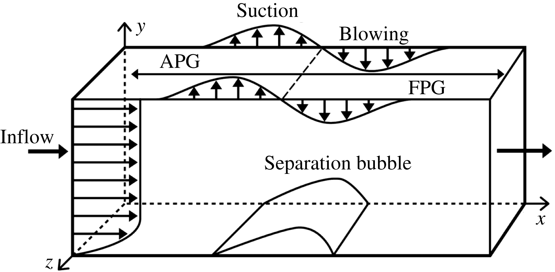
Computational domain.

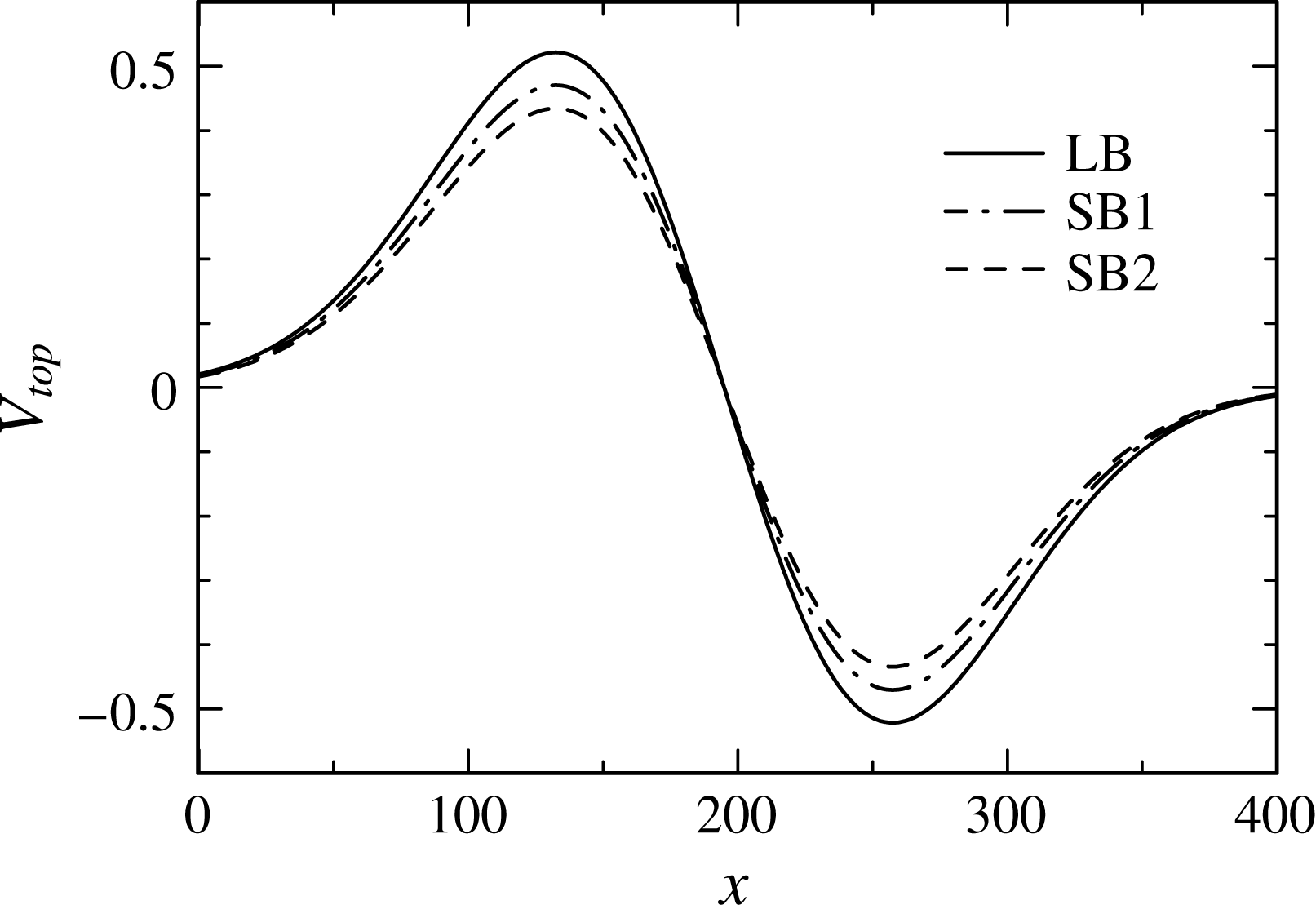
Transpiration velocity profile.

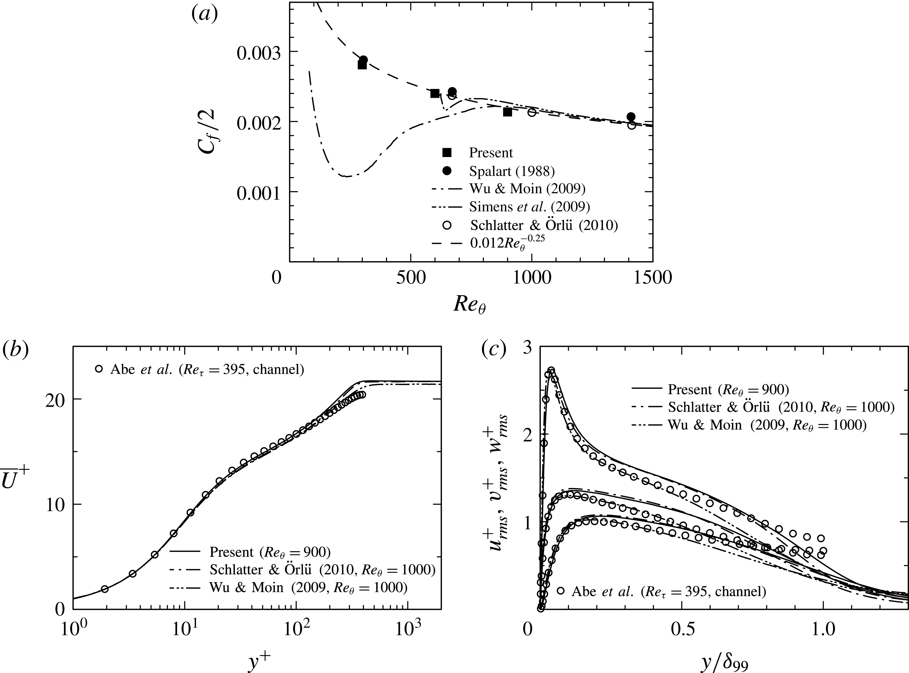
Mean and turbulence statistics at the inlet: (a)
 $C_{f}/2$
as a function of
 $Re_{\unicode[STIX]{x1D703}}$
; (b)
 $\overline{U}^{+}$
for
 $Re_{\unicode[STIX]{x1D703}}=900$
; (c)
 $u_{rms}^{+}$
,
 $v_{rms}^{+}$
,
 $w_{rms}^{+}$
for
 $Re_{\unicode[STIX]{x1D703}}=900$
.

2 DNS set-up
The computational domain is shown in figure 1 where
 $x$
,
 $y$
and
 $z$
denote the streamwise, wall-normal and spanwise directions, respectively. Throughout the paper, all variables are normalized by the inlet free stream velocity
 $U_{0}$
and momentum thickness
 $\unicode[STIX]{x1D703}_{0}$
unless otherwise stated. A two-dimensional separation bubble is considered so that the periodic boundary condition is used in the
 $z$
direction. As in Spalart & Coleman (Reference Spalart and Coleman1997) and Na & Moin (Reference Na and Moin1998a
,Reference Na and Moin
b
), the suction and blowing are imposed at the upper boundary to have a separation bubble, while a no-slip condition is used at the wall. The present transpiration velocity is given by
 $$\begin{eqnarray}\displaystyle V_{top}=V_{max}\times \sqrt{2}\times \left(\frac{x_{c}-x}{\unicode[STIX]{x1D70E}}\right)\exp \left(\unicode[STIX]{x1D713}-\left(\frac{x_{c}-x}{\unicode[STIX]{x1D70E}}\right)^{2}\right), & & \displaystyle\end{eqnarray}$$
with
 $V_{max}=0.3325$
,
 $x_{c}=10^{5}/2^{9}$
,
 $\unicode[STIX]{x1D70E}=80\sqrt{2}$
,
 $\unicode[STIX]{x1D6F9}=0.95$
; the resulting profile is given in figure 2 (denoted as LB) where maximum values of the suction and blowing are by about 20 per cent larger than those of Spalart & Coleman (Reference Spalart and Coleman1997) (denoted as SB2) to have massive separation. As for boundary conditions for other velocity components at this location, a zero spanwise vorticity condition, viz.
 $$\begin{eqnarray}\displaystyle \unicode[STIX]{x1D6FA}_{z}=\frac{\unicode[STIX]{x2202}V}{\unicode[STIX]{x2202}x}-\frac{\unicode[STIX]{x2202}U}{\unicode[STIX]{x2202}y}=0, & & \displaystyle\end{eqnarray}$$
is used for
 $U$
, whereas the Neumann condition
 $\unicode[STIX]{x2202}W/\unicode[STIX]{x2202}y=0$
is for
 $W$
. Note that the earlier DNS (Abe et al.
Reference Abe, Mizobuchi, Matsuo and Spalart2012) used a large magnitude of
 $V_{top}$
. This however yields a stagnation point near the upper boundary, which is troublesome to have the long-time sampling. The present DNS (Abe et al.
Reference Abe, Mizobuchi, Matsuo and Spalart2015) therefore adopts small
 $V_{top}$
and wall-normal domain size
 $L_{y}$
to avoid the stagnation point. The agreement in basic statistics between the earlier (Abe et al.
Reference Abe, Mizobuchi, Matsuo and Spalart2012) and present (Abe et al.
Reference Abe, Mizobuchi, Matsuo and Spalart2015) DNS is satisfactory. A small difference appears in the recovery region, in which turbulence is reduced slightly in the present DNS. The inflow data prescribed are DNS data of a ZPG turbulent boundary layer, which are generated by the rescaling–recycling method (Lund, Wu & Squires Reference Lund, Wu and Squires1998) with a constant spanwise shift (Spalart, Strelets & Travin Reference Spalart, Strelets and Travin2006) to avoid possible periodicity of the inlet data. A convective boundary condition is used for the outlet. Three values of
 $Re_{\unicode[STIX]{x1D703}}$
(=300, 600 and 900) are used. The corresponding
 $Re_{\unicode[STIX]{x1D70F}}(\equiv U_{\unicode[STIX]{x1D70F}}\unicode[STIX]{x1D6FF}_{99}/\unicode[STIX]{x1D708})$
is equal to 140, 250 and 350 (
 $U_{\unicode[STIX]{x1D70F}}$
and
 $\unicode[STIX]{x1D6FF}_{99}$
denote the friction velocity and 99 % boundary layer thickness, respectively). Distributions of friction coefficient
 $C_{f}\equiv 2/U_{0}^{+2}$
, mean streamwise velocity
 $\overline{U}^{+}$
and r.m.s. values of velocity fluctuations
 $u_{rms}^{+}$
,
 $v_{rms}^{+}$
,
 $w_{rms}^{+}$
at the inlet are shown in figure 3 (note that an upper case denotes the mean quantity; a superscript
 $+$
normalization by wall units). Overall agreement with the existing DNS of a ZPG turbulent boundary layer (Spalart Reference Spalart1988; Simens et al.
Reference Simens, Jiménez, Hoyas and Mizuno2009; Wu & Moin Reference Wu and Moin2009; Schlatter & Örlü Reference Schlatter and Örlü2010) is satisfactory.
Numerical methodology is briefly as follows. The current DNS code has been developed based on the channel DNS code (Abe, Kawamura & Matsuo Reference Abe, Kawamura and Matsuo2004). A fractional step method is used with semi-implicit time advancement. The Crank–Nicolson method is used for the viscous terms in the
 $y$
direction, and the third-order Runge–Kutta method is used for the other terms. A finite difference method is used as a spatial discretization. A fourth-order central scheme (Morinishi et al.
Reference Morinishi, Lund, Vasilyev and Moin1998) is used in the
 $x$
and
 $z$
directions, whilst a second-order central scheme is used in the
 $y$
direction. The computational domain size (
 $L_{x}\times L_{y}\times L_{z}$
), number of grid points (
 $N_{x}\times N_{y}\times N_{z}$
), spatial resolution at the inlet (
 $\unicode[STIX]{x0394}x_{0}$
,
 $\unicode[STIX]{x0394}y_{0}$
,
 $\unicode[STIX]{x0394}z_{0}$
) and sampling time period (
 $T$
) are given in table 1. A uniform grid is used in the
 $x$
and
 $z$
directions, while a non-uniform grid is in the
 $y$
direction (the latter grid is clustered both near the wall and the upper boundary but stretched towards
 $L_{y}/2$
). The present DNS uses a relatively large spanwise domain to prevent an artificial constraint to large-scale structures existing in the separated shear layer and recovery region (see Abe et al.
Reference Abe, Mizobuchi, Matsuo and Spalart2012). Once the velocity field reaches the fully developed and statistically steady state (i.e. time-independent profiles of
 $C_{f}$
and
 $C_{p}(\equiv 2(P_{w}-P_{w,0}))$
), the Navier–Stokes equations are integrated further in time to obtain mean quantities and second moments of velocity fluctuations and their budgets.
Domain size, grid points, spatial resolution and sampling time period.

In § 3.1, we also examine effects of varying
 $V_{top}$
(i.e. pressure gradients) with focus on similarities/differences between incipient and massive separation. This will be done by testing three different magnitudes of
 $V_{top}$
for
 $Re_{\unicode[STIX]{x1D703}}=300$
, where the present transpiration velocity
 $V_{top}$
(LB) is reduced down to the value of Spalart & Coleman (Reference Spalart and Coleman1997) (see figure 2 where the magnitude of SB1 (
 $V_{max}=0.300$
) is 10 % smaller than LB, while that of SB2 (
 $V_{max}=0.277$
) (equivalent to the value of Spalart & Coleman (Reference Spalart and Coleman1997)) is approximately 20 % smaller than LB). Note that domain size, number of grid points, spatial resolution and sampling time period for SB1 and SB2 are the same as for LB (see table 1). On the other hand, effects of the Reynolds number are examined in § 3.2 with the use of three datasets for
 $Re_{\unicode[STIX]{x1D703}}=300$
,
 $600$
and
 $900$
obtained with the largest
 $V_{top}$
(LB).
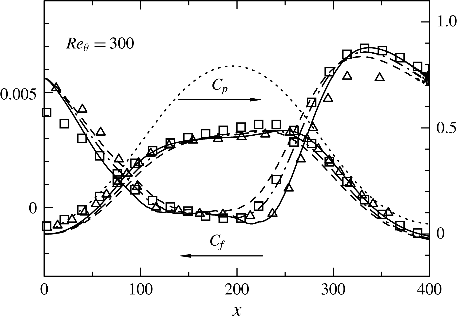
Distributions of
 $C_{f}$
and
 $C_{p}$
for
 $Re_{\unicode[STIX]{x1D703}}=300$
obtained with three different magnitudes of
 $V_{top}$
. ——, LB; — ⋅ —, SB1; – – –, SB2;
 $\cdots \cdots$
, inviscid
 $C_{p}$
; ▫, Spalart & Coleman (Reference Spalart and Coleman1997); ▵, Na & Moin (Reference Na and Moin1998b
).

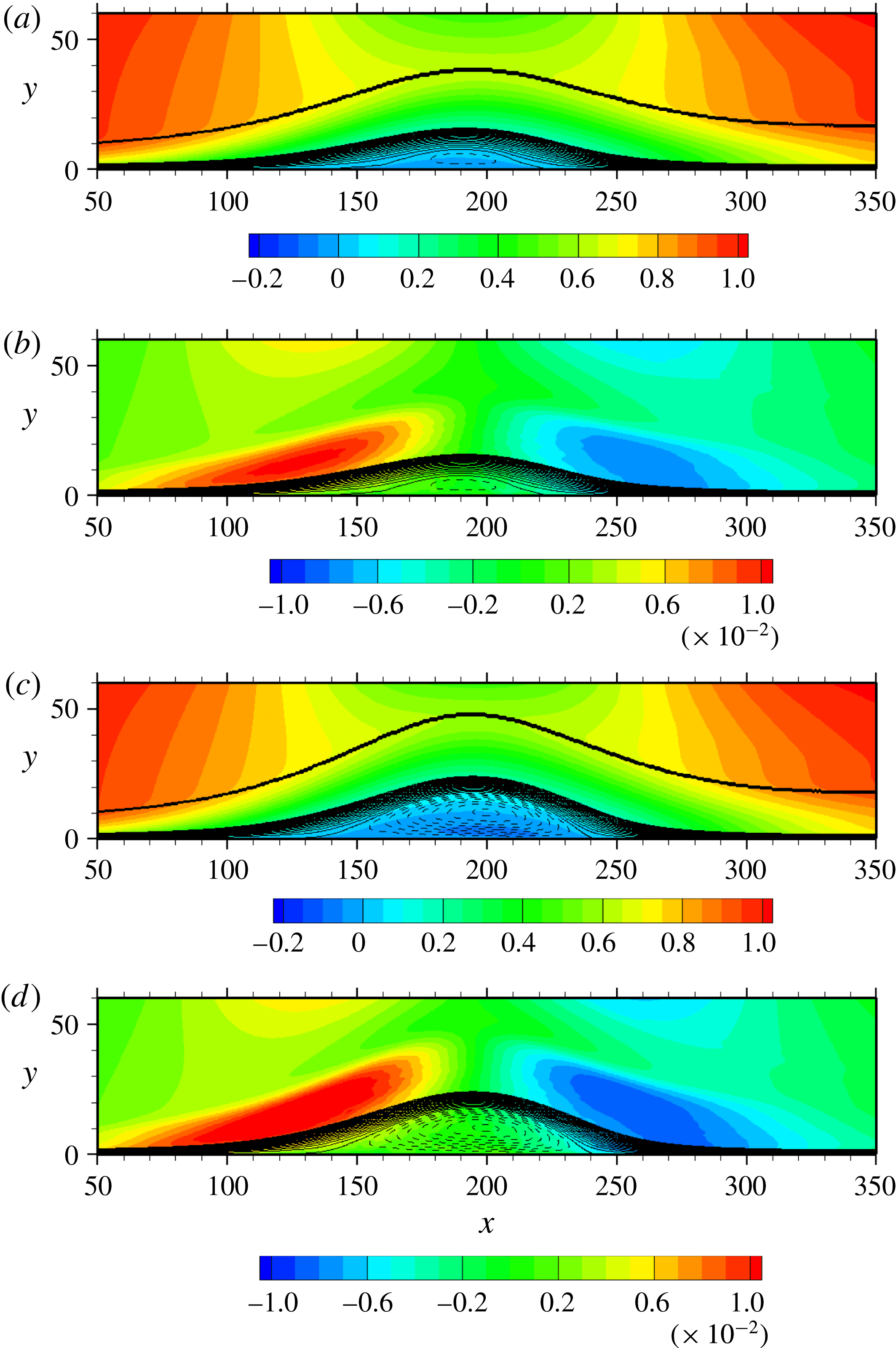
Contours of
 $\overline{U}/U_{0}$
and
 $\unicode[STIX]{x2202}\overline{V}/\unicode[STIX]{x2202}y$
for
 $Re_{\unicode[STIX]{x1D703}}=300$
obtained with different magnitudes of
 $V_{top}$
: (a)
 $\overline{U}/U_{0}$
(SB1); (b)
 $(\unicode[STIX]{x2202}\overline{V}/\unicode[STIX]{x2202}y)/(U_{0}/\unicode[STIX]{x1D703}_{0})$
(SB1); (c)
 $\overline{U}/U_{0}$
(LB); (d)
 $(\unicode[STIX]{x2202}\overline{V}/\unicode[STIX]{x2202}y)/(U_{0}/\unicode[STIX]{x1D703}_{0})$
(LB). Solid and dashed lines denote positive and negative streamlines, respectively. In (a) and (c), the bold line denotes the 99 % boundary layer thickness, which is obtained with the pseudo-velocity
 $\overline{U}(y)=-\!\int _{0}^{y}\overline{\unicode[STIX]{x1D6FA}}_{z}(y^{\prime })\,\text{d}y^{\prime }$
.

3 Results on wall-pressure fluctuations
3.1 Effects of varying transpiration velocity
 $V_{top}$

We first examine effects of varying
 $V_{top}$
regarding basic mean and turbulence quantities and the relationship with
 $p_{w}$
. Distributions of
 $C_{f}$
and
 $C_{p}$
obtained with three different magnitudes of
 $V_{top}$
are given in figure 4 for
 $Re_{\unicode[STIX]{x1D703}}=300$
, as compared with those of Spalart & Coleman (Reference Spalart and Coleman1997) for incipient separation and those of Na & Moin (Reference Na and Moin1998b
) for massive separation. In this figure, the inviscid wall-pressure distribution is also included. As noted in § 2, the current DNS imposes the same magnitude of suction and blowing (viz. APG and FPG) at the upper boundary. This leads to a symmetric inviscid wall-pressure distribution (see also the ‘bell-shaped’ distribution in Spalart & Coleman (Reference Spalart and Coleman1997)). Figure 4 demonstrates how the separated region is affected by varying
 $V_{top}$
. Clearly, the separation and reattachment points (i.e.
 $C_{f}=0$
) move upstream and downstream as the magnitude of
 $V_{top}$
increases. This is essentially associated with the increased APG and FPG (see distributions of
 $\unicode[STIX]{x2202}\overline{V}/\unicode[STIX]{x2202}y$
(or equivalently,
 $-\unicode[STIX]{x2202}\overline{U}/\unicode[STIX]{x2202}x$
, owing to the solenoidal condition, viz.
 $\unicode[STIX]{x2202}\overline{U}_{i}/\unicode[STIX]{x2202}x_{i}=0$
) in figure 5). The
 $C_{p}$
profile also changes with the magnitude of
 $V_{top}$
, i.e. the plateau tends to appear inside the bubble for the largest
 $V_{top}$
(LB) due to the presence of a dead water region. The present
 $C_{f}$
and
 $C_{p}$
distributions for the largest
 $V_{top}$
(LB) agree well with those of Na & Moin (Reference Na and Moin1998b
). The agreement with Spalart & Coleman (Reference Spalart and Coleman1997) is also satisfactory for the smallest
 $V_{top}$
(SB2) (note a discernible difference between the present study and that of Spalart & Coleman (Reference Spalart and Coleman1997) near inlet due to different inlet length).
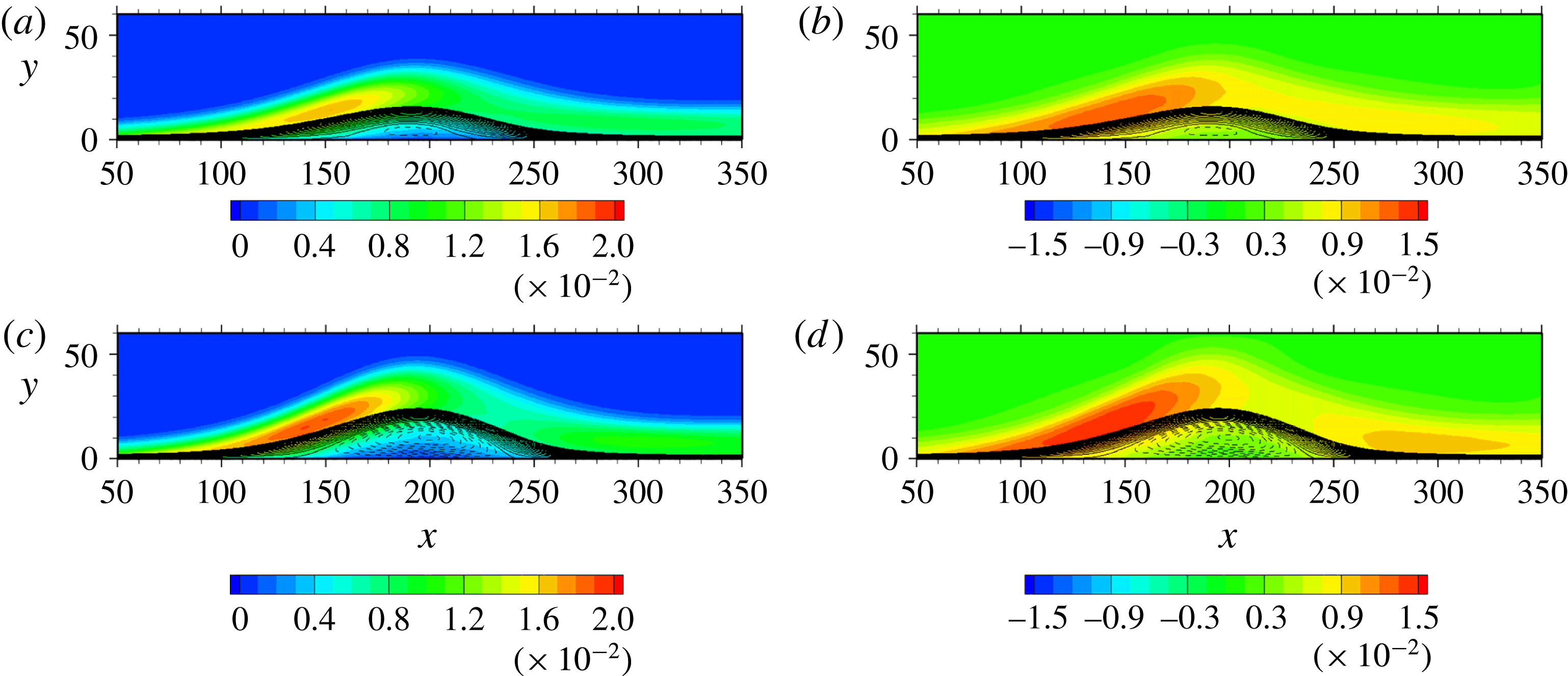
Contours of
 $k/U_{0}^{2}$
and
 $p_{rms}/\unicode[STIX]{x1D70C}U_{0}^{2}$
for
 $Re_{\unicode[STIX]{x1D703}}=300$
obtained with different magnitudes of
 $V_{top}$
: (a)
 $k/U_{0}^{2}$
(SB1); (b)
 $p_{rms}/\unicode[STIX]{x1D70C}U_{0}^{2}$
(SB1); (c)
 $k/U_{0}^{2}$
(LB); (d)
 $p_{rms}/\unicode[STIX]{x1D70C}U_{0}^{2}$
(LB). Solid and dashed lines denote positive and negative streamlines, respectively.

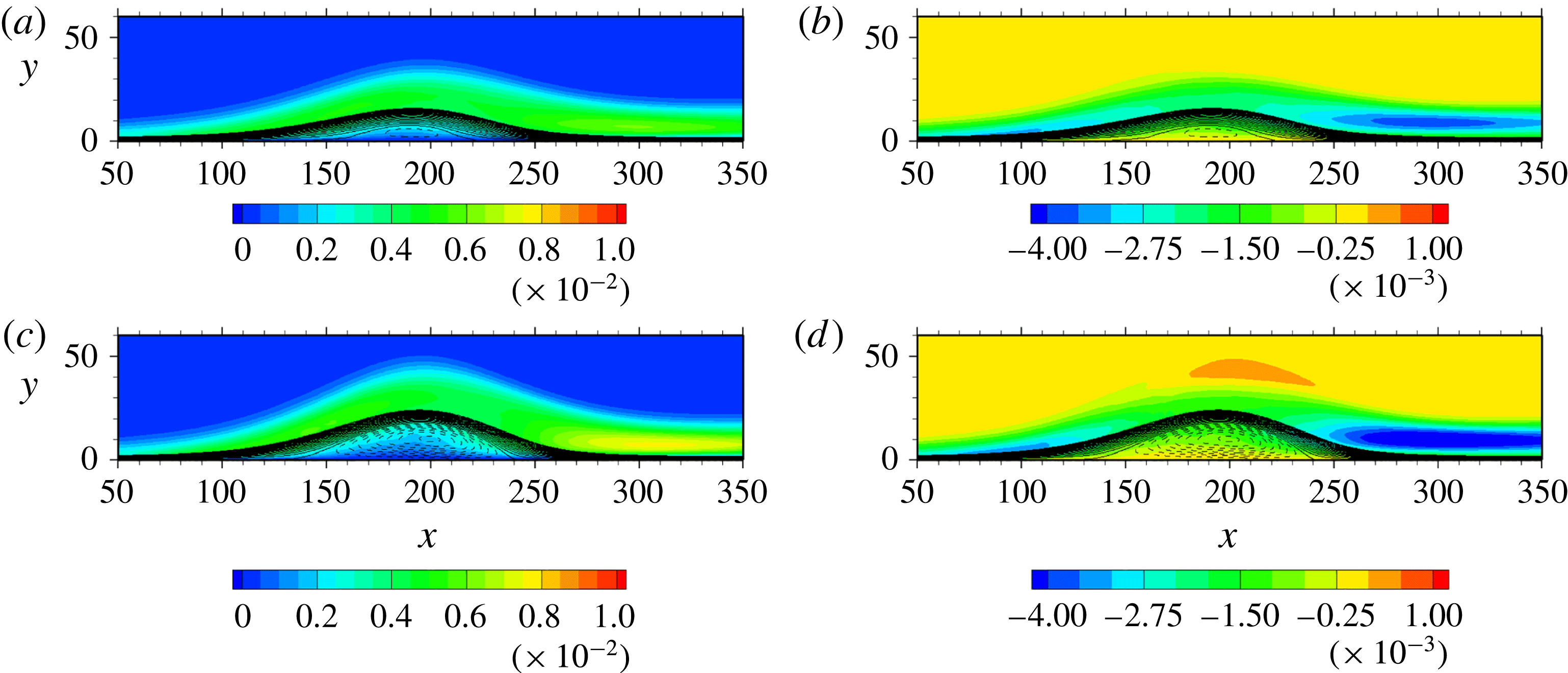
Contours of
 $\overline{vv}/U_{0}^{2}$
and
 $\overline{uv}/U_{0}^{2}$
for
 $Re_{\unicode[STIX]{x1D703}}=300$
obtained with different magnitudes of
 $V_{top}$
: (a)
 $\overline{vv}/U_{0}^{2}$
(SB1); (b)
 $\overline{uv}/U_{0}^{2}$
(SB1); (c)
 $\overline{vv}/U_{0}^{2}$
(LB); (d)
 $\overline{uv}/U_{0}^{2}$
(LB). Solid and dashed lines denote positive and negative streamlines, respectively.

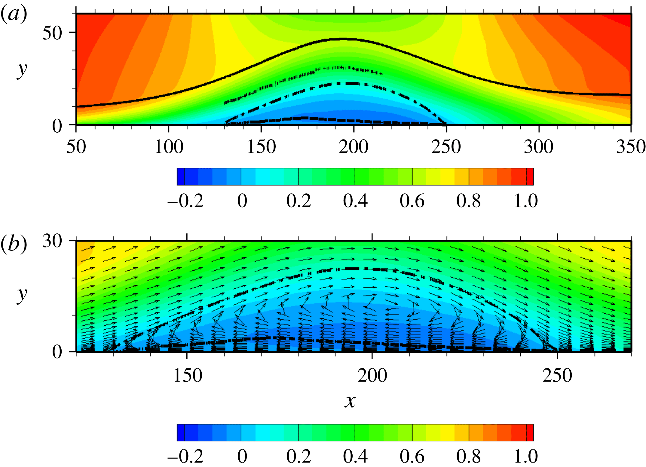
Figure 5 shows contours of mean streamwise velocity
 $\overline{U}/U_{0}$
in the
 $x{-}y$
plane together with those of
 $\unicode[STIX]{x2202}\overline{V}/\unicode[STIX]{x2202}y$
(or equivalently,
 $-\unicode[STIX]{x2202}\overline{U}/\unicode[STIX]{x2202}x$
), the latter exhibiting a degree of mean flow acceleration/deceleration. As the separation point is approached, the boundary layer thickness
 $\unicode[STIX]{x1D6FF}_{99}$
(see a bold line in figures 5
a and 5
c) becomes increasingly thickened due to the increased APG. The increase of
 $\unicode[STIX]{x1D6FF}_{99}$
is significant after separation especially for the largest
 $V_{top}$
(LB) (see also displacement of streamlines in figure 5). Whilst there is only a small recirculation region for the smallest
 $V_{top}$
(SB2) (the figure is not shown here), a significant backflow is observed inside the bubble for the largest
 $V_{top}$
(LB) (see figure 5
c). In the present simulations, the magnitude of
 $\unicode[STIX]{x2202}\overline{V}/\unicode[STIX]{x2202}y>0$
(or equivalently,
 $\unicode[STIX]{x2202}\overline{U}/\unicode[STIX]{x2202}x<0$
) increases with the magnitude of
 $V_{top}$
in the APG and separated regions (i.e.
 $x<195$
). At the same time, the magnitude of
 $\unicode[STIX]{x2202}\overline{V}/\unicode[STIX]{x2202}y<0$
(or equivalently,
 $\unicode[STIX]{x2202}\overline{U}/\unicode[STIX]{x2202}x>0$
) increases with the magnitude of
 $V_{top}$
in the FPG and reattached regions (i.e.
 $x>195$
). Alving & Fernholz (Reference Alving and Fernholz1996) also noted that
 $\unicode[STIX]{x2202}\overline{V}/\unicode[STIX]{x2202}y<0$
is required for closing the bubble in their measurement of an incipient turbulent separation bubble. The present flow is thus not only decelerated in the separated region, but also accelerated in the reattached region. The magnitude of the pressure-gradient parameter
 $\unicode[STIX]{x1D6FD}\equiv (\unicode[STIX]{x1D6FF}^{\ast }/C_{f})(\unicode[STIX]{x2202}C_{p}/\unicode[STIX]{x2202}x)\approx 104$
(LB),
 $33$
(SB1) and
 $20$
(SB2) near separation (
 $x=100$
), while it is approximately
 $-4.5$
(LB),
 $-3.5$
(SB1),
 $-3.0$
(SB2) in the reattached region (
 $x=300$
), which underlines that the present flow is subjected to large pressure gradients.
Contours of turbulent kinetic energy
 $k/U_{0}^{2}$
and r.m.s. pressure fluctuations
 $p_{rms}/\unicode[STIX]{x1D70C}U_{0}^{2}$
for
 $Re_{\unicode[STIX]{x1D703}}=300$
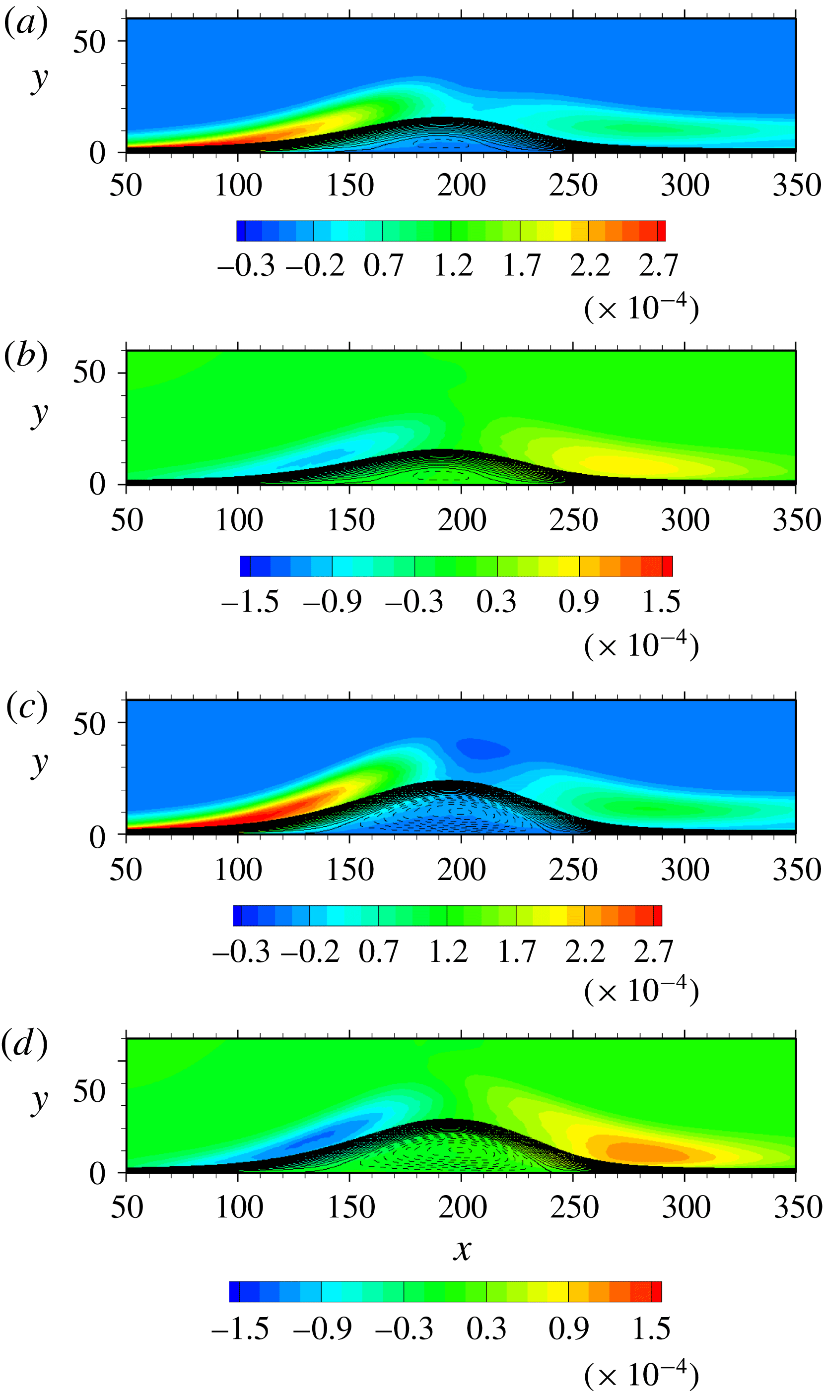
are given in figure 6 together with those of streamlines. The magnitude of
 $k/U_{0}^{2}$
increases with the
 $x$
location due to the increase of APG, i.e.
 $\unicode[STIX]{x2202}\overline{U}/\unicode[STIX]{x2202}x<0$
(or equivalently
 $\unicode[STIX]{x2202}\overline{V}/\unicode[STIX]{x2202}y>0$
) (see figures 5
b and 5
d). After separation, turbulence structures in an APG boundary layer are lifted above the separation bubble (see also figure 23 where contours of instantaneous streamwise velocity and pressure fluctuations are shown). The largest magnitude of
 $k/U_{0}^{2}$
appears in the separated shear layer (
 $x\approx 140$
), which increases with the magnitude of
 $V_{top}$
. This increased magnitude of
 $k/U_{0}^{2}$
essentially comes from those of
 $\overline{uu}$
and
 $\overline{ww}$
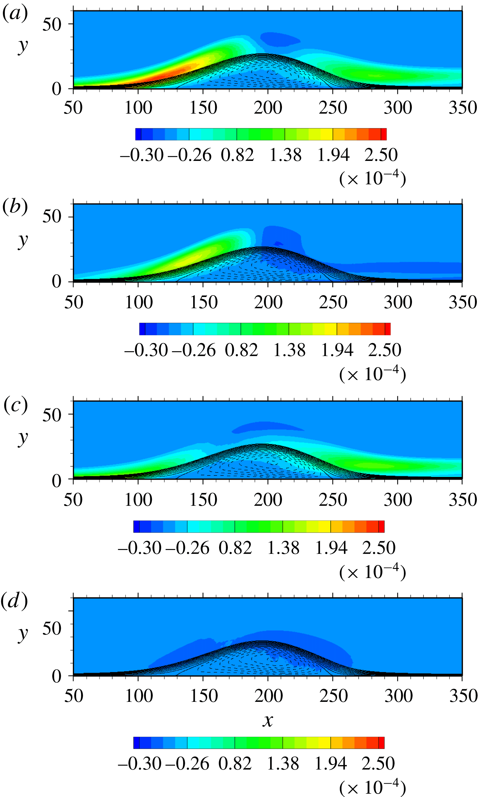
(not shown here), whilst the magnitudes of
 $\overline{vv}$
and
 $\overline{uv}$
remain almost unchanged independently of the magnitude of
 $V_{top}$
(see figure 7). This implies that in the separated shear layer the inactive motion contributes more significantly to the turbulent kinetic energy than the active motion. Note that the inactive motion refers to the large-scale motion and the irrotational pressure fluctuations of the outer region (Townsend Reference Townsend1961; Bradshaw Reference Bradshaw1967) which contribute to the Reynolds normal stress (mostly to the low wavenumber components of
 $\overline{uu}$
and
 $\overline{ww}$
as described by Townsend (Reference Townsend1976)’s attached eddy model) in the inner region, while the active motion contributes almost exclusively to the Reynolds shear stress in the inner region (see also § 6 of Antonia et al. (Reference Antonia, Teitel, Kim and Browne1992)). At near top of the bubble (
 $x\approx 210$
), the production exhibits a negative peak as shown in figures 14(a,c) and 15(a) (see also Spalart & Coleman Reference Spalart and Coleman1997; Skote & Henningson Reference Skote and Henningson2002; Abe et al.
Reference Abe, Mizobuchi, Matsuo and Spalart2012) due to a rapid pressure-driven change of the strain rate. The magnitude of
 $k/U_{0}^{2}$
then decreases at
 $x\approx 240$
, while again exhibiting the large magnitude in the shear layer after reattachment. This behaviour is associated with convective nature of a pressure-induced separation bubble in the reattached region (see the region of
 $\unicode[STIX]{x2202}\overline{V}/\unicode[STIX]{x2202}y<0$
in figures 5
b and 5
d). The similar trend is evident in
 $p_{rms}/\unicode[STIX]{x1D70C}U_{0}^{2}$
. The present study highlights that while a large magnitude of
 $p_{rms}/\unicode[STIX]{x1D70C}U_{0}^{2}$
is generated in the separated shear layer (
 $x\approx 150$
), it decreases after the top of the bubble, but again exhibits a peak in the shear layer after reattachment. In the reattached region, the magnitude of
 $p_{rms}/\unicode[STIX]{x1D70C}U_{0}^{2}$
increases with the magnitude of
 $V_{top}$
and thus FPG. The resulting mean flow acceleration, i.e.
 $\unicode[STIX]{x2202}\overline{U}/\unicode[STIX]{x2202}x>0$
(or equivalently,
 $\unicode[STIX]{x2202}\overline{V}/\unicode[STIX]{x2202}y<0$
), is also associated with delay of the peak after reattachment (see close relationship between the large value of
 $p_{rms}/\unicode[STIX]{x1D70C}U_{0}^{2}$
(figures 6
b and 6
d) and that of
 $\unicode[STIX]{x2202}\overline{V}/\unicode[STIX]{x2202}y>0$
(figures 5
b and 5
d) in the reattached region). This behaviour is essentially different from that in the backward facing step (see figure 14 of Le, Moin & Kim (Reference Le, Moin and Kim1997)) where large pressure fluctuations are invariably observed in the shear layer near reattachment. The difference is linked to that observed in
 $p_{w}$
between pressure-induced separation and step-induced one, as discussed below.
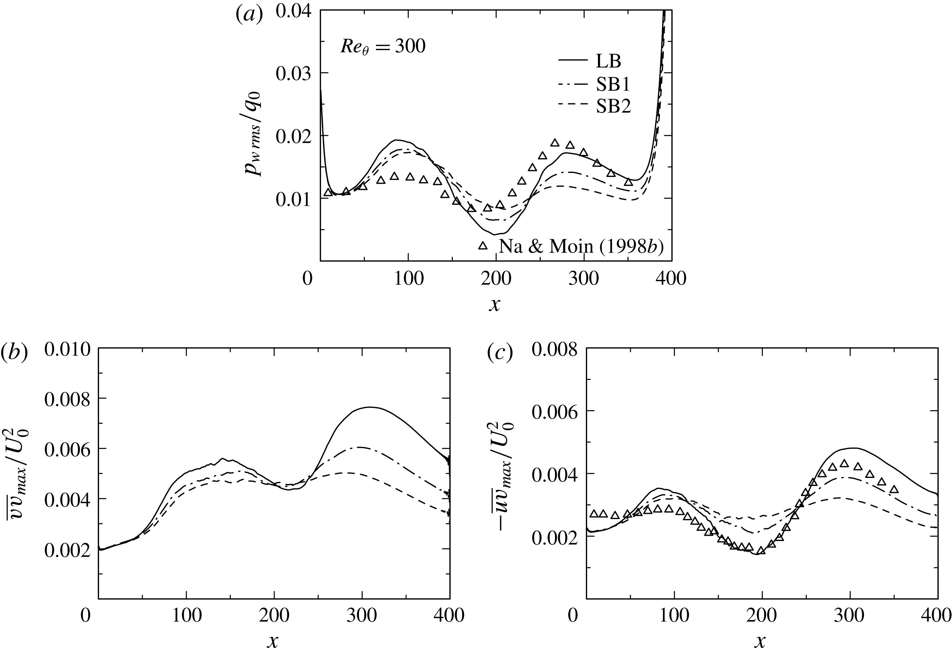
Distributions of
 $p_{w\,rms}/q_{0}$
,
 $\overline{vv}_{max}/U_{0}^{2}$
, and
 $-\overline{uv}_{max}/U_{0}^{2}$
for
 $Re_{\unicode[STIX]{x1D703}}=300$
obtained with three different magnitudes of
 $V_{top}$
: (a)
 $p_{w\,rms}/q_{0}$
; (b)
 $\overline{vv}_{max}/U_{0}^{2}$
; (c)
 $-\overline{uv}_{max}/U_{0}^{2}$
.

Figure 8(a) shows the r.m.s. value of wall-pressure fluctuations normalized by inlet dynamic pressure
 $p_{w\,rms}/q_{0}$
. Note that an abrupt increase of the present data both near inlet and outlet is due to effects of boundary conditions. While the largest magnitude of
 $p_{rms}/\unicode[STIX]{x1D70C}U_{0}^{2}$
is generated in the separated shear layer (
 $x\approx 150$
) (see figures 6
b and 6
d), the same trend is not observed for the wall-pressure fluctuations. In
 $p_{w\,rms}/q_{0}$
, a local peak appears near the separation point (
 $x\approx 100$
). This peak magnitude depends weakly on the magnitude of
 $V_{top}$
. In this context, an excellent similarity is observed for distributions between
 $p_{w\,rms}/q_{0}$
and
 $-\overline{uv}_{max}/U_{0}^{2}$
in the APG and separated regions (see figures 8
a and 8
c), as indicated by Simpson et al. (Reference Simpson, Ghodbane and Mcgrath1987) and Na & Moin (Reference Na and Moin1998b
). The present result underlines that vortical motion producing
 $-\overline{uv}$
(i.e. the active motion) makes an important contribution to
 $p_{w}$
in these regions. Note that a small difference is observed for distributions of
 $p_{w\,rms}/q_{0}$
and
 $-\overline{uv}_{max}/U_{0}^{2}$
near separation between the present study and that of Na & Moin (Reference Na and Moin1998b
), which may be due to different inlet conditions (i.e. spatial turbulent boundary layer data taken from the DNS of Spalart (Reference Spalart1988) were provided by invoking Taylor’s hypothesis in Na & Moin (Reference Na and Moin1998b
), while time advanced turbulent boundary layer data generated by the rescaling–recycling method (Lund et al.
Reference Lund, Wu and Squires1998) are in the present study). On the other hand, another peak appears in
 $p_{w\,rms}/q_{0}$
after the reattachment point. This peak
 $x$
location coincides well with that of
 $p_{rms}/\unicode[STIX]{x1D70C}U_{0}^{2}$
, which underlines close relationship between large pressure fluctuations above the wall and wall-pressure fluctuations. In the reattached region, both the magnitude and the peak
 $x$
location of
 $p_{w\,rms}/q_{0}$
increase with the magnitude of
 $V_{top}$
and thus FPG. As for the similarity between
 $p_{w\,rms}$
and
 $\overline{u_{i}u_{j}}$
, Mohammed-Taifour & Weiss (Reference Mohammed-Taifour and Weiss2016) noted that wall-pressure fluctuations near reattachment are associated with vertical velocity fluctuations in the shear layer close to the wall and that the
 $x$
location of
 $p_{w\,rms}/q_{0}$
corresponds to that of the maximum
 $\sqrt{\overline{v^{2}}}/U_{\infty }$
. Figure 8 highlights that a good similarity is observed not only for distributions between
 $p_{w\,rms}/q_{0}$
and
 $\overline{vv}_{max}/U_{0}^{2}$
, but also for those between
 $p_{w\,rms}/q_{0}$
and
 $-\overline{uv}_{max}/U_{0}^{2}$
in the reattached region. This is because near reattachment the shear layer involves mean flow acceleration (see the region of
 $\unicode[STIX]{x2202}\overline{V}/\unicode[STIX]{x2202}y<0$
in figures 5
b and 5
d) due to convective nature of a pressure-induced separation bubble so that both mean shear and mean normal stresses affect velocity and pressure fluctuations near reattachment (see the analysis in § 3.3 regarding a role of mean shear/normal stresses). In the next subsection, the resulting scaling law of
 $p_{w\,rms}$
will be discussed in comparison with that established for step-induced separation (Ji & Wang Reference Ji and Wang2012) where the magnitude of mean flow acceleration is small.
3.2 Reynolds-number dependence and scaling law of
$p_{w\,rms}$

Here, we first attempt to clarify the
 $Re$
dependence for a large separation bubble, i.e. the largest
 $V_{top}$
case (LB). Distributions of
 $C_{f}$
and
 $C_{p}$
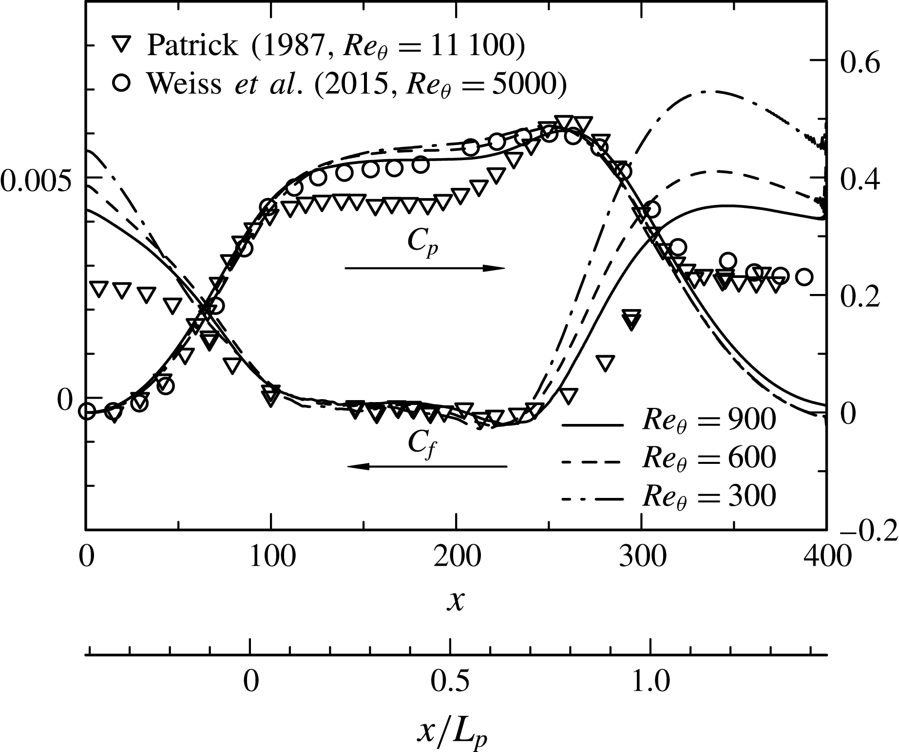
are given in figure 9 for
 $Re_{\unicode[STIX]{x1D703}}=300$
, 600 and 900. Also made is comparison with the experiments of Weiss et al. (Reference Weiss, Mohammed-Taifour and Schwaab2015) for
 $Re_{\unicode[STIX]{x1D703}}=5000$
and of Patrick (Reference Patrick1987) for
 $Re_{\unicode[STIX]{x1D703}}=11\,100$
. In the experiments of Patrick (Reference Patrick1987) and Weiss et al. (Reference Weiss, Mohammed-Taifour and Schwaab2015), a symmetric upper roof is used, which provides pressure gradients analogous to those in the present flow. The resulting
 $C_{p}$
distributions thus have strong resemblance between the present DNS and experiments outside the bubble (except for the outlet). Here, we introduce length scale
 $L_{p}$
to normalize the bubble, which is obtained by measuring two upstream and downstream stations that
 $C_{p}$
takes 0.3. Apparently, this normalization makes the
 $C_{p}$
distributions collapsed reasonably. Inside the bubble, the magnitude of
 $C_{p}$
decreases slightly with increasing
 $Re_{\unicode[STIX]{x1D703}}$
. This is interpreted as an enhanced viscid–inviscid interaction. One may also notice near plateau in the distribution of
 $C_{p}$
for higher
 $Re$
cases, indicating the presence of a dead water region. This plateau is likely to be dominated at high
 $Re_{\unicode[STIX]{x1D703}}$
(see Patrick Reference Patrick1987; Cheng, Pullin & Samtaney Reference Cheng, Pullin and Samtaney2015). A local peak appears for
 $C_{p}$
in the reattached region due to the flow impingement onto the wall. The noticeable Reynolds-number effect is seen for
 $C_{f}$
in the APG and recovery regions. In particular, the rate of decrease in
 $C_{f}$
with increasing
 $Re_{\unicode[STIX]{x1D703}}$
is twice as large in the recovery region as in the inlet region (see
 $x\approx 340$
in figure 9), which may be associated with weak development of near-wall turbulence after reattachment. The separation point (i.e. the upstream
 $C_{f}=0$
location) varies slightly from
 $x\approx 108$
(
 $Re_{\unicode[STIX]{x1D703}}=300$
) to
 $x\approx 114$
(
 $Re_{\unicode[STIX]{x1D703}}=900$
), whereas the reattachment point (i.e. the downstream
 $C_{f}=0$
location) from
 $x\approx 241$
(
 $Re_{\unicode[STIX]{x1D703}}=300$
) to
 $x\approx 251$
(
 $Re_{\unicode[STIX]{x1D703}}=900$
). This
 $Re$
dependence can also be discerned in the mean velocity distributions (figures 5
c, 10
a and 10
b) where the separation bubble becomes increasingly enlarged with increasing
 $Re_{\unicode[STIX]{x1D703}}$
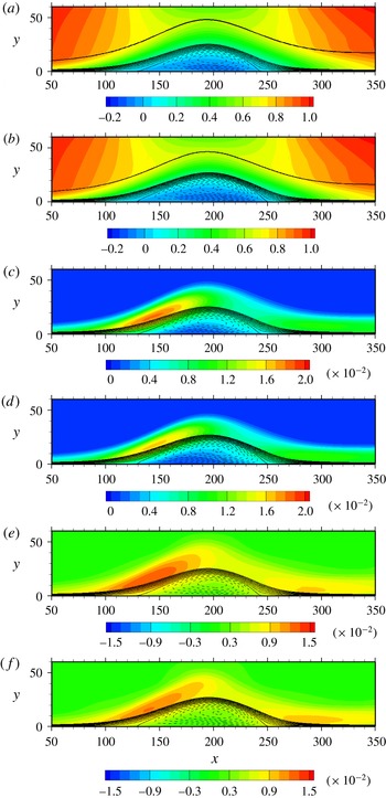
. On the other hand, the magnitudes of
 $k/U_{0}^{2}$
and
 $p_{rms}/\unicode[STIX]{x1D70C}U_{0}^{2}$
in the APG and separated regions decrease significantly with increasing
 $Re_{\unicode[STIX]{x1D703}}$
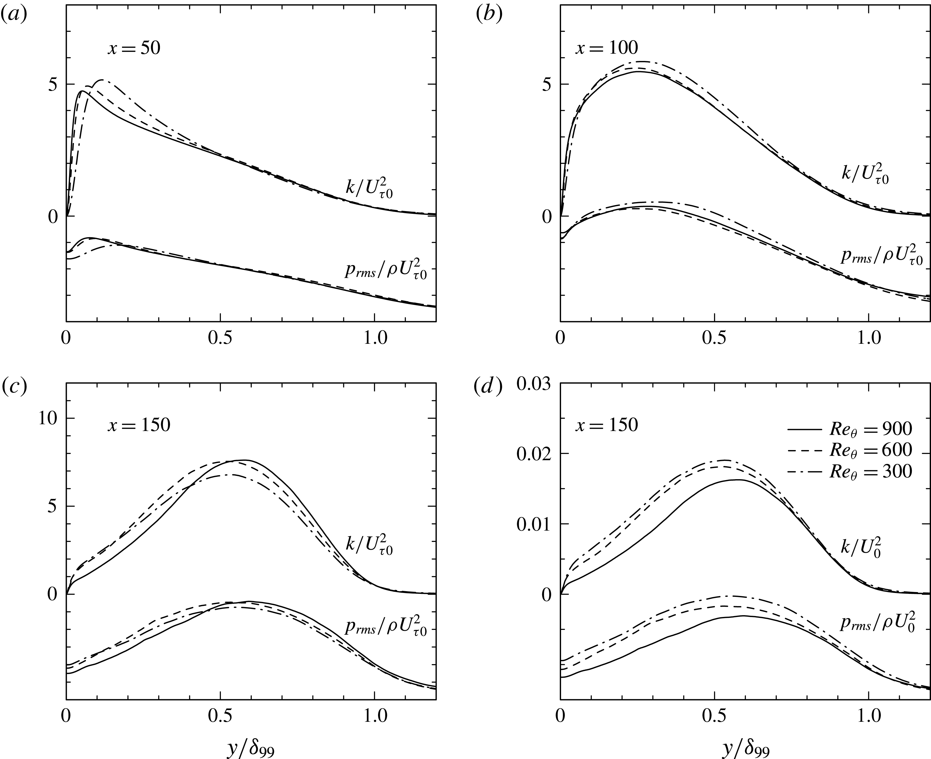
. This decrease is attributed to the
 $Re$
dependence of an incoming turbulent boundary layer. When normalization is made with the use of the inlet friction velocity
 $U_{\unicode[STIX]{x1D70F}0}(=U_{0}\sqrt{C_{f}/2})$
, good collapse is obtained in the outer part of a boundary layer near inlet (see figure 11
a where the distributions at
 $x=50$
are shown). This collapse is better observed in the downstream of an APG boundary layer (see figure 11
b), where peaks appear in the outer region. It is well established that velocity and pressure fluctuations show an outer peak in an APG turbulent boundary layer (see Lee & Sung Reference Lee and Sung2008). In the separated region, the collapse is still observed reasonably (see figures 11
c and 11
d), although the mixing layer scaling (see Abe et al.
Reference Abe, Mizobuchi, Matsuo and Spalart2012) seems to hold better than that on the basis of
 $U_{\unicode[STIX]{x1D70F}0}^{2}$
in this region. In the latter context, Song & Eaton (Reference Song and Eaton2004) noted that the collapse of
 $\overline{vv}/U_{\unicode[STIX]{x1D70F}0}^{2}$
is generally good in the separated region of a turbulent boundary layer over a contoured ramp for
 $Re_{\unicode[STIX]{x1D703}}=1100{-}20\,100$
. The analogous Reynolds-number dependence is also observed for
 $\overline{vv}$
and
 $\overline{uv}$
in the APG and separated regions (see figures 12
b and 12
c where distributions of
 $\overline{vv}_{max}/U_{0}^{2}$
and
 $-\overline{uv}_{max}/U_{0}^{2}$
are shown) in which normalization with
 $U_{\unicode[STIX]{x1D70F}0}^{2}$
yields good collapse (the distributions are not shown here). The present results highlight that effects of the active motion in an incoming boundary layer are dominated over the APG and separated regions and largely responsible for the
 $Re$
dependence. On the other hand, the magnitudes of
 $k/U_{0}^{2}$
and
 $p_{rms}/\unicode[STIX]{x1D70C}U_{0}^{2}$
remain invariably unchanged with increasing
 $Re_{\unicode[STIX]{x1D703}}$
in the reattached region, which depend substantially on FPG (see figures 6
b and 6
d).
Distributions of
 $C_{f}$
and
 $C_{p}$
for
 $Re_{\unicode[STIX]{x1D703}}=300$
,
 $600$
and
 $900$
. The data plotted in this figure have been obtained with the largest
 $V_{top}$
(LB).

Contours of
 $\overline{U}/U_{0}$
,
 $k/U_{0}^{2}$
and
 $p_{rms}/\unicode[STIX]{x1D70C}U_{0}^{2}$
for
 $Re_{\unicode[STIX]{x1D703}}=600$
(a,c,e) and
 $900$
(b,d,f): (a,b)
 $\overline{U}/U_{0}$
; (c,d)
 $k/U_{0}^{2}$
; (e,f)
 $p_{rms}/\unicode[STIX]{x1D70C}U_{0}^{2}$
. Solid and dashed lines denote positive and negative streamlines, respectively. The data plotted in this figure have been obtained with the largest
 $V_{top}$
(LB). In (a) and (b), the bold line denotes the 99 % boundary layer thickness, which is obtained with the pseudo-velocity
 $\overline{U}(y)=-\!\int _{0}^{y}\overline{\unicode[STIX]{x1D6FA}}_{z}(y^{\prime })\,\text{d}y^{\prime }$
.

Distributions of
 $k$
and
 $p_{rms}$
in the APG and separated regions with two different types of normalization for
 $Re_{\unicode[STIX]{x1D703}}=300$
,
 $600$
and
 $900$
: (a)
 $k/U_{\unicode[STIX]{x1D70F}0}^{2}$
and
 $p_{rms}/\unicode[STIX]{x1D70C}U_{\unicode[STIX]{x1D70F}0}^{2}$
(
 $x=50$
); (b)
 $k/U_{\unicode[STIX]{x1D70F}0}^{2}$
and
 $p_{rms}/\unicode[STIX]{x1D70C}U_{\unicode[STIX]{x1D70F}0}^{2}$
(
 $x=100$
); (c)
 $k/U_{\unicode[STIX]{x1D70F}0}^{2}$
and
 $p_{rms}/\unicode[STIX]{x1D70C}U_{\unicode[STIX]{x1D70F}0}^{2}$
(
 $x=150$
); (d)
 $k/U_{0}^{2}$
and
 $p_{rms}/\unicode[STIX]{x1D70C}U_{0}^{2}$
(
 $x=150$
). The data plotted in this figure have been obtained with the largest
 $V_{top}$
(LB).

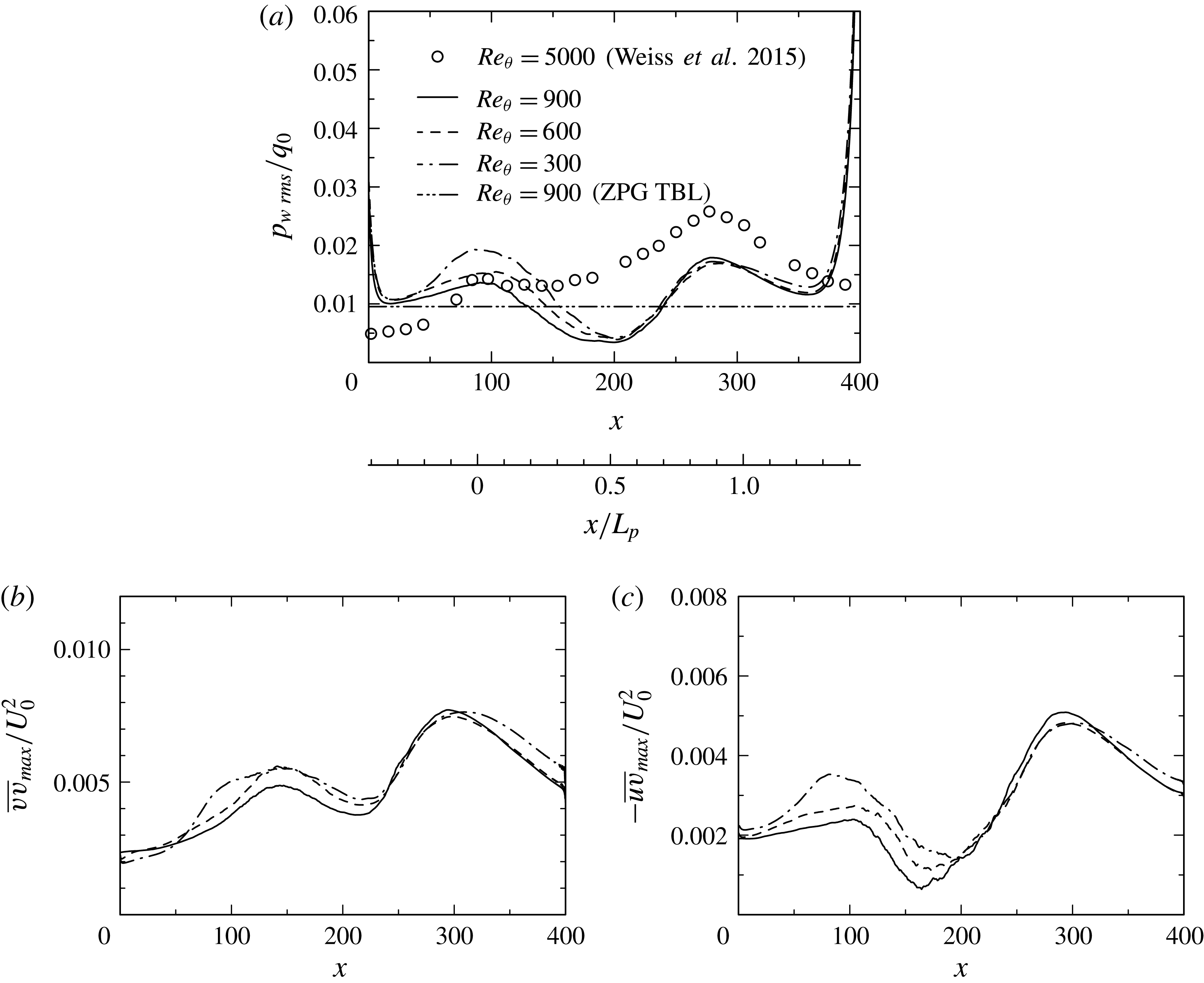
Figure 12 shows the r.m.s. value of wall-pressure fluctuations normalized by inlet dynamic pressure
 $p_{w\,rms}/q_{0}$
for
 $Re_{\unicode[STIX]{x1D703}}=300$
,
 $600$
and
 $900$
, as compared with those of Weiss et al. (Reference Weiss, Mohammed-Taifour and Schwaab2015) for
 $Re_{\unicode[STIX]{x1D703}}=5000$
. Clearly, this distribution is characterized by two local peaks. One is located near the separation point (
 $x\approx 100$
), while the other is after the reattachment point (
 $x\approx 280$
). The former peak has weak
 $Re$
dependence, which is also observed in the distributions of
 $-\overline{uv}_{max}/U_{0}^{2}$
and essentially associated with the active motion. On the other hand, the latter peak remains invariably unchanged for the three Reynolds numbers (i.e.
 $p_{w\,rms}/q_{0}=0.016$
). Indeed, the similarity between
 $p_{w\,rms}/q_{0}$
and
 $\overline{vv}_{max}/U_{0}^{2}$
and that between
 $p_{w\,rms}/q_{0}$
and
 $-\overline{uv}_{max}/U_{0}^{2}$
are convincing in the reattached region. Note that the peak magnitude of Weiss et al. (Reference Weiss, Mohammed-Taifour and Schwaab2015) is approximately 70 % larger than that of the present study. Given that FPG essentially affects wall-pressure fluctuations in the reattached region (see § 3.1), a larger magnitude of
 $p_{w\,rms}/q_{0}$
observed by Weiss et al. (Reference Weiss, Mohammed-Taifour and Schwaab2015) is attributed to larger FPG. The effects of FPG may not be dismissed in the reattached region of a pressure-induced separation bubble. We also stress that near reattachment the present magnitude of
 $p_{w\,rms}/q_{0}$
for the largest
 $V_{top}$
(LB) is twice smaller than that of a backward facing step (Le et al.
Reference Le, Moin and Kim1997), but about four times smaller than that of a forward facing step (Ji & Wang Reference Ji and Wang2012). This result underlines a discernible difference in the reattachment between pressure-induced separation and step-induced one.
Distributions of
 $p_{w\,rms}/q_{0}$
,
 $\overline{vv}_{max}/U_{0}^{2}$
and
 $-\overline{uv}_{max}/U_{0}^{2}$
for
 $Re_{\unicode[STIX]{x1D703}}=300$
,
 $600$
and
 $900$
: (a)
 $p_{w\,rms}/q_{0}$
; (b)
 $\overline{vv}_{max}/U_{0}^{2}$
; (c)
 $-\overline{uv}_{max}/U_{0}^{2}$
. The data plotted in this figure have been obtained with the largest
 $V_{top}$
(LB). In (a), the horizontal two-dotted line denotes a value of a ZPG turbulent boundary layer for
 $Re_{\unicode[STIX]{x1D703}}=900$
.

Distributions of
 $p_{w\,rms}/\unicode[STIX]{x1D70C}\overline{u_{i}u_{j}}_{max}$
for
 $Re_{\unicode[STIX]{x1D703}}=300$
,
 $600$
and
 $900$
: (a)
 $p_{w\,rms}/\unicode[STIX]{x1D70C}\overline{uu}_{max}$
; (b)
 $p_{w\,rms}/\unicode[STIX]{x1D70C}\overline{ww}_{max}$
; (c)
 $p_{w\,rms}/\unicode[STIX]{x1D70C}\overline{vv}_{max}$
; (d)
 $p_{w\,rms}/-\unicode[STIX]{x1D70C}\overline{uv}_{max}$
. The data plotted in this figure have been obtained for
 $Re_{\unicode[STIX]{x1D703}}=300$
with three different magnitudes of
 $V_{top}$
(i.e. SB1, SB2, LB) and for
 $Re_{\unicode[STIX]{x1D703}}=600$
and
 $900$
with the largest
 $V_{top}$
(LB). In each panel, the horizontal dashed line denotes a value of a ZPG turbulent boundary layer for
 $Re_{\unicode[STIX]{x1D703}}=900$
. In (a), an outer peak of
 $\overline{uu}$
has been considered as the maximum value in the APG and reattached regions.

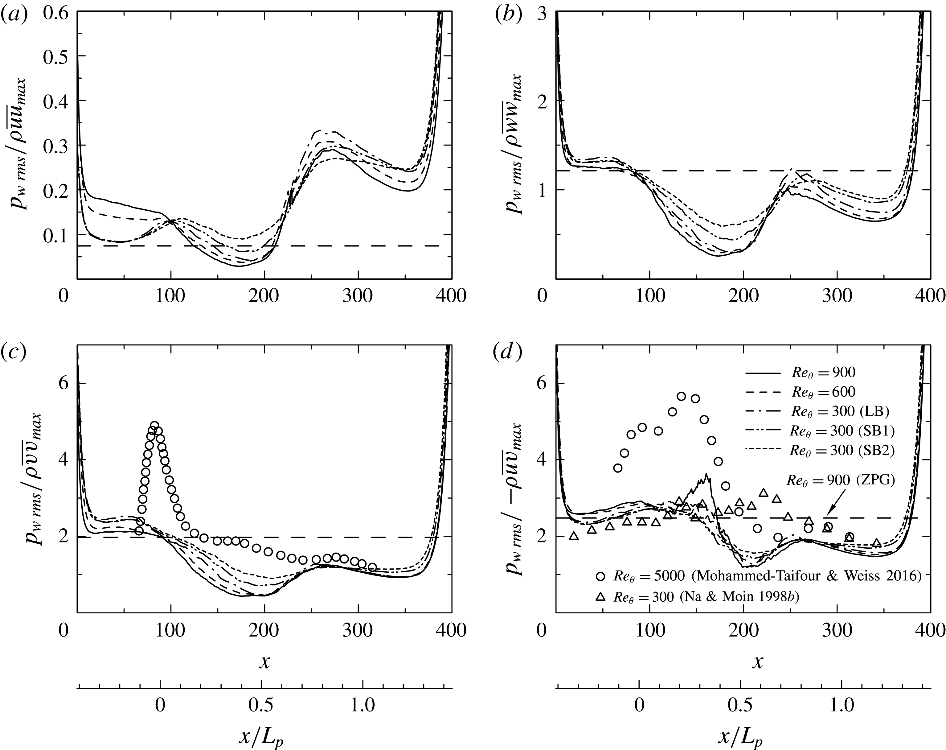
Now, we examine possible scaling laws of
 $p_{w\,rms}$
by testing normalization with the local maximum Reynolds stresses
 $\unicode[STIX]{x1D70C}\overline{u_{i}u_{j}}_{max}$
, as shown in figure 13. Indeed, the present data for
 $p_{w\,rms}/-\unicode[STIX]{x1D70C}\overline{uv}_{max}$
exhibit near plateau in the APG and separated regions with the magnitude of
 $2.5\sim 3$
for the three Reynolds numbers. The latter value agrees well with that of Na & Moin (Reference Na and Moin1998b
) for
 $Re_{\unicode[STIX]{x1D703}}=300$
. On the other hand, the experimental data (Simpson et al.
Reference Simpson, Ghodbane and Mcgrath1987; Mohammed-Taifour & Weiss Reference Mohammed-Taifour and Weiss2016) show considerably larger magnitudes than the DNS data (the present study; Na & Moin Reference Na and Moin1998b
). The reason for this difference is most likely due to measurement difficulties in
 $-\overline{uv}$
near separation since the later magnitude tends to attenuate gradually with increasing Reynolds number (see figure 12
c). The magnitude of
 $p_{w\,rms}/-\unicode[STIX]{x1D70C}\overline{uv}_{max}$
is however reduced down to 1.8 near reattachment where
 $p_{w\,rms}$
collapses not only on
 $-\unicode[STIX]{x1D70C}\overline{uv}_{max}$
but also on
 $\unicode[STIX]{x1D70C}\overline{vv}_{max}$
. Indeed, the magnitude of
 $p_{w\,rms}/\unicode[STIX]{x1D70C}\overline{vv}_{max}$
attains 1.2 unambiguously near reattachment independent of the magnitude of FPG (see figure 13
c where there is reasonable collapse between the present data (both the incipient and massive separation cases) and those of Mohammed-Taifour & Weiss (Reference Mohammed-Taifour and Weiss2016)). Note that a flat-plate turbulent boundary layer with separation and reattachment is not a canonical flow due largely to pressure gradients. In this context, Ji & Wang (Reference Ji and Wang2012) demonstrated that while a smaller step height results in large values of
 $p_{w\,rms}/\unicode[STIX]{x1D70C}\overline{vv}_{max}$
, the magnitude approaches 1.35 as the step height increases in the rear part of the recirculation bubble and further downstream. The present value of
 $p_{w\,rms}/\unicode[STIX]{x1D70C}\overline{vv}_{max}$
(1.2) is indeed smaller than (1.35) of Ji & Wang (Reference Ji and Wang2012) owing to a discernible difference in the reattachment between pressure-induced separation and step-induced one. In the present flow, negative production of
 $k$
arises at near top of the bubble (see figures 14
a, 14
c and 15
a) due to a rapid change of the mean strain rate (see Abe et al.
Reference Abe, Mizobuchi, Matsuo and Spalart2012). After this region, turbulence is developing slowly until reattachment, while convection is dominated (see figures 5
b, 5
d and 16
f where distributions of
 $\unicode[STIX]{x2202}\overline{V}/\unicode[STIX]{x2202}y$
are shown). This behaviour is essentially different from that of step-induced separation where turbulence keep developing until reattachment. We stress that mean flow acceleration resulting from FPG, i.e.
 $\unicode[STIX]{x2202}\overline{U}/\unicode[STIX]{x2202}x>0$
(or equivalently,
 $\unicode[STIX]{x2202}\overline{V}/\unicode[STIX]{x2202}y<0$
), is involved in the shear layer near reattachment of a pressure-induced separation bubble. The role of mean normal stress (i.e.
 $\unicode[STIX]{x2202}\overline{V}/\unicode[STIX]{x2202}y$
) will be further discussed in § 3.3 in the context of production of
 $\overline{u_{i}u_{j}}$
as compared with that of mean shear stress (i.e.
 $\unicode[STIX]{x2202}\overline{U}/\unicode[STIX]{x2202}y$
).
Contours of
 $P_{k}$
and
 $P_{22}$
normalized by
 $U_{0}^{3}/\unicode[STIX]{x1D703}_{0}$
for
 $Re_{\unicode[STIX]{x1D703}}=300$
obtained with different magnitudes of
 $V_{top}$
: (a)
 $P_{k}\unicode[STIX]{x1D703}_{0}/U_{0}^{3}$
(SB1); (b)
 $P_{22}\unicode[STIX]{x1D703}_{0}/U_{0}^{3}$
(SB1); (c)
 $P_{k}\unicode[STIX]{x1D703}_{0}/U_{0}^{3}$
(LB); (d)
 $P_{22}\unicode[STIX]{x1D703}_{0}/U_{0}^{3}$
(LB). Solid and dashed lines denote positive and negative streamlines, respectively.

3.3 Role of mean normal/shear stresses
In this subsection, we focus on the production for
 $\overline{u_{i}u_{j}}$
consisting of the product of Reynolds stress and mean velocity gradient, i.e.
 $$\begin{eqnarray}\displaystyle P_{ij}=-\overline{u_{i}u_{i}}\left(\frac{\unicode[STIX]{x2202}\bar{U}_{i}}{\unicode[STIX]{x2202}x_{j}}+\frac{\unicode[STIX]{x2202}\bar{U}_{j}}{\unicode[STIX]{x2202}x_{i}}\right), & & \displaystyle\end{eqnarray}$$
to gain further insights into the scaling laws of
 $p_{w\,rms}/\unicode[STIX]{x1D70C}\overline{vv}_{max}$
and
 $p_{w\,rms}/-\unicode[STIX]{x1D70C}\overline{uv}_{max}$
. Figure 14 demonstrates how the production terms for
 $k$
 $(P_{k}=P_{ii}/2)$
and
 $\overline{vv}$
 $(P_{22})$
vary with increasing the magnitude of
 $V_{top}$
. Clearly,
 $P_{k}$
increases significantly in the separated shear layer as the magnitude of
 $V_{top}$
increases (see figures 14
a and 14
c). This is due to the increased APG, consistent with the significant increase of
 $k/U_{0}^{2}$
in the separated shear layer (see figures 6
a and 6
c). This situation is however changed after the top of the bubble where there is convex streamline curvature and a change of the mean strain rate. In particular, the negative production arises noticeably when the separation bubble is large. After this region, turbulence is developing slowly, while convection is dominated (see figure 5). In the reattached region,
 $P_{k}$
again exhibits a peak after reattachment. This peak location moves downstream with increasing the magnitude of
 $V_{top}$
and thus FPG. The same trend is also observed for
 $P_{22}$
(see figure 14). Effects of FPG cannot be dismissed in the reattached region of the present flow.
Contours of the turbulent kinetic energy production normalized by
 $U_{0}^{3}/\unicode[STIX]{x1D703}_{0}$
for
 $Re_{\unicode[STIX]{x1D703}}=900$
: (a) total production (
 $P_{k}$
); (b) normal production; (c) shear production; (d) curvature production. Solid and dashed lines denote positive and negative streamlines, respectively. The data plotted in this figure have been obtained with the largest
 $V_{top}$
(LB).

Here, we examine a role of mean normal/shear stresses in the production of
 $\overline{u_{i}u_{j}}$
. In this context, Simpson, Chew & Shivaprasad (Reference Simpson, Chew and Shivaprasad1981) examined production terms of the transport equation for
 $k$
, viz.
 $$\begin{eqnarray}\displaystyle P_{k}=(\overline{vv}-\overline{uu})\frac{\unicode[STIX]{x2202}\bar{U}}{\unicode[STIX]{x2202}x}-\overline{uv}\left(\frac{\unicode[STIX]{x2202}\bar{U}}{\unicode[STIX]{x2202}y}+\frac{\unicode[STIX]{x2202}\bar{V}}{\unicode[STIX]{x2202}x}\right), & & \displaystyle\end{eqnarray}$$
in a massively separated open turbulent bubble (note that (3.2) is obtained from (3.1) with the use of the solenoidal condition). Equation (3.2) consists of normal (first and second terms), shear (third term) and curvature (fourth term) production terms. Simpson et al. (Reference Simpson, Chew and Shivaprasad1981) showed that the normal production terms are significant in the separated shear layer. Alving & Fernholz (Reference Alving and Fernholz1996) support the finding of Simpson et al. (Reference Simpson, Chew and Shivaprasad1981) in a mild turbulent separation bubble. Figure 15 shows the present distributions of (3.2) for
 $Re_{\unicode[STIX]{x1D703}}=900$
for the largest
 $V_{top}$
case (LB), which highlights the presence of negative
 $P_{k}$
even at large
 $Re_{\unicode[STIX]{x1D703}}$
. Clearly, the normal production contributes significantly to
 $P_{k}$
in the separated shear layer, whereas the shear production does to
 $P_{k}$
in both the separated and reattached regions. Note that the curvature production (i.e.
 $\unicode[STIX]{x2202}\overline{V}/\unicode[STIX]{x2202}x$
is an indicator of curvature (Bradshaw Reference Bradshaw1973)) is negligibly small except near top of the bubble (see also the curvature effect reported by Abe et al. (Reference Abe, Mizobuchi, Matsuo and Spalart2012)). In the separated shear layer, a large positive value of the normal production comes from the second term (i.e.
 $-\overline{uu}\unicode[STIX]{x2202}\overline{U}/\unicode[STIX]{x2202}x$
) of
 $k$
, which is a part of the production of
 $(P_{11})$
. On the other hand, the first term (i.e.
 $\overline{vv}\unicode[STIX]{x2202}\overline{U}/\unicode[STIX]{x2202}x$
), which is a part of the production of
 $(P_{22})$
(i.e. the second term in the right of (3.3) after use of the continuity equation), yields a negative value. The relative contribution of the normal stress
 $\unicode[STIX]{x2202}\overline{U}/\unicode[STIX]{x2202}x$
(or equivalently
 $-\unicode[STIX]{x2202}\overline{V}/\unicode[STIX]{x2202}y$
) however changes in the reattached region since the mean pressure gradient varies from APG to FPG after the top of the bubble (see figures 5
b and 5
d).
Contours of
 $\overline{uv}$
and
 $\overline{vv}$
, their production terms
 $P_{12}$
and
 $P_{22}$
and mean velocity gradients
 $\unicode[STIX]{x2202}\overline{U}/\unicode[STIX]{x2202}y$
and
 $\unicode[STIX]{x2202}\overline{V}/\unicode[STIX]{x2202}y$
for
 $Re_{\unicode[STIX]{x1D703}}=900$
: (a)
 $\overline{uv}/U_{0}^{2}$
; (b)
 $\overline{vv}/U_{0}^{2}$
; (c)
 $P_{12}\unicode[STIX]{x1D703}_{0}/U_{0}^{3}$
; (d)
 $P_{22}\unicode[STIX]{x1D703}_{0}/U_{0}^{3}$
; (e)
 $(\unicode[STIX]{x2202}\overline{U}/\unicode[STIX]{x2202}y)/(U_{0}/\unicode[STIX]{x1D703}_{0})$
; (f)
 $(\unicode[STIX]{x2202}\overline{V}/\unicode[STIX]{x2202}y)/(U_{0}/\unicode[STIX]{x1D703}_{0})$
. Solid and dashed lines denote positive and negative streamlines, respectively. The data plotted in this figure have been obtained with the largest
 $V_{top}$
(LB).

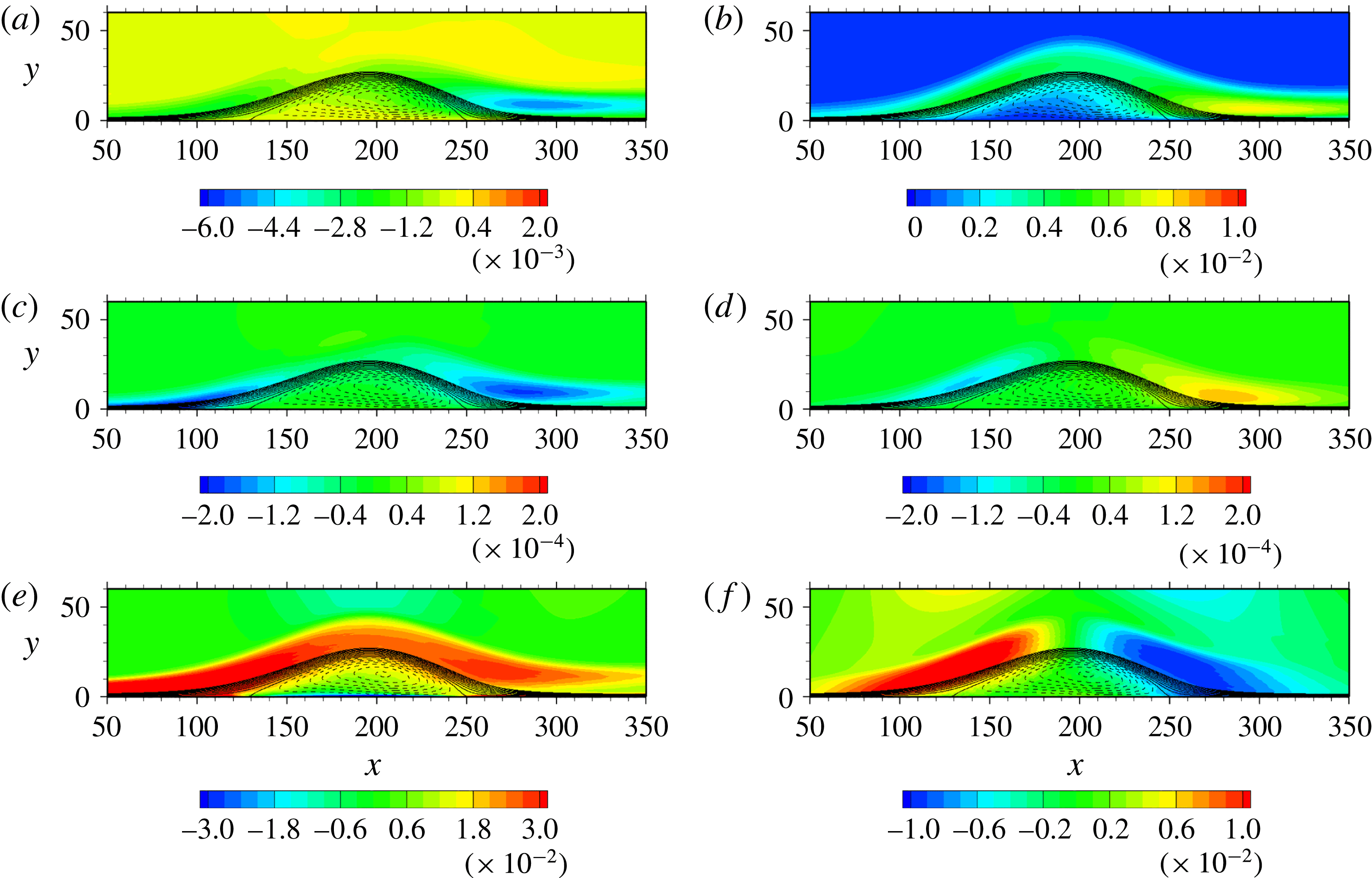
Figure 16 shows contours of the production for
 $\overline{vv}$
, viz.
 $$\begin{eqnarray}\displaystyle P_{22}=-2\overline{uv}\frac{\unicode[STIX]{x2202}\bar{V}}{\unicode[STIX]{x2202}x}-2\overline{vv}\frac{\unicode[STIX]{x2202}\bar{V}}{\unicode[STIX]{x2202}y}, & & \displaystyle\end{eqnarray}$$
and that for
 $\overline{uv}$
, viz.
 $$\begin{eqnarray}\displaystyle P_{12}=-\overline{vv}\frac{\unicode[STIX]{x2202}\bar{U}}{\unicode[STIX]{x2202}y}-\overline{uu}\frac{\unicode[STIX]{x2202}\bar{V}}{\unicode[STIX]{x2202}x}, & & \displaystyle\end{eqnarray}$$
for
 $Re_{\unicode[STIX]{x1D703}}=900$
. This figure highlights that the normal production (the second term in (3.3)) contributes significantly to
 $P_{22}$
near reattachment, whilst the shear production in
 $P_{22}$
(the first term in (3.3)) is negligibly small everywhere in the flow. This result indicates that mean flow acceleration resulting from FPG makes a substantial contribution to
 $P_{22}$
in the reattached region. We stress that mean normal stress plays an important role not only in the separated region, but also in the reattached region of a pressure-induced separation bubble. On the other hand, the shear production (the first term in (3.4)) contributes significantly to
 $P_{12}$
in both the separated and reattached regions. There is also a small contribution from the
 $\unicode[STIX]{x2202}\overline{V}/\unicode[STIX]{x2202}x$
term (the second term in (3.4)) at the top of the bubble. Importantly,
 $P_{22}$
and
 $P_{12}$
exhibit local peaks at approximately the same
 $x$
location after reattachment (
 $x\approx 280$
). This is because the shear layer involves mean flow acceleration, i.e.
 $\unicode[STIX]{x2202}\overline{U}/\unicode[STIX]{x2202}x>0$
(or equivalently,
 $\unicode[STIX]{x2202}\overline{V}/\unicode[STIX]{x2202}y<0$
), near reattachment of a pressure-induced separation bubble so that there is an overlap in a region between
 $\unicode[STIX]{x2202}\overline{V}/\unicode[STIX]{x2202}y<0$
(figure 16
f) and
 $\unicode[STIX]{x2202}\overline{U}/\unicode[STIX]{x2202}y>0$
(figure 16
e). In the reattached region, a close similarity is therefore obtained between
 $P_{22}$
and
 $P_{12}$
(figures 16
c and 16
d) and thus between
 $\overline{vv}$
and
 $\overline{uv}$
(figures 16
a and 16
b). This is the reason why the scaling laws of
 $p_{w\,rms}/\unicode[STIX]{x1D70C}\overline{vv}_{max}$
and
 $p_{w\,rms}/-\unicode[STIX]{x1D70C}\overline{uv}_{max}$
yield reasonable collapse near reattachment.
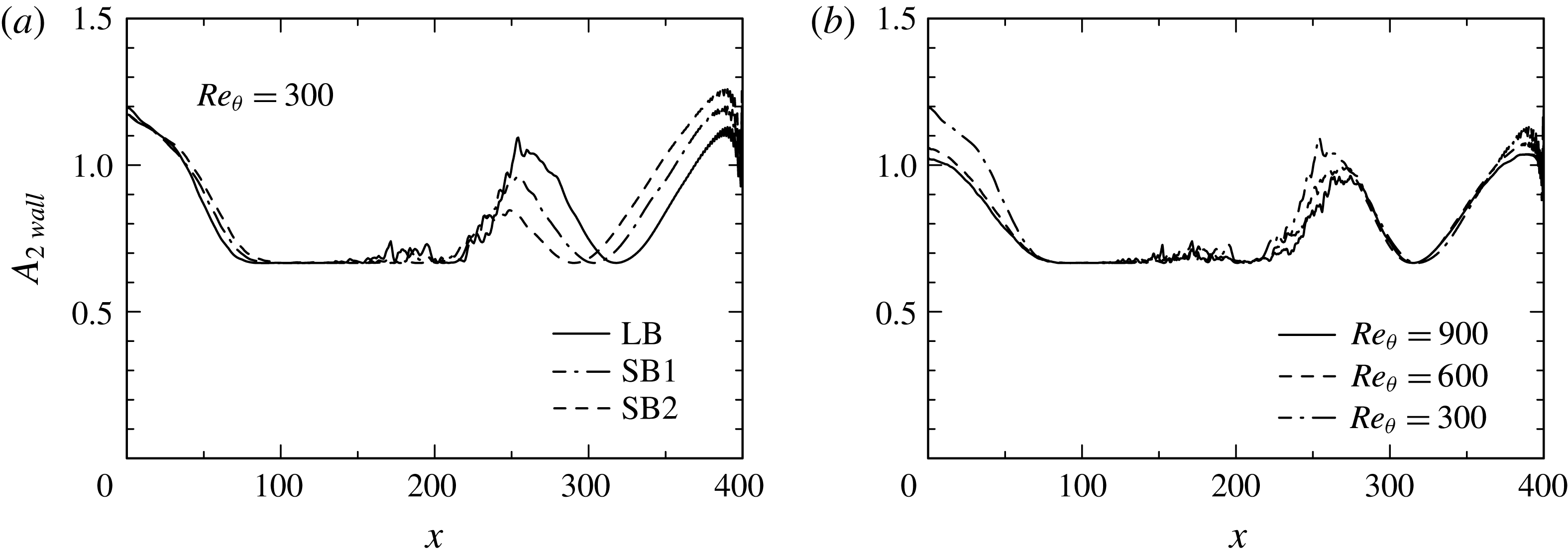
Distributions of
 $A_{2}$
at the wall: (a)
 $A_{2}$
for
 $Re_{\unicode[STIX]{x1D703}}=300$
obtained with three different magnitudes of
 $V_{top}$
; (b)
 $A_{2}$
for
 $Re_{\unicode[STIX]{x1D703}}=300$
,
 $600$
and
 $900$
obtained with the largest
 $V_{top}$
(LB).

In the reattached region, there is weak development of near-wall turbulence and thus a large anisotropy of
 $\overline{u_{i}u_{j}}$
. Figure 17 illustrates a wall value of the second invariant of anisotropy tensor
 $$\begin{eqnarray}\displaystyle A_{2}=a_{ij}a_{ij}, & & \displaystyle\end{eqnarray}$$
where
 $$\begin{eqnarray}\displaystyle a_{ij}\equiv \frac{\overline{u_{i}u_{j}}}{k}-\frac{2}{3}\unicode[STIX]{x1D6FF}_{ij}. & & \displaystyle\end{eqnarray}$$
Isotropy is obtained when
 $A_{2}=0$
. Note that the wall value of
 $A_{2}$
has been obtained with the data at the first grid point. Unlike in the APG and separated regions (see also Krogstad & Skåre (Reference Krogstad and Skåre1995) who noted that the anisotropy is strongly reduced near the surface of an APG turbulent boundary layer), a large magnitude of
 $A_{2}$
appears after reattachment. The latter magnitude increases with the magnitude of
 $V_{top}$
due to the increased mean flow acceleration. This has an important implication on turbulence modelling that the near-wall normal-stress anisotropy needs to be taken into account (e.g.
 $v^{2}-f$
model by Durbin (Reference Durbin1991)) when predicting a pressure-induced turbulent separation bubble.
3.4 Frequency spectra of
$p_{w}$

Here, we examine frequency spectra of
 $p_{w}$
for
 $Re_{\unicode[STIX]{x1D703}}=300$
and
 $900$
to examine how the scaling laws with
 $\unicode[STIX]{x1D70C}\overline{vv}_{max}$
and
 $-\unicode[STIX]{x1D70C}\overline{uv}_{max}$
hold at low, intermediate and high frequencies. The frequency spectra are defined such that
 $$\begin{eqnarray}\displaystyle \overline{pp}=2\int _{0}^{\infty }\unicode[STIX]{x1D719}(\unicode[STIX]{x1D714})\text{d}\unicode[STIX]{x1D714}=2\int _{0}^{\infty }\unicode[STIX]{x1D714}\unicode[STIX]{x1D719}(\unicode[STIX]{x1D714})\text{d}(\log \unicode[STIX]{x1D714}), & & \displaystyle\end{eqnarray}$$
which are obtained with the same methodology as in Choi & Moin (Reference Choi and Moin1990) and Na & Moin (Reference Na and Moin1998b
). For
 $Re_{\unicode[STIX]{x1D703}}=300$
, the 19 200 time consecutive instantaneous
 $p_{w}$
(i.e.
 $TU_{0}/\unicode[STIX]{x1D703}_{0}=0\sim 5280$
) have been used at a time interval of
 $\unicode[STIX]{x0394}tU_{0}/\unicode[STIX]{x1D703}_{0}=0.275$
. The total sampling number of 19 200 is divided into 8 overlapping parts (50 % overlap) with 3840 frequency modes (
 $0<\unicode[STIX]{x1D714}\unicode[STIX]{x1D703}_{0}/U_{0}<11.4$
). For
 $Re_{\unicode[STIX]{x1D703}}=900$
, the 34 560 time consecutive instantaneous
 $p_{w}$
(i.e.
 $TU_{0}/\unicode[STIX]{x1D703}_{0}=0\sim 3168$
) have been used at a time interval of
 $\unicode[STIX]{x0394}tU_{0}/\unicode[STIX]{x1D703}_{0}=0.275$
. The total sampling number of 34 560 is divided into 6 overlapping parts (50 % overlap) with 11 520 frequency modes (
 $0<\unicode[STIX]{x1D714}\unicode[STIX]{x1D703}_{0}/U_{0}<34.3$
).
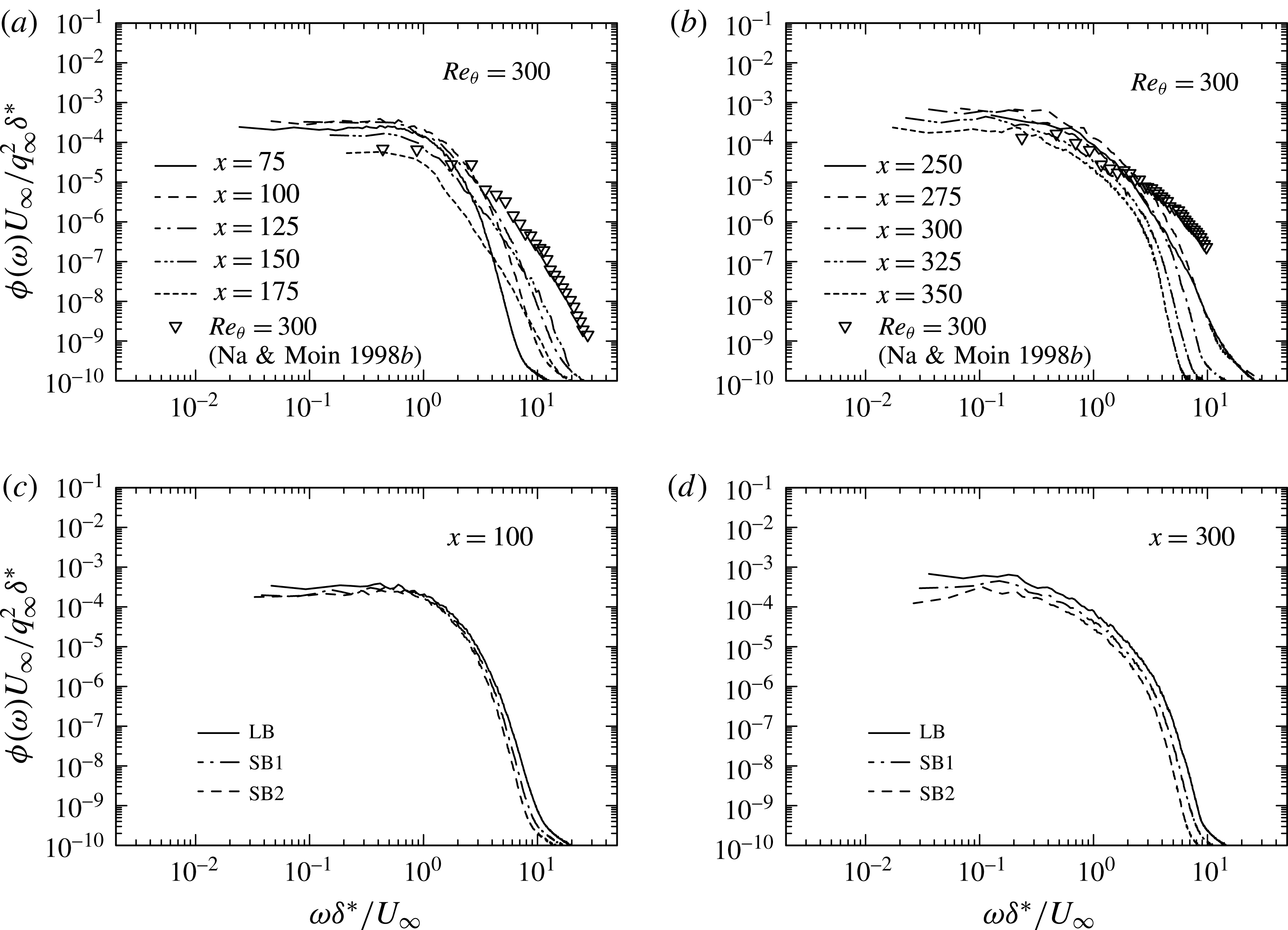
Figure 18 shows frequency spectra of
 $p_{w}$
normalized by the outer scaling
 $q_{\infty }^{2}\unicode[STIX]{x1D6FF}^{\ast }/U_{\infty }$
for
 $Re_{\unicode[STIX]{x1D703}}=300$
for the largest
 $V_{top}$
(LB) at several
 $x$
stations. In the APG and separated regions, the spectrum shows near plateau at low and intermediate frequencies, while it tends to show a
 $-11/3$
slope (the slope being close to that in free shear flows as discussed below) at high frequencies with moving downstream. The spectrum is essentially identical near separation independently of the magnitude of
 $V_{top}$
(see figure 18
c). This result collaborates with that of
 $p_{w\,rms}/q_{0}$
(see figure 8
a). In the reattached region, there is however no longer the plateau at low frequencies. Instead, the power decreases gradually towards high frequencies. In this region, there is a discernible effect of FPG, i.e. the power increases monotonically with increasing the magnitude of
 $V_{top}$
over the whole frequencies (see figure 18
d).
Frequency spectra of
 $p_{w}$
normalized by
 $q_{\infty }^{2}\unicode[STIX]{x1D6FF}^{\ast }/U_{\infty }$
for
 $Re_{\unicode[STIX]{x1D703}}=300$
: (a)
 $\unicode[STIX]{x1D719}(\unicode[STIX]{x1D714})U_{\infty }/q_{\infty }^{2}\unicode[STIX]{x1D6FF}^{\ast }$
in the APG and separated regions; (b)
 $\unicode[STIX]{x1D719}(\unicode[STIX]{x1D714})U_{\infty }/q_{\infty }^{2}\unicode[STIX]{x1D6FF}^{\ast }$
in the reattached region; (c)
 $\unicode[STIX]{x1D719}(\unicode[STIX]{x1D714})U_{\infty }/q_{\infty }^{2}\unicode[STIX]{x1D6FF}^{\ast }$
near separation (
 $x=100$
); (d)
 $\unicode[STIX]{x1D719}(\unicode[STIX]{x1D714})U_{\infty }/q_{\infty }^{2}\unicode[STIX]{x1D6FF}^{\ast }$
after reattachment (
 $x=300$
). The data obtained with the largest
 $V_{top}$
(LB) are plotted in (a) and (b), whereas those obtained with three different magnitudes of
 $V_{top}$
(i.e. SB1, SB2, LB) are plotted in (c) and (d).

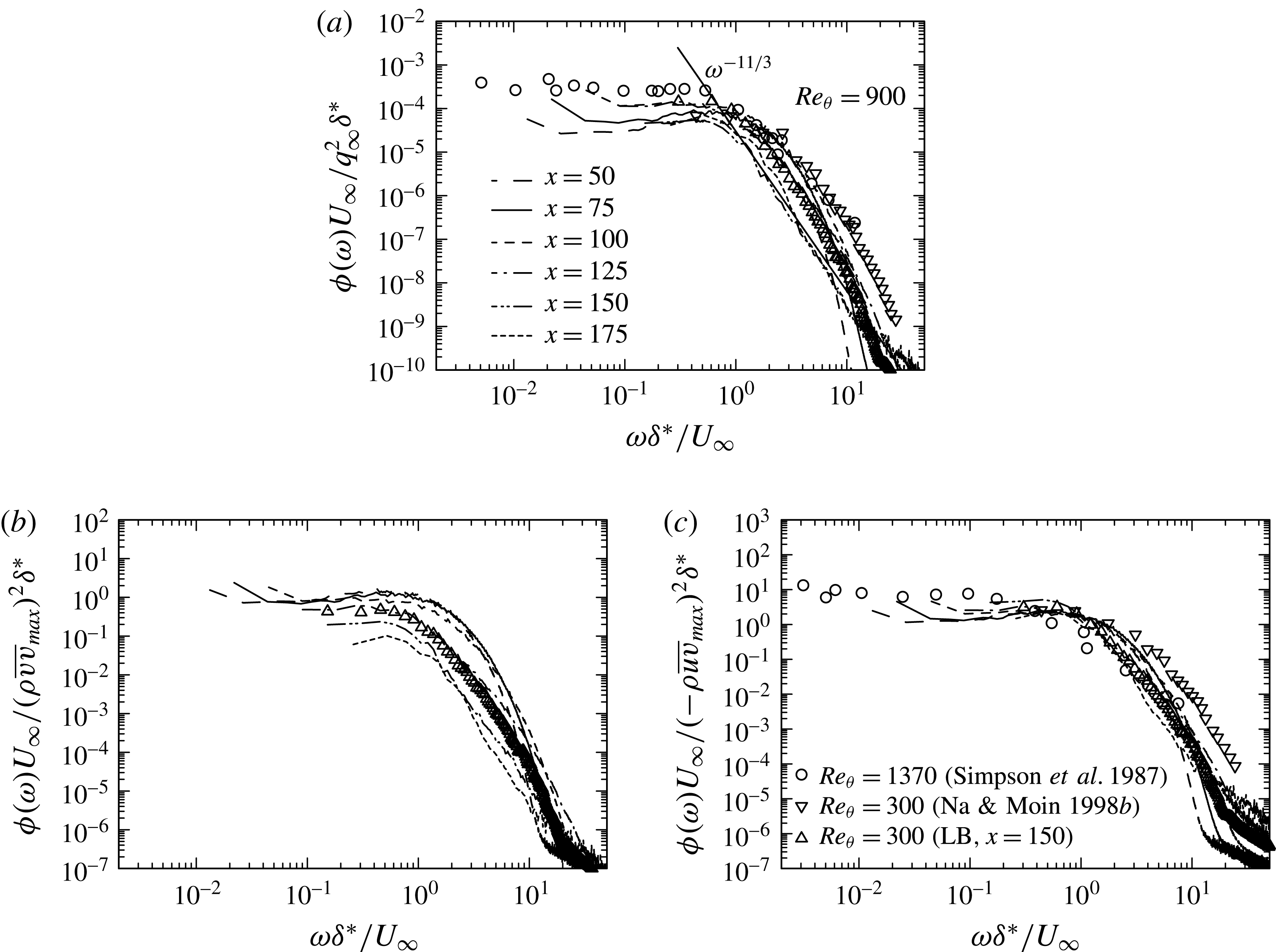
Frequency spectra of
 $p_{w}$
for
 $Re_{\unicode[STIX]{x1D703}}=900$
with three different types of normalization in the APG and separated regions: (a)
 $\unicode[STIX]{x1D719}(\unicode[STIX]{x1D714})$
normalized by
 $q_{\infty }^{2}\unicode[STIX]{x1D6FF}^{\ast }/U_{\infty }$
; (b)
 $\unicode[STIX]{x1D719}(\unicode[STIX]{x1D714})$
normalized by
 $(\unicode[STIX]{x1D70C}\overline{vv}_{\max })^{2}\unicode[STIX]{x1D6FF}^{\ast }/U_{\infty }$
; (c)
 $\unicode[STIX]{x1D719}(\unicode[STIX]{x1D714})$
normalized by
 $(-\unicode[STIX]{x1D70C}\overline{uv}_{\max })^{2}\unicode[STIX]{x1D6FF}^{\ast }/U_{\infty }$
. The data plotted in this figure have been obtained with the largest
 $V_{top}$
(LB).

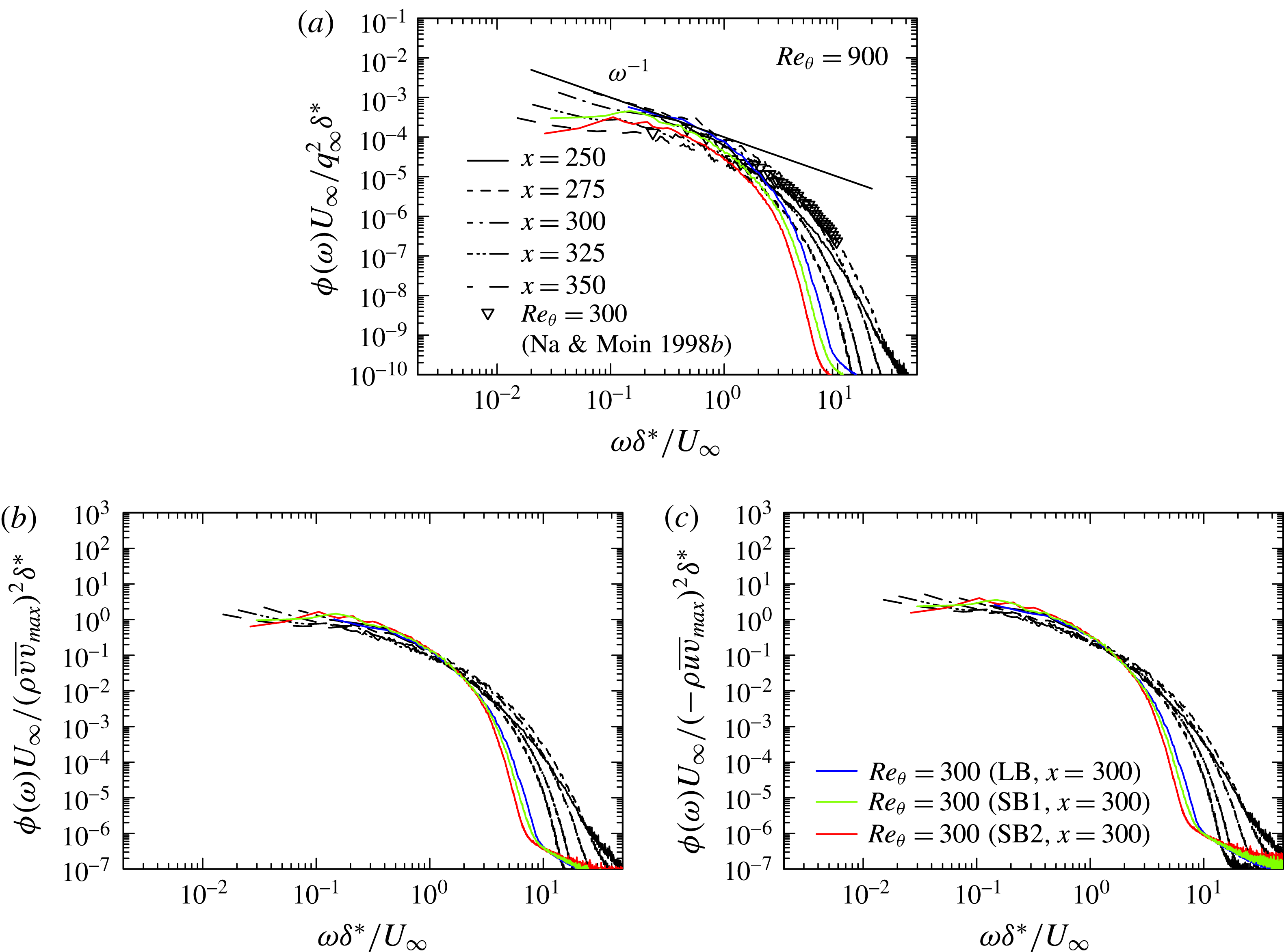
Frequency spectra of
 $p_{w}$
for
 $Re_{\unicode[STIX]{x1D703}}=900$
with three different types of normalization in the reattached and recovery regions: (a)
 $\unicode[STIX]{x1D719}(\unicode[STIX]{x1D714})$
normalized by
 $q_{\infty }^{2}\unicode[STIX]{x1D6FF}^{\ast }/U_{\infty }$
; (b)
 $\unicode[STIX]{x1D719}(\unicode[STIX]{x1D714})$
normalized by
 $(\unicode[STIX]{x1D70C}\overline{vv}_{max})^{2}\unicode[STIX]{x1D6FF}^{\ast }/U_{\infty }$
; (c)
 $\unicode[STIX]{x1D719}(\unicode[STIX]{x1D714})$
normalized by
 $(-\unicode[STIX]{x1D70C}\overline{uv}_{max})^{2}\unicode[STIX]{x1D6FF}^{\ast }/U_{\infty }$
. The data plotted in this figure have been obtained with the largest
 $V_{top}$
(LB). In (b) and (c), also plotted are the data for
 $Re_{\unicode[STIX]{x1D703}}=300$
at
 $x=300$
obtained with three different magnitudes of
 $V_{top}$
(i.e. SB1, SB2, LB) to discuss the scaling law of the spectra.

Figure 19 shows the frequency spectra for
 $Re_{\unicode[STIX]{x1D703}}=900$
in the APG and separated regions, as compared with those of Na & Moin (Reference Na and Moin1998b
) for
 $Re_{\unicode[STIX]{x1D703}}=300$
and Simpson et al. (Reference Simpson, Ghodbane and Mcgrath1987) for
 $Re_{\unicode[STIX]{x1D703}}=1380$
. The present data for
 $Re_{\unicode[STIX]{x1D703}}=300$
with three different magnitudes of
 $V_{top}$
are also included. Three types of normalization are used on the basis of scaling laws established for
 $p_{w\,rms}$
, viz. normalization with
 $q_{\infty }^{2}\unicode[STIX]{x1D6FF}^{\ast }/U_{\infty }$
,
 $(\unicode[STIX]{x1D70C}\overline{vv}_{max})^{2}\unicode[STIX]{x1D6FF}^{\ast }/U_{\infty }$
and
 $(-\unicode[STIX]{x1D70C}\overline{uv}_{max})^{2}\unicode[STIX]{x1D6FF}^{\ast }/U_{\infty }$
. Clearly, the best collapse of the spectra is obtained when normalization is made with the use of
 $-\unicode[STIX]{x1D70C}\overline{uv}_{max}$
, consistent with near plateau of
 $p_{w\,rms}/-\unicode[STIX]{x1D70C}\overline{uv}_{max}$
in the APG and separated regions (see figure 19). In the latter regions, the spectrum scales well on
 $-\unicode[STIX]{x1D70C}\overline{uv}_{max}$
at low frequencies. In particular, near plateau is observed at low frequencies below the frequency range of
 $\unicode[STIX]{x1D714}\unicode[STIX]{x1D6FF}^{\ast }/U_{\infty }\approx 1$
instead of the
 $\unicode[STIX]{x1D714}^{-0.7}$
behaviour (Simpson et al.
Reference Simpson, Ghodbane and Mcgrath1987). On the other hand, the power decreases gradually at intermediate and high frequencies as moving downstream. In the separated region, the spectral shape is close to that in the mixing layer (Jones et al.
Reference Jones, Adrian, Nithianandan and Planchon1979) due to effects of large
 $\unicode[STIX]{x2202}\overline{U}/\unicode[STIX]{x2202}y$
in the separated shear layer (see the
 $\unicode[STIX]{x1D714}^{-11/3}$
spectral behaviour at
 $x=150$
). In this context, the
 $\unicode[STIX]{x1D714}^{-11/3}$
spectral behaviour was obtained theoretically by George, Beuther & Arndt (Reference George, Beuther and Arndt1984) who considered turbulence and mean shear interaction in free shear flows. Kim (Reference Kim1989) also observed the
 $\unicode[STIX]{x1D714}^{-11/3}$
spectral behaviour for the rapid pressure, viz. pressure fluctuations obtained by solving the Poisson equation for turbulence and mean shear interaction, in a turbulent channel flow at the centreline.
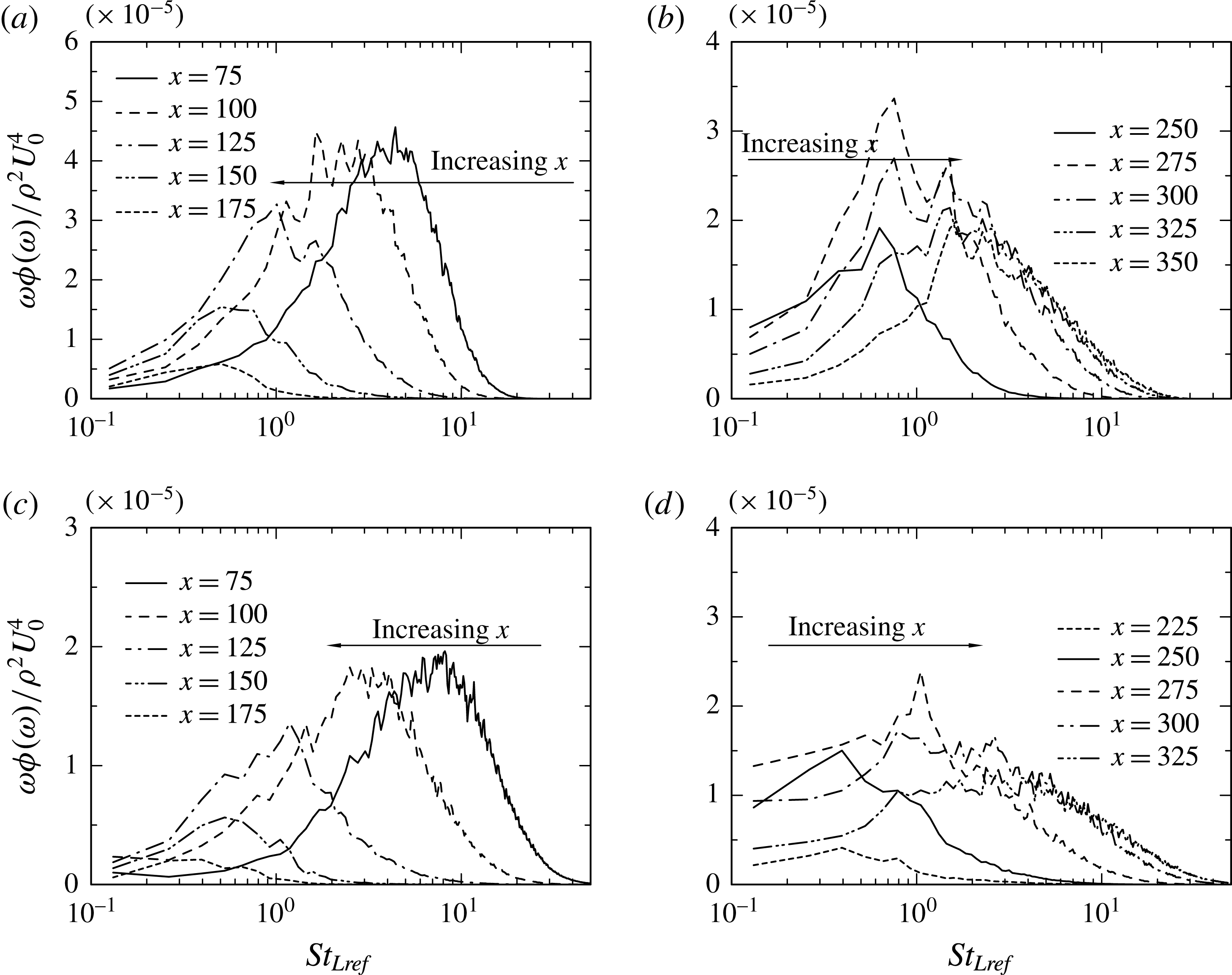
Pre-multiplied frequency spectra of
 $p_{w}$
normalized by
 $\unicode[STIX]{x1D70C}^{2}U_{0}^{4}$
for
 $Re_{\unicode[STIX]{x1D703}}=300$
((a), (b)) and
 $900$
((c), (d)): (a), (c)
 $\unicode[STIX]{x1D714}\unicode[STIX]{x1D719}(\unicode[STIX]{x1D714})/\unicode[STIX]{x1D70C}^{2}U_{0}^{4}$
in the APG and separated regions; (b), (d)
 $\unicode[STIX]{x1D714}\unicode[STIX]{x1D719}(\unicode[STIX]{x1D714})/\unicode[STIX]{x1D70C}^{2}U_{0}^{4}$
in the reattached and recovery regions. The data plotted in this figure have been obtained with the largest
 $V_{top}$
(LB).

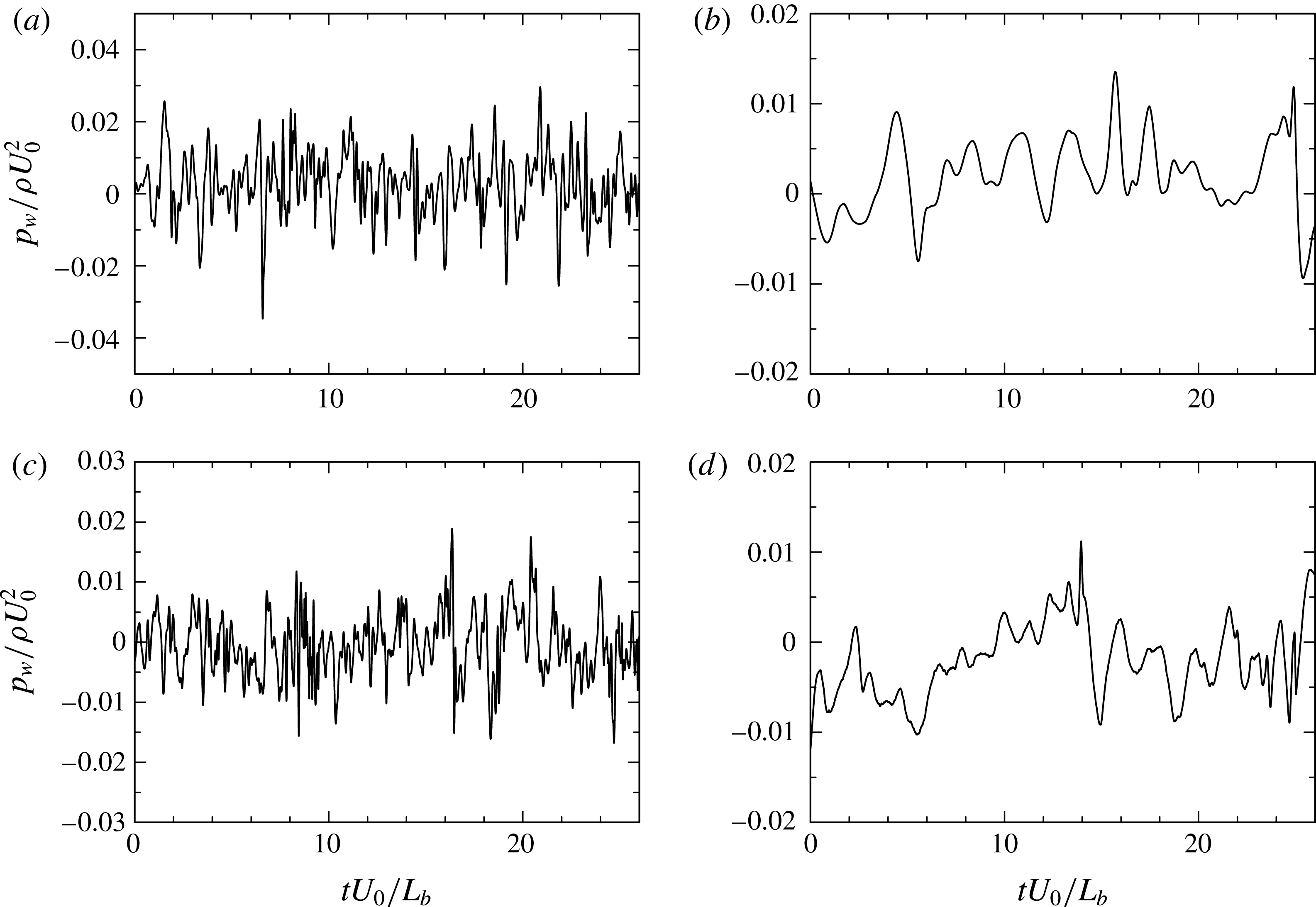
Time variation of instantaneous
 $p_{w}/\unicode[STIX]{x1D70C}U_{0}^{2}$
for
 $Re_{\unicode[STIX]{x1D703}}=300$
((a), (b)) and
 $900$
((c), (d)): (a), (c)
 $p_{w}/\unicode[STIX]{x1D70C}U_{0}^{2}$
near separation; (b), (d)
 $p_{w}/\unicode[STIX]{x1D70C}U_{0}^{2}$
near reattachment. The data plotted in this figure have been obtained with the largest
 $V_{top}$
(LB).

In the reattached region (figure 20), the low frequency behaviour becomes more pronounced than in the separated region (figure 19) since large-scale rollers generated in the separated shear layer propagate downstream and then impinge on the wall (see § 3.5). There is no longer the
 $\unicode[STIX]{x1D714}^{-11/3}$
behaviour at intermediate and high frequencies. Rather, the spectral slope is close to
 $-1$
at intermediate frequencies. It has been argued in a ZPG turbulent boundary layer that the contribution of eddies in the logarithmic region to
 $p_{w}$
leads to a
 $-1$
slope in the spectrum (see Bradshaw Reference Bradshaw1967; Panton & Lineberger Reference Panton and Lineberger1974; Blake Reference Blake1986; Choi & Moin Reference Choi and Moin1990). Tsuji et al. (Reference Tsuji, Fransson, Alfredsson and Johansson2007) recently reported that a
 $-0.7$
spectral slope is obtained in their measurements of a ZPG turbulent boundary layer up to
 $Re_{\unicode[STIX]{x1D703}}=2\times 10^{4}$
. They attributed the departure from the
 $-1$
slope to the limited Reynolds number and noted that an overlap region with the
 $-1$
slope is beyond the reach of laboratory measurements. In the reattached region of the present flow, there is also a discernible departure from the
 $-1$
slope, which is essentially associated with the slow recovery to the zero-pressure-gradient state in this region. When the spectra are normalized by either
 $-\overline{uv}_{max}$
or
 $\overline{vv}_{max}$
(figures 20
b and 20
c), reasonable collapse is obtained at several downstream stations at low and intermediate frequencies. This supports the present scaling laws established for
 $p_{w\,rms}$
near reattachment (see figure 13).
We also discuss the most energetic frequency of
 $p_{w}$
with the use of the pre-multiplied spectra
 $\unicode[STIX]{x1D714}\unicode[STIX]{x1D719}(\unicode[STIX]{x1D714})$
(i.e. the last term of (3.7)). The peak frequency of the pre-multiplied spectrum corresponds to the most energetic time scale contributing to the mean square value. In this context, Mabey (Reference Mabey1972) examined peak frequencies of the pre-multiplied spectra near reattachment for several types of the bubble. He reported that the Strouhal number for the spectral peak is most likely scaled on
 $L_{b}$
(the bubble length) and
 $U_{\infty }$
and that the resulting
 $St_{L}(\equiv fL_{b}/U_{\infty })$
is in the range 0.5–0.8 (
 $f(\equiv \unicode[STIX]{x1D714}/2\unicode[STIX]{x03C0})$
denotes the frequency). In the present flow, Weiss et al. (Reference Weiss, Mohammed-Taifour and Schwaab2015) recently pointed out the presence of two peaks in the pre-multiplied spectra for
 $Re_{\unicode[STIX]{x1D703}}=5000$
, viz.
 $St_{L\,ref}=0.01$
and
 $0.35$
. They demonstrated that the very low frequency mode
 $St_{L\,ref}=0.01$
, identical with that observed in the shock-turbulence boundary layer interaction (e.g. Touber & Sandham (Reference Touber and Sandham2009)), is responsible for a global oscillation of the bubble (i.e. contraction/expansion of the breathing motion), while the
 $St_{L\,ref}=0.35$
mode is due to the vortex shedding from the separated shear layer.
Figure 21 shows the pre-multiplied frequency spectra of
 $p_{w}$
at several streamwise stations for
 $Re_{\unicode[STIX]{x1D703}}=300$
and
 $900$
. Note that very low frequency mode
 $St_{L\,ref}=0.01$
reported by Weiss et al. (Reference Weiss, Mohammed-Taifour and Schwaab2015) is not resolved in the present frequency spectra. This figure highlights that the most energetic frequencies reside at lower frequencies in the bubble (i.e.
 $St_{L\,ref}=0.3\sim 1$
) than in the APG and reattached regions. In the separated region (
 $x\approx 150$
), a spectral peak of
 $p_{w}$
appears at
 $St_{L\,ref}=0.3\sim 0.4$
for both
 $Re_{\unicode[STIX]{x1D703}}=300$
and
 $900$
. In the reattached region (
 $x\approx 250$
), the low frequency behaviour becomes more prominent with increasing
 $Re_{\unicode[STIX]{x1D703}}$
. Time history of instantaneous
 $p_{w}$
supports this finding (see figure 22). For
 $Re_{\unicode[STIX]{x1D703}}=900$
, a spectral peak is also obtained at
 $St_{L\,ref}=0.3\sim 0.4$
near reattachment, which is the same
 $St_{L\,ref}$
as in the separated region. This Strouhal number agrees well with that obtained by Weiss et al. (Reference Weiss, Mohammed-Taifour and Schwaab2015) for
 $Re_{\unicode[STIX]{x1D703}}=5000$
, which is physically associated with the vortex shedding from the separated shear layer (see figures 24
c and 24
d where spanwise roller structures of low pressure regions become more pronounced with increasing
 $Re_{\unicode[STIX]{x1D703}}$
). The Strouhal number of
 $St_{L\,ref}=0.3\sim 0.4$
corresponds to
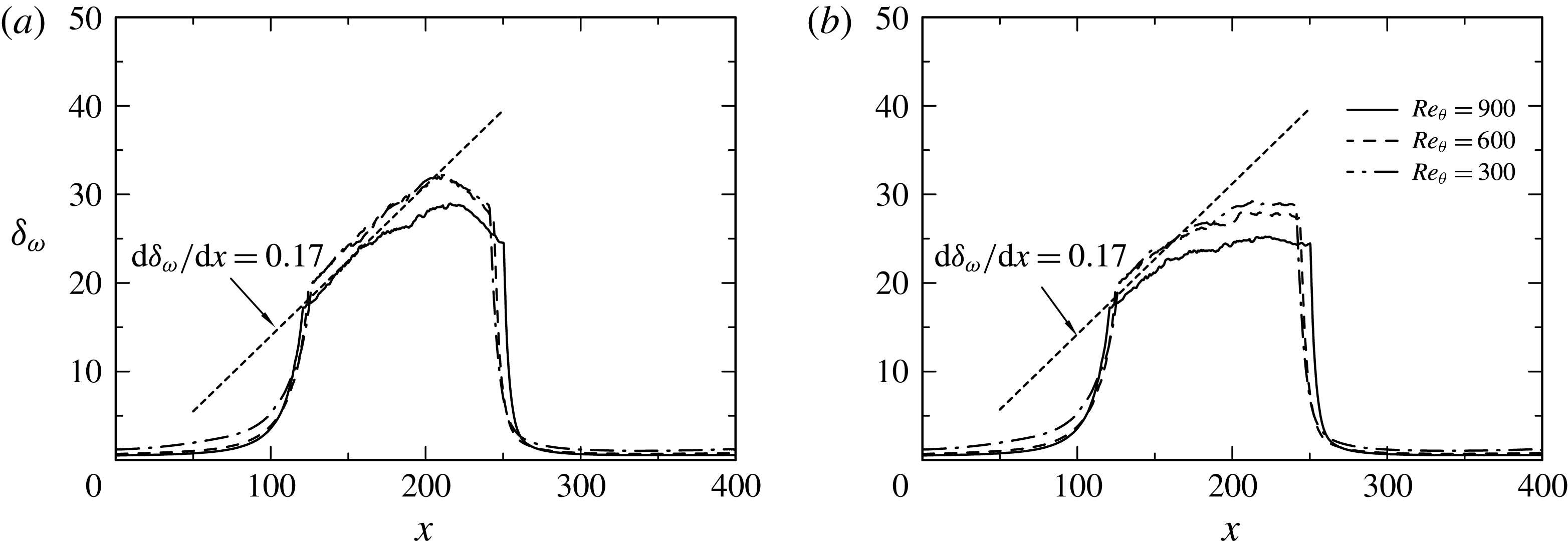
 $St_{\unicode[STIX]{x1D6FF}_{\unicode[STIX]{x1D714}}}\equiv f\unicode[STIX]{x1D6FF}_{\unicode[STIX]{x1D714}}/U_{sl}=0.2$
in the mixing layer (
 $St_{\unicode[STIX]{x1D6FF}_{\unicode[STIX]{x1D714}}}$
denotes the Strouhal number based on the vorticity thickness
 $\unicode[STIX]{x1D6FF}_{\unicode[STIX]{x1D714}}$
(defined in (3.8)) and the shear layer velocity
 $U_{sl}(=U_{\infty }/2)$
). In this context, Driver, Seegmiller & Marvin (Reference Driver, Seegmiller and Marvin1987) also reported the dominant frequency of
 $St_{\unicode[STIX]{x1D6FF}_{\unicode[STIX]{x1D714}}}=0.2$
in their backward-facing step and noted close relationship with characteristic frequency of spanwise vortical structures in free shear layers.
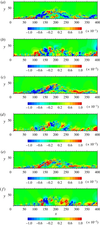
Contours of instantaneous
 $u/U_{0}$
and
 $p/\unicode[STIX]{x1D70C}U_{0}^{2}$
in the
 $x{-}y$
plane for
 $Re_{\unicode[STIX]{x1D703}}=300$
((a), (b)),
 $600$
((c), (d)) and
 $900$
((e), (f)): (a), (c), (e)
 $u/U_{0}$
; (b), (d), (f)
 $p/\unicode[STIX]{x1D70C}U_{0}^{2}$
. The data plotted in this figure have been obtained with the largest
 $V_{top}$
(LB).

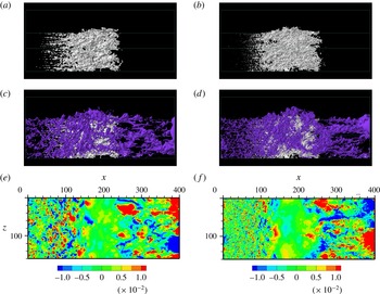
Isosurfaces of instantaneous
 $p$
together with those of
 $U=0$
for
 $Re_{\unicode[STIX]{x1D703}}=300$
and
 $900$
as compared with contours of
 $p_{w}$
: (a) white,
 $U=0$
(
 $Re_{\unicode[STIX]{x1D703}}=300$
); (b) white,
 $U=0$
(
 $Re_{\unicode[STIX]{x1D703}}=900$
); (c) blue,
 $p<-0.008$
and white,
 $U=0$
(
 $Re_{\unicode[STIX]{x1D703}}=300$
); (d) blue,
 $p<-0.008$
and white,
 $U=0$
(
 $Re_{\unicode[STIX]{x1D703}}=900$
); (e) contours of
 $p_{w}$
(
 $Re_{\unicode[STIX]{x1D703}}=300$
); (f) contours of
 $p_{w}$
(
 $Re_{\unicode[STIX]{x1D703}}=900$
). The visualization domain size shown here is the whole computational domain. The fluid flows from left to right. The data plotted in this figure have been obtained with the largest
 $V_{top}$
(LB).

3.5 Structures of
$p_{w}$

In this subsection, we investigate structures of pressure fluctuations above the wall and the relationship with wall-pressure fluctuations. Particular attention is given to the largest
 $V_{top}$
case (LB), i.e. a large separation bubble. Contours of instantaneous pressure fluctuations
 $p/\unicode[STIX]{x1D70C}U_{0}^{2}$
in the
 $x{-}y$
plane are shown in figure 23 for
 $Re_{\unicode[STIX]{x1D703}}=300$
,
 $600$
and
 $900$
together with those of instantaneous streamwise velocity fluctuations
 $u/U_{0}$
. After separation, turbulence structures in an APG boundary layer are lifted above the bubble, where positive and negative pressure fluctuations appear alternatively along the separated shear layer as a result of the roll-up process. They then turn around the bubble and subsequently impinge on the wall. Indeed, this impingement yields large wall-pressure fluctuations in the reattached region (see figures 24
e and 24
f). As for the
 $Re$
dependence, turbulence structures become more energetic in the APG and separated regions at lower
 $Re_{\unicode[STIX]{x1D703}}$
when normalization is made with the use of the inlet reference velocity
 $U_{0}$
(see figure 23) since effects of an incoming boundary layer are dominated over these regions (see the discussion in § 3.2). Above the bubble, large scales are dominated at large
 $Re_{\unicode[STIX]{x1D703}}$
. In particular, large-scale negative
 $p$
structures tend to appear with increasing
 $Re_{\unicode[STIX]{x1D703}}$
, which are large-scale spanwise rollers as discussed below (note that large and small scales are hardly distinguished at
 $Re_{\unicode[STIX]{x1D703}}=300$
due to low
 $Re$
effects).
Figure 24(a–d) shows isosurfaces of negative
 $p$
for
 $Re_{\unicode[STIX]{x1D703}}=300$
and
 $900$
together with those of
 $U=0$
(the latter illustrating a shape of the separation bubble). As noted by Manhart & Friedrich (Reference Manhart and Friedrich2002), a highly irregular shape of the bubble appears in the isosurfaces of
 $U=0$
where detachment tends to occur intermittently (Simpson et al.
Reference Simpson, Chew and Shivaprasad1981) in the region associated with near-wall streaks (see also Na & Moin Reference Na and Moin1998a
). The separation point is rather difficult to be defined as a line. As for the negative
 $p$
regions, hairpin-like spanwise structures tend to emerge as the separation point is approached. The spanwise structures become increasingly larger along the separated shear layer and form large-scale spanwise rollers above the bubble. The latter structures are similar to two-dimensional rollers observed in turbulent mixing layers (see Rogers & Moser Reference Rogers and Moser1994). Figures 24(c) and 24(d) highlight that the large-scale spanwise rollers appear more clearly with increasing Reynolds number, whilst the number of small scales increases with
 $Re_{\unicode[STIX]{x1D703}}$
inside large scales. Troutt, Scheelke & Norman (Reference Troutt, Scheelke and Norman1984) also observed large spanwise vortices in their measurement of a backward facing step flow.
Distributions of the vorticity thickness
 $\unicode[STIX]{x1D6FF}_{\unicode[STIX]{x1D714}}$
for
 $Re_{\unicode[STIX]{x1D703}}=300$
,
 $600$
and
 $900$
: (a)
 $\unicode[STIX]{x1D6FF}_{\unicode[STIX]{x1D714}}$
obtained with the full velocity difference; (b)
 $\unicode[STIX]{x1D6FF}_{\unicode[STIX]{x1D714}}$
obtained with
 $U_{min}=0$
. The data plotted in this figure have been obtained with the largest
 $V_{top}$
(LB).

Contours of
 $\overline{U}/U_{0}$
for
 $Re_{\unicode[STIX]{x1D703}}=900$
: (a)
 $\overline{U}/U_{0}$
with the dividing streamline (— ⋅ —), locations of
 $\overline{U}_{max}$
(——),
 $\overline{U}_{min}$
(– – –), and the centre of the separated shear layer
 $\overline{uu}_{max}$
(
 $\cdots \cdots$
); (b) a magnified view of the vector field in the recirculation zone with the dividing streamline (— ⋅ —) and location of
 $\overline{U}_{min}$
(– – –). Note that figure 10(b) is replotted in (a) to highlight locations of
 $\overline{U}_{max}$
and
 $\overline{U}_{min}$
, whereas it is in (b) to highlight the large recirculation region of the bubble. In (a), solid and dashed lines denote positive and negative streamlines, respectively.

Isosurfaces of instantaneous
 $p$
,
 $u$
and
 $Q$
for
 $Re_{\unicode[STIX]{x1D703}}=900$
: (a) white,
 $p<-0.008$
; (b) white,
 $Q>0.01$
; (c) red,
 $u>0.15$
; blue,
 $u<-0.15$
. The visualization domain size shown here is the whole computational domain. The fluid flows from bottom left to top right. The data plotted in this figure have been obtained with the largest
 $V_{top}$
(LB).

To examine the degree of similarity to the mixing layer, figure 25 shows distributions of the vorticity thickness
 $\unicode[STIX]{x1D6FF}_{\unicode[STIX]{x1D714}}$
defined such that
 $$\begin{eqnarray}\displaystyle \unicode[STIX]{x1D6FF}_{\unicode[STIX]{x1D714}}\equiv (\overline{U}_{max}-\overline{U}_{min})/(\unicode[STIX]{x2202}\overline{U}/\unicode[STIX]{x2202}y)_{max}, & & \displaystyle\end{eqnarray}$$
where
 $\overline{U}_{max}$
and
 $\overline{U}_{min}$
denote the maximum and minimum values of
 $\overline{U}$
(see figure 26 where locations of
 $\overline{U}_{min}$
and
 $\overline{U}_{max}$
for
 $Re_{\unicode[STIX]{x1D703}}=900$
are shown). Note that while Troutt et al. (Reference Troutt, Scheelke and Norman1984) used
 $\overline{U}_{min}=0$
in a backward facing step, the present study examines a difference between
 $\unicode[STIX]{x1D6FF}_{\unicode[STIX]{x1D714}}$
obtained with the use of both actual minimum velocity
 $\overline{U}_{min}$
and that with
 $\overline{U}_{min}=0$
(see figure 25). Note also that the present simulation for the largest
 $V_{top}$
case (LB) exhibits a large recirculation region as in Patrick (Reference Patrick1987), Na & Moin (Reference Na and Moin1998b
) and Mohammed-Taifour & Weiss (Reference Mohammed-Taifour and Weiss2016) (see figure 26
b where a recirculation region is illustrated with mean velocity vector). It turns out that in the separated region (
 $120<x<210$
), the full velocity difference (viz.
 $\unicode[STIX]{x0394}U\equiv \overline{U}_{max}-\overline{U}_{min}$
) yields a slightly closer similarity to free shear flows than that obtained with
 $\overline{U}_{min}=0$
. This is consistent with the finding of Abe et al. (Reference Abe, Mizobuchi, Matsuo and Spalart2012) that the maximum values of
 $\overline{uu}$
,
 $\overline{vv}$
and
 $\overline{ww}$
normalized by the full velocity difference
 $\unicode[STIX]{x0394}U$
agree reasonably with those in the mixing layer. Figure 25 demonstrates that the present value of
 $d\unicode[STIX]{x1D6FF}_{\unicode[STIX]{x1D714}}/dx$
is close to 0.17 in the separated shear layer. The latter value agrees well with that of Brown & Roshko (Reference Brown and Roshko1974) in turbulent mixing layers. The present results underline that the large-scale spanwise
 $p$
structures observed in figures 24(c) and 24(d) are essentially associated with those in the mixing layer. The absence of braid structures (i.e. streamwise elongated structures between the rollers) seems to be due to the mean flow deceleration (i.e. the decrease of mean normal stress). It is also observed in figures 24(c) and 24(d) (see also figure 27
a) that large-scale spanwise rollers become more prominent with increasing
 $Re_{\unicode[STIX]{x1D703}}$
and propagate into the reattached region. At the reattachment, there is significant impingement of large-scale rollers. This impingement provides a large amount of backflow inside the bubble (see figure 26
b) where turbulence intensity is small (see figure 23). The resulting backflow subsequently interacts with vortical structures in the separated shear layer. There is thus close relationship between the backflow and vortex shedding mode in the present flow, which is most likely associated with the present finding on
 $\unicode[STIX]{x1D6FF}_{\unicode[STIX]{x1D714}}$
that (3.8) with the full velocity difference leads to a better similarity to free shear flows. The large-scale vortex shedding is intrinsically associated with the most energetic frequency of
 $p_{w}$
in the reattached region (i.e.
 $St_{L\,ref}=0.3\sim 0.4$
, or equivalently,
 $St_{\unicode[STIX]{x1D6FF}_{\unicode[STIX]{x1D714}}}=0.2$
). On the other hand, the separation bubble also involves a global oscillation (i.e. contraction/expansion of the bubble) (see Na & Moin Reference Na and Moin1998a
; Weiss et al.
Reference Weiss, Mohammed-Taifour and Schwaab2015; Mohammed-Taifour & Weiss Reference Mohammed-Taifour and Weiss2016). This global unsteady motion is however beyond the scope of the present study, which will be pursued in a future work.
After the top of the separation bubble, large-scale spanwise rollers propagate downstream by FPG and subsequently impinge on the wall. In the reattached region, convection is dominated so that the shear layer involves mean flow acceleration, i.e.
 $\unicode[STIX]{x2202}\overline{U}/\unicode[STIX]{x2202}x>0$
(or equivalently,
 $\unicode[STIX]{x2202}\overline{V}/\unicode[STIX]{x2202}y<0$
), near reattachment. This acceleration most likely yields streamwise elongated structures of negative
 $p$
between the rollers (see figures 24
c and 24
d). We also stress that the impingement of large-scale
 $p$
structures leads to a large magnitude of
 $p_{w}$
. Figures 24(e) and 24(f) show contours of instantaneous wall-pressure fluctuations for
 $Re_{\unicode[STIX]{x1D703}}=300$
and
 $900$
. Clearly, spanwise patterns are dominated near separation, whilst streamwise ones are after reattachment. The former patterns are associated with spanwise rollers of pressure fluctuations in the APG and separated regions, while the latter come from streamwise elongated negative
 $p$
structures in the reattached region. Interestingly, analogous streamwise elongated
 $p_{w}$
patterns are also observed in a region after reattachment of the cove separation bubble where a large recirculation region is created as in the present flow (see Imamura et al.
Reference Imamura, Enomoto, Yokokawa and Yamamoto2008). We also note that while we may not distinguish large and small scales for
 $Re_{\unicode[STIX]{x1D703}}=300$
due to the limited scale separation (figure 24
e), large scales are more dominated in the reattached region than in region near separation for
 $Re_{\unicode[STIX]{x1D703}}=900$
(figure 24
f). The latter is attributed to the increased amalgamation of spanwise roller structures as they propagate downstream.
Spanwise pre-multiplied wavenumber spectra of
 $u$
and
 $p$
,
 $k_{z}\unicode[STIX]{x1D719}_{uu}(k_{z})/U_{0}^{2}$
and
 $k_{z}\unicode[STIX]{x1D719}_{pp}(k_{z})/\unicode[STIX]{x1D70C}^{2}U_{0}^{4}$
, for
 $Re_{\unicode[STIX]{x1D703}}=300$
,
 $600$
and
 $900$
at
 $y/\unicode[STIX]{x1D703}_{0}=10$
: (a), (c)
 $k_{z}\unicode[STIX]{x1D719}_{uu}(k_{z})/U_{0}^{2}$
; (b), (d)
 $k_{z}\unicode[STIX]{x1D719}_{pp}(k_{z})/\unicode[STIX]{x1D70C}^{2}U_{0}^{4}$
. The
 $x$
locations examined are at
 $x/\unicode[STIX]{x1D703}_{0}=125$
((a), (b)) and
 $x/\unicode[STIX]{x1D703}_{0}=300$
((c), (d)). The data plotted in this figure have been obtained with the largest
 $V_{top}$
(LB). Also plotted for comparison are the spectra of a ZPG turbulent boundary layer for
 $Re_{\unicode[STIX]{x1D703}}=900$
.

Note that the similarity to the mixing layer in
 $u$
and
 $Q(\equiv -u_{i,j}u_{j,i}/2)$
is not as good as in
 $p$
(
 $Q$
denotes the second invariant of fluctuating velocity tensor). Isosurfaces of negative
 $p$
for
 $Re_{\unicode[STIX]{x1D703}}=900$
are illustrated in figure 27 together with those of positive
 $Q$
and
 $u$
. Unlike for negative
 $p$
, roller-like structures are not observed for
 $Q$
, but dense clustering structures appear in the separated shear layer (see also Abe et al.
Reference Abe, Mizobuchi, Matsuo and Spalart2012). In the latter region, large-scale positive and negative
 $u$
structures appear alternatively in the
 $z$
direction. The large-scale
 $u$
structures essentially come from those energised by the pressure gradient in the outer region of an APG boundary layer (see Lee & Sung Reference Lee and Sung2009; Monty, Harun & Marusic Reference Monty, Harun and Marusic2011). After separation, the later structures are lifted above the bubble and then become more energetic due to large
 $\unicode[STIX]{x2202}\overline{U}/\unicode[STIX]{x2202}y$
in the separated shear layer. As for negative
 $p$
, large-scale structures of positive and negative
 $u$
become more energetic in the reattached region than in the separated region (see figure 27
c). The latter behaviour may be quantified by examining spanwise wavenumber spectra of
 $u$
and
 $p$
defined such that
 $$\begin{eqnarray}\displaystyle \overline{uu}=\int _{0}^{\infty }\unicode[STIX]{x1D719}_{uu}(k_{z})\,\text{d}k_{z}=\int _{0}^{\infty }k_{z}\unicode[STIX]{x1D719}_{uu}(k_{z})\,\text{d}(\log k_{z}) & & \displaystyle\end{eqnarray}$$
and
 $$\begin{eqnarray}\displaystyle \overline{pp}=\int _{0}^{\infty }\unicode[STIX]{x1D719}_{pp}(k_{z})\,\text{d}k_{z}=\int _{0}^{\infty }k_{z}\unicode[STIX]{x1D719}_{pp}(k_{z})\,\text{d}(\log k_{z}), & & \displaystyle\end{eqnarray}$$
where
 $k_{z}$
is the spanwise wavenumber. Figure 28 shows the normalized spanwise pre-multiplied spectra of
 $u$
and
 $p$
in the separated and reattached regions. In the separated shear layer, the spectral peaks of
 $u$
appear at the spanwise wavelength of
 $\unicode[STIX]{x1D706}_{z}/\unicode[STIX]{x1D6FF}_{0}\approx 1.6$
(
 $\unicode[STIX]{x1D706}_{z}=2\unicode[STIX]{x03C0}/k_{z}$
), the value being twice as large as
 $\unicode[STIX]{x1D706}_{z}/\unicode[STIX]{x1D6FF}_{0}\approx 0.8$
(
 $\unicode[STIX]{x1D6FF}_{0}$
denotes the inlet boundary layer thickness) obtained in the outer part of a ZPG turbulent boundary layer. In the reattached region, the peaks move to larger wavelength of
 $\unicode[STIX]{x1D706}_{z}/\unicode[STIX]{x1D6FF}_{0}\approx 3.2$
. There is indeed an increase in the spanwise most energetic length scales for
 $u$
in the reattached region. The peak wavelengths correspond well to spanwise spacings between the negative
 $u$
structures (also those between the positive
 $u$
structures) shown in figure 28(c). A possible scenario of the spanwise scale increase is most likely the merging of adjacent structures. The large-scale structures observed for
 $u$
are essentially the phenomena affected by the shear layer in both separated and reattached regions. On the other hand, the spectral peak for
 $p$
tends to become less prominent in the separated shear layer with increasing
 $Re_{\unicode[STIX]{x1D703}}$
, consistent with the present finding that large-scale spanwise rollers become more dominated with increasing
 $Re_{\unicode[STIX]{x1D703}}$
. In this context, it is well recognized that the spanwise roller generated in the separated shear layer is a consequence of an inflectional hydrodynamic instability as in mixing layers (see Na & Moin Reference Na and Moin1998b
; Thacker et al.
Reference Thacker, Auburn, Leroy and Devinant2013). In the reattached region where the large-scale spanwise rollers of negative
 $p$
are broken down due to the impingement on the wall (see figures 24
c, 24
d and 27
a), the spectral peaks for
 $p$
appear at nearly the same wavelengths as for
 $u$
. In this region, negative
 $p$
regions are also closely associated with those of both negative
 $u$
and positive
 $Q$
. This behaviour is essentially associated with convective nature of a pressure-induced separation bubble near reattachment where the mean shear involves mean flow acceleration.
4 Conclusions
In the present study, we have examined DNS datasets of a pressure-induced turbulent separation bubble on a flat plate for
 $Re_{\unicode[STIX]{x1D703}}=300$
,
 $600$
and
 $900$
(Abe et al.
Reference Abe, Mizobuchi, Matsuo and Spalart2015). Particular attention is given to Reynolds-number dependence of
 $p_{w}$
. Possible scaling laws of the r.m.s. values and frequency spectra are also examined as compared with the existing DNS (Spalart & Coleman Reference Spalart and Coleman1997; Na & Moin Reference Na and Moin1998b
) and experiments (Simpson et al.
Reference Simpson, Ghodbane and Mcgrath1987; Weiss et al.
Reference Weiss, Mohammed-Taifour and Schwaab2015; Mohammed-Taifour & Weiss Reference Mohammed-Taifour and Weiss2016). The main conclusions are as follows.
-
(i) The r.m.s. value of wall-pressure fluctuations normalized by inlet dynamic pressure
$p_{w\,rms}/q_{0}$
is characterized by two local peaks. One peak is located near separation, which does not depend on APG, but weakly on
$Re_{\unicode[STIX]{x1D703}}$
. While the inactive motion contributes significantly to pressure fluctuations above the wall, turbulent shearing motion (i.e. the active motion) makes a substantial contribution to
$p_{w\,rms}/q_{0}$
in the APG and separated regions. The other peak is located after reattachment, which does not depend on
$Re_{\unicode[STIX]{x1D703}}$
, but on FPG. The latter affects the flow impingement on the wall and thus wall-pressure fluctuations in the reattached region. -
(ii) The similarity between
$p_{w\,rms}/q_{0}$
and
$-\overline{uv}_{max}/U_{0}^{2}$
is convincing in the APG and separated regions. In these regions, the magnitude of
$p_{w\,rms}/-\unicode[STIX]{x1D70C}\overline{uv}_{max}$
exhibits near plateau (i.e.
$2.5\sim 3$
), which underlines that vortical motion producing
$-\overline{uv}$
makes an important contribution to
$p_{w}$
. On the other hand,
$p_{w\,rms}$
collapses not only on
$-\unicode[STIX]{x1D70C}\overline{uv}_{max}$
but also on
$\unicode[STIX]{x1D70C}\overline{vv}_{max}$
in the reattached region.
$p_{w\,rms}/-\unicode[STIX]{x1D70C}\overline{uv}_{max}\approx 1.8$
and
$p_{w\,rms}/\unicode[STIX]{x1D70C}\overline{vv}_{max}\approx 1.2$
are attained unambiguously near reattachment independently of the Reynolds number and pressure gradient. The present value of
$p_{w\,rms}/\unicode[STIX]{x1D70C}\overline{vv}_{max}$
(1.2) is smaller than (1.35) obtained for step-induced separation by Ji & Wang (Reference Ji and Wang2012). The reason for this difference is intrinsically associated with convective nature of a pressure-induced separation bubble near reattachment where mean flow acceleration, i.e.
$\unicode[STIX]{x2202}\overline{U}/\unicode[STIX]{x2202}x>0$
(or equivalently,
$\unicode[STIX]{x2202}\overline{V}/\unicode[STIX]{x2202}y<0$
), is involved in the shear layer. This acceleration leads to delay of the
$p_{w\,rms}$
peak after reattachment and also normal Reynolds-stress anisotropy near the wall. -
(iii) The frequency spectra of
$p_{w}$
normalized by
$(-\unicode[STIX]{x1D70C}\overline{uv}_{max})^{2}\unicode[STIX]{x1D6FF}^{\ast }/U_{\infty }$
collapse reasonably at low frequencies in the APG and separated regions, which corroborates with the finding of Simpson et al. (Reference Simpson, Ghodbane and Mcgrath1987) and Na & Moin (Reference Na and Moin1998b
). The present results highlight that there is near plateau at low frequencies (viz.
$\unicode[STIX]{x1D714}\unicode[STIX]{x1D6FF}^{\ast }/U_{\infty }\leqslant 1$
) instead of the
$\unicode[STIX]{x1D714}^{-0.7}$
slope reported by Simpson et al. (Reference Simpson, Ghodbane and Mcgrath1987). In the separated region, the power decreases gradually at intermediate and high frequencies with moving downstream; the
$\unicode[STIX]{x1D714}^{-11/3}$
spectral behaviour is observed due to effects of large
$\unicode[STIX]{x2202}\overline{U}/\unicode[STIX]{x2202}y$
in the separated shear layer. In the reattached region, good collapse is obtained at low and intermediate frequencies when the spectra are non-dimensionalized by both
$(-\unicode[STIX]{x1D70C}\overline{uv}_{max})^{2}\unicode[STIX]{x1D6FF}^{\ast }/U_{\infty }$
and
$(\unicode[STIX]{x1D70C}\overline{vv}_{max})^{2}\unicode[STIX]{x1D6FF}^{\ast }/U_{\infty }$
. These results support the present scaling laws established for
$p_{w\,rms}$
. -
(iv) The most energetic frequencies of
$p_{w}$
reside at lower frequencies in the bubble than in the APG and reattached regions. In the reattached region, the low frequency behaviour becomes increasingly pronounced with
$Re_{\unicode[STIX]{x1D703}}$
. For
$Re_{\unicode[STIX]{x1D703}}=900$
, a low frequency peak is obtained in the pre-multiplied spectra (i.e. equation (3.7)) at the Strouhal number
$St_{L\,ref}=0.3\sim 0.4$
near reattachment. This peak Strouhal number agrees well with that obtained from the recent measurement of Weiss et al. (Reference Weiss, Mohammed-Taifour and Schwaab2015) (and also the subsequent work of Mohammed-Taifour & Weiss (Reference Mohammed-Taifour and Weiss2016)) for
$Re_{\unicode[STIX]{x1D703}}=5000$
, which also corresponds to
$St_{\unicode[STIX]{x1D6FF}_{\unicode[STIX]{x1D714}}}=0.2$
in the mixing layer. The present result underlines that the vortex shedding from the separated shear layer is essentially associated with a large magnitude of
$p_{w}$
in the reattached region. -
(v) After separation, turbulence structures in an APG boundary layer are lifted above the bubble where positive and negative pressure fluctuations appear alternatively along the separated shear layer as a consequence of the roll-up process. When the separation bubble is large, spanwise structures of low pressure fluctuations are dominated above the bubble, which are identical with those in free shear flows. The spanwise structures tend to form large-scale rollers with increasing
$Re_{\unicode[STIX]{x1D703}}$
, which convect downstream and subsequently impinge on the wall. This impingement affects
$p_{w}$
in the reattached region where the topology of
$p_{w}$
varies from spanwise patterns to streamwise ones owing to the presence of mean flow acceleration.















The present study underlines that there is a discernible difference in
 $p_{w}$
near reattachment between pressure-induced separation and step-induced one. In the present flow, convection is dominated in the reattached region where FPG affects the flow impingement on the wall and thus
 $p_{w}$
.
Acknowledgements
Computations performed on the JAXA (Japan Aerospace Exploration Agency) Supercomputer System are gratefully acknowledged. H.A. is grateful to Drs Y. Mizobuchi, Y. Matsuo and P. R. Spalart for their comments during the course of this work. H.A. also acknowledges discussions with Professors P. Moin, J. Eaton, G. Iaccarino, A. Yoshizawa, H. Kawamura and G. Kawahara.