1. Introduction
The space–time characteristics of large-scale structures in turbulent flows are of practical interest for engineering applications involving flow-induced noise and structural vibration (Williams & Kempton Reference Williams and Kempton1978; Blake Reference Blake2017). Predicting the space–time flow statistics typically resorts to scale-resolving simulations, such as large eddy simulation (LES) (He et al. Reference He, Wang and Lele2004, Reference He, Jin and Yang2017) and direct numerical simulation (DNS) (Choi & Moin Reference Choi and Moin1990). However, such methods require resolving most flow scales to capture interscale energy transfer, making them computationally prohibitive for flows with high Reynolds numbers due to significant scale separation. Therefore, it is highly demanding to develop an efficient method for predicting the space–time characteristics of large-scale turbulent flows.
The resolvent-based method (Hwang & Cossu Reference Hwang and Cossu2010b ; McKeon & Sharma Reference McKeon and Sharma2010; McKeon Reference McKeon2017) is able to efficiently characterise space–time properties of large-scale turbulence structures by treating the Fourier-transformed Navier–Stokes equations as a stochastically forced linear system. Specifically, this approach represents the nonlinear convection term as the stochastic forcing acting on the linearised Navier–Stokes equations about the mean flow. In doing so, the turbulent dynamics can be analysed as an input–output system. The stochastic input excitation at specific spatial–temporal scales can produce corresponding velocity responses via a linear resolvent operator. The resolvent-based method has emerged as a powerful tool in predicting the space–time statistics of turbulent flows, enabling the low-order modelling (Taira et al. Reference Taira2017; Li & Yang Reference Li and Yang2024), state estimation (Towne, Lozano-Durán & Yang Reference Towne, Lozano-Durán and Yang2020; Ying et al. Reference Ying, Liang, Li and Fu2023) and flow analysis (Symon et al. Reference Symon, Rosenberg, Dawson and McKeon2018) and control (Luhar, Sharma & McKeon Reference Luhar, Sharma and McKeon2014; Yeh & Taira Reference Yeh and Taira2019).
The predictive accuracy of the resolvent-based method highly depends on the modelling of stochastic forcing. The white-in-time and spatially decorrelated forcing is typically used as input excitation for the resolvent-based linear model (Jovanović & Bamieh Reference Jovanović and Bamieh2001). However, the nonlinear forcing term is essentially coloured, i.e. correlated in both time and space (Morra et al. Reference Morra, Nogueira, Cavalieri and Henningson2021). The white-noise forcing can result in significant discrepancies in velocity spectra, which have been widely recognised in literature (Zare, Jovanović & Georgiou Reference Zare, Jovanović and Georgiou2017; Morra et al. Reference Morra, Semeraro, Henningson and Cossu2019; Nogueira et al. Reference Nogueira, Morra, Martini, Cavalieri and Henningson2021; Wang, Wu & He Reference Wang, Wu and He2025). Particularly, the white-in-time forcing fails to reproduce the correct velocity covariance as it yields the right-hand side matrix of the Lyapunov equation with inappropriate definiteness (Zare et al. Reference Zare, Jovanović and Georgiou2017). Moreover, the white-in-time forcing produces an infinite frequency spectral bandwidth, causing the vanishing Taylor time microscales and further inaccurate time correlations (Wu & He Reference Wu and He2021, Reference Wu and He2023). Therefore, it is crucial to develop coloured nonlinear forcing models for improving the predictive accuracy of the resolvent-based method.
Various approaches have been proposed to improve the nonlinear forcing of the resolvent-based method by considering the forcing colour. For instance, Zare et al. (Reference Zare, Jovanović and Georgiou2017) developed a coloured stochastic forcing model for the linear Navier–Stokes equation, using a maximum entropy formulation with a nuclear norm regularisation for rank minimisation. Their method can accurately predict the two-point velocity correlations, with one-point velocity correlations and mean velocity provided. Also, Wu & He (Reference Wu and He2021, Reference Wu and He2023) proposed a space–time coherent stochastic forcing that incorporates the eddy damping to account for random sweeping effects in a composite resolvent-based framework. This method can capture the characteristic decorrelation time scales in channel flows, given the sweeping velocity and eddy-damping scales. In general, the aforementioned works can effectively approximate the nonlinear forcing based on available data.
The eddy-viscosity-based approach offers an alternative way to partially model the forcing colours (del Álamo & Jiménez Reference Del, Juan and Jiménez2006; Hwang & Cossu Reference Hwang and Cossu2010a , Reference Hwang and Cossu2010b ), without requiring available velocity data. Specifically, this approach decomposes the nonlinear forcing into the eddy-viscosity term, which attempts to represent the energy transfer from large scales to small scales (Symon et al. Reference Symon, Madhusudanan, Illingworth and Marusic2023), and the white-noise stochastic forcing term, which represents the energy non-dissipative components. Including eddy viscosity in the resolvent analysis has been demonstrated to remarkably improve the predictive accuracy in the space–time energy spectra of velocity fluctuations (Morra et al. Reference Morra, Semeraro, Henningson and Cossu2019; Holford, Lee & Hwang Reference Holford, Lee and Hwang2023). Such improvement can be attributed to the fact that the eddy-viscosity enhanced forcing projects onto the linear sub-optimals of the resolvent operator similarly to that from the DNS data, suggesting that the eddy-viscosity term partially captures the spatiotemporal coherence of nonlinear forcing (Morra et al. Reference Morra, Nogueira, Cavalieri and Henningson2021). The eddy-viscosity enhanced resolvent-based method has been proven useful in various flow applications, such as riblet-based drag reduction (Ran, Zare & Jovanović Reference Ran, Zare and Jovanović2021), jet noise modelling (Pickering et al. Reference Pickering, Towne, Jordan and Colonius2021b ), active control of supersonic cavity flows (Liu et al. Reference Liu, Sun, Yeh, Ukeiley, Cattafesta III and Taira2021), among others.
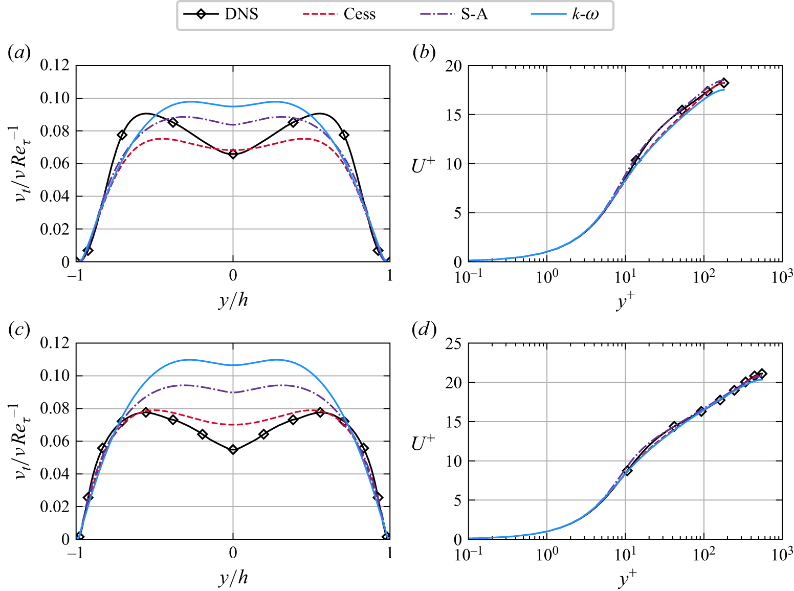
Although the eddy-viscosity enhanced resolvent-based method is widely employed, the approach requires the eddy viscosity and the mean velocity to be known a priori. For turbulent channel flows, the Cess model (Cess Reference Cess1958; Reynolds & Tiederman Reference Reynolds and Tiederman1967) is often used to provide the eddy-viscosity profile, and the mean velocity is further obtained by solving the Reynolds-averaged Navier–Stokes (RANS) equation under the Boussinesq assumption. However, the Cess model is limited to channel and pipe flows, necessitating the commonly used turbulence model, e.g. Spalart–Allmaras model (Spalart & Allmaras Reference Spalart and Allmaras1992) and
 $k$
–
 $\omega$
model (Wilcox Reference Wilcox1998), for general applications including jet and airfoil flows (von Saldern et al. Reference von, Jakob, Schmidt, Jordan and Oberleithner2024). Furthermore, these eddy-viscosity models have intrinsic uncertainties to represent the Reynolds stress in the RANS equation (Duraisamy, Iaccarino & Xiao Reference Duraisamy, Iaccarino and Xiao2019), making it challenging to generalise well across different flow scenarios. Such uncertainties in the RANS-provided eddy viscosity can also significantly affect the predictive accuracy of the eddy-viscosity enhanced resolvent-based method in the velocity spectra. On the other hand, the eddy-viscosity enhanced resolvent-based method still can not fully recover the velocity statistics, particularly in the time correlation (Wu & He Reference Wu and He2023), due to the white-in-time stochastic excitation. Therefore, the nonlinear forcing model is worthy of further development to improve the predictive performance of the resolvent-based method enhanced with the RANS-provided eddy viscosity.
Data-driven approaches have been explored to improve the nonlinear forcing model by optimising either the eddy-viscosity profile or the magnitude of white-noise stochastic forcing based on high-fidelity data. For instance, Pickering et al. (Reference Pickering, Rigas, Schmidt, Sipp and Colonius2021a ) determined the optimal eddy viscosity by aligning the dominant resolvent mode with the spectral proper orthogonal decomposition (SPOD) mode of data from large-eddy simulations. This can achieve the best possible predictions of velocity responses with the eddy-viscosity enhanced resolvent framework. Moreover, the optimised eddy viscosity can improve the transfer function from nonlinear forcings to their linear responses for flow control applications. Alternatively, Holford et al. (Reference Holford, Lee and Hwang2023) optimised the magnitude of directionally dependent white-noise forcing based on the DNS data, thereby improving the prediction of the turbulent Reynolds stresses. These approaches can produce optimal nonlinear forcing fields while tailored to specific flow configurations, limiting their generalisability to other flow conditions and RANS models.
Neural-network-based function approximation has exhibited remarkable potential in developing generalisable turbulence models associated with Reynolds stress (Ling & Templeton Reference Ling and Templeton2015; Zhang et al. Reference Zhang, Xiao, Luo and He2022) and subgrid-scale stress (Zhou et al. Reference Zhou, He, Wang and Jin2019; Park & Choi Reference Park and Choi2021). In particular, neural operators (Kovachki et al. Reference Kovachki, Li, Liu, Azizzadenesheli, Bhattacharya, Stuart and Anandkumar2023) can learn mappings between infinite function spaces from high-fidelity data, enabling generalisation across diverse model inputs. The deep operator network (DeepONet) (Lu et al. Reference Lu, Jin, Pang, Zhang and Karniadakis2021) is one widely used neural operator composed of two subnetworks, where a branch net is used to encode the input function and a trunk net is used to encode the domain location of the output function to be evaluated. This architecture has been successfully applied to various flow applications, such as learning turbulent combustion closure (Taassob et al. Reference Taassob, Kumar, Gitushi, Ranade and Echekki2024), building surrogate models of bubble dynamics (Lin et al. Reference Lin, Maxey, Li and Karniadakis2021), predicting instability waves in high-speed boundary layers (Di Leoni et al. Reference Di, Clark, Lu, Meneveau, Karniadakis and Zaki2023), accelerating data assimilation for transitional flows over a cone (Morra, Meneveau & Zaki Reference Morra, Meneveau and Zaki2024) and modelling multiphysics fields of hypersonic reacting flows (Mao et al. Reference Mao, Lu, Marxen, Zaki and Karniadakis2021; Cai et al. Reference Cai, Wang, Lu, Zaki and Karniadakis2021). Moreover, the DeepONet is flexible to augment the output function domain (Lu et al. Reference Lu, Meng, Cai, Mao, Goswami, Zhang and Karniadakis2022). Given these strengths, the DeepONet-based neural operator is promising to build data-driven nonlinear forcing models that improve the generalisability of resolvent-based methods across different RANS models and flow conditions.
In this work we propose the neural operator-based nonlinear forcing model for predicting the space–time statistics of large-scale structures in turbulent channel flows. The approach integrates the eddy-viscosity enhanced resolvent operator and the neural operator-based stochastic forcing model. Specifically, the DeepONet-based model is built to map the eddy viscosity and mean velocity to the stochastic forcing spectra based on the DNS data. The stochastic forcing is considered direction dependent, non-uniform in the wall-normal direction and correlated in both space and time. Furthermore, the obtained stochastic forcing can yield the space–time velocity statistics via the eddy-viscosity enhanced resolvent operator. In doing so, the proposed model can produce the coloured-in-time stochastic forcing, enabling accurate prediction of space–time statistics of large-scale flow structures. Particularly, the neural operator-enhanced resolvent model allows for predicting velocity spectra based on the RANS-provided mean velocity and eddy viscosity, without requiring available data. As such, the learned model can be applied to similar flow conditions, e.g. with varying Reynolds numbers. Moreover, the DeepONet-based forcing model can be well generalised for different eddy-viscosity profiles and the corresponding mean velocity, providing relatively consistent predictions in velocity statistics.
The rest of the paper is structured as follows. The problem of modelling stochastic forcing for the resolvent-based method is first illustrated in § 2. Afterward, the proposed resolvent neural operator is presented in § 3. The data generation for training the neural operator is described in § 4. Furthermore, the predictive performance of the learned stochastic forcing model in terms of forcing statistics, velocity statistics and model generalisability is evaluated and discussed in § 5. Finally, the paper is concluded in § 6.
2. Problem formulation
2.1. Resolvent operator
The mathematical description of the resolvent-based method is introduced for turbulent channel flows. The linearised Navier–Stokes equations for incompressible turbulent channel flows, with turbulent Reynolds stresses modelled based on eddy viscosity, are given as (Reynolds & Hussain Reference Reynolds and Hussain1972; Cossu, Pujals & Depardon Reference Cossu, Pujals and Depardon2009)
 \begin{align} \boldsymbol{\nabla }\boldsymbol{\cdot }\boldsymbol{u}&=0, \end{align}
 \begin{align} \partial _t\boldsymbol{u}+\boldsymbol{U}\boldsymbol{\cdot }\boldsymbol{\nabla }\boldsymbol{u}+\boldsymbol{u}\boldsymbol{\cdot }\boldsymbol{\nabla }\boldsymbol{U}+\boldsymbol{\nabla }p &=\boldsymbol{\nabla }\boldsymbol{\cdot }\Big [\big (\nu +\nu _t\big )\big (\boldsymbol{\nabla }\boldsymbol{u}+\boldsymbol{\nabla }\boldsymbol{u}^\top \big )\Big ]+\boldsymbol{f} {,} \end{align}
where
 $\boldsymbol{u}= [u(\boldsymbol{x},t),v(\boldsymbol{x},t),w(\boldsymbol{x},t) ]^\top$
denotes the fluctuating velocity field. The domain is represented by Cartesian coordinates
 $\boldsymbol{x}=(x,y,z)^\top$
, corresponding to the streamwise (
 $x$
), wall-normal (
 $y$
) and spanwise (
 $z$
) directions. The mean velocity
 $\boldsymbol{U}= [U(y),0,0 ]^\top$
has only a streamwise component, which varies in the wall-normal direction
 $y\in [-h,h ]$
, with
 $h$
being the channel half-height. The variables
 $p$
,
 $\nu$
and
 $\nu _t$
represent the fluctuating pressure, kinematic viscosity and eddy viscosity, respectively. The stochastic forcing
 $\boldsymbol{f}$
accounts for the deficit between the eddy-viscosity term and the exact nonlinear term (Holford et al. Reference Holford, Lee and Hwang2023), which is defined as
 \begin{equation} \boldsymbol{f}\equiv -\boldsymbol{\nabla }\boldsymbol{\cdot }\left (\boldsymbol{uu}-\langle \boldsymbol{uu}\rangle \right )-\boldsymbol{\nabla }\boldsymbol{\cdot }\Big [\nu _t\big (\boldsymbol{\nabla }\boldsymbol{u}+\boldsymbol{\nabla }\boldsymbol{u}^\top \big )\Big ] {,} \end{equation}
with
 $\langle \boldsymbol{\cdot }\rangle$
denoting an ensemble average.
Owing to the homogeneity of the channel flow in the wall-parallel (
 $x$
–
 $z$
) plane, (2.1) can be Fourier transformed in these directions. Furthermore, the standard pressure elimination procedures (Schmid, Henningson & Jankowski Reference Schmid, Henningson and Jankowski2002) are applied to yield the evolution equation as
 \begin{equation} \frac {\partial }{\partial t}\hat {\boldsymbol{q}}(\boldsymbol{k},y,t)=\boldsymbol{A}_{\nu _t}\hat {\boldsymbol{q}}(\boldsymbol{k},y,t)+\boldsymbol{B} \kern3pt \hat{\boldsymbol{\kern-3pt f}}(\boldsymbol{k},y,t) {,} \end{equation}
where
 $\hat {\boldsymbol{q}}= [\hat {v},\hat {\omega }_y ]$
is the state vector involving the Fourier modes of the wall-normal velocity and wall-normal vorticity. The wavenumber vector is given by
 $\boldsymbol{k}= (k_x, k_z )$
, where
 $k_x$
and
 $k_z$
represent the streamwise and spanwise wavenumbers, respectively. The velocity vector and state vector are related through
 $\hat {\boldsymbol{u}}=\boldsymbol{C}\hat {\boldsymbol{q}}$
and
 $\hat {\boldsymbol{q}}=\boldsymbol{D}\hat {\boldsymbol{u}}$
, where
 $\boldsymbol{C}$
and
 $\boldsymbol{D}$
are transformation matrices. Further considering the statistical stationarity of the flow over time, the dynamic system in (2.3) can be Fourier transformed in time, yielding the velocity response to stochastic forcing as
 \begin{equation} \tilde {\boldsymbol{u}}\left (\boldsymbol{k},\omega ,y\right )=\boldsymbol{R}\kern3pt \tilde{\boldsymbol{\kern-3pt f}}\left (\boldsymbol{k},\omega ,y\right )\!{,} \end{equation}
where
 $\omega$
is the frequency,
 $\tilde {\boldsymbol{u}}$
and
 $\kern3pt \tilde{\boldsymbol{\kern-3pt f}}$
are the Fourier modes of velocity and stochastic forcing vectors, respectively, and
 $\boldsymbol{R}$
is the resolvent operator defined as
 \begin{equation} \boldsymbol{R}=-\boldsymbol{C}\left ({\textrm{i}}\omega \boldsymbol{I}+\boldsymbol{A}_{\nu _t}\right )^{-1}\boldsymbol{B} {.} \end{equation}
Here
 ${\textrm{i}}$
is the imaginary unit and
 $\boldsymbol{I}$
is the identity matrix. For each wavenumber and frequency, (2.4) is discretised in the wall-normal direction, using
 $N_y$
Chebyshev collocation points. The boundary conditions are imposed at both walls as
 $\tilde {v}(\pm h)=\partial _y\tilde {v}(\pm h)=\tilde {\omega }_y (\pm h )=0$
. The vectors
 $\tilde {\boldsymbol{u}}$
and
 $\kern3pt \tilde{\boldsymbol{\kern-3pt f}}$
, each of size
 $3N_y\times 1$
, include the Fourier modes of the velocity and stochastic forcing components, respectively. Detailed formulations of the matrices
 $\boldsymbol{A}_{\nu _t},\boldsymbol{B},\boldsymbol{C}$
and
 $\boldsymbol{D}$
are provided in Appendix A. The resolvent operator
 $\boldsymbol{R}$
incorporates both the eddy-viscosity profile
 $\nu _t(y)$
and the mean flow profile
 $U(y)$
, which are obtained by solving the RANS equations using the eddy-viscosity-based turbulence models (Pope Reference Pope2000). Several turbulence models are available for this purpose in channel flows, including the Cess model (Cess Reference Cess1958; Reynolds & Tiederman Reference Reynolds and Tiederman1967), the Spalart–Allmaras model (Spalart & Allmaras Reference Spalart and Allmaras1992) and the
 $k$
–
 $\omega$
model (Wilcox Reference Wilcox1998, Reference Wilcox2008), as briefly illustrated in Appendix B.
Given the eddy viscosity and mean velocity, the resolvent operator
 $\boldsymbol{R}$
can be obtained based on (2.5). Furthermore, provided a modelled stochastic forcing, the velocity cross-spectra can be derived from (2.4) as
 \begin{equation} \boldsymbol{S}=\boldsymbol{RPR}^{{H}} {,} \end{equation}
where
 $\boldsymbol{S}$
and
 $\boldsymbol{P}$
are the cross-spectra of velocity and stochastic forcing, respectively. They can be formulated as
 \begin{equation} \begin{aligned} \boldsymbol{S}(k_x,k_z,\omega ,y,y')&=\langle {\tilde {\boldsymbol{u}}(k_x,k_z,\omega ,y)\tilde {\boldsymbol{u}}^H(k_x,k_z,\omega ,y')}\rangle ,\\ \boldsymbol{P}(k_x,k_z,\omega ,y,y')&=\langle {\kern3pt \tilde{\boldsymbol{\kern-3pt f}}(k_x,k_z,\omega ,y){\kern3pt \tilde{\boldsymbol{\kern-3pt f}}^H}(k_x,k_z,\omega ,y')}\rangle {,} \end{aligned} \end{equation}
where the superscript
 ${H}$
denotes the conjugate transpose (Hermitian transpose). For notation convenience, the dependency on wavenumbers and frequency is omitted hereafter. The Hermitian matrices
 $\boldsymbol{S}$
and
 $\boldsymbol{P}$
are both block structured matrices as
 \begin{equation} \boldsymbol{S}=\left [ \begin{array}{c|c|c} \langle \tilde {u}\tilde {u}^{{H}}\rangle & \langle \tilde {u}\tilde {v}^{{H}}\rangle & \langle \tilde {u}\tilde {w}^{{H}}\rangle \\[2pt] \hline \\[-9pt] \langle \tilde {v}\tilde {u}^{{H}}\rangle & \langle \tilde {v}\tilde {v}^{{H}}\rangle & \langle \tilde {v}\tilde {w}^{{H}}\rangle \\[2pt] \hline \\[-9pt] \langle \tilde {w}\tilde {u}^{{H}}\rangle & \langle \tilde {w}\tilde {v}^{{H}}\rangle & \langle \tilde {w}\tilde {w}^{{H}}\rangle \\ \end{array}\right ],\quad \boldsymbol{P}=\left [ \begin{array}{c|c|c} \langle \tilde {f}_x\tilde {f}_x^{{H}}\rangle & \langle \tilde {f}_x\tilde {f}_y^{{H}}\rangle & \langle \tilde {f}_x\tilde {f}_z^{{H}}\rangle \\[2pt] \hline \\[-9pt] \langle \tilde {f}_y\tilde {f}_x^{{H}}\rangle & \langle \tilde {f}_y\tilde {f}_y^{{H}}\rangle & \langle \tilde {f}_y\tilde {f}_z^{{H}}\rangle \\[2pt] \hline \\[-9pt] \langle \tilde {f}_z\tilde {f}_x^{{H}}\rangle & \langle \tilde {f}_z\tilde {f}_y^{{H}}\rangle & \langle \tilde {f}_z\tilde {f}_z^{{H}}\rangle \end{array} \right ]. \end{equation}
The block matrices
 $\boldsymbol{S}$
and
 $\boldsymbol{P}$
consists of
 $3\times 3$
submatrices
 $S_{ij}=\langle \tilde {u}_i\tilde {u}_j^{{H}}\rangle$
and
 $P_{ij}=\langle \tilde {f}_i\tilde {f}_j^{{H}}\rangle$
for
 $i,j=1,2,3$
, each of size
 $N_y\times N_y$
. Within each submatrix, the diagonal elements represent the one-point correlation of the corresponding vector components, while the off-diagonal elements describe the wall-normal correlations. Conclusively, the cross-spectra
 $\boldsymbol{S}$
of velocity can be obtained from the forcing spectra
 $\boldsymbol{P}$
via the resolvent operator.
2.2. Prescribing stochastic forcing spectra
In order to model the stochastic forcing, it is vital to prescribe the statistical structure of the forcing. The stochastic forcing
 $\boldsymbol{f}$
in (2.2) is known to be coloured-in-time, scale-dependent, spatially correlated in the wall-normal direction, cross-correlated among its components and non-uniform in intensity across the channel height (Holford et al. Reference Holford, Lee and Hwang2023). The stochastic forcing in this work is assumed as spatially decorrelated with an absence of cross-component correlation, following previous studies (Morra et al. Reference Morra, Semeraro, Henningson and Cossu2019, Reference Morra, Nogueira, Cavalieri and Henningson2021; Gupta et al. Reference Gupta, Madhusudanan, Wan, Illingworth and Juniper2021; Holford et al. Reference Holford, Lee and Hwang2023, Reference Holford, Lee and Hwang2024). In doing so, the forcing spectra
 $\boldsymbol{P}$
to be modelled is simplified from a full
 $3N_y\times 3N_y$
matrix to its diagonal elements of a size
 $3N_y$
.
In this work we prescribe the stochastic forcing to be coloured-in-time and scale-dependent with varying intensity across wall-normal locations while conserving kinetic energy. Specifically, the target stochastic forcing spectra is formulated as
 \begin{equation} \boldsymbol{P}(\boldsymbol{k},\omega ,y,y')=\gamma (\boldsymbol{k},\omega )\boldsymbol{W}(\boldsymbol{k},\omega ,y)\delta \left (y-y'\right ) {,} \end{equation}
where
 $\boldsymbol{P}$
is a diagonal matrix that excludes both the wall-normal correlation and the cross-component correlation, retaining only the one-point autocorrelation at specified wavenumbers and frequencies. The matrix
 $\boldsymbol{W}$
represents the relative intensity distribution in the wall-normal direction, which can be obtained from the one-point autocorrelations of the solenoidal part of the stochastic forcing. The coefficient
 $\gamma$
is used to scale the forcing intensity to match the DNS-predicted kinetic energy. The coefficient
 $\gamma$
and matrix
 $\boldsymbol{W}$
are determined as
 \begin{equation} \gamma \left (\boldsymbol{k},\omega \right )=\frac {\| \boldsymbol{S}^{\textit{(DNS)}}\|_*}{\| \boldsymbol{R}\boldsymbol{W}\boldsymbol{R}^{{H}} \|_*},\quad \boldsymbol{W}=\big (\boldsymbol{L}\boldsymbol{S}^{\textit{(DNS)}}\boldsymbol{L}^{{H}}\big )\circ \boldsymbol{I} {.} \end{equation}
Here
 $\circ$
denotes the element-wise matrix product (Hadamard product) and
 $\|\boldsymbol{\cdot }\|_*$
is the nuclear norm (Bhatia Reference Bhatia1997) defined as
 \begin{equation} \|\boldsymbol{S}\|_*:= \sum _{i=1}^{3N_y}\sigma _i(\boldsymbol{S}), \end{equation}
which is given by the summation of all singular values
 $\sigma _i(\boldsymbol{S})$
. Owing to the orthogonality of the singular vectors, the nuclear norm
 $\|\boldsymbol{S}\|_*$
of the velocity cross-spectra matrix
 $\boldsymbol{S}$
represents twice the turbulent kinetic energy integrated over the wall-normal direction at a given wavenumber and frequency (Jovanović & Bamieh Reference Jovanović and Bamieh2005), i.e.
 \begin{equation} \|\boldsymbol{S}\|_*=\iint _{-h}^{h}\sum _{i=1}^{3}\langle \tilde {u}_i(y)\tilde {u}_i^{{H}}(y')\rangle \delta (y-y'){\textrm{d}}{y}{\textrm{d}}{y'}. \end{equation}
This formula is used to compute the nuclear norm in practice. The operator
 $\boldsymbol{L}$
in (2.10) is defined as (Morra et al. Reference Morra, Semeraro, Henningson and Cossu2019)
 \begin{equation} \boldsymbol{L}=-\boldsymbol{C}\left ({\textrm{i}}\omega \boldsymbol{I}+\boldsymbol{A}_{\nu _t}\right )\boldsymbol{D}, \end{equation}
which is used to recover the solenoidal part of the stochastic forcing, i.e.
 \begin{equation} \boldsymbol{L}\tilde {\boldsymbol{u}}={\kern3pt \tilde{\boldsymbol{\kern-3pt f}}^{s}}. \end{equation}
Note that the stochastic forcing can be decomposed into a solenoidal part and an irrotational part, i.e.
 \begin{equation} \kern3pt \tilde{\boldsymbol{\kern-3pt f}}={\kern3pt \tilde{\boldsymbol{\kern-3pt f}}^{s}}+{\kern3pt \tilde{\boldsymbol{\kern-3pt f}}^{r}}, \end{equation}
where the solenoidal part is divergence free (i.e.
 $\boldsymbol{\nabla }\boldsymbol{\cdot }{\kern3pt \tilde{\boldsymbol{\kern-3pt f}}^{s}}=0$
) and the irrotational part is curl free (i.e.
 $\boldsymbol{\nabla }\times {\kern3pt \tilde{\boldsymbol{\kern-3pt f}}^{r}}=0$
). Since the irrotational forcing
 $\boldsymbol{f}^{{r}}$
resides in the null space of operator
 $\boldsymbol{B}$
(Rosenberg & McKeon Reference Rosenberg and McKeon2019), only the solenoidal components of stochastic forcing can be recovered from velocity. Conclusively, in this work we aim to model the one-point autocorrelation
 $\boldsymbol{P}$
of the stochastic forcing defined in (2.9).
3. Methodology
3.1. Neural operator for modelling stochastic forcing
The neural operator is introduced to model the frequency spectra of stochastic forcing components. Based on (2.14), the stochastic forcing is related to the mean velocity and eddy viscosity given the accurate fluctuating velocity response
 $\tilde {\boldsymbol{u}}$
from the DNS. In view of this, we assume that the stochastic forcing is a function of the mean velocity and the eddy viscosity, which can be approximated using the neural operator method.
The DeepONet-based neural operator is employed to represent the stochastic forcing spectra. The neural operator has an appealing property that its input and output functions need not share the same domain, enabling mappings between arbitrary function spaces (Lu et al. Reference Lu, Meng, Cai, Mao, Goswami, Zhang and Karniadakis2022). By leveraging this flexibility, we construct a neural operator where the input functions are defined over the non-dimensional wall distance
 $1-| y|/h$
, while the output functions are extended to the wavenumber–frequency–distance domain
 $(k_xh,k_zh,\omega h/U_{{m}},1-| y|/h)$
. Specifically, the inputs consist of two profiles, i.e. mean velocity and eddy viscosity along the wall-normal direction, and the outputs consist of three frequency spectra corresponding to the components of the stochastic forcing. Following the work of Lu et al. (Reference Lu, Meng, Cai, Mao, Goswami, Zhang and Karniadakis2022), we employ an extended version of DeepONet capable of handling multiple input and output functions. As shown in figure 1, the neural network is composed of a branch network and a trunk network. The input layer of the branch network is split into two groups, separately encoding the mean velocity profile and the eddy-viscosity profile. The trunk network takes inputs as a set of location points to evaluate the output function of forcing spectra, including streamwise and spanwise wavenumbers
 $(k_x, k_z)$
, temporal frequency
 $\omega$
and the wall-normal distance
 $1-|y|/h$
. The output layer of the branch network is divided into three groups
 $\boldsymbol{b}_i= [{b}_{i1},{b}_{i2},\boldsymbol{\cdots} ,{b}_{in} ]^\top$
with
 $i=1,2,3$
, each corresponding to one component of the stochastic forcing and having the same dimension as the output of the trunk network
 $\boldsymbol{a} = [{a}_1,{a}_2,\boldsymbol{\cdots} ,{a}_n ]^\top$
, where
 $n$
is the dimension of the trunk net output. The outputs of the branch network are combined with the trunk network output via inner products to yield the frequency spectra of the three stochastic forcing components, i.e.
 $P_{ii}=\sum _{j=1}^{n}{a}_{j}{b}_{ij}$
. The input mean velocity profile and query points are non-dimensionalised using the outer characteristic velocity scale of the mean bulk velocity
 $U_{{m}}$
and length scale of the channel half-height
 $h$
, respectively. This dimensionless method is chosen because large-scale motions at different Reynolds numbers have similar characteristic scales when measured in outer units (Cossu & Hwang Reference Cossu and Hwang2017). The input eddy viscosity is non-dimensionalised as
 $\nu _t/\nu Re_\tau ^{-1}$
, since this scaling allows the eddy-viscosity profiles to align closely across different Reynolds numbers (Symon et al. Reference Symon, Madhusudanan, Illingworth and Marusic2023).
The architecture of the DeepONet-based neural operator for modelling the stochastic forcing spectra. The DeepONet consists of a branch network and a trunk network. The branch network takes the input profiles
 $U(y)$
and
 $\nu _t(y)$
, while the trunk network processes the wavenumber–frequency–position tuple
 $(k_x h,k_z h,\omega h/U_{{m}},1-| y|/h)$
. The branch output is split into three groups, each combined with the trunk output via inner products to produce three components of the output functions
 $P_{ii},i=1,2,3$
.

3.2. Neural operator-enhanced resolvent prediction
We propose the neural operator-enhanced resolvent model to predict the velocity spectra in turbulent channel flows. It is achieved by integrating the linear resolvent operator with a neural operator-based stochastic forcing. Specifically, the DeepONet-based neural operator takes the mean velocity and eddy viscosity as the model input and yields the frequency spectra of the coloured-in-time stochastic forcing at different wavenumbers and wall-normal positions. Furthermore, the obtained forcing spectra can be propagated to the velocity responses via the resolvent operator. As such, the learned neural operator combined with the resolvent operator can map the RANS-provided eddy viscosity and mean velocity to the velocity spectra at characteristic scales of large-scale flow structures.
A schematic is plotted in figure 2 to illustrate the proposed neural operator-enhanced resolvent model. Specifically, the RANS method coupled with turbulence models is first used to provide the eddy viscosity
 $\nu _t$
and the corresponding mean velocity
 $U$
. On the one hand, the obtained mean velocity and eddy viscosity are used to determine the eddy-viscosity enhanced resolvent operator
 $\boldsymbol{R}$
based on (2.5). On the other hand, they are used as the inputs of the DeepONet-based forcing model, which produces the forcing spectra
 $\boldsymbol{P}$
at the location points to be evaluated. Finally, the velocity spectra can be obtained via the inner products of the resolvent operator
 $\boldsymbol{R}$
and the forcing spectra
 $\boldsymbol{P}$
predicted by the neural operator. The proposed forcing model is capable of accurately predicting fluctuating velocity spectra independent of the RANS model. Moreover, such an approach circumvents the need for available velocity data, such as sweeping velocities or eddy-damping length scales required in the sweep-enhanced forcing model (Wu & He Reference Wu and He2023).
Schematic plot of the velocity spectra predicted with the neural operator-based coloured-in-time forcing. The RANS module provides the eddy viscosity
 $\nu _t$
and mean velocity
 $U$
to construct both the resolvent operator
 $\boldsymbol{R}$
and the neural operator-based forcing. The learned neural operator predicts the stochastic forcing spectra
 $\boldsymbol{P}$
, which is combined with the resolvent operator
 $\boldsymbol{R}$
to generate the velocity spectra
 $\boldsymbol{S}$
.

The neural-network architecture of the DeepONet-based forcing model is described as follows. The trunk net takes a 4-dimensional input, processes it through 12 hidden layers with 192 neurons each (using ReLU activation) and produces a 64-dimensional output. The branch net has a 130-dimensional input, passes it through an identical hidden structure (12 layers
 $\times$
192 neurons, ReLU-activated) and produces a 192-dimensional output. The code used for this work and the learned stochastic forcing model are publicly accessible (Wu et al. Reference Wu, Zhang and He2025a
). Note that the predictive reliability of neural networks can be limited by their black-box nature. In spite of this, the neural network is of great interest to extract underlying functional mapping from high-fidelity data, given its nonlinear expressive power and high training efficiency. The interpretability can be further obtained with explainability techniques, such as the feature importance analysis and the symbolic learning method. For instance, one can quantify the contribution of each input feature to the learned functional mapping based on the Shapley additive explanations (Lundberg & Lee Reference Lundberg and Lee2017; Wu et al. Reference Wu, Wang, Zhang and He2023), highlighting the most influential features. Alternatively, the black-box functional mapping can be transformed into interpretable white-box models using symbolic regression (Wu et al. Reference Wu, Zhang, Xu and He2025b
).
In this work we aim to improve the modelling of the stochastic forcing instead of the eddy viscosity. Improving eddy viscosity can also enhance the resolvent-based prediction from two aspects. On the one hand, the eddy viscosity is related to the mean velocity via the RANS equations. Improving the RANS-based eddy viscosity can provide an accurate mean velocity in the linear operator. On the other hand, the eddy viscosity is used to model partially the nonlinear forcing and enhance the resolvent-based linear operator. One can optimise the eddy viscosity to have the best alignment between the leading resolvent mode and the SPOD mode of high-fidelity data (Pickering et al. Reference Pickering, Rigas, Schmidt, Sipp and Colonius2021a ). However, with the optimal eddy viscosity, the velocity response can still exhibit large discrepancies, particularly in the spectral domain. This is because the provided eddy viscosity is not a function of wavenumber or frequency, which contradicts the fact that the mapping from velocity to nonlinear terms is inherently scale by scale (Ying et al. Reference Ying, Chen, Li and Fu2024). Also, the eddy-viscosity enhanced linear model yields velocity spectra with an infinite frequency bandwidth with white-noise forcing, resulting in vanishing Taylor time microscales. Furthermore, it has been noted by Russo & Luchini (Reference Russo and Luchini2016) that no eddy-viscosity model can reproduce accurately the velocity response to a volume force. For these reasons, this work mainly focuses on the modelling of stochastic forcing, instead of eddy viscosity. The model errors from the nonlinear forcing and mean velocity are compensated in the stochastic forcing in the present work. In doing so, the coloured-in-time nonlinear forcing can be fully recovered to provide accurate velocity spectra. In addition, the neural operator is introduced to build the functional mapping from different RANS inputs to the corresponding stochastic forcing. As such, the nonlinear forcing can be relatively independent of the RANS model inputs through accounting for the uncertainty in the RANS-provided eddy viscosity.
4. Data generation
4.1. Direct numerical simulation
To train the neural operator model, we perform DNS to provide the training data for the stochastic forcing spectra. The computational domain extends over
 $L_x, 2h, L_z$
in the streamwise, wall-normal and spanwise directions, respectively. Periodic boundary conditions are imposed in the wall-parallel directions and the no-slip no-penetration boundary conditions are applied at both the upper and bottom walls. The temporal discretisation is employed by a third-order, multi-step, stiffly stable method (Karniadakis, Israeli & Orszag Reference Karniadakis, Israeli and Orszag1991). The nonlinear convective terms are approximated using an explicit third-order Adams–Bashforth scheme (Willoughby Reference Willoughby1973), and the viscous terms are approximated using an implicit third-order Adams-Moulton scheme (Willoughby Reference Willoughby1973). For spatial discretisation, flow variables are discretised via the Fourier series in the streamwise and spanwise directions and the Chebyshev polynomials in the wall-normal direction. To mitigate the aliasing error in the nonlinear terms, the
 $3/2$
rule (Orszag Reference Orszag1971b
) is applied. The simulation is carried out with
 $N_x\times N_y\times N_z$
mesh points. A two-dimensional decomposition parallel strategy (Lee, Malaya & Moser Reference Lee, Malaya and Moser2013) is employed to partition the three-dimensional domain along two axes with the message passing interface (MPI). To compute the nonlinear terms with a dealiased fast Fourier transform and inverse fast Fourier transform (FFT/IFFT) on the
 $x$
–
 $z$
planes, data are transposed between processes for both the forward and inverse transforms to align with the FFT dimension. Simulations are conducted on
 $128$
MPI processes for
 $Re_\tau =180$
and
 $384$
processes for
 $Re_\tau =550$
. The compute server used is equipped with six AMD EPYC 7662 CPUs (64 cores/CPU,
 ${2.0}\,\textrm {GHz}$
base clock, hyper-threading disabled), providing 384 processes.
In this work the DNS data from two channel flow cases are used, corresponding to friction Reynolds numbers of
 $Re_\tau =180$
and
 $Re_\tau =550$
. Here,
 $Re_\tau =u_\tau h/\nu$
is defined based on the friction velocity
 $u_\tau$
and the channel half-height
 $h$
. The flow data of
 $Re_\tau =180$
is used to train the neural operator model and the data of
 $Re_\tau =550$
is used to test the generalisability of the learned model. The details of the case set-up are illustrated in table 1. The comparison of mean velocity and Reynolds normal stresses between the present DNS and the reference data (Lee & Moser Reference Lee and Moser2015) is presented in figure 3. The mean velocity and Reynolds stresses are plotted in viscous units, which exhibit good agreement with the results of Lee & Moser (Reference Lee and Moser2015). The temporal Fourier transform is computed using a windowed FFT, with details provided in Appendix C. The DNS solver and the data processing have been validated in previous studies (Wu & He Reference Wu and He2020, Reference Wu and He2021, Reference Wu and He2023).
Case set-up of the DNS for generating high-fidelity data. The case of
 $Re_\tau =180$
is used for training the neural operator model, while the case of
 $Re_\tau =550$
is for the generalisability test. Here
 $L_x$
and
 $L_z$
represent the computational domain sizes in streamwise and spanwise directions, respectively;
 $\Delta _x^+$
and
 $\Delta _z^+$
are the corresponding grid spacings in the wall-parallel direction;
 $\Delta y_w^+$
and
 $\Delta y_c^+$
are the wall-normal grid spacing at the wall and channel centre;
 $\Delta t$
denotes the time step. The scale with notation
 $^+$
is measured in wall units.

Comparison of the present DNS results (solid lines) with reference data (marker symbols) from Lee & Moser (Reference Lee and Moser2015) at
 $Re_\tau =180$
(grey) and
 $550$
(black). (a) Mean velocities
 $U^+$
; (b) Reynolds normal stresses:
 $\langle uu\rangle ^+$
,
 $\langle vv\rangle ^+$
and
 $\langle ww\rangle ^+$
.

4.2. Characteristic scales in channel flows
Turbulent flows exhibit pronounced scale separation (Smits, McKeon & Marusic Reference Smits, McKeon and Marusic2011), which poses a significant challenge for modelling all flow scales. Coherent structures at characteristic scales have been recognised as essential to the self-sustaining process (Cossu & Hwang Reference Cossu and Hwang2017). Therefore, in this work we aim to predict velocity spectra at the characteristic scales associated with self-sustaining energy-containing motions using the proposed neural operator model.
Various flow structures at characteristic scales have been identified to reveal the self-similar nature of large-scale motions (Hwang & Cossu Reference Hwang and Cossu2010c ; Hwang Reference Hwang2015; Cossu & Hwang Reference Cossu and Hwang2017). For instance, the long streaky structures and the short and tall vortical structures (often referred to as hairpin vortex packets) have been identified as two dynamically interconnected energy-containing motions. These motions consistently co-occur, suggesting they are dynamically interconnected elements of a single attached eddy. The long streaks primarily carry streamwise turbulent kinetic energy and exhibit self-similar scaling, with their size and geometry approximated by
 \begin{equation} y\simeq 0.1\lambda _z,\quad \lambda _x\simeq 10\lambda _z {,} \end{equation}
where
 $\lambda _x=2\pi /k_x$
and
 $\lambda _z=2\pi /k_z$
denote the streamwise and spanwise wavelengths, respectively. The short and tall vortex packets contribute to turbulent kinetic energy across each velocity component, which can be characterised by
 \begin{equation} y\simeq 0.5\sim 0.7\lambda _z,\quad \lambda _x\simeq 2\sim 3 \lambda _z {.} \end{equation}
The spanwise length scale
 $\lambda _z \simeq 1.5h$
corresponds to the peak location of the spanwise premultiplied spectrum for streamwise velocity
 $k_z\langle \hat {u}\hat {u}^{{H}}\rangle$
in an overdamped LES where small-scale structures are quenched (Hwang & Cossu Reference Hwang and Cossu2010c
). The long streaks and the vortex packets at this spanwise scale are referred to as the very-large-scale motions (VLSMs) and the large-scale motions (LSMs) (Hwang & Cossu Reference Hwang and Cossu2010c
; Hwang Reference Hwang2015), respectively, exhibiting the following scales
 \begin{align} y&\simeq 0.15h,\qquad \quad\!\!\!\! \lambda _z\simeq 1.5h,\quad \lambda _x\simeq 15h \quad {(\text{VLSMs})}, \end{align}
 \begin{align} y&\simeq 0.75\sim 1h,\quad\!\!\! \lambda _z\simeq 1.5h,\quad \lambda _x\simeq 3\sim 4 h \quad {(\text{LSMs})}. \end{align}
The characteristic scales of the coherent structures investigated in this work are illustrated in figure 4. The spanwise scale
 $\lambda _z\simeq 1.5h$
corresponds to a spanwise wavenumber of approximately
 $k_zh\simeq 4.2$
. Here, we focus on the spanwise wavenumbers of approximately
 $k_zh\simeq 4\sim 6$
as indicated by the shaded region in figure 4, which is determined by the discrete wavenumbers in the DNS that most closely match the similar scales in (4.3). The short and tall vortex packets align with
 $\lambda _x/\lambda _z=2,2.5,3$
, and the long streaky structures follow
 $\lambda _x/\lambda _z=10$
. These characteristic scales are marked with circles in figure 4. For training data, we select the following scales at
 $Re_\tau =180$
:
 $\boldsymbol{k}h=(0.5,5)$
for the long streaks and
 $\boldsymbol{k}h=(1.5,4.5),(2,6),(2.25,4.5),(2.5,5),(2.75,5.5),(3,6)$
for the short and tall vortex packets, which are marked as red circles in figure 4(a). The marked scales with blue circles at
 $Re_\tau =180$
and
 $550$
are used for generalisation tests of the learned model.
Characteristic scales of the long streaks and the short and tall vortex packets in turbulent channel flows at (a)
 $Re_\tau =180$
and (b)
 $Re_\tau =550$
. Solid lines show aspect ratios
 $\lambda _x/\lambda _z=2,2.5,3,10$
and the grey mesh indicates wavenumber resolution. Circles denote the characteristic scales, where the short and tall vortex packets correspond to
 $\lambda _x/\lambda _z=2,2.5,3$
and long streaky structures correspond to
 $\lambda _x/\lambda _z=10$
. The grey shaded zone indicates the range of spanwise wavenumber investigated in this work. The red circles represent the scales for model training and the blue circles indicate the scales for generalisation tests.

4.3. Training data for neural operator-based forcing model
Here, we outline the procedure for collecting training data to build the neural operator-based forcing model. Each data point is structured as a triplet, i.e.
 \begin{equation} \Bigg [ \underbrace {\frac {U(y)}{U_{{m}}},\frac {1}{Re_\tau }\frac {\nu _t(y)}{\nu },}_{\text{branch net input}}\quad \underbrace {k_xh,k_zh,\frac {\omega h}{U_{{m}}},1-\frac {| y|}{h},}_{\text{trunk net input}}\quad \underbrace {P_{11},P_{22},P_{33}}_{\text{output}}\, \Bigg ]. \end{equation}
The input functions
 $U(y)$
and
 $\nu _t(y)$
are counterparts. In order to construct the mapping between infinite function spaces, arbitrary eddy-viscosity profiles should be sampled to represent the function space. We employ the orthogonal polynomials to achieve this goal by following the work of Lu et al. (Reference Lu, Jin, Pang, Zhang and Karniadakis2021). Specifically, a perturbation
 $\delta (y)$
is added to the Cess eddy-viscosity profiles (described in Appendix B) as
 \begin{equation} \nu _t(y)=\nu _t^{\textit{Cess}}+\delta (y), \end{equation}
with
 $\delta (y)$
generated using modified orthogonal Chebyshev polynomials as (Lu et al. Reference Lu, Jin, Pang, Zhang and Karniadakis2021)
 \begin{equation} \frac {1}{Re_\tau }\frac {\delta (y)}{\nu }=\sum _{n=0}^N a_n \cos \left (\frac {\pi }{2}\frac {y}{h}\right ) \cos \left (n\arccos \frac {y}{h}\right ) {.} \end{equation}
The modulating function
 $\cos (({\pi }/{2})( {y}/{h}) )$
serves to diminish the perturbation magnitude near the walls, avoiding unphysical values, e.g. negative eddy viscosity, and enabling the perturbation vanishing at boundaries so that
 $\nu _t(\pm h)=0$
. Symmetry constraints are satisfied by setting coefficients
 $a_n=0$
for the odd
 $n$
, and the highest polynomial degree is
 $N=16$
. In this work the coefficients are randomly sampled from a uniform distribution (Yin et al. Reference Yin, Zhang, Yu and Karniadakis2022) over the interval
 $ [-\bar {a},\bar {a} ]$
, where
 $\bar {a}=0.012$
is chosen such that the eddy viscosity of both DNS and RANS models are within the coverage of the sampled eddy viscosities.
In this work the neural network is trained on a dataset of 64 sampled eddy-viscosity profiles for
 $Re_\tau =180$
. Figure 5 compares the sampled eddy-viscosity profiles for model training with the eddy-viscosity profiles of the Cess model and the DNS, along with their corresponding mean velocities obtained by solving the RANS momentum equation. The DNS-derived eddy viscosity is determined by projecting the Reynolds shear stress
 $\langle uv\rangle ^{\textit{(DNS)}}$
onto the wall-normal gradient
 $\partial _y U^{\textit{(DNS)}}$
of the mean streamwise velocity, i.e.
 $\langle uv\rangle ^{\textit{(DNS)}}=-\nu _t^{\textit{(DNS)}} \partial _y U^{\textit{(DNS)}}$
. It can be seen that the generated sampled eddy-viscosity profiles and the mean velocity span a range that encompasses the results from both the DNS and the Cess model.
(a) The sampled eddy-viscosity profiles (grey lines) generated by orthogonal polynomials and (b) the corresponding mean velocity profiles. The eddy viscosity and velocity profiles from the DNS (black solid line for
 $Re_{\tau }=180$
and black dashed line for
 $Re_{\tau }=550$
) and Cess model (red dashed line) are also presented for comparison.

With the sampled eddy-viscosity profiles, the target stochastic forcing spectra are obtained using the velocity cross-spectra of the DNS as described in § 2.2. The target stochastic forcing spectra are obtained at different scales for each discrete frequency within the range
 $\omega h/U_{{m}}\in [-20\pi , 20\pi ]$
. We employ a frequency resolution of
 $\Delta \omega h/U_{{m}}=\pi /51.2$
, which yields 2048 discrete frequencies. To have a tractable training dataset size while ensuring adequate sampling, we employ the Ramer–Douglas–Peucker algorithm (Douglas & Peucker Reference Douglas and Peucker2011) for dynamic frequency sampling. This approach provides fine sampling near spectral peaks (where energy is concentrated) and coarser sampling at high frequencies (where energy diminishes). The wall-normal locations are sampled to have the same resolution as the DNS grid points. Due to symmetry considerations, only half of the channel height, i.e. from the wall to the channel centre, is assumed.
Based on the generated data, the DeepONet-based model described in § 3 is trained by minimising the mean squared error of the forcing prediction. The Adam optimiser is used with an initial learning rate of
 $1\times 10^{-3}$
. The learning rate is dynamically adjusted to improve the training convergence by halving it if the validation loss stagnates for 3 consecutive epochs. The training process involves 2000 epochs with a batch size of 2048, and all weights are initialised via Xavier initialisation to achieve faster training convergence (Glorot & Bengio Reference Glorot and Bengio2010).
5. Results
In this section we present the predictive capability of the neural operator in the stochastic forcing and velocity at the characteristic scales of coherent structures in channel flows. We first demonstrate the training performance of the neural operator in the stochastic forcing by comparing it with the target data from DNS. Furthermore, we present the velocity spectra prediction using the learned neural operator and the white-noise stochastic forcing. Subsequently, the predictive performance of the learned model is shown at different wavenumbers with various eddy-viscosity models, including the Cess model, the Spalart–Allmaras model and the
 $k$
–
 $\omega$
model. The details of these RANS models in a turbulent channel flow are presented in Appendix B. Finally, the generalisation test of the learned model is conducted in the turbulent channel flows at the friction Reynolds number
 $Re_\tau =550$
.
5.1. Prediction of stochastic forcing
Figure 6 shows the spectral peak values,
 $\max (\boldsymbol{P})$
, of the stochastic forcing spectra over frequency and wall-normal position for the target and the neural operator-based predictions at
 $Re_\tau =180$
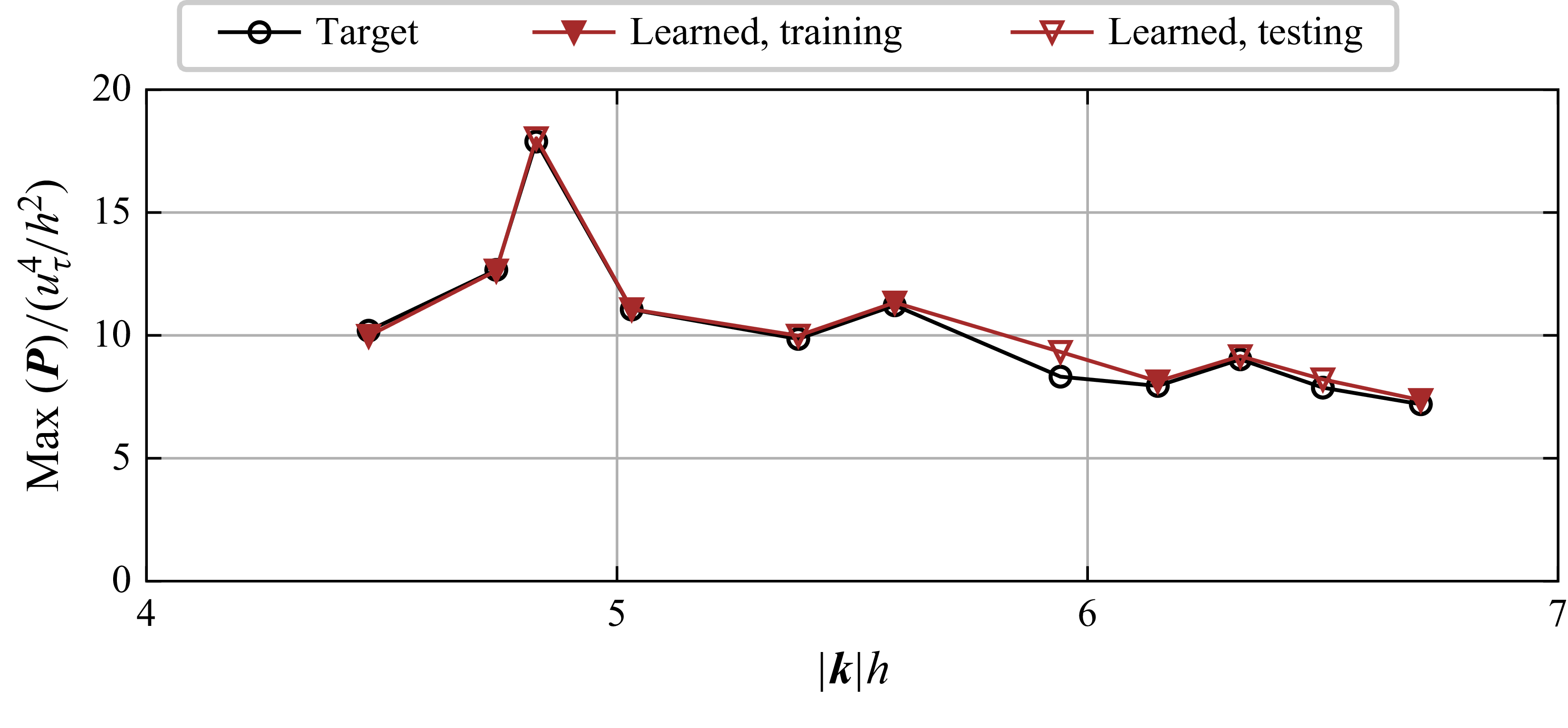
. The results at both training and testing wavenumbers are presented. The learned predictions are obtained by using the eddy viscosity and mean velocity profiles from the Cess model. The learned model accurately captures the spectral peaks across all characteristic scales. A small discrepancy remains only at the testing scale
 $\boldsymbol{k}h=(2.25,5.5)$
, corresponding to
 $| \boldsymbol{k}|h\approx 5.9$
.
The maximum values of the stochastic forcing spectra from the target and the learned predictions at
 $Re_\tau =180$
. Filled and hollow markers denote training and testing wavenumbers, respectively.

Comparison of the frequency spectra
 $P_{ii},(i=1,2,3)$
of stochastic forcing at the wavenumber
 $\boldsymbol{k}h=(2,4)$
for
 $Re_\tau =180$
between (a–c) the target and (d–f) the neural operator predictions using the Cess model. The first (a,d), second (b,e) and third (c,f) columns correspond to the streamwise, wall-normal and spanwise components, respectively. Solid isolines denote the target spectra and dashed isolines denote the predictions of the learned model.

Figure 7 shows the frequency spectra of the stochastic forcing from the target and the learned prediction at the wavenumber
 $\boldsymbol{k}h=(2,4)$
for
 $Re_\tau =180$
. This spanwise wavenumber approximately corresponds to the large-scale structure motions. The forcing spectra
 $P_{ii}$
are normalised by the spectral peak such that the most energetic forcing component has the peak value of 1, presenting the relative distribution of the forcing spectra. Note that the spectra of the white-noise stochastic forcing are constant across all frequencies and wall-normal positions, which hence are not presented for conciseness. It can be seen that the streamwise forcing component dominates in intensity over the wall-normal and spanwise components. The spectra of stochastic forcing reach peaks at wall-normal positions around
 $y^+\simeq 40$
,
 $y^+\simeq 80$
and
 $y^+\simeq 50$
for the streamwise, wall-normal and spanwise components, respectively. The forcing spectral density monotonically decays away from the peak frequency and the peak wall-normal position. The neural operator-based model accurately predicts the peak location in both the frequency and the wall-normal positions. Moreover, the isolines in figure 7 represent different levels evenly spaced on a logarithmic scale between
 $1\times 10^{-3}$
and
 $1$
, which shows that the learned model can accurately capture the decay behaviour in frequency and wall-normal location.
Frequency spectra of the stochastic forcing for
 $Re_\tau =180$
, comparing the forcing spectra
 $P_{ii}$
of the target data and the learned model prediction using the Cess model. The spectra are normalised by their maximum values
 $\max {(\boldsymbol{P})}$
. All plots are at the same spanwise wavenumber
 $k_zh=4.5$
, with streamwise wavenumbers corresponding to scale ratios of (a)
 $\lambda _x/\lambda _z=9$
, (b)
 $3$
, (c)
 $2.5$
and (d)
 $2$
. Each column presents streamwise, wall-normal and spanwise forcing components, respectively. The frequency spectra are evaluated at both the peak wall-normal location and the channel centre. The black dashed line indicates the frequency
 $k_xU_{{m}}$
.

The predictive ability of the neural operator is also examined in terms of the stochastic forcing spectra across different wavenumbers. Figure 8 presents the forcing spectra at a spanwise wavenumber of
 $k_zh=4.5$
and scale ratios
 $\lambda _x/\lambda _z = 9,3,2.5,2$
for flows of the Reynolds number
 $Re_\tau =180$
, compared with the target spectra from the DNS based on (2.9). The comparison is performed at two wall-normal positions, corresponding to the location with maximum spectral intensity and the channel centre, respectively. Notably, the peak frequency of each forcing component is close to
 $k_x U_{{m}}$
across different wavenumbers, which indicates the convection velocity, i.e. the ratio of the peak frequency to the corresponding streamwise wavenumber (del Álamo & Jiménez Reference Hwang and Cossu2009), which aligns with
 $U_{{m}}$
in this case. The streamwise stochastic forcing components dominate over other components by orders of magnitude. The wall-parallel forcing components exhibit significantly lower spectral intensities in the channel centre compared with their peak, and the wall-normal spectra intensities in the channel centre remain close to their peak intensities. At both wall-normal locations, the learned neural operator model can predict the forcing spectra in remarkable agreement with the target data across different wavenumbers.
To quantify the predictive accuracy of the learned neural operator model, we compute the relative error between the target and predicted stochastic forcing spectra as
 \begin{equation} \mathcal{E}_{P_{ii}}= \int _{-\infty }^{\infty }\iint _{-h}^{h} \left | \frac {P_{ii}}{\left [\boldsymbol{P}\right ]}- \frac {P_{ii}^{\textit{(TGT)}}}{\big [\boldsymbol{P}^{\textit{(TGT)}}\big ]} \right |\delta (y-y') {\textrm{d}}{y}{\textrm{d}}{y'}{\textrm{d}}{\omega } {,} \end{equation}
where
 $P_{ii}^{\textit{(TGT)}}$
denotes the target spectra computed based on (2.9),
 $P_{ii}$
represents the neural operator predictions and
 \begin{equation} \left [\boldsymbol{P}\right ] := \int _{-\infty }^{\infty } \|\boldsymbol{P} \|_*{\textrm{d}}{\omega } \end{equation}
is an energy norm (Jovanović & Bamieh Reference Jovanović and Bamieh2005) defined as the integral spectral energy over frequency and wall-normal location at the specified wavenumber. Due to the input–output relationship in (2.6), the velocity responds linearly to the stochastic forcing intensity. Therefore, the error metric defined in (5.1) is used to quantify the relative errors of each forcing component, which is also employed by Holford et al. (Reference Holford, Lee and Hwang2023).
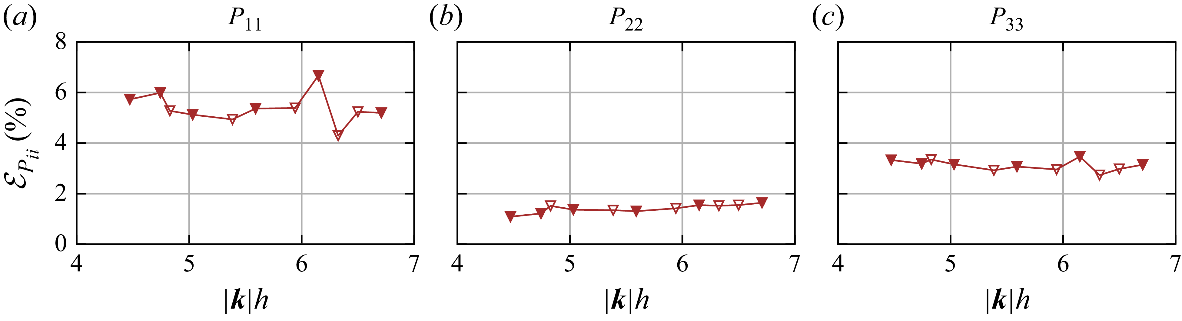
Figure 9 shows the prediction error of the neural operator model in the forcing spectra using the Cess eddy-viscosity profile, where the training scales are marked with filled triangles. It can be seen that the prediction error is within
 $8\,\%$
for the streamwise components,
 $2\,\%$
for the wall-normal components and
 $4\,\%$
for the spanwise components. Also, the prediction errors on unseen wavenumbers remain comparable to those at the training wavenumbers, indicating that the learned forcing model could be applied to different wavenumbers near the training scales. In addition, the Cess eddy viscosity and corresponding mean velocity are unseen in the training dataset, which indicates that the learned neural operator can be applied to unseen RANS models. The model generalisation across different wavenumbers and eddy-viscosity models in terms of the velocity statistics will be discussed in § 5.5.
Relative error
 $\mathcal{E}_{P_{ii}}$
between the neural operator-based predictions and the target stochastic forcing spectra in terms of (a)
 $P_{11}$
, (b)
 $P_{22}$
and (c)
 $P_{33}$
with
 $Re_\tau =180$
using the Cess model at different characteristic scales. The error is computed based on (5.1). The filled and hollow markers denote the training and testing scales, respectively.

Normalised frequency spectra of velocity (a–c)
 $\tilde {u}$
, (d–f)
 $\tilde {v}$
and (g–i)
 $\tilde {w}$
at the wavenumber
 $\boldsymbol{k}h=(2,4)$
with
 $Re_\tau =180$
. The results are shown for (a,d,g) DNS, (b,e,h) the learned and (c,f,i) white-noise (w.n.) predictions. The spectra are normalised such that their integral over frequency and wall-normal direction equals one. Solid and dashed black lines indicate isolines of DNS and resolvent predictions, respectively, and the red dashed line denotes the frequency
 $k_x U(y)$
. The red crosses indicate the peak location of the velocity spectra.

5.2. Prediction of velocity spectra
The proposed neural operator-based forcing model can provide accurate predictions in the velocity spectra. This is evident in figure 10, where the velocity spectra predicted by the learned model are compared against the DNS and the white-noise prediction at the wavenumber
 $\boldsymbol{k}h=(2,4)$
for channel flows at the Reynolds number
 $Re_\tau =180$
. Note that the Cess eddy-viscosity model is tuned for high-Reynolds-number flows (Cess Reference Cess1958), and its accuracy at low to moderate Reynolds numbers (e.g.
 $Re_\tau =180$
,
 $550$
) is not guaranteed (Morra et al. Reference Morra, Nogueira, Cavalieri and Henningson2021). In view of this, we employ the learned forcing model with the Cess eddy-viscosity profile, while equipping the white-noise forcing model with the DNS-derived eddy-viscosity profile that is considered the most accurate eddy viscosity for modelling Reynolds stresses of channel flows. This highlights the predictive performance of the proposed neural operator-based forcing, independent of the employed eddy-viscosity models. The velocity spectra are computed using (2.6) given the modelled forcing spectra
 $\boldsymbol{P}$
. The present velocity spectra are normalised by
 $ [\boldsymbol{S} ]$
to depict the spectral energy density distribution in the frequency
 $\omega$
and wall-normal position
 $y$
at specified wavenumbers. For a fixed wall-normal position, the spectral energy is concentrated within a narrow frequency band centred around the peak frequency
 $k_xU_c$
. In the channel flows, the convective velocity
 $U_c$
is close to the mean velocity
 $U$
in the buffer layer and above (as indicated by the red dashed line in figure 10), while remaining constant within the viscous sublayer (del Álamo & Jiménez Reference Hwang and Cossu2009). The wall-parallel velocity components have spectral peaks at
 $y^+\simeq 30\sim 40$
and the wall-normal velocity has spectral peaks near
 $y^+\simeq 70$
. It can be seen that the learned forcing model correctly captures the peak frequency and the peak wall-normal positions. In contrast, the white-noise stochastic forcing noticeably underestimates the peak frequency for the wall-parallel velocity components. Moreover, the white noise underestimates the peak positions of wall-parallel velocity spectra at
 $y^+\simeq 10{\sim}20$
and overestimates the peak position of wall-normal velocity spectra at
 $y^+\simeq 180$
, i.e. the channel centre. The isolines in figure 10 correspond to contour levels, evenly spaced at logarithmical intervals of
 $1\times 10^{-1}$
. The close agreement between the learned predictions and DNS results demonstrates that the neural operator-based forcing model accurately predicts both the frequency bandwidth and wall-normal energy distribution for each velocity component. In contrast, the white-noise forcing model overestimates the frequency bandwidth, resulting in inaccurate temporal dynamics. The predictions of the off-diagonal element
 $\langle \tilde {u}\tilde {v}^{{H}}\rangle$
by the learned model and the white-noise forcing are similar based on our numerical experiments, and hence, the plots are omitted here.
The learned forcing model can accurately predict the velocity frequency spectra across different wavenumbers. It is supported in figure 11, which presents the normalised spectra predicted by the learned forcing model at a spanwise wavenumber of
 $k_zh=4.5$
and scale ratios
 $\lambda _x/\lambda _z=9,3,2.5,2$
for flows of the Reynolds number
 $Re_\tau =180$
, with comparison to the DNS results. The frequency spectra are plotted at the peak wall-normal position indicated in figure 10. Figure 11(a) shows the streamwise velocity spectrum of the long streaky structure, with a spectral peak in the log-law region at
 $y^+\simeq 84$
. Figures 11(b)–11(d) show the spectra for the short and tall vortex packets, exhibiting the spectral peaks at
 $y^+\simeq 28,62$
and
 $73$
located in the buffer layer and log-law region. The frequency
 $k_x U$
is shown as black dashed lines in figure 11. It can be observed that the peak frequencies for all three velocity components closely match
 $k_xU$
, confirming that the convection velocity approximates the local mean velocity. The streamwise velocity exhibits the strongest spectral intensity across different scales among the three velocity components, which can be predicted by both forcing models. On the other hand, the velocity spectra decay rapidly away from the peak frequency. The learned forcing model accurately captures this decay behaviour, while the white-noise stochastic forcing provides spectral energy larger than the DNS results by orders of magnitude at frequencies away from the peak.
Normalised frequency spectra of the velocity components for flows of
 $Re_\tau =180$
in terms of
 $S_{11}$
,
 $S_{22}$
and
 $S_{33}$
with comparison between the DNS and the resolvent-based predictions with the learned and white-noise (w.n.) forcing models. The frequency spectra are shown at the peak wall-normal position. The wavenumber is set as
 $k_zh=4.5$
, and the arrow indicates the increasing scale ratios
 $\lambda _x/\lambda _z=2, 2.5, 3, 9$
. The black dashed line in each plot indicates the frequency corresponding to
 $k_xU$
.

5.3. Prediction of time scales
We examine the performance of the learned neural operator-based forcing model in capturing the temporal characteristics of the large-scale turbulent structures. The time correlation of velocity components can be obtained from the frequency spectra as
 \begin{equation} R(\boldsymbol{k},\tau ,y)=\int _{-\infty }^{\infty }\varPhi e^{\textrm{i}\omega \tau }{\textrm{d}}{\omega },\quad \varPhi =\frac {\langle \tilde {u}\tilde {u}^{{H}}\rangle }{\int _{-\infty }^{\infty }\langle \tilde {u}\tilde {u}^{{H}}\rangle {\textrm{d}}{\omega }} \text{,} \end{equation}
where
 $\tau$
denotes the temporal separation and
 $\varPhi$
is the conditional frequency spectrum. The conditional spectrum is the wavenumber–frequency spectrum normalised by the total energy at given wavenumbers. This normalisation ensures the spectrum has a unit integral over frequency, enabling quantitative comparisons of frequency distributions (Ganapathisubramani et al. Reference Ganapathisubramani, Hutchins, Monty, Chung and Marusic2012; Ali, Mellado & Wilczek Reference Ali, Mellado and Wilczek2023). The time correlation of the streamwise velocity is computed using (5.3), and the same calculation is applied for other velocity components. Figure 12 compares the magnitude
 $| R|$
of time correlation of the streamwise velocity at the wavenumber
 $\boldsymbol{k}h=(0.5,5)$
(long streaky structure) and
 $\boldsymbol{k}h=(2,4)$
(short and tall vortex packet) for
 $Re_\tau =180$
among the DNS, the learned predictions and the white-noise predictions. The time correlations are shown at three wall-normal positions, i.e.
 $y^+=11$
(buffer layer),
 $y^+=80$
(log-law region) and
 $y^+=180$
(channel centre). Figure 12(a–c) illustrates the time correlation for the long streaky structure. The DNS results reveal that the time correlation of this coherent structure decays most rapidly in the channel centre compared with the buffer layer and log-law region. Figure 12(d–f) illustrates the time correlation for the tall and short vortex packets. It can be seen that the time correlation in the buffer layer has the fastest decay rate, whereas those in the log layer and near the channel centre exhibit relatively slow decay. The learned forcing model accurately predicts the time correlation in good agreement with the DNS results across the present three wall-normal positions. In contrast, the white-noise-based predictions exhibit an abrupt drop at
 $\tau =0$
and fail to capture the correct decay behaviour at the three wall-normal locations. In general, the learned coloured-in-time forcing model can significantly improve the prediction of the time correlation compared with the white-noise forcing.
Time correlation of
 $\tilde {u}$
at wavenumbers (a–c)
 $\boldsymbol{k}h=(0.5,5)$
and (d–f)
 $\boldsymbol{k}h=(2,4)$
for
 $Re_\tau =180$
. The results are shown at wall-normal positions (a,d)
 $y^+=11$
in the buffer layer, (b,e)
 $y^+=80$
in the log-law region and (c,f)
 $y^+=180$
at the channel centre. The results of the DNS, the learned and the white-noise (w.n.) models are compared in each panel.

To further examine the temporal predictive performance of the learned forcing model, we compare the predicted Taylor time microscales with the DNS data. The Taylor time microscale can characterise the decay rate of time correlation near the temporal separation
 $\tau =0$
, which is defined as
 \begin{equation} \lambda _T=\left (-\frac {1}{2}\frac {\partial ^2| R|}{\partial \tau ^2}\bigg |_{\tau =0}\right )^{-1/2}. \end{equation}
It can be calculated using the first- and second-order conditional moments (Wu & He Reference Wu and He2021) of the frequency spectra as
 \begin{equation} \lambda _T(\boldsymbol{k},y)=\left [ \frac {1}{2}\int _{-\infty }^{\infty }\omega ^2\varPhi {\textrm{d}}{\omega }-\frac {1}{2}\left (\int _{-\infty }^{\infty }\omega \varPhi {\textrm{d}}{\omega }\right )^2 \right ]^{-1/2} {,} \end{equation}
where the conditional frequency spectrum
 $\varPhi$
is defined in (5.3). Figure 13 presents the Taylor time microscales of the velocity components at the wavenumber
 $\boldsymbol{k}h=(0.5,5)$
and
 $\boldsymbol{k}h=(2,4)$
for
 $Re_\tau =180$
. The long streaky structure at
 $\boldsymbol{k}h=(0.5,5)$
exhibits relatively large Taylor time microscales compared with the short and tall vortex structure at
 $\boldsymbol{k}h=(2,4)$
, particularly for the streamwise velocity component. Moreover, the Taylor time microscales at
 $\boldsymbol{k}h=(0.5,5)$
are nearly uniform across the channel height, indicating a consistent decorrelation process. In contrast, the flow structure at
 $\boldsymbol{k}h=(2,4)$
shows a slower temporal correlation decay near the channel centre and a faster decay close to the wall. It can be seen that the white-noise stochastic forcing leads to large predictive discrepancies in the Taylor time microscales from the DNS results. Note that the Taylor time microscales using the white-noise forcing are theoretically expected to be zero (Wu & He Reference Wu and He2021), while they can exhibit very small values due to the finite frequency range and resolution in numerical simulations. Compared with the white-noise forcing, the learned forcing model significantly improves the estimation of the Taylor time microscales across the entire channel height for all three velocity components.
Taylor time microscales of
 $\tilde {u}$
,
 $\tilde {v}$
and
 $\tilde {w}$
at wavenumber (a–c)
 $\boldsymbol{k}h=(0.5,5)$
and (d–f)
 $\boldsymbol{k}h=(2,4)$
with
 $Re_\tau =180$
. Results are shown for the DNS, the learned predictions and the white-noise (w.n.) predictions.

The proposed neural operator-based forcing model can also provide accurate predictions of the integral time scales. It is evidenced in figure 14, which presents the integral time scales of the velocity components at the wavenumber
 $\boldsymbol{k}h=(0.5,5)$
and
 $\boldsymbol{k}h=(2,4)$
for flows of the Reynolds number
 $Re_\tau =180$
. The integral time scales are defined as
 \begin{equation} \lambda _I(\boldsymbol{k},y)=\int _{0}^{\infty }\mid {R}(\boldsymbol{k},\tau ,y) \mid {\textrm{d}}{\tau } {.} \end{equation}
The DNS results reveal contrasting trends for the two flow structures. For the streaky structure at
 $\boldsymbol{k}h=(0.5,5)$
, the integral time scales reach their maximum near the wall and decrease toward the channel centre, as shown in figure 14(a–c). In contrast, the short and tall vortex packets at
 $\boldsymbol{k}h=(2,4)$
display the opposite pattern, with integral time scales peaking at the channel centre and diminishing toward the walls, as shown in figure 14(d– f). The white-noise forcing can yield similar trends, while the predicted time scales deviate substantially from the DNS results, showing its difficulty in accurately capturing the decay of the time-correlation function over temporal separation. In contrast, the learned forcing model significantly improves the predictive accuracy of the integral time scales across the entire channel height for all three velocity components, closely aligning with the DNS results.
Integral time scales of
 $\tilde {u}$
,
 $\tilde {v}$
and
 $\tilde {w}$
at wavenumber (a–c)
 $\boldsymbol{k}h=(0.5,5)$
and (d–f)
 $\boldsymbol{k}h=(2,4)$
for
 $Re_\tau =180$
. Results are shown for the DNS, the learned predictions and the white-noise (w.n.) predictions.

5.4. Stochastic forcing projections
The projection of the learned forcing onto the resolvent mode is examined here to reveal the energy amplification in the channel flows. Specifically, the resolvent operator
 $\boldsymbol{R}$
can be decomposed with singular value decomposition (SVD) as
 \begin{equation} \boldsymbol{R}=\sum _{i=1}^{3N_y} \sigma _i\boldsymbol{\psi }_i\boldsymbol{\phi }_i^{{H}}. \end{equation}
The singular values
 $\sigma _i$
are real, positive scalars arranged in decreasing order
 $(\sigma _1\geqslant \sigma _2\geqslant {\cdots} )$
. The left- and right-singular vectors, i.e.
 $\boldsymbol{\psi }_i$
and
 $\boldsymbol{\phi }_i$
, form output and input bases, respectively, satisfying the orthogonality
 $\boldsymbol{\psi }_i^{{H}} \boldsymbol{\psi }_j=\delta _{ij}$
and
 $\boldsymbol{\phi }_i^{{H}}\boldsymbol{\phi }_i=\delta _{ij}$
, with
 $\delta _{ij}$
being the Kronecker delta. With the SVD, the input–output relation in (2.6) can be expressed through resolvent output modes and stochastic forcing projections onto resolvent input modes (Morra et al. Reference Morra, Nogueira, Cavalieri and Henningson2021), i.e.
 \begin{equation} \boldsymbol{S}=\sum _{i=1}^{3N_y}\lambda _i^2 \boldsymbol{\psi }_i\boldsymbol{\psi }_i^{{H}},\quad \lambda _i^2=\sigma _i^2\boldsymbol{\phi }_i^{{H}} \boldsymbol{P}\boldsymbol{\phi }_i, \end{equation}
where
 $\lambda _i$
represents the projection of stochastic forcing onto the resolvent input bases, amplified by corresponding singular values
 $\sigma _i$
. This can be interpreted as the
 $i$
th modal energy gain from stochastic forcing to the velocity field. For the white-in-time stochastic forcing, where the spectrum
 $\boldsymbol{P}$
becomes an scalar matrix, the modal energy gain reduces to the singular value of the resolvent operator normalised by kinetic energy. For the DNS results, the energy gain can be derived by projecting the velocity cross-spectra
 $\boldsymbol{S}^{\textit{(DNS)}}$
onto the resolvent output bases as
 \begin{equation} \lambda _i^2=\boldsymbol{\psi }_i^{{H}}\boldsymbol{S}^{\textit{(DNS)}}\boldsymbol{\psi }_i. \end{equation}
Given that the resolvent modes in channel flows appear in even–odd pairs that share nearly identical singular values (Moarref et al. Reference Moarref, Sharma, Tropp and McKeon2013), we present the energy gains of the first and third resolvent modes at wavenumbers
 $\boldsymbol{k}h=(0.5,5)$
and
 $\boldsymbol{k}h=(2,4)$
for
 $Re_\tau =180$
in figure 15. Both the energy gains peak near the frequency
 $k_x U_{{m}}$
, corresponding to a wave speed approximately matching
 $U_{{m}}$
, and decay rapidly away from the peak frequency. The learned forcing and the white-noise forcing both correctly predict the peak frequency. However, the white-noise forcing produces energy gains orders of magnitude larger than the DNS away from the peak due to the uniform forcing amplitudes across all frequencies. In contrast, the learned forcing shows much closer agreement with the DNS in the overall energy-gain distribution. The white-noise results also show that the peak singular value of the third resolvent mode is only about 10 % of that of the first mode, while away from the peak, the singular value becomes comparable to that of the first mode. This dominance of the first resolvent mode near the peak frequency, where turbulence is active, also highlights the low-rank nature of the resolvent operator (McKeon Reference McKeon2017).
Note that for the wavenumber
 $\boldsymbol{k}h = (2,4)$
, the learned predictions yield higher energy gains than the DNS results at frequencies far above the peak. This is likely attributed to spatial decorrelation in the wall-normal direction and forcing componentwise decorrelation, which reduces the effectiveness of the forcing projection.
Normalised energy gain of the first and third resolvent modes at wavenumber (a)
 $\boldsymbol{k}h=(0.5,5)$
and (b)
 $\boldsymbol{k}h=(2,4)$
with
 $Re_\tau =180$
using the Cess model. Results are shown for the DNS, the learned predictions and the white-noise (w.n.) predictions.

5.5. Generalisation across wavenumbers and eddy-viscosity models
In the above subsections, we demonstrate the predictive ability of the learned forcing model at the wavenumbers
 $\boldsymbol{k}h=(0.5,5)$
and
 $\boldsymbol{k}h=(2,4)$
, using only the Cess model for flows of Reynolds number
 $Re_\tau =180$
. Here, we evaluate the performance for different wavenumbers and RANS models in terms of velocity frequency spectra and time-scale predictions for all three velocity components. The prediction error for the velocity frequency spectra, the Taylor time microscales and the integral time scales are evaluated against DNS results using
 \begin{align} \mathcal{E}_{S_{ii}}&=\int _{-\infty }^{\infty }\iint _{-h}^{h} \left | \frac {S_{ii}}{\left [\boldsymbol{S}\right ]}- \frac {S_{ii}^{\textit{(DNS)}}}{\left [\boldsymbol{S}^{\textit{(DNS)}}\right ]} \right |\delta (y-y') {\textrm{d}}{y}{\textrm{d}}{y'}{\textrm{d}}{\omega }, \end{align}
 \begin{align} \mathcal{E}_T&=\frac { \int _{-h}^{h}\big | \lambda _T-\lambda _T^{\textit{(DNS)}}\big |{\textrm{d}}{y} }{ \int _{-h}^{h}\lambda _T^{\textit{(DNS)}}{\textrm{d}}{y} }, \end{align}
 \begin{align} \mathcal{E}_I&=\frac { \int _{-h}^{h}\big | \lambda _I-\lambda _I^{\textit{(DNS)}}\big |{\textrm{d}}{y} }{ \int _{-h}^{h}\lambda _I^{\textit{(DNS)}}{\textrm{d}}{y} }. \end{align}
The frequency spectra of each velocity component are normalised by the same scaling factor, i.e. the total kinetic energy
 $ [\boldsymbol{S} ]$
from all three velocity components, ensuring that the error metric can be compared consistently across components. The error metric
 $\mathcal{E}_{S_{ii}}$
represents the mean difference in normalised velocity spectra, quantifying the discrepancy of model predictions from the DNS results across frequencies and wall-normal positions.
Figure 16(a–c) presents the error metrics of the frequency spectra
 $\langle \tilde {u}_i\tilde {u}_i^{\textit{H}}\rangle$
for the three velocity components. The learned forcing model achieves a
 $50\,\%$
reduction in velocity prediction error compared with the white-noise stochastic forcing across the scales examined. The streamwise velocity spectra exhibit the largest discrepancies with the white-noise forcing, producing approximately
 $50\,\%$
error, while the learned forcing maintains errors around
 $20\,\%$
. The wall-normal and spanwise velocity components show lower error levels around
 $10\,\%$
and
 $20\,\%$
, respectively, likely due to their lower energy intensity compared with the streamwise component. Nevertheless, the learned forcing can achieve further improvement, reducing the predictive errors to
 $5\,\%$
and
 $10\,\%$
, respectively. Different RANS models exhibit consistent error levels for the wall-normal and spanwise velocities. Although the three RANS models produce relatively different prediction errors for the streamwise velocity spectra, they demonstrate significant improvement over white-noise forcing predictions across the characteristic scales. Figure 16(d–f) shows the error metrics for the Taylor time microscales
 $\lambda _T$
for each velocity component. The learned forcing model, using different RANS-provided eddy viscosities, significantly reduces prediction errors compared with white-noise forcing. As discussed in § 5.3, the white-in-time stochastic forcing fails to capture the Taylor time microscales
 $\lambda _T$
, yielding prediction errors larger than
 $90\,\%$
. In contrast, the learned coloured-in-time forcing reduces the prediction errors to approximately
 $20\,\%$
for wall-parallel velocity components and below
 $10\,\%$
for the wall-normal velocity at high wavenumbers. Furthermore, the predictive accuracy remains consistent across the three RANS models. Figure 16(g–i) displays the error metrics for the integral time scales
 $\lambda _I$
across each velocity component. Notably, the white-noise stochastic forcing performs better for integral time scales than for the Taylor time microscales, particularly for the streamwise velocity at scales of a long streak structure, e.g.
 $|\boldsymbol{k}|h \approx 4.5$
. Nevertheless, at the scales of short and tall vortex packet structures, e.g.
 $|\boldsymbol{k}|h \approx 6.7$
, the white-noise forcing still leads to large error levels. Compared with the white-noise forcing, the learned model yields significantly lower prediction errors in
 $\lambda _I$
. The prediction error of integral time scales remains consistent below
 $10\,\%$
for each velocity component and across different RANS models. Also, it is observed that the distribution of velocity spectra errors over wavenumber magnitude does not follow a consistent trend with that of the characteristic time scales. The error metrics in figure 16 reveal that the different RANS models produce similar error levels when integrated with the learned forcing model. This demonstrates that the learned model can accurately predict the time-correlation functions regardless of the used RANS model.
Error metrics for (a–c) velocity frequency spectra
 $\mathcal{E}_{S_{ii}}$
, (d–f) Taylor time microscales
 $\mathcal{E}_T$
and (g–i) integral time scales
 $\mathcal{E}_I$
with
 $Re_\tau =180$
, at different characteristic scales. Results are shown for (a,d,g)
 $\tilde {u}$
, (b,e,h)
 $\tilde {v}$
and (c,f,i)
 $\tilde {w}$
. The prediction errors of the learned and the white-noise (w.n.) forcings are evaluated using eddy viscosities from the DNS (squares), Cess (down triangles), S-A (circles) and
 $k$
-
 $\omega$
models (up triangles).

5.6. Generalisation at the Reynolds number
 $Re_\tau =550$

Finally, we show the generalisation capability of the learned forcing model for channel flows with
 $Re_\tau =550$
, at the characteristic scales indicated in figure 4. Figure 17 presents normalised velocity frequency spectra at the wavenumbers
 $\boldsymbol{k}h=(0.5,5)$
and
 $\boldsymbol{k}h=(3,6)$
with comparison among the learned prediction, the white-noise prediction and the DNS results. The spectra are evaluated at the peak wall-normal positions of the streamwise velocity spectra, i.e.
 $y^+\simeq 397$
for
 $\boldsymbol{k}h=(0.5,5)$
and
 $y^+\simeq 233$
for
 $\boldsymbol{k}h=(3,6)$
, both within the log-law region. The learned predictions are based on the Cess model, while the white-noise predictions use the DNS-derived eddy viscosity and mean velocity. It can be observed that both the learned and white-noise predictions correctly capture the peak frequency. However, the white-noise forcing significantly underestimates the spectral decay rate, exhibiting spectral energy larger than the DNS results by orders of magnitude away from the peak frequency. This leads to a broadened frequency bandwidth. In contrast, the learned forcing produces the accurate spectral decay across the three velocity components at both wavenumbers.
Normalised frequency spectra of the velocity components at wavenumber (a–c)
 $i = 1,i = 2, i = 3, \boldsymbol{k}h=(0.5,5)$
and (d–f)
 $i = 1,i = 2,i = 3, \boldsymbol{k}h=(3,6)$
for channel flows of
 $Re_\tau =550$
in terms of
 $S_{11}$
,
 $S_{22}$
and
 $S_{33}$
with comparison among the learned prediction, the white-noise (w.n.) prediction and the DNS results. The frequency spectra are shown at the peak wall-normal position. The black dashed line in each plot indicates the frequency of
 $k_xU$
.

Figure 18 shows the Taylor time microscales at wavenumbers
 $\boldsymbol{k}h=(0.5,5)$
and
 $\boldsymbol{k}h=(3,6)$
for channel flows of Reynolds number
 $Re_\tau =550$
. Similar to the flow at
 $Re_\tau =180$
as shown in figure 13, the long streaky structure at
 $\boldsymbol{k}h=(0.5,5)$
exhibits relatively uniform Taylor time microscales, which are larger than those of the short and tall vortex packet at
 $\boldsymbol{k}h=(3,6)$
. The vortex packet has the largest Taylor time microscale in the channel centre, which decreases toward the walls. For the streaky structure at
 $\boldsymbol{k}h=(0.5,5)$
, the learned forcing also shows noticeable discrepancies compared with the DNS results, while it performs significantly better than the white-noise forcing. For the short and tall vortex packets at
 $\boldsymbol{k}h=(3,6)$
, the learned forcing accurately predicts the Taylor time microscales, closely matching the DNS results.
Taylor time microscales of
 $\tilde {u}$
,
 $\tilde {v}$
and
 $\tilde {w}$
at wavenumber (a–c)
 $\boldsymbol{k}h=(0.5,5)$
and (d–f)
 $\boldsymbol{k}h=(3,6)$
with
 $Re_\tau =550$
. Results are shown for the DNS, the learned predictions and the white-noise (w.n.) predictions.

Figure 19 presents the integral time scales at the same wavenumber and Reynolds number as in figure 18. The streaky structure at
 $\boldsymbol{k}h=(0.5,5)$
exhibits significantly larger integral time scales compared with the short and tall vortex packets. Similar to the case of
 $Re_\tau =180$
, the short and tall vortex packets have peak integral time scales in the channel centre that decrease toward the walls. The white-noise forcing results in significant deviations from the DNS data at both wavenumbers. In contrast, the learned predictions can achieve remarkable agreement with the DNS results, particularly for the short and tall vortex packets at
 $\boldsymbol{k}h=(3,6)$
.
Integral time scales of
 $\tilde {u}$
,
 $\tilde {v}$
and
 $\tilde {w}$
at wavenumber (a–c)
 $\boldsymbol{k}h=(0.5,5)$
and (d–f)
 $\boldsymbol{k}h=(3,6)$
with
 $Re_\tau =550$
. Results are shown for the DNS, the learned predictions and the white-noise (w.n.) predictions.

Figure 20 presents the error metrics for the frequency spectra
 $\mathcal{E}_{S_{ii}}$
, Taylor time microscales
 $\mathcal{E}_T$
and integral time scales
 $\mathcal{E}_I$
across each velocity component at different characteristic scales for channel flows of
 $Re_\tau =550$
. The learned forcing reduces the prediction errors of velocity spectra by nearly half compared with white-noise forcing. Specifically, the prediction errors are decreased from (
 $50\,\%$
,
 $10\,\%$
,
 $20\,\%$
) to (
 $20\,\%$
,
 $5\,\%$
,
 $10\,\%$
) for streamwise, wall-normal and spanwise components, respectively. For Taylor time microscales, the learned forcing provides the prediction errors below
 $20\,\%$
for each velocity component, showing significant improvements over the white-noise forcing. Similarly, the prediction error of the integral time scale remains below
 $20\,\%$
. The white-noise forcing can make relatively better predictions for the integral time-scale prediction at the wavenumbers
 $|\boldsymbol{k}|h \lt 5$
while leading to discrepancy near
 $60\,\%$
at the wavenumber
 $|\boldsymbol{k}|h \approx 6.7$
. In contrast, the learned forcing model can provide consistently improved predictions across the different wavenumbers. In figure 20(a) it can be observed that the streamwise velocity spectra at wavenumber
 $\boldsymbol{k}h=(0.5,5)$
by the learned forcing exhibit slightly larger prediction errors using the
 $k$
–
 $\omega$
RANS model. This discrepancy may stem from substantial differences in the eddy-viscosity profile provided by the
 $k$
–
 $\omega$
model compared with other models at Reynolds number
 $Re_\tau =550$
, as shown in Appendix B. The generalisation capability of the learned model can be attributed to the interpolation ability of DeepONet, as the eddy-viscosity profiles for
 $Re_\tau =550$
largely fall within the range of the sampled profiles for
 $Re_\tau =180$
, as illustrated in figure 5. The predictive performance of the learned model could be further validated at higher Reynolds numbers, such as
 $Re_\tau =5200$
, while it faces difficulties in data availability due to prohibitive storage requirements for temporal Fourier analysis at this Reynolds number regime.
Error metrics for (a–c) velocity frequency spectra
 $\mathcal{E}_{S_{ii}}$
, (d–f) Taylor time microscales
 $\mathcal{E}_T$
and (g–i) integral time scales
 $\mathcal{E}_I$
with
 $Re_\tau =550$
, evaluated at different characteristic scales. Results are shown for (a–d–g)
 $\tilde {u}$
, (b–e–h)
 $\tilde {w}$
and (c–f–i)
 $\tilde {w}$
. The prediction errors of the learned and the white-noise (w.n.) forcings are evaluated using eddy viscosities from the DNS, Cess, S-A and
 $k$
–
 $\omega$
models.

6. Conclusion
In this work we propose using the neural operator-based coloured-in-time forcing for predicting the space–time properties of large-scale flow structures based on the RANS-predicted eddy viscosity and mean velocity. It is achieved by combining the eddy-viscosity enhanced resolvent operator and the neural operator-based stochastic forcing model. Specifically, the neural operator based on the DeepONet architecture is used to construct the mapping from the eddy viscosity and mean velocity to the coloured-in-time stochastic forcing spectra. Furthermore, the resolvent operator is used to map the obtained stochastic forcing spectra to the space–time velocity statistics. In doing so, the neural operator-enhanced resolvent model can accurately predict the velocity statistics without requiring available data, which enables the learned stochastic forcing model to be applied in different flow conditions. Also, the DeepONet-based model is flexible in evaluating arbitrary domain locations of the stochastic forcing, allowing for predictions of velocity spectra at different spatial–temporal scales. Besides, the neural operator-based forcing model can be well generalised to different RANS-provided eddy viscosity and mean velocity profiles.
The neural operator-based stochastic forcing is first trained based on the DNS data of the channel flow at
 $Re_\tau =180$
. We show that the learned neural operator model can accurately predict the stochastic forcing spectra and the velocity response of large-scale flow structures. Particularly, the learned model can significantly improve the prediction of time correlation and the characteristic time scales compared with the conventional white-noise forcing. Also, we show that the neural operator-based model can be coupled with different RANS models, providing consistent predictions in velocity statistics. Furthermore, the proposed neural operator can be applied to the channel flow at
 $Re_\tau =550$
, making accurate predictions in the space–time characteristics of large-scale flow structures.
In the present work the forcing model is learned for large-scale structures of channel flows, which may have issues when applied to predict the small-scale flow statistics. However, we note that the proposed method can be used to train specific neural operator models for small-scale flow structures with inner-scale-based normalisation. Also, the learned model in the present work has difficulties to be generalised to different configurations from channel flows. Specific stochastic forcing models could be learned from high-fidelity data in other flow scenarios, such as jet flows, using the neural operator-based method. In addition, the normal-to-wall correlation and cross-component correlation of the stochastic forcing are neglected in the present work, which can be further involved in the neural operator model in future work. Besides, the present work focuses on the stochastic forcing model in the eddy-viscosity enhanced resolvent framework, which compensates the RANS model errors in the stochastic forcing. It would be worthy of further investigation to improve both the RANS model and the nonlinear forcing model with the data-driven approaches, particularly in complex flow, e.g. with separation, which has significant RANS model errors. In doing so, the RANS model can provide the proper eddy viscosity and accurate mean velocity to improve the resolvent-based linear operator. The forcing model further yields the coloured-in-time input excitation, leading to accurate velocity spectra.
Funding
This work is supported by NSFC Excellence Research Group Program for ‘Multiscale Problems in Nonlinear Mechanics’ (No. 12588201). XLZ also acknowledges support from the Young Elite Scientists Sponsorship Program by CAST (No. 2022QNRC001) and the CAS Project for Young Scientists in Basic Research (YSBR-087).
Declaration of interests
The authors report no conflict of interest.
Appendix A. Resolvent operators
The operators in the evolution (2.3) are defined as
 \begin{equation} \boldsymbol{A}_{\nu _t}=\begin{bmatrix} \varDelta ^{-1}\mathcal{L}_{\textit{OS}} & 0 \\ -{\textrm{i}} k_z U^{\prime} & \mathcal{L}_{\textit{SQ}} \end{bmatrix},\quad \boldsymbol{B}=\begin{bmatrix} -{\textrm{i}} k_x\varDelta ^{-1}{\partial _y} & -k^2\varDelta ^{-1} & -{\textrm{i}} k_z\varDelta ^{-1}{\partial _y} \\ {\textrm{i}} k_z & 0 & -{\textrm{i}} k_x \end{bmatrix}, \end{equation}
where
 $\mathcal{L}_{\textit{OS}}$
is the generalised Orr–Sommerfeld and
 $\mathcal{L}_{\textit{SQ}}$
is the Squire operator (Cossu et al. Reference Cossu, Pujals and Depardon2009), which are defined as
 \begin{align} \mathcal{L}_{\textit{OS}}&=-{\textrm{i}} k_x (U\!\Delta -U^{\prime \prime})+ (\nu +\nu _t)\varDelta ^2+2\nu ^{\prime}_t\Delta \partial _y+\nu ^{\prime \prime}_t (\partial _{yy}+k^2), \end{align}
 \begin{align} \mathcal{L}_{\textit{SQ}}&=-{\textrm{i}} k_x U + (\nu +\nu _t)\varDelta +\nu ^{\prime}_t\partial _y. \end{align}
Here the prime notation denotes differentiation with respect to the wall-normal coordinate
 $y$
. Additionally,
 $k^2=k_x^2+k_z^2$
and the Laplacian in wavenumber space is
 $\varDelta =\partial _{yy}-k^2$
. All operators are discretised via a spectral collocation method with Chebyshev-based differentiation matrices. The transformation matrices relating velocity vector
 $\tilde {\boldsymbol{u}}$
and state vector
 $\tilde {\boldsymbol{q}}$
are
 \begin{equation} \boldsymbol{C}=\frac {1}{k^2}\begin{bmatrix} {\textrm{i}} k_x\partial _y & -{\textrm{i}} k_z \\ k^2 & 0 \\ {\textrm{i}} k_z \partial _y & {\textrm{i}} k_x \end{bmatrix},\quad \boldsymbol{D}=\begin{bmatrix} 0 & 1 & 0\\ {\textrm{i}} k_z & 0 & -{\textrm{i}} k_x \end{bmatrix}. \end{equation}
Appendix B. The RANS models
The RANS equations in turbulent channel flow for the zero-equation Cess model, the one-equation S-A model and the two-equation
 $k$
–
 $\omega$
model are presented. In channel flows, the RANS momentum equation with the eddy-viscosity-based turbulence models can be written as
 \begin{equation} -\frac {u_\tau ^2}{h}=\frac {{\textrm{d}}{}}{{\textrm{d}}{y}}\left [ (\nu +\nu _t) \frac {{\textrm{d}}{U}}{{\textrm{d}}{y}}\right ], \end{equation}
subject to the boundary condition
 $U(\pm h)=0$
, where
 $u_\tau$
is the friction velocity.
The zero-equation Cess model (Cess Reference Cess1958; Reynolds & Tiederman Reference Reynolds and Tiederman1967) provides the eddy viscosity as a function of wall-normal position, i.e.
 \begin{equation} \nu _t(y)=\frac {\nu }{2}\sqrt {1+\frac {\kappa ^2 Re_\tau ^2}{9} \left(1-\frac {y^2}{h^2} \right)^2\left (1+\frac {2y^2}{h^2}\right )^2\left (1-e^{-y^+/A}\right )^2}-\frac {\nu }{2}, \end{equation}
where
 $A^+=25.4$
,
 $\kappa =0.426$
is the Kármán constant and
 $y^+=Re_\tau (1-|y/h|)$
is the distance from the nearest wall measured in viscous length scales. The Cess model offers an explicit formula, enabling a direct solution of eddy viscosity in channel flows.
The S-A model (Spalart & Allmaras Reference Spalart and Allmaras1992) provides the eddy viscosity by
 \begin{align} \nu _t &=\hat {\nu }f_{v1}, \end{align}
 \begin{align} 0 =c_{b1} (1-f_{t2})\hat {S}\hat {\nu } \!-\! \Big (c_{w1}f_w-\frac {c_{b1}}{\kappa ^2}f_{t2}\Big )\left (\frac {\hat {\nu }}{d}\right )^2 & \!+\! \frac {1}{\sigma }\left [\frac {\partial }{\partial y}\left ((\nu +\hat {\nu })\frac {\partial \hat {\nu }}{\partial y}\right )+c_{b2}\left (\frac {\partial \hat {\nu }}{\partial y}\right )^2\right ] , \end{align}
subject to boundary conditions
 $\hat {\nu }(\pm h)=0$
. Auxiliary functions and constants are
 \begin{align} f_{v1} &=\frac {\chi ^3}{\chi ^3+c_{v1}^3},\quad f_{v2}=1-\frac {\chi }{1+\chi f_{v1}},\quad f_{t2}=c_{t3}\exp \big (-c_{t4}\chi ^2\big ),\quad \chi =\frac {\hat {\nu }}{\nu }, \end{align}
 \begin{align} \hat {S} &=|\partial _y U|+\frac {\hat {\nu }}{\kappa ^2 d^2}f_{v2},\quad f_w=g\left (\frac {1+c_{w3}^6}{g^6+c_{w3}^6}\right )^{1/6},\quad g=r+c_{w2}\big (r^6-r\big ), \end{align}
 \begin{align} r &=\min \left [\frac {\hat {\nu }}{\hat {S}\kappa ^2 d^2},10\right ],\quad \sigma =2/3,\, \kappa =0.41,\, c_{v1}=7.1, \end{align}
 \begin{align} c_{b1} &=0.1355,\, c_{b2}=0.622,\,c_{w1}=3.239,\, c_{w2}=0.3,\, c_{w3}=2,\, \, c_{t3}=1.2,\, c_{t4}=1/2. \end{align}
The
 $k$
–
 $\omega$
model (Wilcox Reference Wilcox1998, Reference Wilcox2008) specifies the eddy viscosity by
 \begin{align} \nu _t &={k}/{\omega }, \end{align}
 \begin{align} 0 & =\nu _t\!\left (\partial _y U\right )^2-\beta ^*\omega k+\partial _y\left [(\nu +\sigma ^*\nu _t)\partial _y k\right ], \end{align}
 \begin{align} 0 &=\gamma\! \left (\partial _y U\right )^2-\beta \omega ^2+\partial _y\left [(\nu +\sigma \nu _t)\partial _y\omega \right ], \end{align}
subject to boundary conditions
 $k(\pm h)=0,\lim _{d\to 0}\omega =6\nu /(\beta d^2)$
, where
 $d$
is the distance to the nearest wall. The model constants are
 \begin{equation} \beta ^*=9/100,\quad \beta =3/40,\quad \sigma ^*=1/2,\quad \sigma =1/2,\quad \gamma =5/9. \end{equation}
The eddy viscosities and mean profiles obtained from the Cess, S-A and
 $k$
–
 $\omega$
models are compared against DNS results in figure 21.
Comparison of (a,c) eddy viscosity and (b,d) mean velocity profiles between RANS models and DNS for turbulent channel flow of (a,b)
 $Re_\tau =180$
and (c,d)
 $Re_\tau =550$
.

The RANS equations coupled with the S-A and
 $k$
–
 $\omega$
models yield a one-dimensional system of nonlinear ordinary differential equations. The numerical solution is obtained via Picard iteration (Hairer, Nørsett & Wanner Reference Hairer, Nørsett and Wanner1993), with the diffusion terms treated implicitly. To enhance robustness, all variables are updated using an under-relaxation scheme during the iterative process. For spatial discretisation in the wall-normal direction (
 $y$
), Chebyshev collocation points are utilised, identical to those employed in DNS. The derivatives are computed via Chebyshev polynomial approximation (Orszag Reference Orszag1971a
), ensuring spectral accuracy. The iteration process is terminated when the residual converges to machine precision.
Appendix C. DNS data analysis
In the DNS, flow snapshots are recorded after the flow reaches a statistically steady state. The time Fourier transformation is performed using Welch’s method with a Hann window and
 $75\,\%$
overlap. A
 $\sqrt {8/3}$
correction factor is applied to the frequency modes to ensure energy conservation. The Hann window spans
 $N$
snapshots, providing a frequency resolution of
 $\Delta \omega =2\pi /(N\Delta t_{{sample}})$
, with the frequency range extending from
 $-({N}/{2}) \Delta \omega$
to
 $({N}/{2}-1)\Delta \omega$
. The frequency range must be adequately wide to fully encompass the spectral energy of the flow variables, such that their spectra diminish to negligible levels at the range boundaries for all relevant wavenumbers and wall-normal positions. For both the
 $Re_\tau =180$
and
 $Re_\tau =550$
cases, flow snapshots are sampled at uniform time intervals of
 $\Delta t_{{sample}}={5\times 10^{-2}}h/U_{{m}}$
. A Hann window of length
 $N={1024}$
snapshots is applied, corresponding to a time duration of
 $T=51.2 h/U_{{m}}$
. A total of
 $10\,001$
snapshots and
 $5400$
snapshots are collected for the
 $Re_\tau =180$
case and the
 $Re_\tau =550$
case, respectively.
Error metrics of the streamwise velocity spectra at wavenumber
 $\boldsymbol{k}h=(2,4)$
for
 $Re_\tau =180$
. (a) Frequency spectra at the peak frequency; (b) error of spectra at peak frequency; (c) wall-normal integrated error metrics; (d) cumulative error metrics evaluated over frequency ranges.

Appendix D. Discussion on error metrics
This section examines the error metrics of the streamwise velocity spectra, using the wavenumber
 $\boldsymbol{k}h=(2,4)$
for
 $Re_\tau =180$
. The predictive error of the velocity spectra is around
 $20\,\%$
with the learned model as shown in figure 16(a). The large quantified errors are mainly due to discrepancies in the wall-normal distribution, which is supported by figure 22. Figure 22(a) presents the velocity spectra at the peak frequency, with the horizontal dashed lines denoting their corresponding averaged values along the wall-normal direction. The learned model closely agrees with the DNS in the averaged value, with the difference being about 0.043, as indicated by the gap between the dashed lines. However, the error metric using (5.10a
) quantifies predictive discrepancies in the wall-normal distribution rather than wall-normal averaged values. Given this, figure 22(b) examines the absolute errors of resolvent predictions at the peak frequency compared with the DNS, along with their wall-normal mean errors defined as
 \begin{equation} \frac {1}{2h}\int _{-h}^{h}\left | \langle \tilde {u}\tilde {u}^{{H}}\rangle -\langle \tilde {u}\tilde {u}^{{H}}\rangle ^{\textit{(DNS)}}\right |{\textrm{d}}{y}. \end{equation}
The mean error of the learned prediction is about 0.13 (red dashed line), which is considerably larger than the difference in wall-normal averaged spectra shown in figure 22(a). This indicates that the error mainly lies in deviations of the wall-normal distribution, though the total kinetic energy can be accurately reproduced. Furthermore, figure 22(c) presents the wall-normal integrated errors across frequencies, which indicates non-negligible errors near the peak frequency. Figure 22(d) shows the cumulative error integral over the frequency interval
 $ [-\bar {\omega },\bar {\omega } ]$
with
 $\bar {\omega }\geqslant 0$
, defined as
 \begin{equation} \int _{-\bar {\omega }}^{\bar {\omega }}\int _{-h}^{h}\left | \langle \tilde {u}\tilde {u}^{{H}}\rangle -\langle \tilde {u}\tilde {u}^{{H}}\rangle ^{\textit{(DNS)}}\right |{\textrm{d}}{y}{\textrm{d}}{\omega }, \end{equation}
which increases monotonically from zero at
 $\bar {\omega }=0$
. Both the learned and white-noise forcings exhibit rapid error growth before converging near
 $\bar {\omega } \sim 2k_xU_{{m}}$
. The white-noise forcing yields substantially larger errors (40 %) than the learned model (17 %), particularly for
 $\bar {\omega } \geqslant 2k_xU_{{m}}$
. The converged error levels in figure 22(d) are consistent with those presented in figure 16.