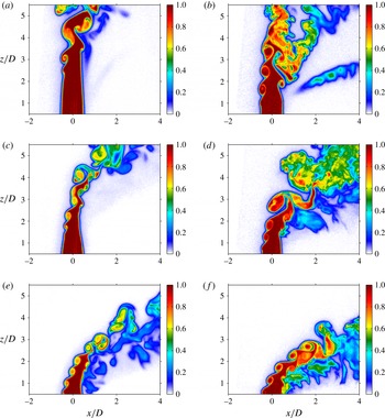
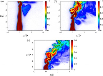
1. Introduction
Jets injected transversely into cross-flow have a wide range of applications in thermal-fluid systems, particularly those which require high rates of efficient mixing and energy release (Margason Reference Margason1993; Karagozian Reference Karagozian2010). The jet in cross-flow (JICF) studied experimentally in this paper focuses on gaseous mixtures of helium and nitrogen injected from a round orifice perpendicularly into a cross-flow of air, with an emphasis on the quantification of injectant–cross-flow molecular mixing for a range of flow conditions. Among the important flow-field parameters governing the evolution of the JICF are the jet-to-cross-flow velocity ratio,
 $R\equiv U_{j}/U_{\infty }$
, the jet-to-cross-flow density ratio,
 $S\equiv {\it\rho}_{j}/{\it\rho}_{\infty }$
, the jet-to-cross-flow momentum flux ratio,
 $J\equiv SR^{2}$
, and the jet Reynolds number,
 $Re_{j}\equiv U_{j}D/{\it\nu}_{j}$
, based on the jet exit diameter
 $D$
, the bulk jet velocity
 $U_{j}$
and the kinematic viscosity
 ${\it\nu}_{j}$
of the jet fluid.
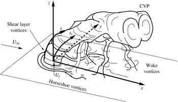
Schematic of the transverse jet, introduced flush with respect to the injection wall, including relevant vortical structures and orientation of coordinate axes. Adapted from Fric & Roshko (Reference Fric and Roshko1994).

The deceptively simple set-up of the jet in cross-flow creates a highly complex set of vortical systems, as shown for flush, perpendicular injection in figure 1. The appearance and relative strength of these vortical structures depends on the flow-field conditions. For instance, horseshoe vortices that wrap around the jet column have been shown to form for a wide range of flow conditions. These horseshoe vortices become unsteady at velocity ratios
 $R$
of 2 and 4, and at jet Reynolds numbers above approximately 2500 (Kelso & Smits Reference Kelso and Smits1995). Transient wake vortices, which are known to draw wall boundary layer fluid into the jet itself, have also been shown to vary in strength and coherency depending on velocity ratio (Fric & Roshko Reference Fric and Roshko1994; Smith & Mungal Reference Smith and Mungal1998). While it is likely that these vortical systems affect the mixing efficiency of the flow field to some degree, it is widely believed that enhanced mixing rates associated with the JICF, as compared to the free jet, can be attributed primarily to the formation and evolution of the counter-rotating vortex pair (CVP) which dominates the jet cross-section (Kamotani & Greber Reference Kamotani and Greber1972; Moussa, Trischka & Eskinazi Reference Moussa, Trischka and Eskinazi1977; Broadwell & Breidenthal Reference Broadwell and Breidenthal1984; Karagozian Reference Karagozian1986; Smith & Mungal Reference Smith and Mungal1998). The CVP has been shown to form in the near-field region of the jet, within a few diameters of injection, and is associated with the evolution and reorientation of vorticity in the shear layer (Kelso, Lim & Perry Reference Kelso, Lim and Perry1996; Cortelezzi & Karagozian Reference Cortelezzi and Karagozian2001) as well as the pressure differences around the jet (Muppidi & Mahesh Reference Muppidi and Mahesh2007). It should be noted, however, that the emergence of the CVP is also dependent on flow-field conditions; some transverse jets, especially at high momentum flux ratios and low jet Reynolds numbers, develop jet cross-sections that have asymmetrically distorted and tilted vortices in the mean, as opposed to the structurally symmetric, single CVP indicated in figure 1 (Kuzo Reference Kuzo1995; Smith & Mungal Reference Smith and Mungal1998; Shan & Dimotakis Reference Shan and Dimotakis2006; Getsinger et al.
Reference Getsinger, Gevorkyan, Smith and Karagozian2014).
The ring-like shear layer vortices that form on the upstream or windward side of the transverse jet, which have been shown to contribute circulation to the CVP, have been the focus of recent experimental studies quantifying shear layer stability characteristics (Megerian et al.
Reference Megerian, Davitian, de B. Alves and Karagozian2007; Davitian et al.
Reference Davitian, Getsinger, Hendrickson and Karagozian2010a
; Getsinger, Hendrickson & Karagozian Reference Getsinger, Hendrickson and Karagozian2012). These hot-wire anemometry-based studies provide extensive evidence for an important transition in the nature of the shear layer. For flush-injected jets issuing from smoothly contracting nozzle geometries with fixed jet Reynolds numbers in the range
 $1800\leqslant Re_{j}\leqslant 3000$
, lowering the jet-to-cross-flow momentum flux ratio below
 $J\approx 10$
or lowering the jet-to-cross-flow density ratio below
 $S\approx 0.40$
causes the upstream shear layer to undergo a transition from being convectively unstable to being absolutely unstable, giving rise to self-excited nonlinear globally unstable states that are relatively insensitive to external influence (Huerre & Monkewitz Reference Huerre and Monkewitz1990; Juniper, Li & Nichols Reference Juniper, Li and Nichols2009). This transition has important implications for jet structure (Getsinger et al.
Reference Getsinger, Gevorkyan, Smith and Karagozian2014) as well as the type of transverse jet control required to impact jet behaviour (M’Closkey et al.
Reference M’Closkey, King, Cortelezzi and Karagozian2002; Shapiro et al.
Reference Shapiro, King, M’Closkey and Karagozian2006; Davitian et al.
Reference Davitian, Hendrickson, Getsinger, M’Closkey and Karagozian2010b
). The evidence for transition in the upstream shear layer instability has been documented for both the equidensity and low-density JICF via alterations in the shear layer’s spectral character, reduction in the energy transfer from fundamental to subharmonic frequencies along the shear layer, altered responses to low-level forcing, evidence of a Hopf bifurcation and other relevant observations (Megerian et al.
Reference Megerian, Davitian, de B. Alves and Karagozian2007; Davitian et al.
Reference Davitian, Getsinger, Hendrickson and Karagozian2010a
; Getsinger et al.
Reference Getsinger, Hendrickson and Karagozian2012). Recent direct numerical simulations (DNS) (Bagheri et al.
Reference Bagheri, Schlatter, Schmid and Henningson2009; Mahesh & Iyer Reference Mahesh and Iyer2013) for the equidensity JICF at low
 $R$
values also provide evidence for the existence of absolutely unstable shear layers. Simulations by Mahesh & Iyer (Reference Mahesh and Iyer2013) for configurations identical to the flush nozzle conditions studied in Megerian et al. (Reference Megerian, Davitian, de B. Alves and Karagozian2007) show excellent quantitative agreement with shear layer spectral characteristics observed experimentally for both
 $R=2$
and
 $R=4$
, and thus are consistent with the transition from convective to absolute instability.
A similar transition to absolute instability has been demonstrated for a converging, elevated nozzle which injects jet fluid into the cross-flow outside of the cross-flow (injection wall) boundary layer. The transitional momentum flux ratio
 $J$
is much lower for this configuration when compared to injection from a flush nozzle owing to vertical co-flow effects which act to stabilize the elevated jet’s upstream shear layer (Megerian et al.
Reference Megerian, Davitian, de B. Alves and Karagozian2007). The transverse jet upstream shear layer for equidensity (
 $S=1.00$
) jet injection from a straight pipe mounted flush with the test section floor shows a transition to absolutely unstable characteristics in the shear layer spectra near
 $J\approx 10$
, similar to that for the flush-mounted nozzle (Getsinger et al.
Reference Getsinger, Gevorkyan, Smith and Karagozian2014). Yet differences between the flush nozzle and flush pipe configurations in terms of Strouhal numbers for the fundamental shear layer instabilities and their initiation locations suggest that the jet momentum thickness at injection plays an important role in the growth rate, strength, coherency and frequency of these instabilities. These parameters in turn affect vorticity evolution in the upstream shear layer. Acetone planar laser-induced fluorescence (PLIF) imaging of these jet flows shows remarkable correspondence between formation of the symmetric CVP and strong near-field shear layer vorticity arising during absolute instability (Getsinger et al.
Reference Getsinger, Gevorkyan, Smith and Karagozian2014). In this same study, there is also documented correlation of asymmetries in the mean jet cross-section with weaker, convectively unstable jet shear layers. It follows that an exploration of the effect of these types of differences in instabilities and jet structural characteristics on mixing efficiency of the transverse jet is a logical next step in this exploration, and this is the focus of the present paper.
Various methods for quantifying mixing efficiency between two dissimilar fluids can be found throughout the literature. A detailed discussion on quantifying centreplane-based and cross-section-based mixing metrics for the JICF is provided in § 3. To quantify mixing between the jet and the cross-flow, some researchers in the past have relied on the mean and fluctuating quantities associated with the centreplane (
 $x{-}z$
plane) of the jet, e.g. centreline jet fluid concentration decay (Smith & Mungal Reference Smith and Mungal1998; Su & Mungal Reference Su and Mungal2004) and centreline jet velocity decay (Fearn & Weston Reference Fearn and Weston1974). The studies of Fearn & Weston (Reference Fearn and Weston1974), Smith & Mungal (Reference Smith and Mungal1998) and Su & Mungal (Reference Su and Mungal2004) all suggest an exponential decay of their respective centreline mixing metric quantities beyond the potential core of the JICF, the rate of which is dependent on flow-field conditions and configuration. It has been documented by Smith & Mungal (Reference Smith and Mungal1998) that the equidensity (
 $S\approx 1$
), very high momentum flux ratio (
 $J\geqslant 100$
or
 $R\geqslant 10$
) transverse jets emanating from a flush nozzle have centreline concentration decay occurring at a rate that is greater than that of the free jet in the near field, with
 $s_{c}^{-1.3}$
concentration decay scaling for the JICF as opposed to the free jet decay rate proportional to
 $s_{c}^{-1}$
, where
 $s_{c}$
is the distance along the jet maximum concentration centreline as indicated in figure 1. For these transverse jets at high
 $J$
, the centreline concentration decay becomes much less rapid beyond a ‘branch point’ observed to occur at
 $s_{c}/JD\approx 0.3$
, with downstream concentration decay typically scaling as
 $s_{c}^{-2/3}$
, as predicted by far-field scaling arguments (Broadwell & Breidenthal Reference Broadwell and Breidenthal1984; Hasselbrink & Mungal Reference Hasselbrink and Mungal2001). For the JICF with
 $R=5$
, Smith & Mungal (Reference Smith and Mungal1998) suggest a weaker rate of decay in the near field, with little evidence of a branch point, but still with
 $s_{c}^{-2/3}$
far-field decay. Smith & Mungal call the
 $R=5$
jet one ‘belonging to a different class of transverse jets’ based on mixing and trajectory scaling differences as compared with jets at higher
 $R$
values. The experiments of Su & Mungal (Reference Su and Mungal2004) for the JICF emanating from a straight pipe show an
 $s_{c}^{-1}$
decay rate in the near field of an
 $R=5.7$
jet in cross-flow, with no clear transition to a slower decay rate in the far field. They also find no obvious differences in concentration decay rate between flush and protruding pipe injection, suggesting a minimal effect of the cross-flow boundary layer on mixing along a pipe-injected jet trajectory, although the trajectory itself is significantly altered between the two configurations. These findings suggest that mixing characteristics based on centreline decay can depend on flow-field parameters such as momentum flux ratio
 $J$
as well as initial jet exit velocity profile, the latter of which differs between pipe and nozzle injection.
Because the majority of jet fluid lies outside of centreplane slices of the JICF, a more conclusive measure of mixing should utilize concentration data within the entire cross-section of the jet. This is especially important for cases where the jet cross-section is asymmetrical, as seen in some conditions studied by Kuzo (Reference Kuzo1995), Smith & Mungal (Reference Smith and Mungal1998), Shan & Dimotakis (Reference Shan and Dimotakis2006) and Getsinger et al. (Reference Getsinger, Gevorkyan, Smith and Karagozian2014). Mixing efficiency of the transverse jet can be quantified via cross-sectional jet fluid concentration data using several alternative metrics. Niederhaus, Champagne & Jacobs (Reference Niederhaus, Champagne and Jacobs1997) use the diameter of a circle containing the same area as the mean jet cross-section as a measure of total jet spread, which can be thought of as an indirect quantification of cross-flow fluid entrainment into the jet. Yet mean entrainment of the jet does not directly illuminate molecular mixing processes. The spatial probability density function (p.d.f.) of the concentration has also been utilized as a measure of mixing for the transverse jet (Smith & Mungal Reference Smith and Mungal1998; Shan & Dimotakis Reference Shan and Dimotakis2006). Shan & Dimotakis utilize the p.d.f. to determine the variation in mixing efficiency as the Reynolds number of an
 $R=10$
transverse jet is increased from
 $Re_{j}=1000$
to
 $Re_{j}=20\,000$
; they find increases in mixing level as the Reynolds number increases. A thorough discussion of the use of these mixing metrics, as well as their applicability and effectiveness for the JICF under a range of flow conditions, is summarized in § 3.
As noted above, the recent experiments of Getsinger et al. (Reference Getsinger, Gevorkyan, Smith and Karagozian2014) explore the asymmetric properties associated with the jet cross-section in detail and provide insights into their origins and alterations depending on flow-field properties, as well as the jet’s susceptibility to disturbances (or lack thereof) based on the state of the upstream shear layer instability. Given the capability of acetone PLIF in measuring local scalar concentration, it is of interest to quantify mixing for the jet in cross-flow for a range of flow and injector conditions, producing both symmetric and asymmetric cross-sections, and for which shear layer instabilities are both absolutely and convectively unstable. An understanding of mixing characteristics at different conditions is particularly important given that the high momentum flux ratio JICF (
 $J>25$
) is most relevant to specific applications such as dilution or fuel injection or to thrust vectoring, while the low momentum flux ratio JICF (
 $J<5$
) is more relevant to other applications such as film cooling (Margason Reference Margason1993; Karagozian Reference Karagozian2010).
Most prior experimental quantifications of JICF mixing have focused on very high momentum flux ratios,
 $J\gtrsim 30$
(Smith & Mungal Reference Smith and Mungal1998; Shan & Dimotakis Reference Shan and Dimotakis2006). Knowledge of differences in fundamental mixing characteristics for a wide range of flow regimes could have many important practical implications, such as those for strategically based flow control (Davitian et al.
Reference Davitian, Hendrickson, Getsinger, M’Closkey and Karagozian2010b
), and hence the focus of the present studies is on lower jet-to-cross-flow momentum flux ratios (
 $2\leqslant J\leqslant 41$
), lower density ratios (
 $0.35\leqslant S\leqslant 1.0$
) and alternative injector configurations (flush nozzle, flush pipe and elevated nozzle). The jet Reynolds number
 $Re_{j}$
was fixed at 1900 in the present studies, although prior studies have shown that similar trends in shear layer stability characteristics (Megerian et al.
Reference Megerian, Davitian, de B. Alves and Karagozian2007) as well as jet structure (Getsinger et al.
Reference Getsinger, Gevorkyan, Smith and Karagozian2014) occur at higher Reynolds numbers, in some cases as high as 6000. This paper consists of a section describing the experimental facility and methods (§ 2), one detailing alternative mixing metrics explored (§ 3), results for both centreplane- and cross-section-based JICF mixing characteristics (§ 4), and conclusions and implications of the present findings (§ 5).
2. Experimental facility and methods
2.1. Transverse jet wind tunnel
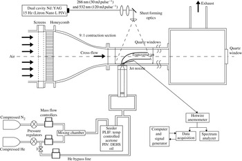
The current experimental set-up utilizes the same low-speed wind tunnel used in previous experiments (Megerian et al.
Reference Megerian, Davitian, de B. Alves and Karagozian2007; Davitian et al.
Reference Davitian, Getsinger, Hendrickson and Karagozian2010a
; Getsinger et al.
Reference Getsinger, Hendrickson and Karagozian2012, Reference Getsinger, Gevorkyan, Smith and Karagozian2014), shown in figure 2. Air from the laboratory was drawn into a centrifugal blower and introduced into a cascade of honeycomb and screens of decreasing mesh size. After flow conditioning, the air entered a 9 : 1 area ratio contraction section that was fitted flush with the test section, resulting in a uniform cross-flow velocity and low turbulence intensity. Hot-wire and stereo particle image velocimetry (PIV) measurements show a resultant maximum test section free-stream velocity
 $U_{\infty }$
of
 $7.0~\text{m s}^{-1}$
and a maximum free-stream turbulence intensity of less than 1.5 %. The dimensions of the test section were 30 cm long and
 $12~\text{cm}\times 12~\text{cm}$
in cross-section. A quartz window was fitted to the top of the test section in order to pass the UV light required for acetone PLIF measurements; details of this measurement technique are discussed in § 2.2. A Plexiglas window was mounted onto one side of the test section for imaging purposes. The entire test section was spray-painted matte black with heat-resistant paint in order to reduce reflection and ablation caused by the laser sheet. Another section of equal dimensions but without optical access was mounted to the end of the primary test section in order to reduce exhaust condition effects on the jet. The second test section was followed by a 30 cm
 $\times$
30 cm
 $\times$
30 cm wooden chamber that was attached to the laboratory’s exhaust system using aluminium ducting. This chamber was fitted with a 90 mm
 $\times$
90 mm quartz window that allowed imaging of the jet cross-section. Care was taken to ensure that pressure differences in the laboratory exhaust system did not affect the test section’s flow (Gevorkyan Reference Gevorkyan2015).
Variable-density transverse jet wind tunnel, with associated data acquisition and optical diagnostic apparatus. One additional tunnel section, of identical dimensions, was situated downstream of the test section shown.

The jet fluid comprised a mixture of nitrogen and helium supplied by two separate gas cylinders, allowing precise control of the jet-to-cross-flow density ratio by varying the gas proportions. The flow from each gas cylinder was controlled using a separate flow controller (Tylan FC-260 and MKS GM50A). The flow controllers fed their respective gases to a passive mixing chamber; the exiting gas mixture was then diverted to an acetone bubbler for PLIF imaging. After exiting the seeder, the gas mixture was exhausted into a Plexiglas pipe below the test section using four symmetrically oriented inlet fittings. Below this pipe was a Plexiglas plenum, housing either a loudspeaker or a piston-based actuator, used in separate studies to apply controlled longitudinal acoustic excitation (M’Closkey et al. Reference M’Closkey, King, Cortelezzi and Karagozian2002; Davitian et al. Reference Davitian, Hendrickson, Getsinger, M’Closkey and Karagozian2010b ; Hendrickson & M’Closkey Reference Hendrickson and M’Closkey2012). Above this Plexiglas plenum was a PVC pipe of sufficient length for full development of laminar pipe flow, alleviating any asymmetries associated with the inlet fittings (Gevorkyan Reference Gevorkyan2015).
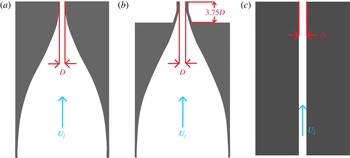
Alternative jet injectors studied: (a) flush nozzle, (b) elevated nozzle and (c) straight pipe.

The well-conditioned gas flow exiting the PVC pipe was fed into the jet injector threaded into the test section. Three separate types of injectors were used in this study, each with an approximately 4 mm exit diameter, as shown in figure 3, including a flush nozzle, an elevated nozzle and a flush straight pipe. Detailed transverse jet structural characteristics associated with all three injectors are described in Getsinger et al. (Reference Getsinger, Gevorkyan, Smith and Karagozian2014). The two nozzles were machined with similar fifth-order polynomial contractions that generate essentially identical thin jet boundary layers at the jet exit in the absence of cross-flow (Megerian et al.
Reference Megerian, Davitian, de B. Alves and Karagozian2007). The only significant difference between the two nozzles was that the exit plane of one was mounted flush with the tunnel floor (figure 3
a), whereas the exit plane of the elevated nozzle protruded into the test section by 3.75 jet diameters (figure 3
b). The protrusion length of the elevated nozzle was such that jet injection occurred outside of the cross-flow boundary layer; for the lowest cross-flow velocity condition explored here,
 $U_{\infty }=1.01~\text{m s}^{-1}$
, the (laminar) wall boundary layer thickness was at its maximum,
 ${\it\delta}_{99\,\%}/D\approx 2.3$
. Further details on the wall boundary layer thicknesses as well as jet flow conditions associated with both flush and elevated nozzles for a range of conditions may be found in Megerian et al. (Reference Megerian, Davitian, de B. Alves and Karagozian2007). The third injector in the present studies consisted of a straight pipe made of aluminium mounted flush with the test section floor. In order to thread this injector into the test section, the PVC pipe mounted between the Plexiglas plenum and the nozzle injectors was necessarily removed due to space constraints, although the pipe alone was verified to have a sufficient length
 $L$
to create a fully developed velocity profile at the jet exit for the Reynolds numbers studied in this experiment (
 $L/D=155$
). The Reynolds number of the jet was based on the bulk jet velocity,
 $U_{j}$
, determined from the specified mass flow rate of the gas mixture, the mixture viscosity and the density
 ${\it\rho}_{j}$
of the jet. During acetone PLIF experiments, the effect of acetone on jet density and transport properties was taken into account; details may be found in Getsinger (Reference Getsinger2012). The jet Reynolds number was kept constant at
 $Re_{j}=1900$
for the cases presently studied, while the jet-to-cross-flow density ratio
 $S$
was varied, based on the proportions of acetone, helium and nitrogen in the jet, to determine the effect of this parameter on mixing efficiency (
 $0.35\leqslant S\leqslant 1$
), since it clearly affects transverse jet shear layer stability (Getsinger et al.
Reference Getsinger, Hendrickson and Karagozian2012) and structure (Getsinger et al.
Reference Getsinger, Gevorkyan, Smith and Karagozian2014). Jet-to-cross-flow momentum flux ratio
 $J$
was varied independently of density ratio by altering the cross-flow speed at fixed jet conditions (fixed
 $S$
and
 $Re_{j}$
). For a given density ratio, jet fluid mass flow rates were identical among different momentum flux ratios, and were very similar for different injectors. It should be noted, however, that slight differences in jet exit diameter resulted in small mean jet velocity differences among the injectors for fixed jet Reynolds number (7 % maximum diameter difference due to machining error among all injectors). Yet, given the transverse jet’s strong dependence on momentum flux ratio
 $J$
(Kamotani & Greber Reference Kamotani and Greber1972; Smith & Mungal Reference Smith and Mungal1998; Megerian et al.
Reference Megerian, Davitian, de B. Alves and Karagozian2007) and far lesser dependence on jet Reynolds number (Megerian et al.
Reference Megerian, Davitian, de B. Alves and Karagozian2007; Getsinger et al.
Reference Getsinger, Gevorkyan, Smith and Karagozian2014), small differences in mean jet exit velocity with fixed
 $J$
,
 $Re_{j}$
and
 $S$
did not significantly affect behaviour for the different injectors.
2.2. Planar optical diagnostics
Jet fluid concentration measurements obtained using PLIF of acetone vapour seeded into the jet was the primary method for evaluating various mixing metrics for transverse jets of varying density and momentum flux ratios. The general set-up for optical measurements is included in figure 2, and additional details may be found in Getsinger (Reference Getsinger2012), Getsinger et al. (Reference Getsinger, Gevorkyan, Smith and Karagozian2014) and Gevorkyan (Reference Gevorkyan2015). The light source for PLIF was a dual-cavity Q-switched Nd : YAG laser (Litron Nano L PIV) equipped with second- and fourth-harmonic generators for simultaneous output at 266 and 532 nm. Each cavity of the laser had an output of approximately
 $30~\text{mJ}~\text{pulse}^{-1}$
at 266 nm (UV) and
 $120~\text{mJ}~\text{pulse}^{-1}$
at 532 nm in an 8 ns full width at half-maximum (FWHM) period. While the maximum repetition rate for the laser was 15 Hz, the maximum recording rate among all the different measurements was 7.5 Hz in order to decrease ablation of the paint applied to the test section floor as well as to ensure statistical independence of the images.
The beam from the laser was formed into a thin divergent sheet using two spherical lenses, a turning mirror and an
 $f=-10$
mm cylindrical lens before entering the test section via the upper quartz window. The cylindrical lens could be rotated by 90°, allowing measurements of both the jet centreplane (
 $y=0$
) and the jet cross-sectional
 $y$
–
 $z$
plane at any desired constant
 $x/D$
position within the test section. Traversal of the sheet in the cross-flow (
 $x$
) direction was accomplished using a lead-screw/stepper motor device mounted to the bottom of the wind tunnel, allowing movement of the entire test section while keeping the optical set-up stationary.
Acetone has been utilized as a molecular tracer for temperature, pressure and concentration measurements in gaseous flows for over two decades (Lozano Reference Lozano1992; Smith & Mungal Reference Smith and Mungal1998; Thurber et al.
Reference Thurber, Grisch, Kirby, Votsmeier and Hanson1998; Su & Mungal Reference Su and Mungal2004). For isothermal, low-Mach-number flows in atmospheric conditions in which the excited fluid medium is optically thin, fluorescence intensity is linearly proportional to both the laser fluence and acetone concentration, assuming laser light absorption saturation is not reached (Lozano Reference Lozano1992; Lozano, Yip & Hanson Reference Lozano, Yip and Hanson1992). For the present acetone PLIF measurements, the laser beam was directed at two dichroic mirrors mounted prior to the sheet-forming optics. This dichroic mirror set reflected the 266 nm UV light while removing the majority of the 532 nm green light used for PIV measurements. The UV light that reflected off the dichroic mirrors was then passed through a 3 mm thick UV-grade fused silica window, which was oriented such that a small (
 ${\approx}7\,\%$
) portion of the UV beam was reflected to a pyroelectric joulemeter for real-time energy measurement recorded to a computer. The measured
 $1/\text{e}^{2}$
thickness of the laser sheet (measured using the knife-edge traversal technique) was approximately
 $400{-}900~{\rm\mu}\text{m}$
in the camera’s field of view. In order to ensure that the mixing metrics’ trends were not significantly affected by the spatial resolution of the data, several key datasets of much higher in-plane and out-of-plane resolution were taken, with a
 $360{-}450~{\rm\mu}\text{m}$
sheet thickness, producing
 $34~{\rm\mu}\text{m}~\text{pixel}^{-1}$
resolution. The results for various mixing metrics were compared to the lower-resolution data for both equidensity (
 $S=1.0$
) and low-density (
 $S=0.35$
) JICF conditions. The trends among the higher-resolution and lower-resolution datasets were found to be the same for all flow conditions, with less than a 1 % quantitative difference in equidensity mixing metrics. As expected, resolution requirements for
 $S=0.35$
were higher, and approximately a 10 % difference in the values of mixing metrics between high- and low-resolution cases was observed. Nevertheless, none of the conclusions or trends observed in the lower-resolution data were found to be affected by improving resolution. A more in-depth discussion on the resolution of this experimental set-up and the relevant flow scales in this study may be found in Gevorkyan (Reference Gevorkyan2015).
PLIF images were captured using a 14-bit charge-coupled device (CCD) camera (LaVision Imager proX) with
 $1600\times 1200$
pixel resolution, equipped with an external image intensifier (LaVision IRO) to increase the signal-to-noise ratio (SNR). The cross-sectional images were taken with a Nikon 200 mm lens at
 $f/4.0$
. The centreplane images were taken with a Nikon 50 mm lens at
 $f/2.0$
equipped with a Vivitar
 $+2$
dioptre close-up lens. All lens configurations utilized a bandpass filter to isolate the fluorescence signal.
Centreplane images were taken with the camera located on one side of the test section. The resolution of the centreplane images ranged from 140 to
 $170~{\rm\mu}\text{m}~\text{pixel}^{-1}$
after
 $2\times 2$
hardware binning was administered to increase the SNR. This resolution variation was necessary to capture enough downstream data for the higher-penetrating pipe flow configuration, and is not expected to significantly affect the statistical quantities for reasons mentioned previously. The cross-sectional (
 $y$
–
 $z$
plane) images were taken by orienting the camera at the end of the wind tunnel looking upstream, in the negative
 $x$
direction. Cross-sectional data resolution ranged from 120 to
 $160~{\rm\mu}\text{m}~\text{pixel}^{-1}$
after
 $2\times 2$
hardware binning. The image intensifier was gated for 200 ns, chosen to be short enough to negate the signal contribution of phosphorescence, which accumulates over much larger time scales than the fluorescence. Phosphorescence is also strongly quenched by oxygen, which was present in any mixed-fluid regions of the jet. A temporal spacing of 50 ns was set between the two laser pulses, and both laser pulses were included in the 200 ns gate window, resulting in a doubled fluorescence signal with negligible motion blurring (less than
 $2~{\rm\mu}\text{m}$
maximum flow movement within this time span).
Acetone seeding was accomplished by bubbling the mixture of helium and nitrogen from the mixing chamber through two separate seeders connected in series, used to ensure saturation of acetone vapour. The details of the method used for determination of the acetone mole fraction and its effects on the gas mixture may be found in Getsinger (Reference Getsinger2012), Getsinger et al. (Reference Getsinger, Gevorkyan, Smith and Karagozian2014) and Gevorkyan (Reference Gevorkyan2015). The raw PLIF data were corrected for camera dark noise, ambient background light and laser sheet reflections, non-uniformity of the mean laser sheet energy profile, UV light attenuation due to absorption, global pulse-to-pulse laser sheet energy fluctuations, and the flat-field response of the imaging system. UV light absorption correction was particularly important to quantify for highly penetrating jets in cross-flow at high momentum flux ratios. The effective absorption length, per Beer’s law, was determined using an iterative method. The absorption length associated with the most severe degree of absorption by a highly penetrating jet, for the equidensity
 $J=41$
flush nozzle-injected JICF, was used to correct PLIF concentration data for a range of operating conditions, and was found to produce a more uniform potential core concentration. The corrected centreplane images were then normalized to the fluorescence signal in the jet potential core, resulting in jet fluid concentration
 $C$
being scaled with a range from pure jet fluid (
 $C/C_{o}=1$
) to pure cross-flow fluid (
 $C/C_{o}=0$
), where
 $C_{o}$
is the concentration of pure jet fluid at the jet exit and within the potential core. The cross-sectional images resulting from the correction scheme were converted to jet fluid concentration by comparing common lines of data between the centreplane and cross-sectional images. Details of the correction method can be found in Getsinger (Reference Getsinger2012) and Gevorkyan (Reference Gevorkyan2015). All acetone PLIF data were filtered with a
 $5\times 5$
median filter administered after processing. This filter was found to be the more effective at preserving gradients while decreasing noise when compared to traditional linear filters, which is consistent with the findings of Ghandhi (Reference Ghandhi2006).
3. Mixing metrics
The aforementioned acetone PLIF imaging results in the ability to explore transverse jet structural characteristics for a range of operating conditions, including momentum flux ratio
 $J$
, density ratio
 $S$
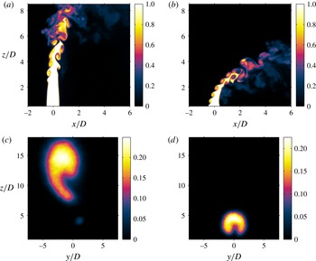
and injector type. Details on these structural characteristics, seen via centreplane-based and cross-sectional PLIF imaging, are described in Getsinger (Reference Getsinger2012), Getsinger et al. (Reference Getsinger, Gevorkyan, Smith and Karagozian2014) and Gevorkyan (Reference Gevorkyan2015). As noted above, there is a strong correlation between the transverse jet’s upstream shear layer instabilities and vorticity rollup and the cross-sectional formation and evolution of the CVP. Sample results for this correspondence are shown in figure 4, for a flush nozzle-generated, equidensity transverse jet with upstream shear layers known to be convectively unstable (
 $J=41$
, figure 4
a,c) and absolutely unstable (
 $J=5$
, figure 4
b,d). These and other JICF flow conditions (
 $2\leqslant J\leqslant 41$
,
 $0.35\leqslant S\leqslant 1.0$
and
 $1000\leqslant Re_{j}\leqslant 6500$
), for all three injectors, show remarkable correspondence for jets having weak, convectively unstable shear layers and delayed upstream shear layer vorticity rollup with an asymmetric or non-existent CVP in the mean jet cross-section. An example of this kind of cross-section is shown in figure 4(c). Similarly, there is correspondence for jets with absolutely unstable shear layers and rapid or immediate shear layer vorticity rollup with formation of a clear, symmetric CVP in the cross-section; an example of this is shown in figure 4(d). Many additional examples of these correspondences are shown in Getsinger et al. (Reference Getsinger, Gevorkyan, Smith and Karagozian2014).
Instantaneous centreplane (side view) acetone PLIF imaging of the flush nozzle-generated JICF with
 $Re_{j}=1900$
and density ratio
 $S=1.0$
for (a)
 $J=41$
and (b)
 $J=5$
. Cross-sectional jet slices at
 $x/D=5.5$
, averaged over 300 images, for the same flush nozzle and flow conditions, are shown for (c)
 $J=41$
and (d)
 $J=5$
.

PLIF imaging may be used in the present studies for detailed quantification of mixing characteristics under different JICF operating conditions. It is noted that, at the relatively low Reynolds numbers explored, transport processes are predominantly diffusion-limited, hence flow alterations having the potential to alter concentration gradients can affect mixing processes. Determining the mixing metric(s) best suited for transitional or turbulent flow fields has been a topic of discussion in the fluid dynamics community for decades. As mentioned previously, several of the mixing metrics traditionally applied to transverse jets rely on mean quantities on the centreplane (
 $y=0$
) of the jet. Centreplane mixing metrics are an extension of the typical free jet analysis in which the centreline concentration decay is a good indicator of the overall evolution of the jet due to entrainment and engagement of the jet with the surrounding fluid. Since the transverse jet has a trajectory that varies significantly depending on flow-field properties such as
 $J$
and
 $S$
, however, a consistent definition of the centreline of the jet must be formulated to determine mixing efficiency using centreplane metrics. In this experiment, similar to the work of Smith & Mungal (Reference Smith and Mungal1998), the transverse jet trajectory is determined from centreplane scalar concentration data using a least-squares power-law fit to the loci of maximum jet fluid concentration values found in the jet trajectory-normal (
 $n$
) direction. This was accomplished by first fitting a power law to the maximum values in each vertical column (constant
 $x$
) of data from the image array, using the relation
 $z/D=A(x/D)^{m}$
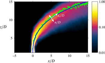
(Margason Reference Margason1993). We then iterated on the fit by finding the maximum trajectory-normal concentration value at each position on the trajectory, where the fit typically converged after three iterations. Figure 5 is a typical result of this fitting, with a mean centreplane concentration image, loci of the maximum concentration values and power-law fit shown for the
 $J=20$
equidensity JICF. Corresponding jet trajectory (
 $s_{c}$
) and jet-normal (
 $n$
) parameters are shown in this figure. It should be noted that this method of trajectory fitting does not work as well for the lowest momentum flux ratio studied here,
 $J=2$
, for which there was significant interaction of the jet with the wall boundary layer.
Mean scalar concentration image in the
 $y=0$
centreplane, with colour-bar values corresponding to local concentration
 $C/C_{o}$
, for the
 $J=20$
,
 $S=1.00$
transverse jet. Averaging takes place over 300 images. Light green data points on this mean jet image show the loci of scalar maxima, while the blue line shows the power-law curve fit, with corresponding normal (
 $n$
) and trajectory (
 $s_{c}$
) coordinates scaled by diameter
 $D$
.

After the trajectory of the jet is determined, a number of centreplane mixing metrics may be quantified along the trajectory. The actual distance along the jet trajectory coordinate
 $s_{c}$
can be determined using numerical integration of the power-law fit. Among the most commonly used centreplane mixing metrics is the decay of the maximum mean concentration along the jet trajectory (Smith & Mungal Reference Smith and Mungal1998; Su & Mungal Reference Su and Mungal2004), and this may be determined from scalar concentration measurements. Theoretically, the rate of spatial decay of this concentration value is related to the rate of entrainment of cross-flow into the jet, as noted by Shan & Dimotakis (Reference Shan and Dimotakis2006). Yet these researchers also note that mixing in a transitional and/or turbulent flow field is an inherently unsteady process, and that averaging over time could potentially obscure instantaneous scalar structure information, yielding erroneous conclusions about mixing efficiency. This issue will be explored in detail in the present studies.
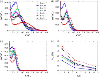
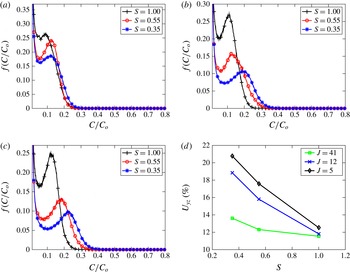
Instantaneous mixing metrics for the JICF are most logically applied to the cross-section of the jet, especially further downstream, where the jet tends to be oriented more closely with the cross-flow direction and thus where the vertical laser sheet is more closely perpendicular to the jet trajectory. Yet application of instantaneous metrics to the centreplane data could also reveal information about the effect of the off-centreplane jet fluid distribution on more common mixing quantification such as mean centreline concentration decay. One of the most widely used mixing metrics for scalar data is the spatial p.d.f., defined as a histogram of the instantaneous scalar data normalized such that the area under the histogram curve is equal to unity. Each instantaneous p.d.f. is then averaged over the entire dataset to obtain the average spatial p.d.f. For a perfectly mixed fluid mixture, the spatial p.d.f. would theoretically reveal a Dirac delta function at the spatial mean value of the scalar. For completely unmixed fluids, two separate Dirac delta functions would be found at scalar values of zero and one. Therefore, increased levels of mixing in a closed system result in the appearance of a preferred (most probable) value of the scalar, and an evolution towards and eventual localization of that preferred value at the mean. Smith & Mungal (Reference Smith and Mungal1998) applied this metric to JICF centreplane data in order characterize and compare the spatial evolution of the mixing characteristics of the transverse jet, while Shan & Dimotakis (Reference Shan and Dimotakis2006) utilized spatial p.d.f.s of cross-sectional scalar data to determine mixing efficiency variation with increasing Reynolds number for
 $R=10$
transverse jets.
Since the transverse jet is an open boundary system, special attention needs to be given to the method of application of mixing metrics such as the p.d.f. that are better suited for closed boundary systems. The global mass or concentration ratio between the two fluids mixed in a closed boundary system does not change, resulting in a constant global mean value of the scalar being measured. But this is not necessarily true for an open boundary system such as the jet in cross-flow. As demonstrated in the work of Shan & Dimotakis (Reference Shan and Dimotakis2006), mass conservation applied to a control volume containing the entire equidensity jet in cross-flow results in determination of a mean scaled jet fluid concentration value,
 ${\hat{C}}/C_{o}$
, which is a function of the jet-to-cross-flow velocity ratio
 $R$
, the cross-sectional area
 $A_{j}$
of the jet exit and the cross-sectional area
 $A_{cs}$
of the control surface enclosing the mixed jet cross-section at a downstream location
 $x$
, oriented in the
 $y{-}z$
plane:
 $$\begin{eqnarray}\frac{{\hat{C}}(x)}{C_{o}}\simeq R\frac{A_{j}}{A_{cs}(x)}.\end{eqnarray}$$
This relation assumes that the average component of jet velocity perpendicular to the control surface is approximately equal to the cross-flow speed
 $U_{\infty }$
. This is a reasonably accurate assumption for
 $x\gg D$
, far downstream of jet fluid injection, especially for relatively small values of
 $R$
, and it can serve as a general (though imperfect) guide for trends in mean concentration along the jet trajectory. Yet in order to compare the mixing statistics of jet slices at different spatial locations
 $x$
or
 $s_{c}$
, and for the range of
 $J$
and
 $S$
values explored, the mean value of the scalar evaluated over the selected interrogation area,
 $\overline{C}$
, should be the same for all flow conditions. To accomplish such direct comparisons of mixing metrics in the present experiments, the size of the cross-sectional interrogation area
 $A_{i}$
was varied such that the mean value of the scalar over this area,
 $\overline{C}$
, was matched among different cases and at different instants of time. An elaboration on this procedure for matching mean concentrations for cross-sectional images is provided in § 4.3.
Although the p.d.f. is an important tool for visualizing the level of mixing as well as the distribution of jet fluid, a global quantitative value of the degree of mixing proves valuable as well. Several of these types of global mixing metrics exist, but one of the most widely used is the unmixedness
 $U$
evaluated from a slice of the flow field taken at a location
 $x$
, for example, in the
 $y{-}z$
plane (Danckwerts Reference Danckwerts1952):
 $$\begin{eqnarray}U_{yz}(x)=\frac{1}{L_{y}L_{z}}\iint \frac{(C/C_{o}-\overline{C}/C_{o})^{2}}{(\overline{C}/C_{o})(1-\overline{C}/C_{o})}\,\text{d}y\,\text{d}z.\end{eqnarray}$$
Here
 $C/C_{o}$
is the local scaled measure of instantaneous jet fluid concentration at a pixel element situated at location
 $(y,z)$
and, as before,
 $\overline{C}/C_{o}$
is the spatial average of that concentration taken over the interrogation area
 $A_{i}$
in the
 $y{-}z$
plane. The product
 $L_{y}L_{z}$
is a representation of the physical size of the interrogation area
 $A_{i}$
over which the calculation is administered. The unmixedness is essentially a spatial variance measurement normalized by the variance obtained when the flow field is stirring but not mixing or diffusing (Dimotakis & Miller Reference Dimotakis and Miller1990), and thus is an attempt to quantify the information contained in the p.d.f. in a compact form. Just as for the p.d.f., spatial mean matching was also administered for unmixedness in order to more accurately compare mixing processes among transverse jets with different jet-to-cross-flow mass/molar flux ratios, per the discussion above. Such matching involves adjusting
 $L_{y}$
and
 $L_{z}$
for different flow conditions by adding or subtracting zero-valued pixels to create the same mean (
 $\overline{C}$
) at all cross-section locations
 $x$
. Similar to the p.d.f., unmixedness calculations were applied to each instantaneous image and averaged over each dataset.
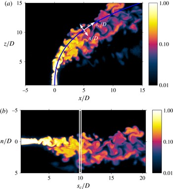
(a) Instantaneous scalar centreline trajectory in the
 $y=0$
centreplane of the transverse jet for
 $J=20$
and
 $S=1.00$
. As in figure 5, the blue line shows the power-law curve fit for the corresponding mean jet image. (b) Instantaneous image transformed into the
 $s_{c}/D$
–
 $n/D$
coordinate system with an example of a thin interrogation area slice centred at
 $s_{c}/D=10$
, of total width 0.25, used to evaluate centreplane unmixedness
 $U_{c,sn}$
.

Since centreplane PLIF images do not capture the extent of the jet’s cross-section and therefore do not contain all of the jet fluid introduced into the cross-flow, this approach to mean matching has less of a physical basis for centreplane scalar measurements. Nevertheless, it is useful to determine if trends in cross-sectional mixing metrics such as unmixedness correspond to centreplane-based mixing quantification. Hence, centreplane jet fluid concentration values
 $C/C_{o}$
were evaluated over narrow slices of the jet in the transformed jet-normal direction
 $n$
at various distances along the jet trajectory direction
 $s_{c}$
, as shown for an example of an instantaneous centreplane image in figure 6(a,b). With a fixed width of the narrow interrogation area (seven pixel widths, corresponding to
 $s_{c}/D\simeq 0.25$
), one can alter the height of the region capturing jet fluid in the normal direction
 $n$
so as to have equivalent means
 $\overline{C}$
among different jet locations and flow conditions. A transformation into the
 $n/D$
–
 $s_{c}/D$
coordinate system, as shown in figure 6(b), simplifies this evaluation. In this way, an equivalent centreplane unmixedness
 $U_{c}$
may be evaluated using a relation similar to (3.2) but in the
 $x{-}z$
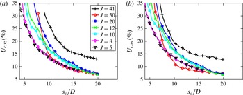
plane. In the present studies, a seven-pixel-wide interrogation area was determined to be sufficiently thin to replicate capture of the jet by the cross-sectional laser sheet imaging, but at the same time being sufficiently thick to enable statistical convergence (Gevorkyan Reference Gevorkyan2015). Further details on this mean matching approach for centreplane images such as those in figure 6 are provided in § 4.4.
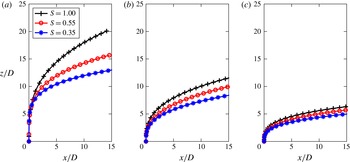
Scalar centreline trajectories of flush nozzle-injected transverse jets of various density ratios, for (a)
 $J=41$
, (b)
 $J=12$
and (c)
 $J=5$
.

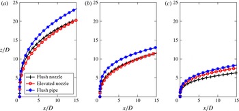
Scalar centreline trajectories of
 $S=1.00$
transverse jets injected from flush nozzle, elevated nozzle and flush straight pipe injector configurations, for (a)
 $J=41$
, (b)
 $J=12$
and (c)
 $J=5$
.

It should be noted that other mixing metrics have been utilized by various groups to determine mixing efficiency in open boundary systems. The spatial mixing deficiency (SMD) (Boss Reference Boss1986), for example, is essentially a normalized standard deviation measurement; a perfectly mixed fluid should have no fluctuation about the mean value, resulting in a zero standard deviation or SMD. Yet the SMD as typically defined is not ideal for quantification of mixing for scalar data of open boundary systems, since its normalization to the mean value
 $\overline{C}/C_{o}$
does not take into account the scalar values for unmixed fluids, potentially yielding erroneous conclusions about the relative level of mixing. On the other hand, if the mean value
 $\overline{C}/C_{o}$
is matched among different JICF cases, SMD and
 $U$
should (and do) exhibit the same trends in mixing. For this reason,
 $U$
and p.d.f. rather than SMD were used as the primary instantaneous mixing metrics in this study.
4. Results
4.1. Scalar centreline trajectories
Scalar centreline trajectories are important to quantify for the range of flow and injection systems explored here, given that, for a transverse jet,
 $s_{c}$
effectively represents the distance along which jet fluid is exposed to the cross-flow and thus liable to mix. Moreover, early JICF studies (Holdeman Reference Holdeman1993; Margason Reference Margason1993) suggest a correspondence between jet penetration (or a higher trajectory) and improved mixing. And while many transverse jet experiments over the years have studied the effects of momentum flux ratio
 $J$
and jet Reynolds number on jet trajectory, as summarized in Karagozian (Reference Karagozian2010), few have separately examined the effects of density ratio or injector geometry on trajectory in a systematic way.
The scalar centreline trajectories for
 $Re_{j}=1900$
transverse jets injected from the flush nozzle, for several different density and momentum flux ratios, are plotted in figure 7. Note that here and in other trajectory plots, centreline concentration decay plots and centreplane-based mixing metrics, data point markers do not represent actual resolution of data, which is much finer than shown. It has been previously demonstrated for the flush nozzle (Getsinger et al.
Reference Getsinger, Hendrickson and Karagozian2012, Reference Getsinger, Gevorkyan, Smith and Karagozian2014) that absolutely unstable jet shear layer conditions correspond to a density ratio of
 $S=0.35$
for all momentum flux ratios
 $J$
, as well as for all values of
 $S$
when
 $J\leqslant 10$
. Otherwise, for
 $J>10$
and
 $S\geqslant 0.55$
, the conditions correspond to convectively unstable upstream shear layers. The data in figure 7 show that, at a fixed
 $J$
, reducing
 $S$
(and thus increasing the velocity ratio
 $R$
for a fixed jet Reynolds number) had the effect of reducing penetration, or lowering the trajectory of the jet. This reduction was particularly significant at higher fixed
 $J$
values. The reduction in jet penetration with a decrease in density ratio was consistent with the fact that, in keeping the momentum flux ratio constant at a fixed
 $Re_{j}$
, decreasing the density ratio required both jet and cross-flow velocities to be increased, in some cases, significantly. These changes simultaneously reduced the cross-flow boundary layer thickness, thus enabling a more immediate influence of the cross-flow in turning the jet, hence reducing penetration. Cross-flow entrainment variation could also affect jet trajectory, but entrainment differences would have to be quantified to verify this contention. The effect of an increased jet velocity at lower jet densities could also affect the potential core, and hence mixing; these issues will be analysed in § 4.2.
Figure 8 highlights the effect of injector configuration on the trajectory of equidensity transverse jets for several different momentum flux ratios. Per Getsinger et al. (Reference Getsinger, Gevorkyan, Smith and Karagozian2014), only the
 $J=5$
condition shown for the flush nozzle and flush pipe represented a JICF with an absolutely unstable upstream shear layer; the effect of the external co-flow significantly weakens the elevated jet’s shear layer instabilities at
 $J=5$
. The flush pipe-injected jets were observed overall to penetrate farther into the cross-flow than either the flush nozzle- or elevated nozzle-injected jets for the higher range of momentum flux ratios shown (
 $J=41$
and 12), consistent with a DNS study by Muppidi & Mahesh (Reference Muppidi and Mahesh2005) on the effects of jet velocity profile on the trajectories of the equidensity JICF. This observation suggested that jets with a parabolic velocity profile and thicker jet boundary layer at its exit could penetrate more deeply than for other jets at the same
 $J$
and
 $Re_{j}$
values, possibly in part due to the higher centreline velocity for the parabolic profile if
 $U_{j}$
is matched. Interestingly, the only condition in the experiments for which the flush pipe approached the trajectories of the nozzle-generated jets was for the absolutely unstable conditions (for the flush jets) at
 $J=5$
, where experiments have shown that the upstream jet momentum thickness for the flush nozzle is relatively large (Megerian et al.
Reference Megerian, Davitian, de B. Alves and Karagozian2007) and where recent simulations (Mahesh & Iyer Reference Mahesh and Iyer2013) suggest that cross-flow fluid may travel into the flush jet orifice itself at such strong cross-flow conditions. It should be noted that the momentum flux was matched here using mass-averaged (and not momentum-averaged) velocity, and this also could have contributed to differences observed here. Figure 8(a,b) also indicates that, for equidensity higher momentum flux ratios (
 $J=41$
and 12), the trajectory of the flush nozzle was similar to that of the elevated nozzle, suggesting a minimal influence of the cross-flow boundary layer on trajectory for flush injection in this regime. At the lower value of
 $J=5$
, the increased cross-flow velocity has been documented (Megerian et al.
Reference Megerian, Davitian, de B. Alves and Karagozian2007) to create a greater degree of vertical co-flow upstream of the elevated nozzle, and this probably caused the slight difference between the flush and elevated nozzle trajectories. The implications of these observations for jet mixing and entrainment will be explored in § 4.2.
While the jet trajectories shown in figures 7 and 8 employed non-dimensionalization by diameter
 $D$
, alternative length scales can account for flow conditions, especially given that the high-
 $J$
transverse jet interacts with the cross-flow over a longer spatial distance (
 $s$
or
 $s_{c}$
) than does a low-
 $J$
transverse jet, certainly affecting jet–cross-flow interactions and the evolution of vortical structures (Getsinger et al.
Reference Getsinger, Gevorkyan, Smith and Karagozian2014). Early experimental studies on the JICF (Keffer & Baines Reference Keffer and Baines1963) suggest that using the product of momentum flux ratio and jet diameter,
 $JD$
, to scale jet trajectory leads to successful data collapse in the range
 $36\leqslant J\leqslant 100$
, although later experiments and simulations (Broadwell & Breidenthal Reference Broadwell and Breidenthal1984; Smith & Mungal Reference Smith and Mungal1998; Hasselbrink Reference Hasselbrink1999; Muppidi & Mahesh Reference Muppidi and Mahesh2005) indicate improved data collapse with
 $RD$
or
 $\sqrt{J}D$
scaling. Yet
 $RD$
scaling appears to be relevant only for relatively high
 $R$
values; per Smith & Mungal (Reference Smith and Mungal1998), scaled trajectories for
 $R=5$
tend to differ from those for
 $R\geqslant 10$
. The computational studies of Muppidi & Mahesh (Reference Muppidi and Mahesh2005) show that transverse jets of equivalent
 $R$
but different cross-flow and jet velocity profiles have different trajectories; as noted earlier, jets with thinner boundary layers tend to penetrate less, and conditions where the cross-flow boundary layer thickness is smaller, due to increased cross-flow velocity, also have lower penetration. Interestingly, even when an additional length scale is introduced to represent these profile differences, the
 $RD$
-based trajectory collapse occurs for a higher velocity ratio,
 $R=5.7$
, but is much less successful for
 $R=1.52$
. Recent JICF scaling analysis by Forliti, Salazar & Bishop (Reference Forliti, Salazar and Bishop2015) suggests use of a scale factor
 $B$
which is a function of
 $J$
as well as empirical drag and entrainment coefficients, but this too focuses on somewhat higher values of
 $R$
(
 ${\geqslant}4$
).
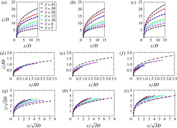
Figure 9 shows the trajectories of equidensity transverse jets injected from all three injectors in the present studies for
 $41\geqslant J\geqslant 5$
, using different scaling of the physical coordinates via
 $D$
,
 $JD$
and
 $\sqrt{J}D$
. If any of these parameters were to capture the relevant physics associated with the jet trajectory (e.g. entrainment or spreading rate), trajectory data would collapse onto a single curve and the flow would be considered to be self-similar. It is clear from figure 9 that none of the length scales used to scale physical coordinates achieved significant data collapse in this rather broad range of
 $J$
values:
 $JD$
scaling seemed to produce the highest degree of data collapse, especially for the flush and elevated nozzle-injected cases in the range
 $41\leqslant J\leqslant 8$
;
 $J=5$
data also appeared to collapse reasonably well for the flush nozzle with
 $JD$
scaling, but the
 $J=5$
elevated nozzle-injected jet penetrated more deeply into the cross-flow in
 $JD$
-scaled space as compared with the other cases. The elevated JICF at this low-
 $J$
condition corresponds to very weak shear layer instabilities, in contrast to absolute instabilities for the flush injectors. The degree of data collapse with
 $JD$
scaling for the flush pipe-based trajectories was not as favourable in this flow regime as it was for other injectors, consistent with trajectory trends shown in figure 8.
Scalar centreline trajectories of
 $S=1.00$
transverse jets for various momentum flux ratios, for various injectors: (a,d,g) flush nozzle, (b,e,h) elevated nozzle and (c,f,i) flush straight pipe. Data are shown for various physical coordinate scalings:
 $D$
,
 $JD$
and
 $\sqrt{J}D$
, in (a–c), (d–f) and (g–i), respectively.

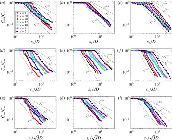
Maximum mean concentration (
 $C_{m}/C_{o}$
) decay trends along the scalar centreline trajectory coordinate
 $s_{c}$
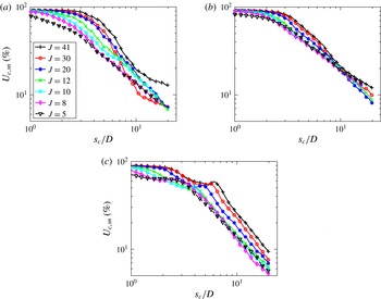
for equidensity transverse jets at various momentum flux ratios, for various injectors: (a,d,g) flush nozzle, (b,e,h) elevated nozzle and (c,f,i) flush straight pipe. Data are shown for various physical coordinate scalings:
 $D$
,
 $JD$
and
 $\sqrt{J}D$
in (a–c), (d–f) and (g–i), respectively.

4.2. Maximum mean concentration decay
The decay in the maximum mean scalar concentration
 $C_{m}$
along the jet centreline has been commonly used to characterize mixing for transverse jets (Smith & Mungal Reference Smith and Mungal1998); the centreplane-based acetone PLIF images in the present study may be used to extract such data. Figure 10 highlights the maximum mean concentration decay trends in
 $C_{m}/C_{o}$
along the scaled centreplane trajectory
 $s_{c}/D$
for equidensity transverse jets injected from all three injectors. In figure 10, the trajectory coordinate
 $s_{c}$
is used rather than the downstream distance
 $x$
, given the ability for the former to represent local exposure of jet fluid to cross-flow, and hence to represent the evolution of molecular mixing more effectively. More direct comparisons of maximum centreline concentration decay,
 $C_{m}/C_{o}$
, are also more straightforward among different flow conditions with
 $s_{c}$
-based quantification. Mixing metric evolution with downstream distance
 $x$
will be examined in a later section. Figure 10 displays scaling of distance
 $s_{c}$
by
 $D$
,
 $JD$
and
 $\sqrt{J}D$
. Simple plotting of centreline concentration decay as a function of
 $s_{c}/D$
, in figure 10(a–c), demonstrated the effects of injector and
 $J$
values on the length of the potential core, defined as the locus at which the concentration
 $C/C_{o}$
started to drop below unity. On the other hand, scaling of downstream decay with
 $s_{c}/\sqrt{J}D$
, shown in figure 10(g–i), enabled effective matching of potential cores for flush nozzle and flush pipe injectors for virtually all flow conditions, and thus a more straightforward comparison of concentration decay slopes downstream of the potential core. This centreline concentration decay scaling with
 $\sqrt{J}D$
is also observed for the flush nozzle-injected JICF at higher momentum flux ratios,
 $25\leqslant J\leqslant 100$
(Smith & Mungal Reference Smith and Mungal1998), to enable potential core lengths to be matched. The present studies showed that none of the scaling shown in figure 10 enabled collapse of potential core lengths for the elevated nozzle, however, consistent with the influence of vertical co-flow at higher cross-flow velocities. Scaling of centreline concentration decay with
 $JD$
(figure 10
d–f) did not allow collapse of the potential cores for any injector.
Reference lines shown in figure 10 represent concentration decay as various power laws:
 $s_{c}^{-1.3}$
, observed by Smith & Mungal (Reference Smith and Mungal1998) for transverse jets at high
 $J$
in the near field, prior to the aforementioned ‘branch’ point;
 $s_{c}^{-2/3}$
, observed by these researchers for decay after the branch point; and
 $s_{c}^{-1}$
, representing concentration decay for the free jet as well as the straight pipe-generated JICF at high
 $J$
(Su & Mungal Reference Su and Mungal2004). The present results suggested differing decay scaling for the various injectors and flow conditions. For the flush nozzle at
 $J=41$
and especially at
 $J=30$
, there was a greater near-field rate of concentration decay than even
 $s_{c}^{-1.3}$
scaling, after which there appeared to be a branch point, and then concentration decay at a lower rate, closer to
 $s_{c}^{-2/3}$
scaling. It is noted that both
 $J=41$
and
 $J=30$
convectively unstable transverse jets created by the flush nozzle had clearly asymmetric cross-sections (Getsinger et al.
Reference Getsinger, Gevorkyan, Smith and Karagozian2014; Gevorkyan Reference Gevorkyan2015). Smith & Mungal (Reference Smith and Mungal1998) observe similar branch points for
 $J>25$
, attributing them to the transverse jet’s shifting from jet-like behaviour in the near field to wake-like behaviour in the far field (Hasselbrink & Mungal Reference Hasselbrink and Mungal2001). Smith & Mungal (Reference Smith and Mungal1998) find the ‘branch point’ to occur at
 $s_{c}/JD=0.3$
, very close to the branch point observed in the present studies for
 $J=41$
and
 $J=30$
(
 $s_{c}/JD\approx 0.33$
) as shown in the
 $JD$
-scaled flush nozzle-injected concentration decay trends in figure 10. There were no other injectors or equidensity jet conditions for which a branch point was observed here; studies by Su & Mungal (Reference Su and Mungal2004) for flush pipe- and elevated pipe-injected transverse jets similarly show a lack of branch point behaviour at high momentum flux ratios.
There was hence a ‘crossing over’ of decay lines for varying
 $J$
in the flush nozzle-injected transverse jet
 $C_{m}/C_{o}$
decay trends in the present experiments, more apparent in the plot of
 $C_{m}/C_{o}$
as a function of
 $s_{c}/D$
in figure 10(a). This ‘crossing over’ is also observed by Smith & Mungal (Reference Smith and Mungal1998) at higher
 $J$
values, and is postulated to be the physical mechanism behind a minimum in flame length observed to occur at a specific value of
 $R$
in reactive JICF experiments (with minima produced for flows in the range
 $10<R<20$
, depending on the chemical reaction). One could argue from the present results that, for a (relatively low) critical value of
 $C_{m}/C_{o}$
associated with a well-mixed jet,
 $J=30$
might provide a minimum in flame length as compared with other flow conditions, although to our knowledge there are no reactive experiments showing critical minimum flame lengths in this regime for
 $J$
.
At lower
 $J$
values for the flush nozzle, the JICF concentration decay rate scaled between
 $s_{c}^{-1.3}$
and
 $s_{c}^{-1}$
, with absolutely unstable shear layer conditions (
 $J=8$
and 5) being closer to the
 $s_{c}^{-1}$
scaling. While this could suggest that absolutely unstable transverse jets with lower
 $J$
mixed at a slower rate after potential core breakdown than for the higher-
 $J$
(convectively unstable) jets, one must recognize that centreplane slices of the JICF do not usually capture jet fluid that is concentrated in the cores of the CVP, and thus neglect important information concerning stirring and mixing. The elevated nozzle data in figure 10 also showed decay rates lying between
 $s_{c}^{-1.3}$
and
 $s_{c}^{-1}$
, although the majority of cases were closer to the latter, consistent with weakly convective shear layers similar to those for equidensity free jets. The flush pipe data, in contrast, showed higher overall scalar decay rates than did the flush nozzle, with decay scaling lying between approximately
 $s_{c}^{-1.6}$
and
 $s_{c}^{-1.3}$
, and with the strongest decay associated with higher
 $J$
values and relatively weak shear layer instability. As noted in Getsinger et al. (Reference Getsinger, Gevorkyan, Smith and Karagozian2014), for the flush pipe there are relatively symmetric CVPs observed at lower
 $J$
values, but at high
 $J$
values the jet cross-sections were generally asymmetric without the distinctive CVP structure. Cross-section-based mixing statistics should reveal the significance of the CVP’s absence, presence or asymmetries to the centreline decay data shown in figure 10; these will be explored in § 4.3.
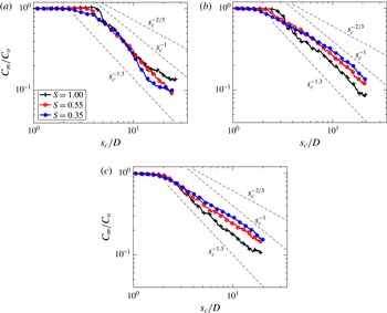
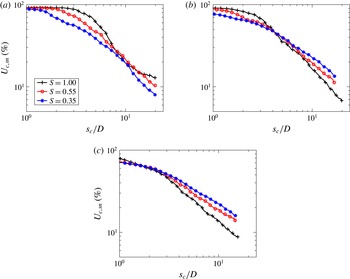
Maximum mean concentration decay as a function of centreline trajectory coordinate
 $s_{c}/D$
for flush nozzle-injected transverse jets at various density ratios
 $S$
, for (a)
 $J=41$
, (b)
 $J=12$
and (c)
 $J=5$
.

Figure 11 shows the maximum mean concentration decay trends for flush nozzle-injected transverse jets for fixed values of density ratio
 $S=1.0$
, 0.55 and 0.35, and for fixed
 $J=41$
,
 $J=12$
and
 $J=5$
. Since
 $J$
is a constant in each of the plots, simple
 $s_{c}/D$
scaling is employed. As noted previously, all
 $J=5$
data and all
 $S=0.35$
data correspond to absolutely unstable conditions; the other conditions shown correspond either to relatively weak convectively unstable shear layers or, for
 $J=12$
, to situations where the shear layer instability is in the process of strengthening and approaching absolute instability (Getsinger et al.
Reference Getsinger, Hendrickson and Karagozian2012). Interestingly, for both
 $J=41$
and
 $J=12$
, potential core lengths differed for the various density ratios, with
 $S=0.35$
producing the shortest core lengths and with a more gradual transition to concentration decay, consistent with immediate vorticity rollup resulting from an absolutely unstable upstream shear layer (Getsinger et al.
Reference Getsinger, Gevorkyan, Smith and Karagozian2014). The
 $J=5$
jets appeared to have potential core lengths that were independent of density ratio, all with a gradual rather than an abrupt concentration decay, again probably related to the fact that all cases in figure 11(c) represented absolutely unstable shear layers with rapid vorticity rollup. The equidensity jets for
 $J=12$
and
 $J=5$
actually appeared to create a higher rate of concentration decay beyond the potential core than for the lower density ratios, but the opposite trend occurred for
 $J=41$
, where lowering the density ratio to
 $S=0.35$
increased the rate of decay in the near field, and with the presence of a branch point at
 $s_{c}/JD\approx 0.36$
. It should also be noted that no observable branch point was measured in the rate of decay for the
 $S=0.55$
,
 $J=41$
jet. These and additional results (Gevorkyan Reference Gevorkyan2015) suggested that, when the transverse jet’s momentum flux ratio was relatively high, e.g.
 $J=41$
, reducing the density ratio and creating an absolutely unstable shear layer appeared to improve mixing, that is, it increased the rate of centreline concentration decay. If one considers that a high momentum flux ratio jet behaves similarly to a free jet in the potential core region, and the fact that lowering the density ratio is observed in recent JICF experiments (Getsinger et al.
Reference Getsinger, Gevorkyan, Smith and Karagozian2014) to create stronger and more coherent periodic shear layer vorticity rollup, as with free jets (Jendoubi & Strykowski Reference Jendoubi and Strykowski1994; Srinivasan, Hallberg & Strykowski Reference Srinivasan, Hallberg and Strykowski2010), an improvement in mixing with lowered density ratio, as seen in figure 11(a), may not be unexpected in the near field. On the other hand, when the momentum flux ratio of the transverse jet was relatively low (e.g.
 $J=5$
), with absolutely unstable shear layers irrespective of density ratio, reducing
 $S$
actually was observed to reduce the rate of concentration decay and possibly worsen mixing. This issue will be explored in the context of other mixing metrics as well as the nature of shear layer vorticity in subsequent sections.
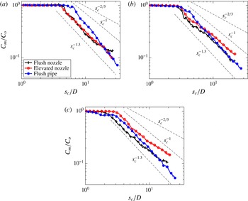
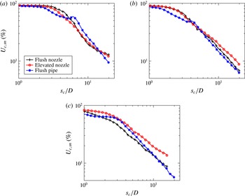
Maximum mean concentration decay as a function of scalar centreline trajectory coordinate
 $s_{c}/D$
for equidensity transverse jets injected from the flush nozzle, elevated nozzle and flush straight pipe injector configurations, for (a)
 $J=41$
, (b)
 $J=12$
and (c)
 $J=5$
.

Figure 12 highlights the explicit effect of different injector configurations on concentration decay for equidensity jets with fixed values of
 $J=41$
,
 $J=12$
and
 $J=5$
. For the high momentum flux ratio,
 $J=41$
case (figure 12
a), the elevated nozzle- and flush nozzle-injected jets had similar concentration decay trends up to
 $s_{c}/D\approx 7$
, with similar potential core lengths and near-field concentration decay rates between these two cases. This would be expected based on the similar trajectories (figure 8) and shear layer stability characteristics (Megerian et al.
Reference Megerian, Davitian, de B. Alves and Karagozian2007; Getsinger et al.
Reference Getsinger, Gevorkyan, Smith and Karagozian2014) for these nozzles at
 $J=41$
. Interestingly, neither the elevated nozzle nor the flush pipe exhibited branch point behaviour and the subsequent reduction in decay rate found in the flush nozzle data, consistent with the pipe injection studies by Su & Mungal (Reference Su and Mungal2004). The pipe flow-injected
 $J=41$
JICF in fact had a somewhat longer potential core than the nozzle flows, consistent with much weaker upstream shear layer instabilities in this regime (Getsinger et al.
Reference Getsinger, Gevorkyan, Smith and Karagozian2014), but ultimately the jet had a much higher concentration decay rate downstream of the potential core. This trend in the pipe flow data appeared to be present for the lower momentum flux ratio cases as well (figure 12
b,c). For all momentum flux ratios, particularly at
 $J=12$
and 5, the elevated nozzle had the weakest rate of concentration decay of all the injectors, with scaling similar to that of the free jet, proportional to
 $s_{c}^{-1}$
. This scaling was consistent with the elevated jet’s significantly weakened shear layer instabilities due to upstream co-flow at higher cross-flow magnitudes (Megerian et al.
Reference Megerian, Davitian, de B. Alves and Karagozian2007; Getsinger et al.
Reference Getsinger, Gevorkyan, Smith and Karagozian2014).
The present observations on mean centreline concentration decay, based on centreplane PLIF imaging, did not provide a clear correlation with previously determined transverse jet shear layer instabilities or structural characteristics (Getsinger et al.
Reference Getsinger, Gevorkyan, Smith and Karagozian2014). Figure 10 indicates that the strongest rate of maximum concentration decay tended to occur for high
 $J$
values and convectively unstable shear layers, especially for flush injection where the jet cross-section has been shown to be asymmetric. Yet in figure 11, data for
 $J=41$
suggested improved concentration decay rates could be attained by lowering the density ratio and hence approaching absolutely unstable conditions which create a more rapid shear layer vortex rollup and, correspondingly, a symmetric CVP in the cross-section. While the nature of entrainment of cross-flow by a jet is clearly dependent on density differences and the formation and evolution of shear layer vortical structures, understanding the precise correlations with mixing requires exploration of additional metrics.
4.3. Cross-section-based mixing metrics
Both cross-sectional (
 $y{-}z$
plane) and centreplane (
 $x{-}z$
plane) based unmixedness
 $U$
may be evaluated from PLIF data scalable to local jet fluid concentration; the same may be said for the averaged spatial p.d.f. metric. For cross-sectional statistics, matching of the mean scaled concentration
 $\overline{C}/C_{o}$
over the
 $y{-}z$
imaging plane at a given
 $x$
location is required to enable comparisons among different operating conditions, as described in § 3. The question of which reference mean value to use for these cross-sectional imaging statistics was explored in detail in the present studies. Two extremes in the selection of the reference
 $\overline{C}/C_{o}$
, for example, could involve the highest (
 $J=41$
) and lowest (
 $J=2$
) momentum flux ratio conditions at the farthest downstream cross-sectional location analysed here,
 $x/D=10.5$
. Figure 13 shows the cross-section-based unmixedness evaluated over the
 $y{-}z$
cross-sectional plane,
 $U_{yz}$
, for the equidensity, flush nozzle-injected transverse jet, where cross-sectional images acquired at three distinct
 $x$
locations were analysed and then plotted as a function of the spatial coordinate
 $s_{c}/D$
, per trajectory data such as those in figure 9. The cross-section-based
 $U_{yz}$
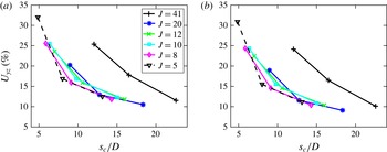
was quantified in two different ways in figure 13. One (figure 13
a) involved matching each instantaneous image’s spatial mean at the given flow condition to a reference mean value corresponding to
 $J=2$
at
 $x/D=10.5$
. Figure 13(b) shows the same information for
 $U_{yz}$
, but with the reference mean value selected to correspond to
 $J=41$
at
 $x/D=10.5$
. Such
 $\overline{C}/C_{o}$
matching was achieved by adding or removing zero-valued pixels to the chosen interrogation area
 $A_{i}$
containing mixed jet fluid. Very little sensitivity of
 $U_{yz}$
values was observed for these two extremes in the mean reference value, despite the fact that the high momentum flux ratio jet had still not turned completely to the horizontal by
 $x/D=10.5$
. Similar observations were made for cross-section-based p.d.f. data (Gevorkyan Reference Gevorkyan2015). All subsequent cross-section-based unmixedness and p.d.f. calculations were thus chosen to employ the mean value of the equidensity, flush nozzle-injected
 $J=2$
JICF at
 $x/D=10.5$
as the reference value for
 $\overline{C}/C_{o}$
; the interrogation areas were adjusted accordingly to match that reference mean.
Cross-sectional (constant
 $x/D$
) based unmixedness,
 $U_{yz}$
, for equidensity flush nozzle-injected transverse jets, plotted against the scalar centreline coordinate
 $s_{c}/D$
. The value of
 $U_{yz}$
was calculated by matching each instantaneous image’s spatial mean to the spatial mean value of the temporal mean image at
 $x/D=10.5$
for two different flow conditions: (a)
 $J=2$
and (b)
 $J=41$
. Results are shown for various momentum flux ratios.

As noted in § 3, the averaged spatial p.d.f.s of jet cross-sectional scalar concentration data can determine local mixing efficiency (Shan & Dimotakis Reference Shan and Dimotakis2006). Cross-section-based spatial p.d.f.s at three different downstream locations (
 $x/D=2.5$
, 5.5 and 10.5) for the equidensity flush nozzle-injected JICF are shown in figure 14(a–c). Cross-sectional p.d.f.s (and unmixedness at the same three values of
 $x/D$
, shown in figure 14
d) were calculated by matching each instantaneous image spatial mean to the spatial mean value of
 $\overline{C}/C_{o}$
as described above. Increased levels of mixing typically result in the appearance of a preferred (most probable) value of the scalar concentration, and an evolution of that preferred value towards the mean. Note that here and in subsequent p.d.f. datasets, p.d.f. data point markers do not represent the actual resolution of data, which is much finer than shown. Unsurprisingly, the p.d.f. data for each
 $J$
value in figure 14(a–c) suggested improved mixing with downstream distance
 $x$
, where, especially for lower
 $J$
values (5 and 2), there was an increase in the magnitude of the p.d.f. and a reduction in the concentration
 $C/C_{o}$
associated with that peak as downstream distance
 $x$
increased. These trends were similarly observed at all
 $J$
values, but the spatial variation in distributions at higher
 $J$
were not as significant as for lower
 $J$
. These overall trends for spatial variation in mixing with
 $J$
variation were also observed in the constant
 $x/D$
based cross-sectional unmixedness,
 $U_{yz}$
, plotted as a function of
 $x/D$
for all three downstream locations in figure 14(d). As with trends in the p.d.f., the degree of reduction in
 $U_{yz}$
with increasing
 $x/D$
was more significant for the lower
 $J$
values than for the larger
 $J$
values. Yet for both p.d.f. and
 $U_{yz}$
cross-section-based metrics plotted as a function of
 $x$
(and not distance along the jet trajectory
 $s_{c}$
), the relatively high
 $J=20$
equidensity flush nozzle JICF provided the ‘best’ local degree of mixing (i.e. the largest peak in the p.d.f. or the lowest value of
 $U_{yz}$
at a given
 $x/D$
location) as compared with other
 $J$
conditions. This
 $J=20$
condition is documented in Getsinger et al. (Reference Getsinger, Gevorkyan, Smith and Karagozian2014) to have a somewhat asymmetric cross-sectional CVP structure, with unequal distributions of jet fluid between the lobes of the CVP, although the degree of asymmetry is not as severe as for
 $J=41$
for this injector, which appeared in figure 14 not to mix as well. The
 $J=20$
condition was not observed to produce the most rapid centreline concentration decay when plotted against
 $s_{c}/D$
, however, per figure 10. Differences in interpretation of mixing data based on parametric variation will be expanded upon below.
Cross-sectional (constant
 $x/D$
) based spatial p.d.f. and unmixedness
 $U_{yz}$
for
 $S=1.00$
transverse jets injected from the flush nozzle injector: (a) p.d.f.,
 $x/D=2.5$
; (b) p.d.f.,
 $x/D=5.5$
; (c) p.d.f.,
 $x/D=10.5$
; and (d) unmixedness
 $U_{yz}$
. Data are shown for various momentum flux ratios.

Figure 15(a–c) provides additional p.d.f. data from cross-sectional slices at the fixed downstream location
 $x/D=10.5$
for
 $J=41$
, 12 and 5, respectively, and for different density ratio values (
 $1.0\geqslant S\geqslant 0.35$
). Figure 15(d) provides comparative data, also extracted from cross-sectional imaging, for the constant
 $x$
based
 $U_{yz}$
as a function of density ratio
 $S$
. There was again considerable consistency between the p.d.f. and
 $U_{yz}$
metrics computed on the basis of a fixed downstream distance
 $x/D$
. Both metrics suggested that, irrespective of momentum flux ratio, at constant downstream position
 $x/D=10.5$
, reducing the jet density relative to the cross-flow at constant
 $Re_{j}$
actually worsened mixing at a given downstream location
 $x$
, especially at the lower
 $J$
values. Mixing (quantified via p.d.f. or
 $U_{yz}$
) for the
 $J=41$
JICF did not change as significantly with a variation in
 $S$
, although, when compared with other density ratios, the equidensity JICF overall seemed to produce slightly better mixing (i.e. a sharper and lower peak in the p.d.f. and a lower overall
 $U_{yz}$
) than for low-density jets.
Cross-sectional (constant
 $x/D=10.5$
) based metrics: (a–c) spatial p.d.f. and (d) unmixedness
 $U_{yz}$
for flush nozzle-injected transverse jets with density ratios
 $S=1.00$
,
 $S=0.55$
and
 $S=0.35$
. Data are shown for various momentum flux ratios: (a) p.d.f.,
 $J=41$
; (b) p.d.f.,
 $J=12$
; (c) p.d.f.,
 $J=5$
; and (d)
 $U_{yz}$
versus
 $S$
for various
 $J$
values.

Yet variation in cross-section-based mixing metrics with scaled downstream distance
 $x/D$
showed different trends when compared with variation in these metrics along the jet centreline,
 $s_{c}/D$
. Because
 $J$
varies significantly among the different cases explored, the value of the centreline distance
 $s_{c}$
can be quite different for the same downstream location
 $x$
. For direct comparison, note that figure 13(a) shows the cross-section-based (constant
 $x/D$
) unmixedness
 $U_{yz}$
for the equidensity, flush nozzle-injected JICF plotted against the scalar centreline trajectory coordinate
 $s_{c}/D$
, while figure 14(d) shows the same parameter plotted as a function of the
 $x/D$
position at which the cross-sectional imaging took place, all with variable
 $J$
values. Note that data for
 $J=2$
in figure 14(d) are not plotted in figure 13(a) because of the inadequacy of the previously noted trajectory fits at this very low momentum flux ratio. While the values of
 $U_{yz}$
in each plot otherwise correspond to the same datasets, the fact that
 $s_{c}$
was considerably larger than
 $x$
at the higher momentum flux ratio conditions, due to much greater jet penetration, completely altered the comparative spatial evolution of the
 $U_{yz}$
metric (and, similarly, p.d.f.s).
These differences in results based on spatial scaling raise a number of questions pertaining to which equidensity JICF flow conditions (e.g.
 $J$
) produce ‘better mixing’. Knowledge of the degree of jet cross-sectional mixing at a specified location
 $x$
downstream of injection could be useful in many practical applications, as is knowing the momentum flux ratio
 $J$
required to achieve a desired level of mixing at a specific downstream location. On the other hand, a fundamental understanding of molecular mixing efficiency by the transverse jet requires mixing quantification as the jet fluid is spatially exposed to cross-flow, particularly when one considers a comparison of molecular mixing by the jet in cross-flow with that for the free jet, where distance along the jet centreline or jet shear layer represents spatial evolution (Smith & Mungal Reference Smith and Mungal1998). This issue pertains to jet cross-section-based metrics as well as to centreplane-based metrics. Given the interest in a fundamental understanding of molecular mixing for the transverse jet as compared with other canonical jet flows, variation of mixing metrics with distance along the jet,
 $s_{c}/D$
, will be examined in the remainder of this paper.
4.4. Comparison of centreplane- and cross-section-based unmixedness
For jet centreplane (
 $x{-}z$
) based mixing statistics, matching of the mean scaled concentration
 $\overline{C}/C_{o}$
over the relevant interrogation area was similarly required to enable comparisons among different operating conditions, as discussed for cross-sectional mixing metrics in §§ 3 and 4.3. Concentration values and associated local mixing metrics could be evaluated over narrow slices of the jet oriented in the jet-normal direction
 $n$
, with a fixed interrogation area width in the
 $s_{c}$
direction, as shown in figure 6(b). For such an interrogation area, the local centreplane-based unmixedness is designated
 $U_{c,sn}$
. Alternatively, one could explore centreplane-based mixing metrics such as unmixedness evaluated over comparably narrow vertical slices of the jet, but with a fixed width in the
 $x$
direction and extending vertically in the
 $z$
direction; this centreplane-based unmixedness is designated
 $U_{c,xz}$
. For a very thin interrogation area,
 $U_{c,xz}$
could be compared with the cross-section-based unmixedness
 $U_{yz}$
obtained at the same average downstream location
 $x$
. Recall that cross-section-based metrics were calculated by matching each instantaneous image’s spatial mean to the spatial mean value,
 $\overline{C}/C_{o}$
, for the temporally averaged cross-sectional image at
 $x/D=10.5$
for the flush nozzle-injected, equidensity,
 $J=2$
case. Centreplane-based metrics were calculated by matching each interrogation area’s spatial mean to the spatial mean of the temporally averaged concentration at the location
 $s_{c}/D=15$
corresponding to the flush nozzle-injected, equidensity,
 $J=5$
case. This condition was chosen because trajectory quantification was more difficult for
 $J=2$
. As with cross-section-based metrics, the centreplane-based metrics did not change significantly with alterations in the selected matched mean value of
 $\overline{C}/C_{o}$
for different operating conditions (Gevorkyan Reference Gevorkyan2015).
Figure 16(a,b) displays centreplane-based unmixedness variation along the jet trajectory, for the equidensity transverse jet injected from the flush nozzle at a range of momentum flux ratios. Here one can compare trends in local centreplane
 $U_{c,xz}$
based on a thin (seven-pixel-wide) interrogation area oriented in the
 $x{-}z$
direction (figure 16
a) and local centreplane unmixedness
 $U_{c,sn}$
based on a seven-pixel-wide interrogation area oriented in the
 $s_{c}{-}n$
direction (figure 16
b). The former may be compared with cross-sectional unmixedness
 $U_{yz}$
measured at three different downstream locations, shown in figure 13(a). All data here are plotted as a function of
 $s_{c}/D$
. Interestingly, the two centreplane-based metrics in figure 16(a,b) showed few differences in the evolution of mixing, the exception being at
 $J=30$
, with a somewhat greater degree of unmixedness reduction in
 $U_{c,sn}$
as compared with
 $U_{c,xz}$
. Figure 16(a,b) also shows very similar trends to the variation in cross-section-based unmixedness,
 $U_{yz}$
, in figure 13(a). Note that the
 $J=30$
case produced such severely asymmetric mean jet cross-sections for the flush nozzle that it was not possible to accurately scale the cross-sectional concentration data with respect to the centreplane concentration data. Hence no comparable quantitative cross-section-based data for this case are shown in figure 13, for example. All three plots (figures 13
a and 16
a,b) demonstrated that, generally speaking, lower local momentum flux ratio transverse jets produced lower centreplane-based and cross-section-based values of unmixedness, at least until around 20 diameters along the jet trajectory. The rate of decay in unmixedness did appear to be greater for
 $J=30$
and 20 for the near-field region as compared with other conditions. Nevertheless, jets whose upstream shear layers have been documented to be absolutely unstable (Megerian et al.
Reference Megerian, Davitian, de B. Alves and Karagozian2007), with
 $J=8$
and 5, appeared to have the best overall mixing characteristics, although this advantage diminished further along the jet, near
 $s_{c}/D=20$
. Data for
 $J=41$
appeared to have the worst overall mixing characteristics, yet similar to the
 $J=30$
JICF, there was significant asymmetry in the
 $J=41$
jet’s mean cross-sectional shape (Getsinger et al.
Reference Getsinger, Gevorkyan, Smith and Karagozian2014), which probably affected these trends.
For the flush nozzle-injected, equidensity JICF, (a) centreplane unmixedness
 $U_{c,xz}$
based on a thin interrogation area oriented in the
 $x{-}z$
direction and (b) centreplane unmixedness
 $U_{c,sn}$
based on a thin interrogation area oriented in the
 $s_{c}{-}n$
direction. Each is plotted as a function of
 $s_{c}/D$
for various momentum flux ratios
 $J$
.

There were similar trends in the comparison between centreplane-based unmixedness
 $U_{c,xz}$
and cross-section-based
 $U_{yz}$
for other injectors, as well as for a given injector at reduced density ratios. Such comparisons are most logical given that the laser sheet for cross-sectional mixing metrics always lies in the
 $y{-}z$
plane. For example, figure 17 shows constant
 $x/D$
based centreline unmixedness
 $U_{c,xz}$
(a,b) as well as cross-section-based
 $U_{yz}$
(c,d) as a function of distance along the jet trajectory, for the elevated nozzle (a,c) and flush pipe (b,d). Data here correspond to the equidensity JICF. As with the flush nozzle (figures 16
a and 13
a), the effects of momentum flux ratio on spatial variation in
 $U_{c,xz}$
were very similar to those for spatial variation in
 $U_{yz}$
. At a given scaled distance along the jet trajectory,
 $s_{c}/D$
, higher momentum flux ratio jets (
 $J\geqslant 20$
) tended to mix less well than did the JICF at lower
 $J$
, even when these lower-
 $J$
conditions did not produce an absolutely unstable shear layer, as was the case for the elevated nozzle. When the upstream shear layer did become absolutely unstable, however, as was the case for the flush nozzle and flush pipe for
 $J\lesssim 12$
, the actual values of unmixedness at a given location
 $s_{c}/D$
tended to be lower than for the more weakly unstable elevated jets at the same flow conditions. Datasets missing in these plots, e.g.
 $J=30$
and
 $J=41$
for the flush pipe’s cross-sectional statistics, were the result of cross-sectional asymmetries that prohibited an accurate determination of local jet concentration.
Centreplane unmixedness
 $U_{c,xz}$
based on a thin interrogation area oriented in the
 $x{-}z$
direction (a,b) and cross-sectional unmixedness
 $U_{yz}$
(c,d), both plotted as a function of
 $s_{c}/D$
for equidensity transverse jets of various momentum flux ratios. Shown are data for (a,c) the elevated nozzle and (b,d) the flush straight pipe injector.

Centreplane unmixedness
 $U_{c,sn}$
plotted as a function of
 $s_{c}/D$
on a log–log plot. Data are shown for the equidensity JICF for various momentum flux ratios
 $J$
, injected from (a) the flush nozzle, (b) the elevated nozzle and (c) the flush pipe.

Trends in local centreplane-based unmixedness
 $U_{c,sn}$
, extracted from a thin interrogation area oriented in the
 $s_{c}{-}n$
direction, may be compared with the more traditional maximum centreline concentration decay metric shown in figures 10–12. When similarly plotted as a function of
 $s_{c}/D$
and represented on a log–log plot, centreplane-based unmixedness
 $U_{c,sn}$
was generally observed to decay with the same trends as for concentration decay. These unmixedness trends are shown in figures 18–20, which may be compared with figures 10(a–c), 11 and 12, respectively. The general trends in the effects of
 $J$
,
 $S$
and injector type on mixing, as represented by both relative metric values and by the spatial rate of decay of the metric, were very similar between
 $C_{m}/C_{o}$
and
 $U_{c,sn}$
, although with a few important differences. For example, for the equidensity, flush-nozzle-injected JICF with variable
 $J$
, as examined in both figures 18(a) and 10(a), the lowest centreline concentration and unmixedness cases at a given location
 $s_{c}/D$
corresponded to those for low
 $J$
and, in general, an absolutely unstable upstream shear layer. When the rate of decay of the metric beyond the potential core is considered, however, both
 $J=30$
and 20 tended to produce the largest reduction, seen in both metrics. Similar correspondence in spatial evolution between
 $C_{m}/C_{o}$
and
 $U_{c,sn}$
was observed when density ratio
 $S$
was reduced for the
 $J=41$
flush nozzle, as shown in figures 19(a) and 11(a), and for a worsening in mixing for the
 $J=5$
flush nozzle, shown in figures 19(c) and 11(c). The effects of injector configuration on mixing metrics quantified in figures 12 and 20 had similar correspondence with one another. One striking difference between the
 $C_{m}/C_{o}$
and
 $U_{c,sn}$
metrics, however, was the much less sharp delineation of the potential core and subsequent drop-off in
 $U_{c,sn}$
as compared with
 $C_{m}/C_{o}$
, particularly under conditions corresponding to absolutely unstable shear layers. This difference clearly resulted from the nature of a centreline-based metric, for which only potential core fluid is quantified immediately after injection, as compared with a metric such as
 $U_{c,sn}$
(or other centreplane-based statistical metrics), which accounts for the distribution of the scalar field across the span of the jet, thus including the effects of near-field shear layer distortion more explicitly.
Centreplane unmixedness
 $U_{c,sn}$
plotted as a function of
 $s_{c}/D$
on a log–log plot. Data are shown for flush nozzle-injected transverse jets of various density ratios
 $S$
, with momentum flux ratios (a)
 $J=41$
, (b)
 $J=12$
and (c)
 $J=5$
.

Centreplane unmixedness
 $U_{c,sn}$
plotted as a function of
 $s_{c}/D$
on a log–log plot. Data are shown for the equidensity JICF with the flush nozzle, elevated nozzle and flush straight pipe injectors, for momentum flux ratios (a)
 $J=41$
, (b)
 $J=12$
and (c)
 $J=5$
.

4.5. Interpretation of mixing trends
Finally, it is of interest to explore the possible physical phenomena behind some of the mixing trends observed here. For low momentum flux ratios
 $J$
, as noted, reducing the density ratio
 $S$
actually worsened molecular mixing, e.g. for
 $J=5$
in figures 11(c), 15(c,d) and 19(c). In contrast, at higher
 $J$
values, reducing the density ratio from
 $S=1.0$
to
 $S=0.35$
appeared to improve mixing, as suggested for
 $J=41$
in figures 11(a) and 19(a), or at least not to alter the mixing very significantly, as suggested in figure 15(a,d). Data for transitional momentum flux ratios, e.g. for
 $J=12$
in figures 11(b), 15(b,d) and 19(b), appeared to be more similar to
 $J=5$
and other low momentum flux ratio cases. The upstream shear layer for
 $J=5$
conditions has been documented to be absolutely unstable for all density ratios, while only the
 $S=0.35$
conditions clearly produce absolutely unstable shear layers at
 $J=41$
and 12, although the latter case involved much stronger convective instabilities than at higher
 $J$
(Getsinger et al.
Reference Getsinger, Gevorkyan, Smith and Karagozian2014). These differences in the instabilities and the implications for vorticity rollup may be observed in high-resolution instantaneous centreplane images shown in figure 21 for this range of
 $J$
values, for equidensity and low-density (
 $S=0.35$
) conditions. As documented in Getsinger et al. (Reference Getsinger, Gevorkyan, Smith and Karagozian2014), all absolutely unstable shear layer conditions produced immediate or near-immediate upstream vorticity rollup; for convectively unstable conditions, the initial rollup is weaker and delayed to a location further along the shear layer. For the equidensity JICF, however, shear layer rollup appeared to draw in considerably more cross-flow fluid (of a lower scalar concentration) into the vortical structures than did the low-density JICF, irrespective of
 $J$
value. The
 $S=0.35$
images all showed shear layer vortices comprised largely of low-density jet fluid, and this clearly influenced mixing parameters when the span of the jet (either in the jet-normal direction
 $n$
or in the cross-sectional plane,
 $y{-}z$
) was used in mixing metric quantification. Even the centreline-based metric in figure 11 captured this trend, because of the influence of the shear layer vortices on the potential core. The reduction in entrainment of higher-density fluid into a lower-density vortical structure has been seen in a number of prior reactive shear layer studies, both experimental (Hermanson, Mungal & Dimotakis Reference Hermanson, Mungal and Dimotakis1987; Hasselbrink & Mungal Reference Hasselbrink and Mungal2001) and computational (Karagozian & Marble Reference Karagozian and Marble1986).
Instantaneous high-resolution centreplane (side view) acetone PLIF imaging of the flush nozzle-generated JICF with: (a)
 $J=41$
and density ratio
 $S=1.0$
; (b)
 $J=41$
and density ratio
 $S=0.35$
; (c)
 $J=12$
and density ratio
 $S=1.0$
; (d)
 $J=12$
and density ratio
 $S=0.35$
; (e)
 $J=5$
and density ratio
 $S=1.0$
; and (f)
 $J=5$
and density ratio
 $S=0.35$
.

Figure 21 further demonstrates that, for a relatively weak convectively unstable shear layer, as for the equidensity JICF with
 $J=41$
in figure 21(a), accelerating vorticity rollup by creating an absolutely unstable shear layer (figure 21
b) did appear to improve mixing. But when the upstream shear layer instability was already relatively strong and closer to being absolutely unstable (as for the equidensity
 $J=12$
condition in figure 21
c), reducing the jet density and creating the absolute instability did not have a significant benefit for mixing, probably due to the reduced local entrainment of cross-flow observed in figure 21(d). It is also noted that the sizes of the vortical structures in figure 21 were not significantly altered by the alteration in density ratio, consistent with the observations of Brown & Roshko (Reference Brown and Roshko1974) on the relatively weak effect of density ratio alone in actual shear layer growth. Yet the entrainment of higher-density fluid from the cross-flow into the lower-density vortical structures did appear to affect near-field and eventually far-field mixing quantification.
Differences in mixing metrics between the flush nozzle- and flush pipe-injected equidensity JICF (e.g. in figures 12, 16
a, 17
b,d and 20), especially in the near field of the jet, may also be explained based on instantaneous centreplane images. Figure 22(a–c) corresponds to instantaneous PLIF images for the equidensity flush pipe at
 $J$
values of 41, 12 and 5, respectively, and may be compared with flush nozzle-generated images in figure 21(a,c,e). Additional centreplane (and cross-sectional) images comparing equidensity flush nozzle and pipe flows may be found in Getsinger et al. (Reference Getsinger, Gevorkyan, Smith and Karagozian2014). While the weaker shear layer instabilities for the flush pipe at higher
 $J$
were manifested in delayed and larger, less coherent vortices in the upstream shear layer as compared with those for the flush nozzle, the greater distortion of jet fluid upon exit into the cross-flow when momentum flux ratio was reduced, especially at
 $J=5$
, did appear to affect jet mixing by the pipe injector, especially in the near field. These mixing differences between flush pipe and nozzle configurations did seem to switch beyond the first few diameters along the
 $J=5$
jet trajectory, however (e.g. as seen in figure 20
c), so trends in absolutely unstable JICF conditions for different injectors also did not follow more straightforward trends seen for convectively unstable jet conditions.
Instantaneous high-resolution centreplane (side view) acetone PLIF imaging of the flush pipe-generated, equidensity JICF with: (a)
 $J=41$
, (b)
 $J=12$
and (c)
 $J=5$
.

5. Conclusions
The present experimental studies of scalar concentration evolution and mixing quantification for the equidensity and low-density jet in cross-flow provide new insights into molecular mixing trends and underlying physical phenomena, as well as differences in the ways mixing metrics can be interpreted. When unmixedness or p.d.f. metrics were plotted as a function of scaled downstream location
 $x/D$
, as opposed to plotting the same metric as a function of scaled distance along the jet concentration centreline trajectory,
 $s_{c}/D$
, different conclusions could be derived with respect to the flow conditions creating the ‘best’ degree of molecular mixing. Figure 13(a), for example, suggests that lower momentum flux ratio jets, typically with absolutely unstable shear layers, had the lowest values and most rapid near-field rate of decay in cross-sectional unmixedness
 $U_{yz}$
, when plotted as a function of
 $s_{c}/D$
, while figure 14 suggests that, at given downstream locations
 $x/D$
, the
 $J=20$
condition produced the ‘best’ mixed jet as compared with other
 $J$
values. Yet the latter type of scaling did not account for the fact that, at a given
 $x$
location, the (flow) ‘time’ of exposure of the jet to the cross-flow fluid was considerably longer for large
 $J$
values than for small
 $J$
values, where the jet turns more abruptly after injection. Given that the
 $s_{c}/D$
scaling expresses the spatial evolutionary aspects of mixing along the jet trajectory, analogous to that for the free jet, and thus is more appropriate for comparisons for different
 $J$
values, the present study has focused on
 $s_{c}/D$
based scaling, although it is noted that
 $x/D$
scaling could be of use in a number of practical applications.
Another observation on mixing metrics for the JICF was that there were very similar trends and parameter values in the comparison between centreplane-based unmixedness
 $U_{c,xz}$
(quantified by a narrow interrogation strip in the
 $x{-}z$
plane) and the cross-section-based
 $U_{yz}$
at the same trajectory location
 $s_{c}/D$
. This remarkable correspondence was observed for all injectors studied here, as well as for a given injector at reduced density ratios. Trends in maximum centreline concentration decay
 $C_{m}/C_{o}$
and centreplane unmixedness
 $U_{c,sn}$
were also reasonably close to one another, although important differences in the local mixing in the vicinity of the exit plane/potential core, arising from strong shear layer vorticity for absolutely unstable jets, were only measurable in the latter metric. It is noted, however, that both
 $C_{m}/C_{o}$
and
 $U_{c,sn}$
displayed a ‘crossing over’ of decay lines for varying
 $J$
in the equidensity flush nozzle (figures 10
a and 18
a), a phenomenon that Smith & Mungal (Reference Smith and Mungal1998) suggest is responsible for flame or other reaction length minima under specific flow conditions.
The question of which flow and geometrical conditions (
 $J$
,
 $S$
,
 $Re_{j}$
, injector shape) produced the ‘best’ mixed jet in cross-flow is further dependent on how one examines the variation in the mixing metric with distance
 $s_{c}/D$
along the jet trajectory. For the equidensity JICF, the flush pipe appeared to have a more rapid rate of unmixedness decay along the jet centreline (hence a ‘better’ mixing rate) than that for the other injectors shown in figure 20, for the range of
 $J$
values explored here,
 $5\leqslant J\leqslant 41$
. The flush nozzle itself, which has been the subject of more extensive study by our group and others, had a more rapid decay in unmixedness (figure 18
a) at specific momentum flux ratios
 $J=30$
and 20), while the rates of unmixedness decay for the lower-
 $J$
jets with stronger shear layer rollup, including absolutely unstable shear layers, were not as large.
The actual value of the mixing metric, however, contains information on the degree of entrainment of cross-flow into the jet fluid as well as statistical information on the level of mixing progress at that location, which is an integral function of the mixing rate. When using the actual value of
 $U$
as a measure of mixing in the equidensity JICF, plotted as a function of
 $s_{c}/D$
, nearly all results in the present study suggested that jets with absolutely unstable upstream shear layers, at relative low
 $J$
values, had greater local mixing at a given
 $s_{c}$
location than did jets with higher
 $J$
. This is consistent with the increased near-field jet-to-cross-flow interfacial area generation caused by the vortex roll-up. These trends were observed for both the flush nozzle and flush pipe; the elevated nozzle did not produce jets with strong upstream shear layer instabilities in this flow range, but nevertheless produced slightly improved mixing for lower
 $J$
conditions.
Mixing trends for the transverse jet at reduced density ratios
 $S$
, for a fixed jet Reynolds number and fixed
 $J$
, produced differing and somewhat unexpected trends. At higher momentum flux ratios, e.g.
 $J=41$
in figure 19, lowering the jet’s density relative to that of the cross-flow appeared to improve molecular mixing at given
 $s_{c}$
locations, although the rate of decay of the equidensity jet appeared to be greater for a narrow range of distances along the jet. Yet for lower
 $J$
values, especially the absolutely unstable
 $J=5$
condition, lowering the density ratio actually appeared to increase the unmixedness, and thus worsen mixing as compared with the equidensity condition. These observations were determined to result from differences in the nature of entrainment of high-density fluid into shear layer vortices by a lower-density jet, as shown in figure 21. Hence even if the shear layer rollup for the JICF was rapidly initiated, as for absolutely unstable conditions, the nature of the fluid contained within the vortical structures has a significant influence on the quantification of mixing, in both the centreplane view and the cross-sectional view.
The present studies provide a great many new insights into the structure and mixing characteristics for the jet in cross-flow, with substantial evidence for a correspondence among jet shear layer instabilities, cross-flow entrainment, and jet mixing and trajectories. It should be noted that, in an experimental mixing study such as this, it is often difficult or impossible to control all the pertinent variables that could affect the mixing efficiency of the flow field. Yet there is a theoretical basis for the assertion that increased instability near the jet exit enhances mixing. Owing to the diffusion-limited mixing processes in this flow field, any changes in the flow that promote diffusion will increase mixing. Instability in the shear layer near the jet exit has been shown to enhance diffusion by increasing interfacial area and concentration gradients between the jet and the cross-flow. The reader should bear in mind, however, that a fully turbulent jet in cross-flow has scales of convection that are not relevant to the present flow field, and thus may behave differently when parameters such as
 $J$
or
 $S$
are varied. Nevertheless, for the diffusion-limited mixing processes explored here, the present studies reaffirm the notion that an understanding of the nature of jet instabilities and structure can provide strategies for optimizing conditions producing well-mixed jets, but also go further to suggest that jet exit conditions (velocity profile, density, acceleration of shear layer vorticity rollup) play a key role in affecting such mixing. Hence, as observed in recent studies on jet excitation (Davitian et al.
Reference Davitian, Hendrickson, Getsinger, M’Closkey and Karagozian2010b
), jet excitation strategies may be developed to enable temporal and spatial tailoring of the flow at the jet exit to create near-field and far-field mixing improvement. Such tailored excitation is the subject of ongoing study for this flow field.
Acknowledgements
The authors thank Professor L. Cortelezzi of McGill University and Professor I. Mezic of University of California, Santa Barbara, for helpful discussions on alternative mixing metrics, and W. Y. Peng and A. Besnard for assistance during the course of these experiments. This project has been supported by the National Science Foundation under grants CBET-1133015 and CBET-1437014, and by the Air Force Office of Scientific Research under grant FA9550-11-1-0128 and DURIP grant FA9550-10-1-0461.