

Background
ERM has many definitions. The generally agreed concept is that ERM is wider than traditional risk management and covers all the risks within an enterprise (or company). Traditional risk management focuses on identifying risks, measuring and monitoring risks and designing strategies to limit losses to agreed limits. ERM recognises that businesses take risks in order to make a profit for their owners and therefore considers the upside of taking risks, and attempts to strike a balance between too much risk and not enough risk compared to the enterprise's strategic direction. Risk is managed holistically in a fully integrated framework, across all different risk types and the different functions/companies within the organisation.
The Call For Research
The Profession invited proposals on a number of topics, which included the following areas:
1. How should firms define and use “risk appetite”, but with the emphasis on the need that outputs should be practically grounded and expressed.
2. How should firms identify and assess the hard to define risks – what techniques are available and how do they work in practice? This topic could possibly be linked with practical techniques for reporting on emerging risk and strategic risks, to mirror text from the recent Walker Report.
This research was awarded to Milliman and the Universities of Bristol and Bath Systems Centre.
The Research
Traditional approaches to risk studies and risk management are based upon the paradigm of risk as an event adequately characterised by a single feature. This simplistic conceptualisation of risk leads to the use of analysis tools and models which do not reliably integrate qualitative and quantitative information or model the interconnectivity of the dynamic behaviour of risks. For complex systems, like an economy or financial organisations, a new paradigm or philosophy is required to understand how the constituent parts interact to create behaviours not predictable from the ‘sum of the parts’. Systems theory provides a more robust conceptual framework which views risk as an emerging property arising from the complex and adaptive interactions which occur within companies, sectors and economies.
Risk appetite is a concept that many practitioners find confusing and hard to implement. The fundamental problem is that there is no common measure for all risks, and it is not always clear how different risk factors should be limited in order to remain within an overall “appetite”. Attempts are generally made to force everything into an impact on profit or capital but this is problematic when businesses and risk decisions become more complex. There is a lack of real understanding about how they would propagate, or indeed how the appetite may shift or evolve to have a preference for specific risks.
By thinking holistically, risk appetite can be viewed as “our comfort and preference for accepting a series of interconnected uncertainties related to achieving our strategic goals”. By making those uncertainties and the connectivity of the underlying drivers explicit, it is possible for decision makers to define their risk appetite and monitor performance against it more effectively. The ability to link multiple factors back to financial outcomes also makes the challenge of expressing risk appetite in those terms more tractable.
Similarly, the identification and assessment of emerging risks can become more robust by using a systems approach that enables a clearer understanding of the underlying dynamics that exist between the key factors of the risks themselves. It is possible to identify interactions in a system that may propagate hitherto unseen risks. Emerging risks can be viewed as evolving risks from a complex system. It is also known that such systems exhibit signals in advance of an observable change in overall performance. Knowing how to spot and interpret those signs is the key to building a scientific and robust emerging risk process. Also it is becoming increasingly clear that risk appetite and emerging risks are interconnected in many ways, as this research shows.
Risk Appetite
Assuming that strategic goals are already identified, establishing a risk appetite framework comprises two distinct parts, one top down and the other bottom up. First, it is necessary to describe how much uncertainty about the achievement of specific business goals is acceptable, and what the key sources of that uncertainty are. Second, it is necessary to identify the key operational activities or actions which contribute to each source of uncertainty and then apply the necessary limits to those activities to maintain performance within the desired risk appetite.
Systems techniques used in the case study proved extremely effective at helping businesses to explain their understanding of how uncertainty arises around their business goals. Cognitive mapping was used to elicit a robust understanding of the business dynamics creating uncertainty in business goals. This process was useful for engaging the business and capturing their collective knowledge of the risk appetite problem.
By carrying out a mathematically based analysis on the cognitive maps it is possible to quickly and objectively identify which parts of the description are most important in explaining the uncertainties we are attempting to constrain. It also highlights areas which have not been particularly well described or understood, prompting further discussion and analysis. This provides a hypothesis for our risk appetite, and associated limit, framework.
Bayesian Networks are proposed to provide a dynamic model of how the various risk factors connect and interact. This links the behaviour of the operational activities to the levels of risk they produce and can be parameterised through a combination of qualitative and quantitative data.
Bayesian Networks permit evidence to propagate up and down the model, providing the business with a robust method for determining risk limits by setting the level of risk to be at the risk appetite point and observing what level the limits should be to ensure compliance with this level of risk. Alternatively, the observed indicator values can be entered and the implied level of risk is computed. Making this linkage explicit provides a mechanism for companies to understand more immediately where their risk exposure is coming from and how to control it.
Emerging Risk
There are a number of techniques which can be used from a systems perspective to provide insight into the development of risks and to give earlier warnings of emerging risk. One such technique is described in this research report which uncovers the evolutionary development of risks in a manner which provides structured information about the patterns of that evolution and a way to make sense of apparently unconnected risk factors.
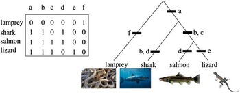
Phylogenetic analysis (a technique developed in the biological sciences) removes subjectivity in risk classification, using evolution as a kind of external reference point. This can be used to provide a methodology that makes clear the data, assumptions and results with the intention of making risk classification decisions transparent. It cuts across organisation boundaries and disciplines and looks at risks for what they are, at an almost fundamental level, and then groups them accordingly. This can be particularly useful for losses, if good loss data about individual losses is available.
Understanding Risk History
Phylogenetics can trace how risks have changed over time. This allows a much deeper understanding of the risks. Risks need no longer be seen as an event occurring now but can instead be understood by the interacting circumstances that have brought the risk into its current form. This allows companies to improve their understanding of vulnerabilities and how to prioritise their risk management resources and to manage their risks better.
Predicting Risk Futures
Phylogenetics provides a way to use the history of risk evolution as an indication of its future evolutionary pathway. Although past corporate behaviour does not ensure the understanding of future outcomes, it provides a guide to major risk factors, and understanding the history of a risk will give glimpses as to its future. By no longer viewing risk as a fixed entity but one that varies over time, a risk's variations can be traced and its future state predicted.
Risk can change and evolve in many ways but this does appear to happen in some predictable ways. Predicting the most likely future of the evolution of a risk will not only allow better risk mitigation but can prevent new risks from forming. From this, risks can be mitigated before they have even been identified as risks.
1. Introduction
1.1 The aim of this study is to apply new thinking and techniques from complex systems science to two key problem areas for risk management and governance identified in the Walker report (Walker, Reference Walker2009):
1. How can firms develop a robust and practical framework for describing their ‘risk appetite’, which also enables appropriate risk limits to be attached to key business drivers and outcomes?
2. How can firms identify “hard to define or emerging risks”, and assess those risks in such a way that the underlying drivers and dynamics can be made transparent and hence included in building quantitative models.
1.2 Traditional approaches to risk studies and risk management are based upon the paradigm of risk as an event adequately characterised by a single feature. This simplistic conceptualisation of risk leads to the use of analysis tools and models which do not reliably integrate qualitative and quantitative information or model the interconnectivity of dynamic behaviour of risks. For complex systems like an economyFootnote 1 or financial organisations a new paradigm or philosophy is required to understand how the constituent parts interact to create behaviours not predictable from the ‘sum of the parts’. Systems theory provides a more robust conceptual framework which views risk as an emerging property arising from the complex and adaptive interactions which occur within companies, sectors and economies.
Systems approach
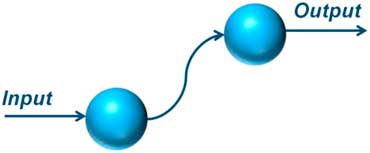
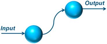
1.3 So what is a system? Essentially it is any two or more elements that are interconnected for a purpose as shown in figure 1.
A basic system directed at a single purpose or outcome
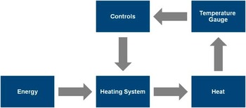
1.4 A system starts to get interesting when we get feedback and interactions with multiple elements connected. For example a system for heating a single room with no windows could be represented by the schematic in figure 2. Energy is added as an input to the central heating system with heat coming out. The heat is controlled by a temperature sensor and a control device. With a simple system, with no external influence, it should be possible for the system to settle down to a nice steady state and keep the room at a constant temperature. However, is the whole room at the same temperature? Where is the temperature gauge? How quickly is the heating system responding to the change? If the control is too sensitive the heating will be switching on and off too rapidly or if not sensitive enough then the room stays too cold or too hot for too long. So what time lag is acceptable, what tolerance is needed and what efficiency is required? These are all important questions transforming this into a not-quite-so-simple system.
A schematic of a simple heating system for a single room

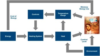
1.5 Now imagine trying to heat a large building that has multiple rooms, windows and doors, and a changing external environment which is sometimes hot and sometimes cold. To make the example a little more realistic, assume that there are people in the rooms who have different needs, feel the temperature differently and think about the cost of energy to a lesser or greater extent. Furthermore, the occupants of the rooms have access to the thermostat so they can send individual signals to the heating system. This more realistic system is shown schematically in figure 3.
A heating system with human intervention

1.6 Clearly the system behaviour has become more uncertain with the introduction of people and their localised decision making. There are now multiple feedback loops and the impact of the changing environment needs to be taken into account. Most importantly, there are multiple objectives which could be competing with each other so some degree of optimisation (or compromise) needs to be reached.
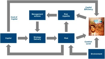
1.7 These issues are also fundamental to the issue of risk appetite and figure 4 attempts to apply the heating analogy to the risk appetite system. Here we have capital as our energy and the implementation of our strategy as the means of turning that into desired business outcomes. To the extent that these goals are not achieved we experience risk, which is analogous to the heat in figure 3. Our risk appetite is an expression of the amount of heat we are comfortable with and we use our management processes to maintain that within acceptable levels. An additional level of complication for many types of firm is that the level of risk they experience also impacts upon the level of capital they have available to control it, so we have an extra feedback loop compared to the heating example.
The heating system analogy applied to a risk appetite system

1.8 Risk appetite is a concept that many practitioners find confusing and hard to implement. The fundamental problem is that there is no common measure for all risks, and it is not always clear how different risk factors should be limited in order to remain within an overall “appetite”.
1.9 Attempts are generally made to force everything into an impact on profit or capital but this is problematic when businesses and risk decisions become more complex. There is a lack of real understanding about how they would propagate, or indeed how the appetite may shift or evolve to have a preference for specific risks. This difficult challenge is shown in figure 5.
Risk appetite is hard due to the many conflicting constraints

1.10 The heating system is a useful analogy for a preliminary understanding of the complex nature of risk appetite. The system starts to show the multitude of interconnections and feedback loops that need to occur in any complex financial organisation. A more complete system model can be based on such a heating system analogy by integrating more real world considerations.
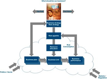
1.11 Figure 6 attempts to build on the understanding of the risk appetite problem from a systems perspective and provides a generic statement of the practitioner's problem. This in turn provides a starting point for how systems thinking may provide useful approaches to tackling the problem of risk appetite, emerging risk and risk management in general. By thinking holistically, risk appetite can be viewed as “our comfort and preference for accepting a series of interconnected uncertainties related to achieving our strategic goals”. By making those uncertainties and the connectivity of the underlying drivers explicit, it is possible for decision makers to define their risk appetite and monitor performance against it more effectively. The ability to link multiple factors back to both financial and non-financial outcomes also makes the challenge of expressing risk appetite in a more complete way more tractable.
A more complete system diagram of risk appetite
In an organisation, it may have multiple business units. The cloud represents the rather fuzzy boundary between the organisation and the business environment, with political and market forces influencing all the elements inside the boundary to a lesser or greater extent. The risk appetite process box is deliberately placed on the boundary as this represents the complex integration of external and internal strategic decisions that needs to be made.

1.12 Similarly, the identification and assessment of emerging risks can become more robust by using a systems approach that enables a clearer understanding of the underlying dynamics that exist between the key factors of the risk system and the risks themselves. It is possible to identify interactions in a system that may propagate hitherto unseen risks. Emerging risks can be viewed as evolving risks from a complex system. It is also known that such systems exhibit signals in advance of an observable change in overall performance. Knowing how to spot and interpret those signs is the key to building a scientific and robust emerging risk process. The early treatment of risk is nearly always more efficient than applying resource to the resolution of crystallised risk event, and so having information about the onset of new risk developments as early as possible affords firms a way to manage their scarce financial and other resource in a robust and effective manner. Also it is becoming increasingly clear that risk appetite and emerging risks are interconnected in many ways which will be developed in the following chapters.
Boundaries to the study
1.13 The focus of the study is on the strategic management level of an enterprise, not at any specific function or industry sector level. Hence risk appetite and emerging risks will be viewed from a strategic perspective within an enterprise, even though multilevel risk interactions across an enterprise are at the heart of these issues. Influences on the enterprise from the outside environment such as market and regulatory changes will be considered in relation to how they might impact on the problem or be necessary for control and monitoring. The tools developed, however, can be applied in an analogous way at lower levels of the organisation to cascade the high level results through organisational layers to achieve a robust and consistent framework.
Structure of the report
Chapter 2 – A brief review of the relevant literature relating to risk appetite from a practitioner's perspective. This forms the basis for matching the systems concepts to the domain specific problem of risk appetite.
Chapter 3 – A brief review of the relevant literature relating to emerging risks from a practitioner's perspective is then presented, including a discussion about systemic risks.
Chapter 4 – In this chapter we give an overview of the key concepts of systems thinking, complex adaptive systems and complexity and how these may specifically relate to the issue of risk appetite and emerging risks.
Chapter 5 – Then a set of tools and techniques from the complexity sciences and systems science are discussed in relation to how useful they might be to the stated problems of risk appetite and emerging risk.
Chapter 6 – Based on a series of research workshops this chapter illustrates how the selected tools have been used when applied to a case study based on data from a life insurer, to trial against a number of real case studies. The methodology, application, analysis, results and conclusions are presented.
Chapter 7 – This chapter is very similar in approach but applies a specific technique to emerging risk to data from a multi-line international insurer. Again the emphasis is on the methodology, analysis, results, interpretation and conclusions. There are also details of appropriate software and different approaches.
Chapter 8 – This is the final chapter before references and the appendices and consolidates the key messages from this research and gives guidance for practitioners on how to begin to tackle the very contemporary questions of risk appetite measurement and how to identify emerging risk.
A full set of references, bibliography, glossary, useful contacts and appendices are included at the end of the report.
2. Overview of the risk appetite concept in ERM
2.1 The latest financial turmoil has caused unprecedented harm to the economy locally and globally. Consequently governments, regulatory bodies, professional associations, as well as financial institutions are working closely to create robust and stable conditions for financial markets. In order to achieve this, a series of reports has been published; one of the most significant is the Turner Review (2009). The report explains the fundamental differences between risks involved in performing bank or bank-like functions and those involved in non-bank financial and non-financial activities, such as life insurance, with a view to stressing the systemic (interconnected) nature of the financial industry as a whole. Lord Turner advocates the underpinning philosophy of intensified supervision, which:
‘…focuses on macro-analysis, systemic risks and judgements about business model sustainability, and away from the assumption that all risks can be identified and managed at a firm specific level.’ (Turner, Reference Turner2009; Page 92)
2.2 Hence, risk management in financial institutions is expected to meet new standards highlighted in the Walker Review (Walker, Reference Walker2009), which aims to review and enlighten corporate governance in the UK financial sector. Walker stresses the importance of board-level involvement in risk management at banks and other financial institutions by stating that:
‘…given that the core objective of a bank or other financial institution is the successful arbitrage of risk, board-level engagement in the high-level risk process should be materially increased with particular attention to the monitoring of risk and discussion leading to decisions on the entity's risk appetite and tolerance.’ (Walker, Reference Walker2009; Page 9)
2.3 Sir Walker goes further in identifying the role of the Board and risk appetite suggesting that firms:
‘Heightened and intensified board focus above all in monitoring risk and setting the risk appetite and relevance parameters which are at the heart of the strategy of the entity.’
2.4 The viewpoints expressed in the Walker Report also echo the current international trend. For example, an OECD report on ‘the corporate governance lessons from financial crisis’, (Kirkpatrick, Reference Kirkpatrick2009) makes it clear that:
‘… a company's risk management and remuneration systems shall be compatible with its objectives and risk appetite, which are largely the board's responsibility to oversee.’
2.5 Also, the ‘Pension funds risk-management framework’ oversight OECD paper (Stewart, Reference Stewart2010), suggests:
‘…risk appetite shall be clearly stated in the risk policy and be determined by senior management. Moreover, risk appetite, which reflects the level of risk which any specific institution wants or is allowed to engage, should be part of the corporate risk culture…’
2.6 In December 2010, the Financial Reporting Council announced an initiative to explore how companies are responding to the new UK Corporate Governance Code provision on Board's responsibilities for risk. One of the areas that are being considered as part of this review is how Boards are determining their appetite for risk.
2.7 Although the prominence of risk appetite is clear, the applicability of risk appetite as a concept remains a challenge. A brief overview of current concepts from different perspectives is discussed in the next section to appreciate common issues around application.
Different perspectives and practices
2.8 The literature on risk appetite can be roughly categorised into four groups: finance; insurance; regulatory; and, psychology/behavioural research. Key concepts from each perspective are presented and discussed in relation to their practical application.
Risk appetite in a financial context
2.9 Kanh (Reference Kanh2008) describes risk appetite as ‘the willingness of the investors to bear risk’. Accordingly, risk appetite is expected to affect their holdings of risky assets, i.e. investment instruments, and hence the concept of risk appetite is closely coupled with ‘risk premium’, which is essentially defined as the extra yield gained for holding a risky asset. Calvo (Reference Calvo2003) goes further and argues that risk appetite is a driving force for the capital flows which significantly affect the risk premium for the economy.
Measuring risk appetite
2.10 Generally, there are two approaches towards measuring risk appetite in the finance industry, that is, index-based approaches and model-based approaches.
2.11 Index based approaches include: the Chicago Board Options Exchange Volatility Index (CBOE VIXFootnote 2), which is recognised as a well-established indicator of market risk aversion tendency, or risk appetite. The value on the VIX is essentially the square-root of the risk neutral expectation of S&P variance over the next 30 calendar days. That is, when the VIX appears to have a higher value, investors in the market may ‘fear’ that a higher degree of volatility would likely be observed in the future, leading to an increased premiums for options, so investors perceive the market as more risky, resulting in a decrease in their appetite for risk and vice versa.
2.12 The other school of thought for measuring risk appetite attempts to arrive at a parameter via the route of financial modelling. Kumar & Persaud (Reference Kumar and Persaud2002) used asset pricing models to argue that changes in risk aversion modify the rank of expected asset returns, while changes in asset riskiness do not affect the relative ranks. By following this logic, the authors derived an indicator for changes in investors’ risk aversion, called the Risk Appetite Index (RAI), which is given by Spearman's rank correlation between expected excess returns and asset riskiness in a cross-section of assets. The RAI has obtained considerable acceptance as a measure of risk aversion (appetite). However, the RAI is based on two assumptions:
1. Equally weighted assets with a zero cross-correlation of returns, and
2. The absence of common shocks to the portfolio.
Both these assumptions seem to be unrealistic in the modern business environment.
Application in the financial market
2.13 Studies (Herrera & Perry (Reference Herrera and Perry2002), Herrero & Ortiz (Reference Herrero and Ortiz2004), Kanh (Reference Kanh2008)) have shown that risk appetite, especially on a macro level, has asymmetric impacts on market performance. When the risk appetite of investors decreases, risk premium increases, which reflects increased market volatility. When investors’ risk appetite comes back, or they become less risk averse, such a change does not affect risk premium volatility. This would indicate that in a financial market balanced by ‘greed’ and ‘fear’, ‘fear’ (risk aversion) might be the dominant influence in the disequilibrium of the system.
2.14 According to Misina (Reference Misina2008), risk appetite changes over time, but much less frequently than a simple inspection of the index would suggest. There are two types of changes: infrequent and isolated changes; and, more persistent changes. The former is always related to something unusual to the market, such as introducing a new regulation to all investors, whereas the latter often indicates a general shift in the market, for instance the wave of pursuing high-tech stocks in the late 1990s and early 2000s. Furthermore, changes in risk appetite are much less frequent than investors’ newsletters, reports, and a variety of risk appetite indices in current use would suggest.
2.15 Wang (Reference Wang2003) argues that risk appetite measurement in the financial context should not only focus on quantitative methods but also take a broader perspective on the fundamentals. For instance, investors’ psychological status, behavioural conventions, and collective decision-making can have significant influences on risk appetite. Moreover, investors’ perception of risk also plays a crucial role in determining risk taking behaviours.
Risk appetite in insurance context
2.16 A recent paper (Besar et al., Reference Besar, Booth, Chan, Milne and Pickles2011) presented to the Institute and Faculty of Actuaries highlighted the differences between insurance companies and other financial institutions, making the particular choice of ‘risk appetite’ statements quite unique in insurance companies. They suggest that although insurance companies or pension plans may have many fixed contractual liabilities, they are not directly linked to financial infrastructures (for this they rely on banks), and they also do not rely on short term withdrawable funding and are not involved in the provision of unsustainable credit expansions. Therefore, banks and other institutions, have relatively different risk exposures so that the choices of ‘risk appetite’ could have evolved differently.
2.17 Kamiya et al. (Reference Kamiya, Shi, Schmit and Rosenberg2007) suggest that practitioners in accounting, risk management and actuarial areas hold diverse views towards the definition of risk appetite. Some of the diverse views they found include:
• The level of aggregate risk that a company can undertake and successfully manage over an extended period of time;
• A company's ability and/or willingness to absorb declines in the value of an asset, liability, trade, transaction, or portfolio;
• The broad-based amount of risk a company or other entity is willing to accept in pursuit of its mission or vision.
2.18 Chapman (Reference Chapman2006) points out that risk appetite is a relatively new term that has arisen as the fields of financial and enterprise risk management have developed. Although sometimes equated with risk tolerance or risk threshold, risk appetite is much more complex than these alternatives. Risk tolerance and threshold imply that risk has only a negative or painful aspect and that there is a certain amount of risk that can be borne, implying that risk has a positive element so that decisions about assuming risks involve much more than simply measuring potential negative results.
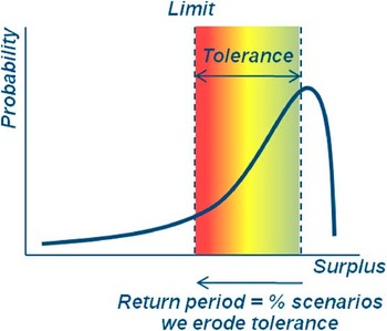
2.19 D'Arcy (Reference D'Arcy2009) argues that risk appetite ‘reflects the multiple dimensions of risk in a very similar way’. Companies have a taste for certain types of risk that others may avoid. This can be due to favourable past experience, specialised expertise or how a risk fits with other aspects of their operations. In ‘Handling uncertainty - the key to truly effective Enterprise Risk Management’ from the Institution of Civil Engineers (ICE) and the Faculty and Institute of Actuaries (2011), ‘risk appetite’ is defined as the amount of risk which is judged to be tolerable. In broad terms a useful risk appetite specifies three items: the floor below which a quantity should not fall; a tolerance which specifies the level of performance which is normally expected; and, a return period which specifies the frequency with which the tolerance is eroded. This is shown illustratively in figure 7. Of course this need not be expressed in purely financial terms.
Specifying risk appetite

Measuring risk appetite
2.20 Ciorciari & Blattner (Reference Ciorciari and Blattner2008) argue that risk appetite must consider the income statement for measuring the effect of a risk on earnings, the balance sheet for determining the impact of risk on key financial ratios, and even off balance sheet items that could affect an organisation's financial position. In these regards, risk appetite should be quantitatively determined as a series of interrelated values or indices.
2.21 In practice, an Economic Capital (EC) approach is adopted by many practitioners in financial organisations as an indicator of risk appetite. Basically, economic capital is an internal measure of the capital needed to survive severe risk scenarios. Conventionally, institutions use this metric to indicate their risk tolerance and hence represent their appetite for risks. However, the capital-centric approach may not incorporate all risks, e.g. reputational risk, and does not always result in an optimal level of risk. In order to overcome such shortcomings, value-based approaches are proposed to enable a truly enterprise-wide definition of risk appetite.
2.22 A value based approach is based on a company's internal capability to mobilise internal resources for ERM. A central element in the value-based approach is to start by examining the organisation's strategy and build a model to calculate an internal valuation of the firm based on achieving the strategic plan. A technique, known as Failure Modes and Effects Analysis, can be employed to identify and quantify the most important risks or their aspects.
2.23 A value based approach can enhance the internal buy-in, and develop a more collaborative approach that leverages existing internal risk management expertise, and identify and quantify some of the most important threats to the firm. In addition, the approach led to an enhanced perception of the company by key external stakeholders.
2.24 D'Arcy (Reference D'Arcy2009) suggests that the analysis of risk appetite should be based on aggregated results of all of the risks, instead of the narrow-viewed economic capital approach. However, due to every organisation's specific characteristics and detailed methods implemented, risk appetite statements from different organisations are not comparative.
Applying risk appetite
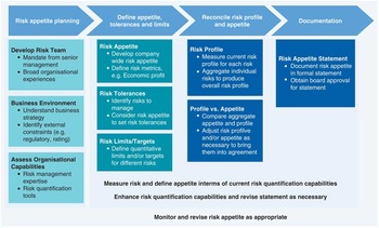
2.25 There are quite a few attempts of implementing risk appetite into the management of insurance companies. For instance, Batty & Dalenta (Reference Batty and Dalenta2010) presented a flowchart, as shown in figure 8, for practitioners to apply risk appetite in operations.
Applying risk appetite, adapted from Batty & Dalenta (Reference Batty and Dalenta2010)

2.26 The model breaks down risk appetite exercises into four phases, namely: risk appetite planning; defining appetite, tolerance, and limits; reconciling risk profile and appetite; and documenting the outputs. All of these are composited by specific activities. As can be seen, this process can perform better if it is implemented in synergy with an organisation's ERM framework.
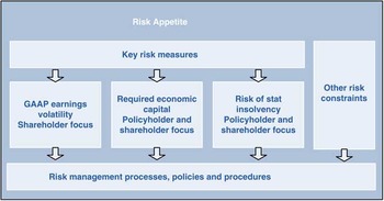
2.27 On the other hand, Korthals & Chase-Jenkins (Reference Korthals and Chase-Jenkins2010) provide an alternative perspective as illustrated in figure 9.
Applying risk appetite, adapted from Korthals & Chase-Jenkins (Reference Korthals and Chase-Jenkins2010)

2.28 In Korthals & Chase-Jenkins’ model risk appetite is more than an internal issue and it should meet investors’ and policyholders’ expectations as well as solvency and regulatory requirements. Guidance of best practice in determining a risk appetite statement is provided by Korthals & Chase-Jenkins as follows:
• There is an implied contract between the Board and management as to how much they are willing to put at risk and for what level of return.
• The risk appetite is articulated explicitly – transparency and communication to stakeholders are critical.
• A common metric is in place to understand key individual risks and how much in total is at risk across the organisation and is used to optimize risk/return within the risk tolerance and risk limits.
• The risk profiles of the business units and the enterprise consider stress events to ensure the company can withstand unexpected events.
• Risk limits for individual business activities are established through a quantitative, bottom-up aggregation process.
• The top down risk tolerances are modelled and reconciled for consistency with the bottom up risk limits.
• Adherence to the risk appetite, risk tolerances and risk limits is monitored and reported.
Risk appetite in a regulatory context
2.29 In recent years, regulators across the world have begun to regard risk appetite as a pivotal aspect of risk management in financial institutions. The Committee of European Insurance and Occupational Pensions Supervisors (CEIOPS, replaced by EIOPA from 1 January 2011), repetitively mentioned risk appetite as the core in risk management and a clear statement of risk appetite is expected in the risk management framework.
2.30 An EC (2010) report highlighted that in the financial services sector:
‘It is important to avoid any moral hazard by not diminishing the responsibility of private stakeholders. It is therefore the responsibility of the board of directors, under the supervision of the shareholders, to set the tone and in particular to define the strategy, risk profile and appetite for risk of the institution it is governing’.
2.31 The “shareholders” referred to above can be more generally thought of as the providers of capital, e.g. members in the mutual sector. The Commission also concludes that their failure to identify, understand and ultimately control the risks to which their financial institutions were exposed is at the heart of the origins of the current financial crisis. Several reasons or factors contributed to this failure: boards of directors were unable or unwilling to ensure that the risk management framework and risk appetite of their financial institutions were appropriate.
2.32 A common theme from regulatory bodies is that ‘few firms can properly articulate their overall risk appetite’ and ‘board-level directors should be involved in determining risk appetite’. In particular, it has been found that appetite for operational risk is even harder to realise as quantitative methods are inapplicable in this area. Furthermore, reports (GAO, 2009; FSA, 2006a) produced by the US and UK regulators’ implied that high-level management does not fully understand the importance of risk appetite and is not actively involved in its determination.
2.33 From a regulator's viewpoint, the significant issues in risk appetite application are:
• Producing meaningful statements of risk appetite has posed significant challenges for many firms.
• Although most firms have defined their risk appetites, there has been slow progress by boards and management to go beyond definition and apply them as a point of reference for material decision making.
• Many firms have not cascaded their appetite statement to operational and technical staff.
• Applying a risk appetite to operational issues has proved challenging for most firms.
• Only a few firms to date, as part of their embedding of the ICASFootnote 3 process, have considered establishing a link between their risk appetites and their management of solvency.
• Some firms have not consistently monitored adherence to their risk appetites or reviewed them for some time.
There appears to be a big step between defining and applying risk appetite.
Risk appetite and management behaviour
2.34 Much of the behavioural theory applied to the understanding of managerial risk taking has been based on the work of Kahneman & Tversky (Reference Kahneman and Tversky1979) on the risk propensity of individuals. Kahneman & Tversky identify that individuals evaluating options tended to try to simplify decision making by the use of heuristicsFootnote 4 and that they were also prone to personal biases. They concluded that even experienced researchers can show bias when they think intuitively in connection with complex problems, often forgetting fundamental statistical rules. In decision theory the subjective probability of a given event occurring is essentially the quantified opinion of an idealised person. The derived probability is subjective in the sense that different individuals will have different probabilities for the same event. While the subjective probability approach should allow a rigorous subjective interpretation of probability, this is not enough in practice as the judgements will be compatible with the beliefs held by the individual decision maker. The rational individual will attempt to make probability judgements compatible with their knowledge of the subject matter, the laws of probability and their own judgemental biases. These factors influence the decision maker's perception of the risk.
2.35 Bromiley (Reference Bromiley1991) and Fiegenbaum & Thomas (Reference Fiegenbaum and Thomas1988) describe an extension of prospect theory to the firm. They argued that a firm's aspirations serve as target or reference levels. Firms anticipating returns below the relevant reference level will be risk seeking while those above will be risk averse. Palmer & Wiseman (Reference Palmer and Wiseman1999) also point out that when decision makers are faced with the prospect of failing to meet their objectives, they accept higher risk options that offer an opportunity to attain the objective and avoid the loss. In contrast, when decision makers think they will achieve their goals they will take the safer options that avoid jeopardising the attainment of the goals.
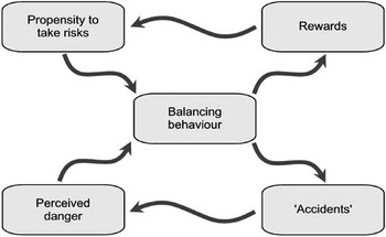
2.36 Adams’ (2001) model of risk compensation is shown in figure 10. The model shows that an individual's risk propensity and perceptions are interdependent and adapt as a result of past outcomes (rewards or accidents).
Risk Compensation Mode (Adapted from Adams, Reference Adams2001)

2.37 Risk compensation theory postulates that when individuals make decisions involving risk they balance the expected rewards of their actions against the perceived costs of failure. In other words they carry out a balancing act in which their perception of the risk is weighed against their propensity to take the risk. This propensity to take risk depends in part on the potential rewards and partly on the decision makers’ risk preferences and prior general appetite for risk.
2.38 Adams (Reference Adams2001) describes the ‘balancing behaviour’ within his risk compensation model as being governed by the individual's risk preference, or his ‘risk thermostat setting’, or ‘comfort level’, or ‘risk appetite’ in this study. As described, Adams postulates that all individuals have a ‘risk thermostat’ that defines a level of risk with which they are content.
2.39 Adams goes on to claim that it also varies ‘from one group to another’ and ‘from one culture to another’ but states later that the risk compensation hypothesis is ‘an explanation of individual, not collective, behaviour’. For this reason he claims that risk is not reduced by the efforts of risk managers but, rather, it is redistributed.
Summary
2.40 As can be seen from the literature, there is no agreed definition of risk appetite as groups hold different viewpoints based on their experience and knowledge. Integrating all the relevant perspectives the authors proposed a working definition of risk appetite as:
“the degree of comfort and preference for accepting a series of interconnected uncertainties about achieving corporate goals.”
2.41 In the same spirit of integration, eight key guidance points for applying the risk appetite concept in an organisation, with particular focus on the insurance sector, are given below:
1. Be systematic and holistic in nature.
2. Be integrated into the organisation's ERM framework.
3. Have high level involvement in an organisation, often board level.
4. Have alignment with an organisation's strategy, policy and culture.
5. Should be consistent over time but can be reviewed, audited and modified regularly.
6. Utilise both quantitative and qualitative measures and methods.
7. Be capable of dealing with new and emerging risks.
8. Should incorporate stakeholder, regulator and or policy holder's expectations.
3. Overview of emerging risks
3.1 According to a report presented by the International Actuarial Association (2008, page 37), emerging risks are ‘developing or already known risks which are subject to uncertainty and ambiguity and are therefore difficult to quantify using traditional risk assessment techniques’. For the purposes of this paper we use the term emerging risk to include the categories of risks, ‘hard to define risks’ and ‘systemic risks’, although a brief description of each is given in the following sections for completeness.
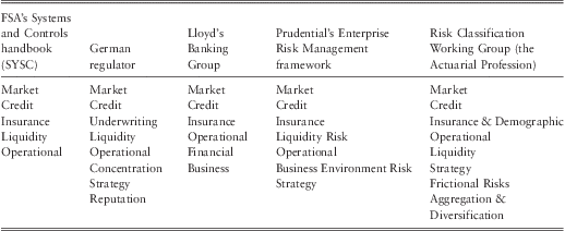
3.2 The reason why emerging risks are problematic is because, by their very nature, they are not well addressed and tend to come as a surprise. In practice, a wide range of risk classification methods are used in an attempt to cover the existence of most risks, thereby reducing the surprise. Unfortunately, any classification cannot be complete as new risks emerge making the functionality of the classification system subject to the time point of observation. Moreover, most risk classification methods adopt a reductionist approach to break risks down into components, which then use those elements to categorise risks.
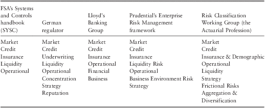
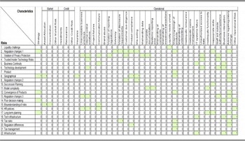
3.3 Kelliher et al. (Reference Kelliher, Wilmot, Vij and Klumpes2011) have conducted research on risk classification frameworks and present a very useful classification set, presented in summary form here in table 1. The full list is extensive at over 250 categories, which, if combined with the concept of risks having multiple characteristics, could be extremely useful in identifying emerging risks. These sorts of classification and risk characteristic systems are becoming increasingly powerful when linked with enterprise wide software database systems.
Risk classification review (Adapted from Kelliher, Reference Kelliher, Wilmot, Vij and Klumpes2011)
Features of emerging risks
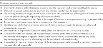
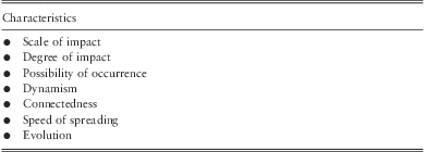
3.4 Although the concept of emerging risk is still developing it is possible to summarise the research on the key features of emerging risks shown in table 2.
Key features of emerging risks

Emerging Black Swans
3.5 Nassim Taleb (Reference Taleb2007), in his book ‘The Black Swan’, articulates the theory of the black swan. In general, the theory is composed of three pillars:
1. Rare events, especially those never seen before, have disproportionate levels of impact and are beyond people's conventional comprehension;
2. Identifying those rare events is beyond the capability of conventional methods, especially numerical methods;
3. Those rare events are a challenge to people's worldview. It is also pointed out that psychological biases, either individually or collectively, prohibit understanding uncertainty, as people always use historical data to judge the future and neglect the roles of rare events in the course of history.
3.6 In order to define a black swan event, Taleb describes three attributes. First, a black swan event has extraordinary impacts. Second, it is an outlier and is outside of the realm of regular expectation. Historical probability cannot convincingly predict the event. Third, people can only explain the event after its occurrence, making interpretation a posterior activity. Collectively this means that limited prior knowledge is available in relation to a black swan event. Examples of black swan events in recent decades could be: the development of personal computers and the internet; terrorist attacks; the collapse of a country; and, a global financial market turmoil caused by subprime crisis. Following such logic, Bayesian statistics can be applied to test people's knowledge regarding a real world scenario and then Bayesian inference can be used to update information as evidence emerges.
3.7 It should be noted that, the term ‘black swan’ used by Taleb originates from the work of the German philosopher Popper who questioned the value of traditional scientific positivism methodologies and instead proposed an approach of falsification and exception as the way to push discovery and theory forward.
Emerging risks and black swans
3.8 Fundamentally, the existence of a black swan is due to our blindness when dealing with uncertainty. Current approaches look back into historical data to draw patterns and use such patterns to predict the future. This mechanism is like driving a car on a bumpy country road with nothing but a rear-vision mirror: one only knows what has passed and what the surface of the road was like. This sort of information is useful for providing a general impression of the road and to make predictions on how the road might look ahead, however it cannot predict the next turn or an obstacle ten meters away.
Looking beyond black swans
3.9 Although the black swan theory articulates that the utility of prior information is significantly constrained when predicting black swan events, near future events can be decoded. The time difference between a future event and the observation time point determines whether the event is a black swan event or not. For instance, the emergence of internet technology is a black swan phenomenon for people living in the 1960s. However, it was not a total surprise in the mid-1990s as computer technology, especially personal computers, was advanced enough to provide the infrastructure and people never stopped their pursuit for better communication. Or in other words, the mid to long term future are full of black swan events, but there may be some clues for the near future, implying that the observation point is in fact another determinant for black swan events.
3.10 Using biology to look at the black swan problem makes emerging risks appear somewhat more predictable. We have seen white swans all the time and black birds are common everywhere. So, at least in evolutionary terms, a black swan is a strong possibility. It is certainly more likely than a 3-winged, green and purple striped swan. In these regards, we believe that, given an appropriate time point, the prior signal of an event can be observed using biological evolutionary system methods. If the newly emerged DNA can help the offspring survive the environment better, it is likely to be passed to its descendants. Otherwise the emergence will stop at the offspring level. Over a period of time, the accumulations of newly developed features make the offspring a standalone species and such a process produces ‘black swans’ in the biological world. Evolutionary approaches are perhaps a more natural and intuitive direction to look for emerging risk understanding, as postulated by Allan et al. (Reference Allan, Yin and Cantle2010). Such an approach is currently applied, in the pharmaceutical industry to predict the evolution of viruses and then develop antibiotics in advance.
Linking systemic risks and emerging risks
3.11 This study primarily focuses on emerging risks but there are a number of similarities with systemic risks, both in their description and behaviour, which warrant a short discussion. Some common features and attributes shared between systemic and emerging risks are:
• They are both highly linked to interactions.
• They can use the same management process, as stated by Ingram (Reference Ingram2010).
• They can expose the organisation to a similar degree of impacts.
• They can lead to huge losses among interconnected institutions.
• They can be triggered by similar events.
• They are interchangeable in many circumstances.
• They can affect the organisation's strategic objectives.
Some useful definitions of systemic risk are provided below.
Systemic risks as emerging risks
3.12 In relation to the recent financial crisis, Besar et al. (Reference Besar, Booth, Chan, Milne and Pickles2011), reviewed a number of definitions of systemic risk, and proposed a new definition:
‘A systemic risk materialises when an initial disturbance is transmitted through the networks of interconnections that link firms, households and financial institutions with each other; leading, as a result, to either the breakdown or degradation of these networks.’
Such a definition highlights the interconnected nature of participants in the financial market and it is the network of participants that realise the possibility of a systemic risk.
3.13 Helbing (Reference Helbing2010) defines systemic risks as ‘the risks that can trigger unexpected large-scale changes of a system or imply uncontrollable large-scale threats to it,’ emphasising the fact that effects of systemic risks are disproportional to the size of the initial risks or shock.
3.14 COSO (2004) explains why systemic risk is harder to manage than conventional risks.
‘Systemic risk, unlike conventional risks whose negative impacts can be assessed and managed, emanates from either internal or external sources and occurs so promptly that it leaves little time for management to respond. Such a risk not only affects an institution's ability to achieve objectives, but also influences other institutions via connections.’
3.15 The Counterparty Risk Management Policy Group (2008), a collection of senior decision makers in leading financial institutions, made five recommendations for controlling systemic risks, regardless of the degree of the understanding in systemic and emerging risks. Table 3 provides a brief summary of their recommendations.
Five recommendations (CRMPG III, 2008)

3.16 A recommendation of particular interest is that the systemic risk exposure of an institution is related to its risk appetite. Moreover, appropriately estimating risk appetite can reduce the possibility of being affected by a systemic risk.
Conclusion
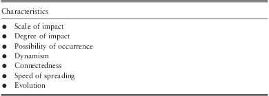
3.17 In order to achieve a comprehensive understanding of the emerging risks concept, it has been rationalised that ‘hard to define risks’ are equivalent to emerging risks which in turn have considerable similarities with systemic risks. The key features of emerging risks are summarised in table 4 from different sources of literature.
Characteristics of key features of emerging risks
3.18 The black swan theory is reviewed in the context of emerging risk. It is argued that, in the near future, black swan risks may give out some clues that can be identified and modelled. The practical application of this thinking will be explained in Chapter 5.
3.19 Emerging risks are difficult to identify because of the combination of their dynamic, highly interconnected and evolutionary nature. In other words they behave like the outputs from a complex adaptive system.
4. An overview of systems science
“The more we study the major problems of our time, the more we come to realize that they cannot be understood in isolation. They are systemic problems, which mean that they are interconnected and interdependent.” (Capra, Reference Capra1996)
Introduction to systems thinking, complexity and complex systems
4.1 Systems thinking is both a worldview that:
• Problems cannot be addressed by reduction of the system;
• System behaviour is about interactions and relationships; and,
• Emergent behaviour is a result of those interactions.
And a process or methodology:
• To understand complex system behaviour;
• To see both the “forest and the trees”;
• That can identify possible solutions and system learning; and,
• That utilises complexity science and other disciplines.
4.2 The development of complexity science is a shift in scientific approach towards an interdisciplinary paradigm with the potential to profoundly affect business, organisations and government. The goal of complexity science is to understand complex systems: what rules govern their behaviour, how they manage change, learn efficiently and optimise their own behaviour.
Systems thinking
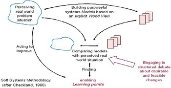
4.3 The origins of systems thinking can be traced back at least 2,500 years to the ancient Greek philosophers. It is different from, but complementary to, other ways of thinking, such as scientific reductionism, for example. This postmodern thinking led to difficulties managing the fit between engineering and physical science's quest for determinism through a reductionist paradigm and ideas of emergence, paradox, disorder and self-organisation (Jackson, Reference Jackson2004). Checkland (Reference Checkland1999), a computer scientist by training, introduced a distinction between hard systems and soft systems as a bridge:
• Hard systems of the world are characterised by the ability to define purpose, goals, and missions that can be addressed via engineering methodologies in attempting to, in some sense, ‘optimise’ a solution.
• Soft systems of the world are characterised by extremely complex, problematical, and often mysterious phenomena for which concrete goals cannot be established and which require learning in order to make improvement. Such systems are not limited to the social and political areas and also exist within and amongst enterprises where complex, often ill-defined patterns of behaviour are observed that are limiting the enterprise's ability to improve.
4.4 Systems thinking is essentially the process of discovery and inquiry that uses techniques to understand the interrelationships and underlying patterns of problems and opportunities. Systems thinking is used to address complex problems and can be applied in any discipline or practice.
“Systems thinking enables you to grasp and manage situations of complexity and uncertainty in which there are no simple answers. It's a way of ‘learning your way towards effective action’ by looking at connected wholes rather than separate parts. It's sometimes called practical holism.” (Open University, 2011)
4.5 Peter Senge (Reference Senge1990) in his seminal work on learning organisations describes systems thinking as:
• A discipline for seeing wholes
• A framework for seeing interrelationships, for seeing patterns of change rather than static snapshots
• A set of general principles distilled over the course of the twentieth century, spanning fields as diverse as physical and social sciences, engineering and management
• A specific set of tools and techniques.
4.6 The definition of systems thinking has evolved over time as advances have been made in systems theory. Some additional examples of systems thinking definitions are as follows:
• What is often called systemic thinking is a bundle of capabilities, and at the heart of it is the ability to apply our normal thought processes, our common sense, to the circumstances of a given situation. (Dorner, Reference Dorner1996).
• Systems thinking requires a consciousness of the fact that we deal with models of our reality and not with the reality itself. (Ossimitz, Reference Ossimitz1997).
• Systems thinking provides a powerful way of taking account of causal connections that are distant in time and space. (Stacey, Reference Stacey2000).
• Kasser (Reference Kasser2011) defines systems thinking from a broader perspective of holism: ‘holistic thinking is defined as the combination of analysis (in the form of elaboration), systems thinking and critical thinking’.
• Blockley & Godfrey (Reference Blockley and Godfrey2000) use three key ideas as a framework for describing systems thinking ideas, shown diagrammatically and explained in Appendix B.
• Finally, Blockley (Reference Blockley2005) provides perhaps the most pertinent definition for the purposes of this study: ‘The role of systems thinking is to integrate the language of uncertainty and complexity and its expression in risk, as well as managing risk in terms of two systems the ‘hard’ embedded in the ‘soft’.’
Complex Adaptive Systems (CAS)
4.7 In essence a complex system, or complex adaptive system (CAS), is ‘an explanatory framework for helping people to understand complexity’ (Stacey, Reference Stacey2000). A CAS consists of many agents that interact with each other at multiple interfaces and across layers. The weather system is an example with air, water and heat interacting across interfaces and layers such as clouds or the sea. With time, dynamic patterns of system behaviour emerge from these local interactions between system elements and can even change the structure and nature of the local elements. CAS are also found in social settings, including organisations, and are sometimes referred to as ‘human activity systems’. CAS change their behaviour to adapt to changes in their environment – which is exactly the sort of problem thrown up by enterprise risk management. To make the situation even more interesting, people are also complex adaptive systems, and therefore the agents in the enterprise risk system are themselves CAS.
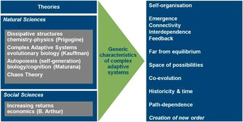
4.8 Mitleton-Kelly (Reference Mitleton-Kelly2003) has outlined the generic properties of a CAS as shown in figure 11.
Complex adaptive system characteristics (Mitleton-Kelly, Reference Mitleton-Kelly2003)

4.9 To some extent, the connectivity, interdependence and feedback properties of a CAS are due to the physical and logical structure of the system. Under such a structure, elements interact with each other, giving rise to unpredictability, intentionality, emergence, evolutionary change and complexity. Complex patterns can arise from the interaction of agents that follow relatively simple rules. These patterns are “emergent” in the sense that new properties appear at each level in a hierarchy (Holland, Reference Holland1995). For example, the structure of a snowflake or a broccoli follows simple rules, closely related to fractals. CAS however can also exhibit ‘self-organising’ behaviour: starting in a random state, they usually evolve toward order instead of disorder (Kauffman, Reference Kauffman1993). The behaviour of a CAS is nonlinear and can be sensitive to small differences in initial conditions, so that two systems with very similar initial states can follow radically divergent paths over time. Consequently, historical accidents may “tip” outcomes strongly in a particular direction (Arthur, Reference Arthur1990). Furthermore this occurs in a similar fashion to the evolution process described by Charles Darwin in his Theory of Evolution (Nelson & Robinson, Reference Nelson and Robinson1982), granting path-dependency and evolutionary properties to the CAS.
4.10 CAS resist simple reductionist analyses, because interconnections and feedback loops preclude holding some subsystems constant in order to study others in isolation. Because descriptions at multiple scales are necessary to identify how emergent properties are produced (Bar-Yam, Reference Bar-Yam1997), reductionism and holism are complementary strategies in analysing such systems (Fontana & Ballati, Reference Fontana and Ballati1999). It is an inclusive approach that does not attempt to dismiss, but indeed complements, scientific approaches.
4.11 Not surprisingly, a key property of CAS is complexity itself. Complexity science developed later than systems science yet their mutual development is itself complex, interwoven, adaptive and important as demonstrated by figure 12.
Roadmap of the development of complexity science (Wikipedia, 2010)

Complex Adaptive System Lifecycles
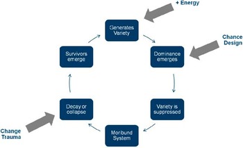
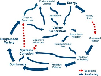
4.12 Hitchins (Reference Hitchins2007) describes how interconnected systems driven by an external source will tend to a cycle of progression in which system variety is generated; dominance emerges and suppresses the variety; the dominant mode decays or collapses; and survivors emerge to regenerate variety. Romme & Despain (Reference Romme and Despain1989) demonstrate this in natural systems with a classic example of why major forest fires are relatively rare (1:40 years) in Yellowstone National Park, despite the fact that lightening fires occur almost every year.
4.13 The process and the concept is expanded and described in detail in Appendix A and Hitchins (Reference Hitchins2007) argues that the same process occurs in financial markets, organisations, societies or, indeed, any open complex system with an energy or information source. The significance of this lifecycle model is that it provides an insight into how systems evolve and change over time and, most interestingly, what the likely causes of the downfall are and what might be done to prevent it.
Complex Adaptive Systems and Insurance Companies
4.14 An important aspect of social and economic systems is that they are complex systems and (re)insurance companies make no exception. The Geneva Association (2010), a leading think tank in the industry sector, perceives insurance companies as complex because an insurance company:
• Operates diverse types of activities through numerous legal entities (e.g., simultaneously operating banking, insurance and fund management subsidiaries);
• Operates across borders with centrally managed capital and liquidity (as opposed to simpler networks of national subsidiaries); and,
• Has exposures to new and complex products and markets that have not been sufficiently tested.
4.15 The commonality of complex systems can be traced in insurance companies, i.e. a large number of interacting (mutually coupled) system elements (such as individuals, companies, countries, cars, etc.). These interactions are usually dynamic and nonlinear. Typically, such systems tend to be dynamic rather than static, and probabilistic rather than deterministic, exactly the same as an insurance company. The lack of predictability and controllability can be partly attributed to externality, i.e. exogenous events, and partly to the internal mechanism of the system.
4.16 A report by the American Society of Actuaries (Mills, Reference Mills2010), entitled, Complexity Science: An introduction (and invitation) for actuaries, emphasises the need for a new breed of actuaries who understand the complex nature of social systems. We highly commend this report to readers. A brief set of conclusions can be found at the end of Appendix A.
Complexity science
4.17 A significant amount of work has been done under the umbrella of complexity without a universal agreement upon its precise definition. As traced by Gell-Mann (Reference Gell-Mann1995), the English word ‘complex’ is derived from the Latin word ‘complexus’, which means braided or entwined together. Mitleton-Kelly (Reference Mitleton-Kelly2003) termed complexity as the inter-relationship, inter-action and inter-connectivity of elements within a system and between the system and its environment. A good example of a complex system is the financial market, in which a large number of investors, brokers, agencies, regulators, and other participants are interconnected and interact with each other.
4.18 Paradoxically, some complex interactions among highly differentiated parts can produce surprisingly simple, predictable behaviour, featuring simple laws and rules (Anderson, Reference Anderson1999). Cohen & Stewart (Reference Cohen and Stewart1994) summarised this nicely by pointing out that normal science shows how complex effects can be understood from simple laws; chaos theory demonstrates that simple laws can have complicated, unpredictable consequences; and complexity theory describes how complex causes can produce simple effects.
4.19 Kauffman (Reference Kauffman1993), on the other hand, takes a slightly different perspective, seeing complexity as the principal related to non-linear properties of a system. This non-linearity is often associated with the uncertainty of complex situations. Uncertainty, so central to modern risk management, has a special relationship with complexity as more complexity increases uncertainty and increasing uncertainty can be a key influence in increasing complexity.
4.20 With respect to social systems, Daft (Reference Daft1992) equates the level of complexity with the number of activities or subsystems within the overall system, noting that it can be measured along three dimensions. Vertical complexity is the number of hierarchical levels, horizontal complexity is the number of elements across the whole system, and spatial complexity is the number of geographical locations. Time is often considered a fourth dimension of complexity, in that a system can interact with its environment and thus evolve over time.
Summary and relevance to Risk Appetite and Emerging Risk
4.21 This section details why and how complex system approaches and techniques are particularly useful in the context of this research.
Risk Appetite
4.22 Risk appetite is not a single stand-alone concept; many interdependent and connected components form a risk appetite, e.g. we are unlikely to have an aggressive appetite for longevity risk if we have limited capital and extensive legacy risk. The real world relationships between different components give rise to feedback mechanisms, presenting potentially nonlinear behaviour of the system. For instance, an equity shock which weakens a firm and leads to regulatory intervention, in turn leading to a loss of confidence with downgrades, persistency problems and a collapse in new business.
4.23 Further, the effects brought by those interacting relationships become less predictable over time and this is referred to as emergence.
4.24 Further, risk appetite, in practice, is often expressed as a statement that includes multiple inputs, not all of which can be explicitly represented by a single value. In that, probability states or fuzzy sets are more appropriate for describing the nature of risk appetite. Over time, a company can change its risk appetite because the business and regulatory environment are dynamic resulting in changes to risk capacity (how much risk a company can take as constrained by its available resources). This property is characterised as evolution or co-evolution. During the course of evolution, a company may encounter different scenarios and these events can gradually re-shape the risk appetite and risk capacity. Over time, risk appetite is dependent upon the path of the decision-making exercises and external environment of the company.
Emerging Risk
4.25 Emerging risks are the emergence of unintended consequences as a result of complex interactions between strategic objectives, existing risks, risk management interventions, business and regulatory environment, markets and people's behaviour. Historically, emerging risks are dependent upon these interactions and this is referred to as path-dependence.
4.26 An important source of emerging risk is the combination and integration of existing risks, or subsets of their characteristics. For instance, when people input incorrect data into a newly established IT system, this operational risk may cause serious problems in other fields, such as financial reporting or reputational risks through poor servicing. The combined symptom can be understood as an emerging risk but in fact it is deeply rooted in existing risks – it is the combination and integration of existing risks that often give rise to new risks.
4.27 As noted, risks within a company or an organisation are highly interdependent and connected both to each other and to the environment they exist and evolve in. When they are away from an equilibrium state, mitigation actions do not function properly, and may cause additional effects that propagate through a network of risks. For example, market volatility brings down equity prices and reduces the underlying value of a company's assets. If the reduction is significant, rating agencies may decide to downgrade the company's rating, making it more difficult or expensive to raise funds. The deterioration in their financial situation forces the company into a spiralling loop that feeds information back into the system.
4.28 Emerging risks do not suddenly appear from nowhere and there are always possible leading indicators, even though they may be hard to recognise. Emerging risks are the product of an evolutionary process and it takes time for them to be realised.
4.29 Complex systems concepts appear to closely relate to the problems of defining risk appetite and identifying emerging risks. This allows us to bring a wide range of tools and techniques from systems and complexity science to bear on our problem. The next section discusses some possible prominent methodologies and their application.
5. Complexity science and complex systems tools & techniques
5.1 As discussed in Chapter 4, a systems thinking paradigm helps solve the challenges of describing risk appetite and enables appropriate risk limits to be attached to key business drivers; and makes identifying emerging risks from their underlying drivers philosophically viable. Furthermore, systems and complexity science provide a rich pool of possible tools and techniques that may be useful for this specific study. The next task is to select the most appropriate technique(s), from the broad spectrum available, to address these two problems, individually or collectively.
Requirement Specifications for the Tools & Techniques
5.2 By summarising the specific nature and characteristics of the ‘risk appetite’ and ‘emerging risk’ problem, it was determined that a candidate solution or methodology must satisfy the following eight criteria to some extent:
Soft systems criteria
1. Rigour: the solution shall be based on rigorous quantitative methods;
2. Expert interaction: expert knowledge shall be integrated into the solution;
3. Adaptation: the ever changing nature of the problem shall be properly reflected;
4. Computability: it takes a reasonable time to arrive at results.
Hard systems criteria
1. Data requirement: the solution shall be viable regardless of the availability of hard data;
2. Accuracy of results: precision is preferable;
3. Operability: non-academic business users can repeat the method for their own purposes;
4. Application availability: the methodology shall be based on software packages that are affordable by a wide range of organisations but scalable to multi-national group solutions.
5.3 The eight criteria do not exist in isolation and they are in fact intertwined. Nonetheless, they have been used as individual measures in order to select the most appropriate tools using a Likert Scale type measurement to quantify each as shown in table 5.
Measurement of Criteria

Visualising the options
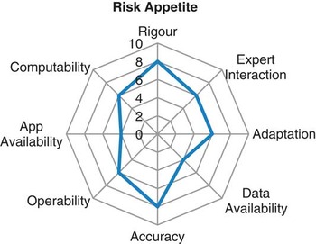
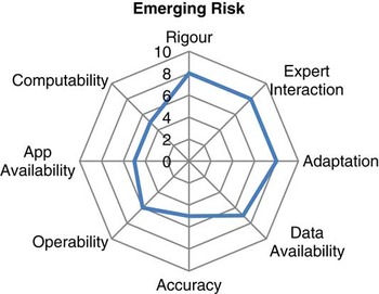
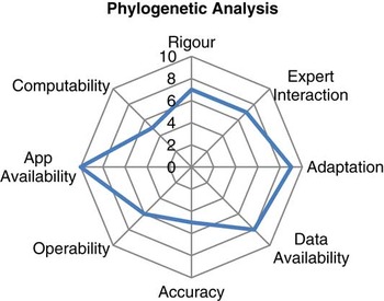
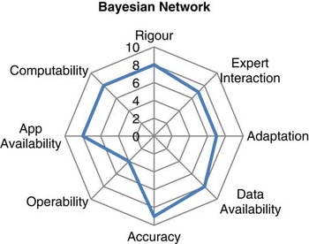
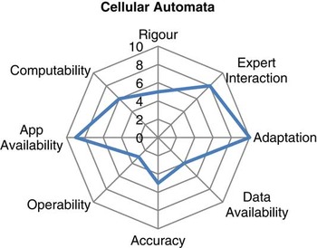
5.4 With the above measurement regime, the two problems can be specified against the criteria to portray the ideal tool, displayed as radar diagrams in figures 13 & 14.
Radar map showing benchmark for evaluating tools for the Risk Appetite problem

Radar map showing benchmark for evaluating tools for the Emerging Risk problem

5.5 The radar maps illustrate the requirements for the proposed methodologies visually. Theoretically, the radar map of a perfect methodology to tackle a problem should exactly fit the corresponding radar map of the problem. However, due to the usual practical constraints, no perfect match is expected and therefore the task for selecting a methodology in the systems and complexity science domains is to find the ‘best match’.
A rationale of the Systems and Complexity Science Tools Reviewed
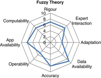
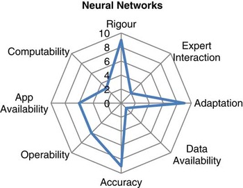
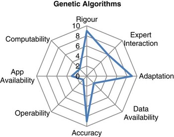
5.6 This research has reviewed eleven of the most prominent systems and complexity science approaches: Concept Mapping, Systems Dynamics Modelling, Chaos Theory, Fuzzy Logic Theory, Neural Networks, Genetic Algorithms, Phylogenetic Analysis, Bayesian Belief Networks, Cellular Automata, Agent Based Modelling, and Network Theory. Each is briefly described in the following sections and assessed against the measurement regime in table 5.
Concept Mapping
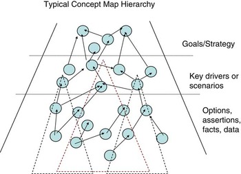
5.7 Concept mapping is a technique to visualise the complex and nonlinear relationships between different concepts. According to studies conducted by Novak (Reference Novak1998), existing knowledge facilitates one's assimilation of new knowledge and so the ability to utilise, and hence exploit, existing understanding becomes pivotal. Abstract or concrete concepts can be denoted as nodes and their interrelationships can be visualised as links so that they formulate a system in the appearance of a map.
5.8 This allows the use of analytical techniques to identify potent concepts or patterns. In doing concept mapping exercises, one can capture an explicit view of existing knowledge and learn from it. However, concept mapping is often perceived as a qualitative technique because of its inability to produce hard numerical results.
The radar map for Concept Mapping is illustrated in figure 15.
Radar map for concept mapping

Systems Dynamics Modelling
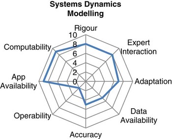
5.9 Systems dynamic (SD) modelling can help users understand the nonlinear relationships of different elements and allows users to include their subjective judgements in models. Once a model is established, the system can simulate future scenarios using deterministic rules as well as random values. A significant advantage of this method is to understand the internal structure of a system, such as feedback or feed-forward loops, and how properties emerge from the interacting elements. A noticeable drawback of such a technique lies in its validation and verification. It is not usually the case that all assumptions can be rigorously tested. In practice, the explanatory functionality of SD modelling is more valuable than its capability in making accurate numerical predictions. The radar map for SD is illustrated in figure 16.
Radar map for SD modelling

Chaos Theory
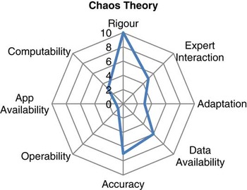
5.10 Chaos theory is extensively employed to explain complexity, dynamics, and the nonlinearity of a system. A small change to the input or the initial state of a system, which is usually expressed in mathematical equations, can lead to disproportionate consequences. This phenomenon is often referred to colloquially as ‘the butterfly effect’. In fact, chaos theory effectively elucidates how a system adapts to both internal changes and external shocks. The application of chaos theory is largely subject to the generalisation of mathematical equations of a system, and this can present significant practical challenges in real life situations. However, attempting to apply chaos theory is an effective organisational learning process to understand the system better. Not many software vendors compete in this market area so, even if a solution was produced as part of this research, users will probably need significant programming knowledge before tailoring any tool for their own analysis.
The radar map for Chaos Theory is illustrated in figure 17.
Radar map for chaos theory

Fuzzy Theory
5.11 Uncertainty and vagueness in information limit the functionality of traditional methods that are based on crisp logic. Fuzzy theory is developed to overcome this insufficiency by taking account of ambiguity in information. A number can be crisp as well as fuzzy, which recognises the ‘degree of truth’. In doing so, set theory, which is the foundation of probability theories, is converted into fuzzy set theory and all subsequent applications are updated to be able to incorporate fuzziness. When using fuzzy logic, people's qualitative description as well as quantitative estimation can be elaborated to maximise its utility. Regarding the applicability aspect of fuzzy theory, the major concern is the efficiency of converting uncertainty and vagueness into fuzzy values. The concepts of fuzzy logic have been widely applied in engineering and artificial intelligence but general practitioners still find the concepts a little difficult to engage with. The radar map for Fuzzy Theory is illustrated in figure 18.
Radar map for fuzzy theory

Neural Networks
5.12 A Neural Network, or an Artificial Neural Network (ANN) in particular, is an automated multi nonlinear regression process. The structure and mechanism of ANN is inspired by human neurons and ANN can equip certain learning capability. With such a capability, ANN can be applied to make predictions and recognise patterns as well as other purposes. Although there are a number of ANN software packages available on the market, most of them appear to be like a “black box” to users and require a degree of skill in parameterisation. If one wants to operate a fully customised ANN, i.e. specially designed artificial neurons or neuron hierarchies, it would be necessary to have extensive programming as well as mathematical knowledge. Some financial institutions already use such models to predict or model risks, but this is a specialist area.
The radar map for Neural Networks is illustrated in figure 19.
Radar map for neural networks

Genetic Algorithms
5.13 The concept of evolution has profound implications in various areas and genetic algorithms (GA) are influenced by this. In most cases, a GA is applied for optimisation purposes. Once the parameters of a problem are decided and a GA model is populated with them, the GA modelling will simulate natural selection processes, i.e. reproduction, mutation, fitness tests and etc. Offspring that carry superior features can survive and their ‘genes’ are passed into the future generation. After multiple iterations, the criteria of a GA might be met or the cost of such a process might be too high to tolerate. The final outputs could be the optimised results. Genetic programming (GP), on the other hand, adopts a similar approach but optimises functions instead of optimising parameters of functions. Up to now, the application of GA is largely constrained by its high requirement on programming knowledge. The radar map for Genetic Algorithms is illustrated in figure 20.
Radar map for genetic algorithms

Phylogenetic Analysis
5.14 Phylogenetic analysis looks into the evolutionary relationships using rigorous mathematical methods. It should be noted that such an evolutionary relationship is not limited to biological creatures but is applicable to any entity that has complex adaptive behaviours. By applying phylogenetic analysis evolutionary relationships of entities can be inferred from which people can obtain classifications of entities, predict emerging entities and hypothesise the properties of those emerging entities. Whilst relatively easy to understand in concept, the algorithmic computational process of phylogeny is relatively complicated but a collection of software is available for this purpose. Perhaps the difficulty in applying phylogenetic analysis lies in its philosophical aspects. The radar map for Phylogenetic Analysis is illustrated in figure 21.
Radar map for phylogenetic analysis

Bayesian Networks
5.15 Bayesian networks (BN), also known as belief networks, are one of the blooming scientific frontiers. Algorithms in BN enable a system to perform inference and learning. Visually, a BN is in a hierarchy structure with nodes cascading in layers, allowing users to visually understand the logic relationships among variables. Software packages are widely available and can deal with the complicated computation processes. They usually provide a range of analytical tools to help carry out a variety of related tasks, such as sensitivity and scenario testing. The radar map for Bayesian Networks is illustrated in figure 22.
Radar map for Bayesian networks

Cellular Automata
5.16 As a particular kind of simulation technique, cellular automata (CA) are very effective in exploring the discrete behaviour of interacting elements in a complex system. The microscopic behaviours of an element, or a cell, can be modelled using simple rules. By interacting with other elements, emergent patterns can be observed. Or in other words, CA enables the aggregated patterns to be understood with a bottom-up approach, which is different from the conventional reductionist paradigm. Thus, CA is a means of facilitating the motif ‘the whole is greater than the sum of parts’. On the other hand, modelling CA requires considerable programming knowledge and behaviour rules must be modified repetitively if accurate results are expected. The radar map for Cellular Automata is illustrated in figure 23.
Radar map for cellular automata

Agent Based Modelling
5.17 Agent based modelling (ABM) is well known for its ability in simulating the behaviours of agents. Each agent is controlled by a set of behaviour rules or decision rules and it can make autonomous decisions or reactions. That is, when the environment changes, an agent makes its own decision to either adapt itself accordingly or do nothing. Such a mechanism allows for the observation of emerging patterns of a system in a prompt manner. Further, ABM provides a direct way to view the nonlinear relationships between agents in a system. Theoretically, most objective-oriented programming environments can facilitate ABM, and there are specific software environments available for ABM from a variety of sources. Whilst ABM is a very powerful modelling technique it has to be used with care if precise values are required and is often best used to explore system behaviours rather than specific values. The radar map for Agent Based Modelling is illustrated in figure 24.
Radar map for ABM

Network Theory
5.18 To some extent, everything is somehow connected and network theory holds this proposition to study relationships. In order to apply network theory, an object is conceptualised as a node (or vertex) and its relationships with others are denoted as edges. Different mathematical theorems, algorithms, and measures can be applied to arrive at useful information such as: clustering and grouping; the identification of cycles; and, the importance of individual nodes to flows around the network. There are many software packages available which can assist with the analysis of networks, but the challenge for most users will be the efficient creation of the network in the first place. The radar map for Network Theory is illustrated in figure 25.
Radar map for network theory

Summary and Final Selection of the Tools
5.19 Their radar maps are shown so that both positive and negative aspects of a tool can be compared to the problem specifications. The data availability issue is a key concern for the Neural Network and Genetic Algorithm tools as these two depend heavily on having a large quantity of time series data, which is not very likely in this research. Furthermore, the operability issue limits the viability of Systems Dynamics modelling, Chaos Theory, Genetic Algorithm, Cellular Automata, and Agent Based Modelling. In fact, these five tools require considerable programming and mathematical knowledge from users. Considering the time and resource limits of most actuaries, these five tools are not likely to be applied on a large scale unless some specifically designed modules are available. Similarly, application availability issues make Chaos Theory and Genetic Algorithms impractical for this study as few ready-to-use software packages are available on market at a reasonable cost.
5.20 Network theory, on the other hand, survives the hard criteria selection but can show little adaptive behaviour of a system. The discrepancy between its existing capability and the requirements of the two problems is so big that it has to be left out.
5.21 Therefore, Bayesian Networks, Fuzzy Theory, Concept Mapping and Phylogenetic Analysis are the remaining candidates for both problems. The former two seem to be able to meet most criteria set by both problems and they are most suitable for the Risk Appetite problem, whilst the Phylogenetic Analysis cannot meet the accuracy requirement of the Risk Appetite problem, yet could be applied to the Emerging Risk problem. It should be noted that concept mapping as a stand-alone technique does not really meet the accuracy test but its capability for robustly eliciting and analysing scenarios could be utilised as an auxiliary tool for both the research challenges. Therefore, the proposed methodology for addressing the two problems will be constructed using Bayesian Networks, Fuzzy Theory, Concept Mapping, and Phylogenetic Analysis whilst keeping other techniques and tools in the background for use if necessary.
5.22 The following chapters will demonstrate how we address real world risk appetite and emerging risk problems using our proposed methodologies.
6. Risk appetite case study – concept mapping and Bayesian networks
6.1 A well-known insurance company was used as a basis for trialling the integrated use of a concept mapping and Bayesian networks (BN) approach. The theory behind concept maps and Bayesian belief networks is briefly explained here and we will take the reader through the various stages of the application to give sufficient detail to allow an experienced practitioner to apply these techniques in their organisations.
Concept Mapping
6.2 A concept map is a model which allows complex interconnected factors to be shown in a simplified diagrammatic form, so that the overall picture can be understood and communicated to a wide audience. Such maps are particularly useful for identifying and analysing strategic issues, as these are often complex in nature and contain a wide range of factors interacting in a nonlinear manner. Also they can help visualise the complex and nonlinear relationships between different concepts.
6.3 The approach is built upon Personal Construct Theory (Kelly, 1991) and Concept Mapping (Eden, Reference Eden1988), which is a soft systems analysis technique. Personal construct theory suggests that we make sense of the world in order to predict how, all things being equal, the world will be in the future, and to decide how we might act or intervene in order to achieve what we prefer within that world (Ackerman & Ackerman, 2004). Cognitive mapping allows an account of a problem to be broken into its constituent elements. These are treated as distinct concepts which are then reconnected to represent the account in a graphical format.
6.4 In the context of risk appetite people have a mental map of the risk exposure they are interested in but their individual view will likely be incomplete, or maybe just hard to make sense of or articulate. Concept maps draw everyone's contribution to the “risk story” which can be used to make a “theory” about the risk appetite and exposure. Abstract or concrete concepts can be denoted as nodes and their interrelationships can be visualised as links so that they formulate a system in the appearance of a map, allowing for analytical techniques to identify potent concepts, structure and key connections. In doing concept mapping exercises, one can capture an explicit view of existing knowledge and learn from it. The technique is particularly helpful for identifying areas where the descriptions from different participants conflict or where parts of the description are too brief and underdeveloped or indeed where they simply don't seem to make sense.
6.5 A simplified concept map that has been reduced in complexity to expose key levers is shown in figure 26. The nodes with lots of interconnections are likely to be worth looking at first. The red nodes (ringed by dotted lines) in figure 27 represent key nodes which are most central in the system and are key levers for action or mitigation; the yellow rectangular nodes are stated goals or aims; and the orange oval nodes are beliefs about the strategic risk and risk appetite. Typically an hour long interview would generate over 100 nodes and need to be analysed by computer programs to identify the key nodes, clusters, loops and hierarchies. In this paper we use a program called, ‘Decision Explorer’,Footnote 5 but other software is available.
Typical concept map hierarchy (after Eden & Ackerman, Reference Eden and Ackerman2004)

An example of a simplified concept map

Bayesian Belief Networks
6.6 Bayesian Networks (BNs), also known as belief networks or Bayesian Nets for short, are a directed acyclic graph (DAG) model to represent knowledge about uncertain domains. A DAG model is composed of a set of nodes (vertices) and directed edges. In that, the nodes are the variables that symbolise the events or beliefs under investigation whereas the edges connect nodes, without any closed loop, to represent the direct dependent relationships between two nodes. A directed edge from variable Xi to variable Xj denotes that the value of Xj is conditional to some extent upon Xi. Or in other words, an edge visualises the relationship between Xi and Xj by indicating how Xi influences Xj using conditional probability where variable Xj is the child of the parent variable Xi.
6.7 Therefore, according to Friedman et al. (Reference Friedman, Geiger and Goldszmidt1997), a Bayesian network B is an annotated acyclic graph that represents a joint probability distribution (“JPD”) over a set of random variables V. The network is defined by a pair, B = (G, Θ), where G is the DAG whose nodes Xi, Xj … and Xn represent random variables, and their edges represent the direct dependencies between these variables. The graph G encodes independence assumptions, by which each variable Xi is independent of any variables other than its parents in G. The second component denotes the set of parameters of the network. This set contains the parameter  ${{\rTheta }_{{{x}_i}|{{\pi }_i}}}\, = \,{{P}_B}({{x}_i}|{{\pi }_i}) $ for each realisation xi of Xi conditioned on πi, the set of parents of Xi in G. Thus, B defines a Bayesian JPD over V as:
 $${{P}_B}({{X}_1},{{X}_2} \ldots {{X}_n})\, = \,\prod\limits_{i\, = \,1}^n {{{P}_B}({{x}_i}|{{\pi }_i})} \, = \,\prod\limits_{i\, = \,1}^n {{{\theta }_{{{x}_i}|{{\pi }_i}}}} $$
6.8 The structure of a Bayesian Network is mathematically rigorous and intuitively explicable. Normally, a Bayesian Network has a clear directed hierarchical structure where the nodes on a higher level are the parents of those next to them. The relationship between parent(s) and a child is represented as a joint conditional probability and thus enables information to be propagated in both directions. Furthermore, the construction of BN follows one's instinct and common sense as descriptive information and qualitative knowledge would be sufficient. Yet, domain expert knowledge can improve the quality of a BN.
6.9 The analytical power of Bayesian Networks lies in their ability to enable inference and learning. With regards to inference, BN techniques allow one to make predictions as well as diagnose. That is, if the parents’ information is available, the states of a child can be obtained using Bayes’ theorem, whilst if the evidence of child's state is observed or observable, the states of parent nodes can be reasoned in a posterior manner. A simple example is shown in figure 28. Suppose we have a prior belief that there is a 10% chance of someone oversleeping and that we believe they will arrive late to their destination with a probability of 80% if they overslept or 30% if they did not oversleep. We can use Bayes’ theorem to estimate that this gives a 35% chance of them arriving late. If, however, we know that they arrived late then we can back-solve to update our estimate that they overslept to be 23%.
Bayesian Network example of propagating evidence

6.10 Moreover, if sufficient training data and prior information is available, i.e. expert knowledge or causal relationships, is available, the structure (topology) and parameters of joint probabilities in a BN can be elicited, which is often referred to as ‘learning’. Likewise, once a model is constructed a Bayesian process can be used to update prior distributions in the face of observed evidence to form new posterior node distributions. In this way expert judgement can gradually be replaced by observations.
6.11 The fundamentals of BNs are simple to capture but they are not easy to operationalise without the use of computers as BNs rely heavily on calculations. The recent development of computer science and the availability of user-friendly software packages have enabled more people to engage in the development of BNs and this might partially explain the increasing popularity of using BNs in many cutting edge areas. However, several problems still need attention: when the number of variables increases, the growth in model complexity is exponential and it is not always clear how to uncover hidden or latent variables.
6.12 In this research we have used AgenaRisk™Footnote 6 as the BN software engine, because its ability to deal with continuous distributions using dynamic discretisation delivers the precision in extreme results demanded by the financial sector. Many other free packages are available that have similar, but more basic, capabilities such as GeNIeFootnote 7, provided by Pittsburgh University, and these can be useful in situations where such precision is less important.
Application of the integrated methodology
Step 1 – Define objectives
6.13 Let us first start with a typical set of Board level objectives:
• The Board expects to maintain sufficient capital during normal conditions to retain a AA rating
• Following a 1:25 year event the Board expects to have sufficient capital to retain at least a BBB rating
• During normal conditions the planned profit will be delivered
• Following a 1:10 year event, at least 75% of the planned profit will be delivered
• No appetite for regulatory censure or other significant reputational impact
6.14 These express the amount of uncertainty which a Board might accept around typical business objectives such as: balance sheet strength; profit and loss volatility (or member return for mutual organisations); and reputation. These are displayed as the nodes within the dotted area in figure 29.
A set of high level business objectives and interconnected risk sources below which are risk sources directly related to the Board level objectives

Step 2 – Build the net
6.15 We now need to identify the sources of uncertainty in these business objectives. This is done by starting at a high level and adding further granularity in subsequent layers. There is a balance between obtaining “pure” sources of risk and being able to operate the framework practically. It is therefore advised to have no more than three levels of sources.
6.16 In this example, the risk source nodes in figure 29 are (from left to right): Credit Counterparty Default Risk; Market Risk; Liquidity Risk; Life Underwriting Risk; Operational Risk (Balance Sheet); Operational Risk (P&L) and Operational Risk (Reputation).
6.17 We then add an additional layer of granularity which is shown in two steps in figures 30 and 31, where the nodes outlined by the dotted areas represent the next layer of risk sources. Typically the amount of detail chosen will reflect the modelling capabilities of the business and therefore the nature, scale and complexity of the business itself.
Populating the network for Credit Counterparty Default Risk and Market Risk

Populating the network for Life Underwriting Risk; Operational Risk (Balance Sheet); Operational Risk (P&L) and Operational Risk (Reputation)

6.18 Note that for operational risk there are interconnections across the risks, as one might expect. Also, Liquidity risk has not been expanded, because there are some direct indicators for this risk source.
6.19 The dynamic relationship between these source nodes and the business objectives can be calibrated through any combination of capital/profit modelling results and expert judgement. If sufficient data is available it is possible to derive these top level structures through a Bayesian learning process.
Step 3 – Joining Top to Bottom
6.20 In this phase of the net building process we are trying to determine measurable indicators for each risk type source and for different levels of risk. For example:
• If credit risk was high what level of BBB investments might we be holding?
• If process risk was high how many open audit issues would there be?
• If people risk was low how many people's roles are properly aligned to their expertise?
In practice to identify these indicators, a combination of cognitive and data-driven methods is required.
6.21 To illicit the expert knowledge required, to help identify the indicators, cognitive mapping (as described at the beginning of this chapter) is used, which typically follows the approach below:
• Workshop with experts to describe risk dynamics
• Note management actions/controls
• Describe observable outcomes of drivers
• Convert workshop discussion into cognitive map
• Analyse map to elicit key features
• Propose candidate indicators
• Seek confirmation from experts
6.22 As indicators are identified it is necessary to keep in mind whether any might be indicative of more than one type of risk, to avoid the trap of linear thinking.
6.23 Figure 32 is a summary concept map which explains how a particular operational loss occurs. Typically we find that the story is highly complex involving many factors and sub-factors, but analysis can reveal a dominant structure which often can be represented by a simpler summary map like this. It is our experience that participants in the workshops held to describe these risk scenarios find them very informative of themselves as the pace of day to day business often means that they do not have time to sit together and think about potential challenges and how they might try to optimise their processes to reduce risk and improve efficiency. Enabling them to capture this dialogue without losing any of the complexity of their thinking is something that they found very valuable. For advanced businesses who conduct such discussions already, cognitive mapping represents a superior method for analysing the results of that discussion.
Concept map explanation of key features of an operational loss

6.24 If we have sufficient data then other data mining approaches such as information theory, learning classifiers and genetic algorithms can be used to supplement expert knowledge.
6.25 Once we have identified all the indicators and the cross connections are made, we have a complete network ready for carrying out some analysis as shown in figure 33.
Complete Bayesian Network for this example. Note how the operational risks in particular (on the right-hand side) are highly interconnected

6.26 It is important to note that the indicators can be qualitative or quantitative. A best estimate then needs to be made of the conditional probabilities throughout the network.
Step 4 – Setting Risk Appetite
6.27 Using the propagation properties of BNs we can now set a desired outcome for risk appetite which, when these are pushed through the network, produces a set of limits or states in the key indicators. This is illustrated firstly in figure 34 as a high-level node view and then in figure 35 as a fully populated model.
Setting risk appetite outcomes to set indicator limits

Propagation of risk appetite levels down to indicator limits

6.28 In figure 35 we have replaced some of the nodes with probability tables to show how the propagation works. The section on the left-hand side (Credit Counterparty Default Risk) has been expanded to illuminate how the propagation process works in practice.
6.29 Modelling using Bayesian Networks (BN) provides a much deeper understanding of the situation and also allows for evidence to be used to update the network. It is also possible to construct sub-models which show how the indicators are derived from the outputs of actual business processes – this can be particularly helpful in more complex areas such as operational risk scenarios.
Step 5 – Monitoring Risk Levels
6.30 The propagation process can now be reversed by entering actual indicator values, i.e. observed evidence. This gives information about risk levels versus risk appetite. This process is broken down in figure 36 to look at the high level node approach to a detailed view of how this relates to Credit Counterparty Default Risk, for example.
Process of bottom up monitoring of risk limits

6.31 Since the model permits multiple outcomes, in both financial and non-financial terms, to be simultaneously considered, it permits more transparency and better engagement from the business than a traditional statistical model. The model itself is expressed in terms of events that they experience on a regular basis plus those that they suspect may cause atypical behaviour, and captures the multiple objective optimisation that they are trying to achieve. These are things that they can monitor on an ongoing basis and the model helps them to explain the business case for making improvements for any part of the controls pertinent to that scenario. In essence, the model becomes a communication tool, a monitoring tool, and a forecasting tool all in one.
Summary
6.32 Risk appetite is a complex concept and has profound implications to practitioners, regulators, as well as academics. However, existing literature and methodologies on risk appetite have limitations in helping to derive the real sense of the concept. We argue that through using systems thinking, a holistic view of risk appetite can be elicited. In order to do so, we have proposed a practical methodology based on concept mapping and Bayesian Belief Networks.
6.33 Concept maps and influence diagrams derived from executive and stakeholder interviews can be modelled successfully using BNs, capturing the large amount of knowledge that they have about the complex dynamics of business risk and supporting their judgement with real observations. This provides a powerful tool to look at how evidence affects the system and permits expert judgement to seed a model but not dominate it as real world clues can be substituted over time. The visibility of the node probabilities is perhaps the most significant feature of the BN and they provide a deep understanding of the behaviour of the system. Historically, BNs have often been too complex for sensible practical applications, but the authors have found that a first step of cognitive analysis gives sufficient clarity for the key variables of a risk scenario to be captured in a meaningful model that truly represents the relevant dynamics of the situation without becoming overly complex.
6.34 In live situations the authors find that company staff find it easy to share their knowledge of a situation through discussion and that the use of cognitive maps to elicit a candidate BN helps staff to rapidly form consensus on an appropriate model. The ability to challenge and refine a model in real time during a discussion is also very efficient and effective. The parameterisation in terms of lower level variables makes it easier for them to provide robust data evidence to support their judgement and they find it more straightforward to intelligently challenge the model.
6.35 Setting the limits by propagating evidence through the BN is intuitive for the experts, who now understand the model, and they can see explicitly how the model is attempting to make trade-offs in light of non-linear dependencies between factors. Unlike “black box” dependency structures this explicit causal structure permits direct challenge and refinement. Importantly, the final model remains in a form and language which is recognisable by the business experts, unlike statistical models which, in their ultimate form, have no connection with business processes at all.
6.36 The advantages include:
• Easier to test sensitivities and what-if analysis
• Combines hard and soft data
• Incorporate hard and soft evidence
• Fast computation in real-time
• Can be projected sensibly through trends in drivers
• Easy to communicate
• Can combine with statistical models
6.37 A possible limitation of our approach is that concept mapping is not currently a skill that is widespread throughout the risk community. To be done properly and in real-time takes a degree of practice and skill. Likewise, but to a lesser extent, Bayesian Networks (BN) are not common practice. However, over many years of practical application the authors find that it is possible to transfer those skills relatively quickly to the relevant staff and that confidence and expertise grow through use. When using BNs it is important not to have too many child to parent nodes (more than 4) as the conditional probability matrix can become unwieldy. BNs do not currently cope easily with dynamic feedback loops, often required in complex systems, however many software tools provide for dynamic Bayesian network features where information can be passed from one time period to another, so where this is essential for a particular model it can be done. Work is on-going in the BN community to extend functionality in this area and it could be the subject of future research to develop this paper.
7. Emerging risk – using connectivity and phylogenetics
7.1 This chapter first provides a brief background of the phylogenetic approach and its applicability to risks, then describes a walkthrough of the technical steps required to build an evolutionary tree, followed by a section on how to interpret evolutionary trees in a risk context. Finally, the methodology is applied to case study of a multi-line, international insurance company.
7.2 Although the theories underlying phylogenetics (often referred to as cladistics where the use of taxa is present) have been in place for a relatively long time, they have only really become popular in the past few decades due to the availability of increased computing power. Today it is a rapidly expanding field of study with new analytical techniques being developed almost daily. The approach given here is intended to allow the reader to understand the basic steps required for tree construction, but some familiarity with the software is necessary to allow the reader to repeat the analysis accurately.
A Simple Illustrative Example of the Phylogenetics Approach
7.3 The process of phylogenetic analysis in biology is inherently composed of two phases: assembling a data matrix containing relevant information; and inferring phylogenetic tree(s) from that matrix (Mishler, Reference Mishler2006). The phylogeny problem can then be described in a matrix such that each element (i, j), in such a matrix, corresponds to the state of character j within entity i. Figure 37 illustrates a simple biological example, provided by Kitching et al. (Reference Kitching, Forey, Humphries and Williams1998).
An Example Application of the Parsimony Algorithm (after Kitching, 1998); (a) paired fins, (b) jaws, (c) large dermal bones, (d) fin rays, (e) lungs, and (f) rasping tongue

7.4 First, a set of six characters is described: (a) paired fins; (b) jaws; (c) large dermal bones; (d) fin rays; (e) lungs; and (f) rasping tongue. For each of the species, its characters are measured against these six characters with 1 denoting their existence and 0 their absence. Once all species and characters are elicited in the matrix, a phylogenetic tree (cladogram) can be obtained to represent the evolutionary relationship between the different species. Then, a V-shaped tree structure is established for placing species relative to each other. It is assumed that the characters of species evolve from nothing to existence and therefore one of the two branches shall be occupied by the species with the least characters, i.e., the lamprey.
7.5 The next step is to repeat the selection method to find the organism that owns the least changes to the lamprey. By calculating the least difference between each species, it turns out that the shark has the least score as shark has three changes to lamprey while the other candidates have four respectively. Thus, the other branch of the tree is devoted to the shark. Following this logic, a new tree structure can be established using the shark and salmon, and finally the lizard can be added next to salmon, as the lizard evolves through the longest evolution path.
7.6 The example given above only demonstrates the logic behind the parsimony algorithm. In reality, of course, there are far more than four species with many more than six characters to analyse. Furthermore, the previous example does not guarantee to generate a tree that is optimal (Pagel et al., Reference Pagel, Atkinson and Meade2007). Computer-aided programs are needed for the analysis; which is discussed in detail in the tree construction section later in this chapter.
Brief Background to Phylogenetics and Risk
7.7 Mitleton-Kelly (Reference Mitleton-Kelly2003) and Morel & Ramanujam (Reference Morel and Ramanujam1999) argue that evolution is a signature of complex adaptive systems and hence risks should, by definition, evolve and follow evolutionary principles.
7.8 We can further elucidate the discussion of risk as an evolving system by drawing conceptual parallels between biological evolution and risk evolution (table 6), and by observing that risk evolution follows a ‘Darwinian criteria’ (table 7).
Conceptual parallels between biological and risk evolution. Based on a table by Pagel et al. (Reference Pagel, Atkinson and Meade2007) showing conceptual parallels between language evolution and biological evolution.
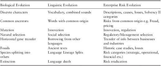
A Darwinian criteria applied to risk evolution. Based on a table by Mesoudi et al. (Reference Mesoudi, Whiten and Laland2004)
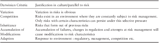
7.9 It is important to note that there are three key differences between risk and biological evolution:
1. In biological studies it is only possible to get data on species which form only a small subset of the total evolutionary data. However in risk analysis there is an advantage of being able to access all the data so long as companies are correctly identifying all their risks.
2. Risks do not exist at a given time as a varied population in which selection can act and only the fittest species survive. Instead risks have varied multiple possible future states in which ‘risk selection’ can act. It is only those risks that avoid proper management that are ‘fit’ enough to survive.
3. One element missing from risk evolution is a unit of inheritance (DNA in Biology), but it is worth noting that Darwin did not require DNA when he formulated the theory of evolution.
7.10 Nonetheless the equivalences from table 6 and table 7 allow the evolution of risk to be perceived in a similar context to standard biological evolution. This conceptual equivalence opens up the possibility of tools from evolutionary biology being successfully applied to studying risk. The next question is how are the evolutionary trees constructed using phylogenetic analysis and then how are they interpreted.
Phylogenetic Trees
7.11 Phylogenetic trees represent the evolutionary relationship between a set of taxa (in this case risks, risk scenarios or losses) based on the similarities and differences in certain characteristics of those taxa. A phylogenetic tree consists of a series of nodes that are connected by branches (see figure 38). On a phylogenetic tree the internal nodes represent hypothetical ancestors whilst the terminal nodes represent the set of taxa (risks) for which data is available. Evolution occurs independently along the branches emanating from each internal node. If at an internal node there are offspring that cannot be represented in a bifurcating pattern then a multifurcating tree is required. This occurs if one species splits off into several different lineages.
Phylogenetic trees. The tree on the left is rooted whilst the tree on the right is un-rooted. In this tree, data for nodes 1-5 was available whilst nodes 7-9 represent hypothetical ancestors. On the rooted tree, internal node 6 represents the hypothetical ancestor of all the taxa (risks); to know what this taxa may be like and its characteristic is of great interest for us to be able to understand the external taxa (risks) better

7.12 A tree may be rooted, in which case the root is the hypothetical ancestor of all the taxa in the tree. Alternatively a tree may not have a root and be un-rooted. Un-rooted trees will describe the relationship among taxa but are limited by the fact that they do not allow the entire evolutionary pathway to be seen.
7.13 The application of the phylogenetic tree approach, which is composed of nodes, and branches that link nodes, is not restricted to organisms. It can be utilised for all individual entities with taxonomic characters, such as species, populations, individuals, genes, or even organisations (McCarthy & Ridgway, Reference McCarthy and Ridgway2000), and also enterprise risks (Allan et al., Reference Allan, Yin and Cantle2010).
Constructing a Tree of Risk Evolution
7.14 The algorithms used are available in the MEGA software package. The overall tree construction process can be summarised using the following diagram in figure 39:
The basic steps for evolutionary tree construction

Preparing the data
7.15 The data will need to be in a matrix format with risks, risk scenarios or losses in rows; and with characteristics of those risks, scenarios or losses as the columns. A ‘1’ represents the presence of a character and a space or ‘0’ represents a lack of that character. An example is shown in table 8, with typical risk categories used as characters in the columns.
Typical example of a dataset for a phylogenetic analysis

7.16 There are of course times when the presence of a character is not as simple as present (1) or not (0). Although it is possible to enhance the methodology to make allowance for this, the authors find that the analysis is somewhat easier to conduct and still provides meaningful results if this subtlety is omitted. There is therefore no allowance for proportions in the methodology illustrated in this report, with a best estimate being used to determine whether a particular character is relevant to the description of a particular scenario. The rule of thumb is that if you are in doubt about a particular character, you should assume a scenario has it.
Step 1 – Produce an initial tree
7.17 The first step is to produce an approximate initial tree. For between 20 and 30 risks the “min-mini” algorithm at search level 1 will work in a reasonable amount of time (approximately less than 1 hour) but for a larger amount of risks use the “close neighbour interchange” algorithm. Use a search level of 3 and 300 random addition trees since this will increase accuracy but not significantly slow the process.
7.18 The aim of this step is only to identify groups of highly related risks and not to construct a perfect evolutionary tree. Since the algorithms used here are heuristic they should be run a few times to ensure an optimal solution.
7.19 Typically there will be a large number of equally parsimonious trees that need to be represented by a single tree. We use the ‘consense’ program for this purpose. This process is illustrated in figures 40a–e.
Output from the software showing there can be multiple trees which are equally parsimonious

Each line of output can be visualised as a tree

Other equally parsimonious trees

Output from ‘consense’ which is illustrated as a tree in figure 40e

An illustration of the tree in figure 40d and an output from ‘consense’

7.20 All these trees are then input into ‘consense’, which gives the best consensus of all the equally parsimonious trees.
7.21 The output from the ‘consense’ analysis is then shown in figure 40d, and graphically in figure 40e.
Step 2 – Identify groups of highly related risks
7.22 The next step is to use the program CTree to identify highly related risk groups. To input the data into CTree correctly, the numeric values in the ‘out-tree’ file from ‘consense’ need to be set to ‘1’.
7.23 The aim here is to find a tree root on which a more accurate algorithm can be applied. Deciding on these groups can be difficult and requires an amount of care. The groupings and rooting provided by CTree should be checked against the tree produced in the previous step to ensure that they are sensible. The software gives some guidance on this step. An example of this is shown in figures 41a–b .
CTree output marking the root of the tree with a red dot (circled) on the left

CTree output showing a rooted tree with the red dot (circled) as the root. This now gives direction to the evolution

Step 3 – Apply exact algorithms to groups of highly related risks
7.24 Apply the “max-mini branch and bound” algorithm in MEGA to each of these groups of highly related risks. This will give confidence that the evolutionary history of each of these groups is being represented as accurately as possible.
Step 4 – Combine set of solutions for each group of highly related risks
7.25 It is likely that there is still more than one ‘best’ evolutionary tree for each set of highly related risks. For further analysis combine these trees using ‘consense’. Each tree for each group of highly related risks should then be rooted as in the rooted tree produced by CTree.
Step 5 – Rejoin groups into a final tree
7.26 Each group of highly related risks should be joined together to produce a final single tree. The groups should be positioned so that this tree is of the same form as the tree produced in step 1.
Verify Evolutionary Tree
7.27 The best way to validate the tree is to check if the results are sensible from a business perspective. If it can be corroborated with other data or by someone who knows the business, then that would lend support to the conclusions.
7.28 However a couple of useful metrics do exist: the consistency index, which is a measure of how well the character data fits the evolutionary tree; and the retention index, which is a measure of common ancestry in an evolutionary tree. As a guide the retention index should be over 0.5 and the consistency index should be around the value given by the following equation
 $$Consistency\,index\, = \,0.90 - 0{\rm{.022}} \, {\rm{\ast}} \, {{N}_R}\, + \,0.000213 \, \ast \, {{({{N}_R})}^2}, $$
where NR is the number of risks in the study.
If either of these values is far from their suggested value the tree should be interpreted cautiously.
Modelling risk evolution using phylogenetic analysis
Some of the advantages of using a phylogenetic approach are:
Better Risk Classification
7.29 Early attempts to classify biological phenomena required an initial labelling process with reference to a hierarchy of criteria – not dissimilar to the way in which a typical risk classification system works today. However, biologists found this to be unsatisfactory because organisms would often share similar high level classification traits but ultimately bear little resemblance to each other. Phylogenetic analysis fundamentally differs from previous approaches in that it does not attempt to match items to a predetermined list of criteria – rather it simply looks at the characteristics of the phenomena being studied and identifies a way to group them in the simplest, most parsimonious, way.
7.30 Using phylogenetics for risk analysis provides a completely new way of looking at risk classification. By grouping risk by evolutionary history, risks no longer have to be classified as a series of similar events. Instead they can be seen as emerging from a complex system, thus allowing a unique understanding of how risks are organised.
7.31 Phylogenetic analysis removes subjectivity in risk classification using evolution as a kind of external reference point. This can be used to provide a methodology that makes clear the data, assumptions and results with the intention of making risk classification decisions transparent. It cuts across organisation boundaries and disciples and looks at risks for what they, are at an almost fundamental level and then groups them accordingly. This can be particularly useful for losses, if good loss data about individual losses is available.
Understanding Risk History
7.32 Phylogenetics can trace how risks have changed over time. This allows a much deeper understanding of the risks. Risks need no longer be seen as an event occurring now but can instead be understood by the interacting circumstances that have brought the risk into its current form. This allows companies to better understand their vulnerabilities and how to manage their risks better.
Predicting Risk Futures
7.33 Phylogenetics provides a way to use the history of risk evolution as an indication of its future evolutionary pathway. Although past corporate behaviour does not ensure an understanding of future outcomes, it provides a guide to major risk factors, and understanding the history of a risk will give glimpses as to its future. By no longer viewing risk as a fixed entity but one that varies over time, a risk's variations can be traced and its future state predicted.
7.34 Risk can change and evolve in many ways but this does appear to happen in some predictable ways. Predicting the future of the evolution of a risk will not only allow better risk mitigation but can prevent new risks from forming. From this, risks can be mitigated before they have even been fully identified as risks.
7.35 The methodology identifies small groups of highly related risks which share a common ancestor. The evolutionary history of each of the groups can then be accurately traced. By understanding the phylogeny of the risks we can:
• Determine where evolution is most prolific;
• Detail path dependency and co-evolution of risks;
• Identify the most active (evolutionary) characteristic to manage; and,
• Create focused scenarios for emerging risks modelling.
Case study – a multiline international insurance company
7.36 The case study analysis uses the same steps as discussed above and presented in figure 40.
The data used in the case-study was only a small sub-set of a wider study done for the insurer. Whilst the details of the report on the overall emerging risk exposure are confidential, we can report that the company's risk team stated that, “the procedure enabled a more realistic picture of the risk landscape to be obtained and it gave a clearer insight into how business unit's risks were developing.”
Data Preparation
7.37 Each data set consists of a matrix with risks in the rows and then 59 columns representing the possible characteristics that each risk scenario contains. The data set used in this case study consisted of different country risk registers, which has the characteristics of each risk broken down into 59 categories specified within the organisation's risk classification system.
7.38 When risk characteristics are referred to by name their number will follow in brackets. For example ‘Portfolio Risk Selection’ is character 1 and this will be written as ‘Portfolio Risk Selection’ (1). The risk codes are used for ease of labelling the trees and the coding is listed below for the 59 risk categories.
7.39 The actual pilot study project consisted of 7 different country data sets but for clarity we have selected just two, Ireland & the UK, to illustrate the phylogenetic analysis technique and interpretation. The data for Ireland and the UK are shown in tables 9 and 10 in partial form for ease of reading.
Extract of Ireland risk data showing characteristics in the columns

Extract of UK risk data

Ireland data
UK data
7.40 We have used the data to produce 2 country specific trees, Ireland and UK, as this also allows us to look across the pair of trees to look for patterns and possible co-evolution trends. The resulting evolutionary risk tree for Ireland showing clades (A, B & C) is shown in figure 42 and for the UK in figure 43 showing clades D & E.
The phylogenetic tree of risk evolution for Ireland

Risk evolution tree for UK showing clades and key risk characteristics

Ireland Tree
7.40 The numbers on the legs of the tree represent the codes of the risk characteristics (some of the key ones have been described too) that have been acquired in the evolution of that risk. A red number (circled) means a risk character has been lost in the evolution, similar to humans losing a tail in their evolution. The risks at the end of the tree legs are the risks given in the risk registers and represent the most current risks identified e.g. (IRE – 1 is Economic Downturn). The nodes represent some earlier risk that existed but has now evolved. The clades A, B & C represent clusters of at least 3 tree legs and clade-forming characters are of particular interest, which will be explained below in the discussion section.
7.41 The resulting tree for the UK is shown below in figure 43
UK Tree
Tree Verification
7.42 Two metrics are used to check whether the phylogenetic tree constructed is indeed an accurate representation of evolutionary events. The first is the consistency index, which describes how well the character data fits the phylogenetic tree. Secondly, the retention index is a measure of common ancestry in a phylogenetic tree. Both are indices between 0 and 1, with 1 being the best result. As a guide they should be above 0.5 but the consistency index has been shown to be heavily correlated to data sample size. Therefore with data sample sizes above 50 the consistency index may drop lower than this and still be an acceptable score.
7.43 The consistency index and retention index for each country are given in table 11 and represent good values:
Tree verifications

Interpretation and points to note on the risk trees
7.44 In each country the evolution of key risk characters has resulted in the formation of new risks. These key risk characters, help identify the drivers of the risks for the organisation in each country and also which risk drivers are similar across all countries. A group formed of three or more risks that can be traced back to the evolution of a single risk character is called a cladeFootnote 8. It is these clades that can provide a unique re-organisation and classification of the risks. The original risk character that forms the clade can be thought of as the key evolutionary risk character for that clade, and from that character resultant risks have already emerged.
7.45 The key characters for each country can be summed up in the following table 12. This table also identifies the key evolutionary risks that are relevant in each country.
Evolutionary traits of countries
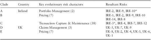
*no longer contains character
Key observations and questions
7.46 For Ireland, ‘Pricing’ (7) is the most important risk character since it defines clade B. Also important is the character ‘Portfolio Management’ (2) since this combined with ‘Pricing’ (7) to form a sub-clade (clade A) of the risks ‘IRE-2’, ‘IRE-9’ and ‘IRE-10’. What is then particularly interesting is that Pricing in the risk ‘IRE-10’, which is ‘Implementation Period Payments’, loses the character ‘Pricing’ (7), which is indicated by a red number seven.
7.47 Risks should increase in complexity and any risk that loses characters may be unstable or in a process of changing. We know from biology, and studies of viruses in particular, that losing characters can be a signal of specialisation. Again using the example of humans losing our tails, this may also be seen as a specialisation necessary to adapt to new surroundings and needs. Also one should ask the question what the risk ‘IRE -10’ would look like if it regained the pricing character. Any risk that is losing characters should be scrutinised to explain why this might be happening.
7.48 Notably, Ireland ‘IRE-1’ is quite distinct from any other risks due to its large number of characters. This is maybe to be expected from a risk like ‘Economic Downturn’ because this risk is complex and covers many areas; it could also be argued that it is too high level and should be split into more defined areas like ‘housing crises’, ‘euro crises’, etc. It is always important to look for branches with the most characters as this indicates significant evolution and where there has been evolution and much change we are likely to see more evolution.
7.49 One can argue that where there has been the most evolution is where you are more likely to see new species emerge, for example a warm jungle is host to more forms of life than the cold tundra, so you would expect more new species and more evolution in the jungle. So using this line of thought we would also be interested in ‘IRE – 7’, ‘Inadequate Data Privacy Procedures’, as it has had three branches and has many characters on the final branch. The next question would be how might it evolve? If it were to combine with ‘IRE-12’,'Immature Capability re On-line Channel’, to create a new risk what might that look like? Maybe something like the Sony Play Station data breach?
7.50 In the UK there are two clades formed from the key characters ‘Claims management’ (3) (clade D) and ‘Pricing’ (7) (clade E). Interestingly in the UK there are three risks which show no relation to any others ‘UK-11’, ‘UK-14'and ‘UK-15’. Risks that have not changed significantly are more likely to be stable; however, this should be checked against whether the risks have not been described in sufficient detail.
Comparing IRE & UK Trees
7.51 In both the UK and Ire trees the character ‘Pricing’ (7) is prominent; this might not be too surprising for an international insurance company. Comparing the tree structures we can see that Ireland has a cascading clade that has ‘portfolio management’ (2), as a key character that evolves from ‘pricing’ (7), and then ‘portfolio selection’ (1), emerging from ‘portfolio management’ (2). The UK on the other hand, has a slightly different structure but with the same characters i.e. ‘Pricing’ (7), then ‘portfolio selection’ (1), then ‘portfolio management’ (2). So what should come first in the evolution of the related risks: portfolio selection or portfolio management? This may be immaterial but the UK tree goes on to produce a risk ‘UK-1’ that is the result of another branch with a character ‘reinsurance provision’ (5). Ireland does not even seem to have this character anywhere on the tree - should it and where should it be? These would be areas for the risk manager to investigate. The visualisation of the risks and characters in a tree format enable this sort of observation to be quickly spotted that would be difficult and tiresome in a spreadsheet.
Co-evolution patterns
7.52 Looking at individual country trees and then both together we can also look for patterns of co-evolution, which means that characters or risks have a tendency to evolve in each other's presence. In nature, where co-evolution occurs, it often creates more rapid evolution and adaption e.g. a bird that develops a long beak to get nectar from a flower and the flower that continues to extend the long shape of the flower until a symbiotic dependant relationship is developed.
7.53 In the trees we have an example of risk IRE (7) ‘inadequate data privacy procedures’ that has a strong possibility that it might gain a ‘media’ (53) character because:
‘Media’ (53) only evolves in the presence of ‘Investors/JV Partners’ (52). So we can investigate risks that have character (52), but not yet (53). These conditions are found in risk IRE (7) ‘inadequate data privacy procedures’. Now couple this piece of information with the earlier warning that IRE (7) may combine ‘Inadequate Data Privacy Procedures’ and we have an interesting new risk scenario emerging.
7.54 Other patterns in the history of risk evolution can be traced and used to predict future outcomes. These are discussed in table 13:
Evolutionary patterns

8. Conclusions & Recommendations
8.1 Looking at risk management, in particular risk appetite and emerging risks, from a systemological perspective is both useful and insightful. Modern risk management is complex and ERM requires a holistic approach to make sense of the layers, interconnections and non-quantitative measures.
8.2 Our analogy of a heating system for risk appetite provides a common sense overview of the nature of the problem. The proposed integration of Concept Mapping and a Bayesian Network approach, embraces systems thinking, through looking at interconnections and integrating qualitative and quantitative measures. It has the benefits of being scalable from small/simple to large/complex but with the same underlying rigour.
8.3 It can be applied to any type of firm and can demonstrate visually to all stakeholders the impact of emerging information and new evidence. It easily accommodates expert knowledge which is then verified when data is available. As shown in the example in chapter 6, it provides a robust basis for setting and monitoring risk appetite limits and importantly is in a form that retains the interest of the relevant business professionals. It provides an easily explained narrative with evidence and a model to test scenarios that can also be used as an audit trail.
8.4 We commend this approach to the profession as a readily available methodology with robust theoretical underpinnings. Recent advances in Bayesian Network software allows for easier manipulation and visualisation of complex models. The success of the techniques, as with all models, relies on the skill and experience of the user. The skill set of the professional actuary is well suited to this approach, though some time will be required to understand and facilitate concept mapping workshops.
8.5 Emerging risk identification is a holy grail in risk management. The evolutionary approach taken in this study is novel and embraces the Darwinian concept that competition and the external environment imply constant change. This can also apply to risks, losses and indeed any organisational issue when viewed as a complex adaptive system.
8.6 The emerging risk approach uses phylogenetic theory as the means of constructing evolutionary risk trees and their interpretation. The science of phylogeny is a rapidly expanding discipline that combines biology and mathematics. New (free) software programs and algorithms allow easy access for actuaries to be able to construct their own risk trees. Interpretation of the evolutionary trees is more subjective but the detailed guidance given in the report will allow for useful insights and questions to be asked about an organisation's risk classifications, appropriate risk scenarios and potent risk characteristics.
8.7 Every organisation and industry will have unique risk trees, as each company will have had a unique history. From that platform we believe it is possible to obtain insight into what the future risks might look like and indeed what they are not likely to be. This approach is in its infancy but promises a new way of conceiving and thinking about risks and risk management more generally, particularly in an ERM context.
8.8 Feedback from the executives involved in the case studies and subsequent trials in other organisations, find the Bayesian Network approach an immediate solution to a pressing regulatory need. They find the emerging risk approach stimulated their thinking and helped them to focus on some key areas of the business under threat. In some cases the analysis confirmed intuitive thoughts and in others genuinely identified new areas for investigation.
8.9 The authors would genuinely welcome input and comments on this report.
Glossary
Agent Based Model: a type of computer simulation that models the relationships and behaviours of agents within a complex system, in order to model the emergent behaviour of the system as a whole.
ArtificialNeuralNetwork: an automated multi nonlinear regression process capable of learning.
BayesianBeliefNetworks (BBN, BeliefNetworks or BayesianNets): a directed acyclic graph (DAG) model to represent knowledge about uncertain domains.
BayesianNetworks: a system based on Bayesian probability theory that can perform inference and learning.
CellularAutomata: a discrete modelling approach to explore the behaviour of a complex system.
ChaosTheory: a mathematical theory to explain complexity, dynamics, and the nonlinearity of a system.
Cladistics: a method of classifying species of organisms into groups.
Cladogram: a diagram that shows ancestral relationships between organisms/species.
CognitiveMapping: a technique to visualise the complex and nonlinear relationships between different concepts or cognitive constructs.
ComplexAdaptiveSystems(CAS): an explanatory framework for helping people to understand complexity.
ComplexSystems: systems together with behaviour rules that cause the state of at least one of its objects to change over time.
ComplexityScience: a new field that studies universal principles common to all complex systems.
Complexity: the inter-relationship, inter-action and inter-connectivity of elements within a system and between the system and its environment.
EmergingRisks: Emerging risks are the emergence of unintended consequences as a result of complex interactions between strategic objectives, existing risks, risk management interventions, business and regulatory environment, markets and people's behaviour.
EnterpriseRiskManagement (ERM): Enterprise risk management is a process, effected by an entity's board of directors, management and other personnel, applied in strategy setting and across the enterprise, designed to identify potential events that may affect the entity, and manage risk to be within its risk appetite, to provide reasonable assurance regarding the achievement of entity objectives.
FuzzyLogic: a many-value logic dealing with fuzzy set numbers.
GeneticAlgorithm: an evolution-based approach applied for optimisation purposes.
HardSystems: those systems or problems with clearly defined goals, and missions that can be addressed via engineering methodologies in attempting to, in some sense, ‘optimise’ a solution.
NetworkTheory: the theory that deals with the application of networks.
Phylogeneticanalysis: a mathematical method to elicit evolutionary relationships.
RiskAppetite: the comfort and preference for accepting a series of interconnected uncertainties related to achieving our strategic goals.
SoftSystems: those systems or problems that are extremely complex, problematical, and often mysterious phenomena for which concrete goals cannot be established and which require learning in order to make improvement.
System: any two or more elements that are interconnected for a purpose.
System Theory: the multidisciplinary study of systems in general.
SystemicRisks: a systemic risk materialises when an initial disturbance is transmitted through the networks of interconnections that link firms, households and financial institutions with each other; leading, as a result, to either the breakdown or degradation of these networks.
SystemsDynamicModelling: an approach to model the complex interrelationships, especially the casual and nonlinear relationships, between system elements.
SystemsThinking: the process of discovery and inquiry that uses techniques to understand the interrelationships and underlying patterns of problems and opportunities.
Appendix A – Complexity Science
Hitchins (Reference Hitchins2007) proposes seven principles for this cyclical behaviour shown in figure A1. These are described below and then their relationships are shown in figure A2 in, what Hitchins describes as, a unified systems life-cycle. This can be applied to any complex system.
Cyclic progression – entropic cycling

The unified systems life-cycle

Principle of systems reactions
If a set of interacting systems is in equilibrium and either a new system is introduced to the set or one of the systems or interconnections undergoes change then, as far as they are able, the other systems will rearrange themselves so as to move to a new equilibrium.
Principle of system cohesion
Within a stable system, the net cohesive and dispersive influences are in balance. In physical systems this equates to Newton's third law and is quite obvious. It is not so obvious in social systems but groups of people, for example, are held together by social bonds whilst other forces, such as modernization, tend to separate them.
Principle of adaptation
For continued system cohesion, the main rate of systems adaptation must equal or exceed the mean rate of environmental adaptation.
Principle of connected variety
Interacting systems’ stability increase with variety and with the degree of connectivity of that variety within the system.
Principle of limited variety
Variety in interacting systems is limited by the space and the degree of differentiation.
Principle of preferred patterns
The probability that interacting systems will adopt locally stable configurations increases with both the variety of systems and their connectivity.
When these principles are combined together with the principle of entropic cycling (above in figure A1) we have the causal loop model of the unified systems life cycle as shown in figure A2.
To appreciate the model we start at the top with energy which creates variety or, rather, increases the space within which variety may manifest itself. We see this in everyday life: in the variety of cars in richer cities; in the variety of jobs in cities compared to villages; and in the variety of species in a tropical jungle compared with tundra regions.
With variety generation there is the increased opportunity for varieties to interact and to react. This may cause cooperative, symbiotic, mutually sustaining or complementary sets to form. This may be seen as connected variety, which leads to stability owing to both the potential for homeostatic balance and constructive feedback. Note there is nothing stated about the way in which this stability arises – it may be linear, chaotic or even catastrophic.
As an interacting web of systems forms, it adopts preferred patterns. Although these exhibit high energy they are generally ‘local’ energy wells, meaning that while they are high energy, they are not as high as they might otherwise be. For example, animals with a preference for certain foods such as the Giraffe's preference for leaves at the top of trees.
Preferred patterns encourage ‘systems cohesion’, the tendency of the system's elements to cohere in some way. This systems cohesion is challenged by disruptive influences. These may be things like: pathogens in the human body; increases in the base lending rate; or competition for skilled workers, etc.
There is an observable tendency for systems with complementary varieties to encourage one or more varieties to become dominant, leading and overshadowing the rest and setting rules and limits. The dominant member tends to suppress variety as this is seen, especially in times of hardship, as wasteful and superfluous.
With a reduction in variety, a system may still appear robust to an external viewer – as a forest of hardwood would appear robust. However, the system is vulnerable: when the environment changes, it will lack the variety with which to adapt and respond. In this event, the system will decay or collapse and its constituents may rejoin the pool of varieties generated by energy, so rejoining the entropic cycle at the start point.
Mills (Reference Mills2010) in his review of more than 40 different methods to measure complexity presented six that might be enlightening for actuaries:
• Transaction information: The number of bits of information required to identify the elements of a typical system transaction.
• Network complexity: There are many measures of network complexity, but a key one is the average number of connections per network vertex (node).
• Degree of hierarchy: The levels of hierarchy, or number of nested elements within a system. More complex systems have more levels.
• Algorithmic information content: The number of bits in the shortest computer program that completely describes the system.
• Logical depth: The number of steps a Turing machine would take to construct the series of 0s and 1s that completely describes a system. This is a measure of how difficult it is to construct a system.
• Statistical complexity: The minimum amount of information about a system's past behaviour required to predict its near-term future statistical behaviour.
Appendix B – Systems Thinking
Parts, Wholes and Layers
Components can be seen as being a hierarchy of holons which are anything considered, at the same time, to be both a part and a whole. An example would be person, who is part of: a family, a neighbourhood, a country etc. and yet also a whole made up of parts or sub-systems i.e. skeleton, nervous system, etc. A holon is seen to have emergent properties that derive from the co-operation of the parts. This introduces the concept of inside and outside defined by boundaries. An open system is one which continually interacts with its environment whereas a closed system can be assumed to be self-contained.
Connections
The relationships between the holons and their ability to communicate determine the emergent behaviours and unintended consequences. It is generally useful to think in terms of feedback loops which need to be used to help us to create learning and foresight to manage the processes involved.
Processes
Process may be concisely defined as ‘How change happens’. This definition includes naturally occurring change as well as anthropogenic change. Answers to the questions ‘who’, ‘what’, ‘why’, ‘where’, ‘when’ and ‘how’ enable us to describe a process. ‘Why’ identifies the purpose and hence drives the change in ‘who’, ‘what’, ‘where’ and ‘when’ through the transformations identified by ‘how’. The output of a process may be a product but that in itself has a life cycle and is also a process.
It is important to distinguish between purpose – which is the result, outcome or effect that is intended from the system – and a requirement, which is an unambiguous statement of the capability that the system must deliver. A requirement is expressed in operational terms (what the system will do) rather than solutions (how the system will do it). Purpose is the answer to the question: Why are we doing this process? It is the driver of intended change and by inference defines unintended consequences as well.
Integrating models
Models are the means by which a systems thinker comes to terms with complex real world problems. Checkland's (1999) soft systems method (figure B2) shows the basic process used.
Systems thinking – essential ideas

Using Systems models

The comparison between the real world problem situation and systems models stimulates learning and action which in turn feeds back into the learning process. It is inevitable that in complex situations the model is not a true view of the situation but it can be sufficient for its purpose. It requires judgment to determine whether something is fit for purpose.