2. Gyrokinetic model

We consider slab geometry with magnetic shear, so the magnetic field in Cartesian coordinates $(x^{\prime },y^{\prime },z^{\prime })$ is $\boldsymbol{B}=[\boldsymbol{e}_{z^{\prime }}+(x^{\prime }/L_{s})\boldsymbol{e}_{y^{\prime }}]B$ for some constant $B$ and shear length $L_{s}$ . A field-aligned coordinate system is introduced: $x=x^{\prime },y=y^{\prime }-x^{\prime }z^{\prime }/L_{s},z=z^{\prime }$ , so $\boldsymbol{B}\boldsymbol{\cdot }\boldsymbol{{\rm\nabla}}x=\boldsymbol{B}\boldsymbol{\cdot }\boldsymbol{{\rm\nabla}}y=0$ and $\boldsymbol{B}\boldsymbol{\cdot }\boldsymbol{{\rm\nabla}}z=B$ . In this geometry, we consider the nonlinear electrostatic gyrokinetic equation (Frieman & Chen Reference Frieman and Chen1982), dropping toroidal effects:

together with the quasineutrality condition

Here, $s\in \{i,e\}$ subscripts denote particle species, ${\it\Phi}(t,\boldsymbol{r})$ is the electrostatic potential, $h_{s}(t,\boldsymbol{R}_{s},\mathscr{E}_{s},{\it\mu})$ is the non-adiabatic distribution function, $\mathscr{E}_{s}=m_{s}v^{2}/(2T_{s})$ , ${\it\mu}=v_{\bot }^{2}/(2B)$ and $f_{Ms}$ is the leading-order Maxwellian. The scale length of the equilibrium density $n$ is $L_{n}=-n/(\text{d}n/\text{d}x)$ , $q_{i}=e=-q_{e}$ is the proton charge, $T_{s}$ is the species temperature, ${\it\eta}_{s}=(\text{d}\ln T_{s}/\text{d}x)/(\text{d}\ln n/\text{d}x)$ , $C_{s}$ is the collision operator, and $\langle \,\rangle _{\boldsymbol{r}}$ and $\langle \,\rangle _{\boldsymbol{R}_{s}}$ denote gyroaverages at fixed particle position $\boldsymbol{r}=(x,y,z)$ and guiding-centre position $\boldsymbol{R}_{s}=(X_{s},Y_{s},Z_{s})$ . The distinction between $z$ and $Z_{s}$ may be neglected. We consider a flux tube domain, in which the fluctuating quantities can be taken to be periodic in $x$ and $y$ . Expanding the fluctuating quantities in spatial Fourier modes as ${\it\Phi}=\sum _{k_{x},k_{y}}{\it\Phi}_{k_{x},k_{y}}(t,z)\exp (\text{i}k_{x}x+\text{i}k_{y}y)$ and $h_{s}=\sum _{k_{x},k_{y}}h_{s,k_{x},k_{y}}(t,z,\mathscr{E}_{s},{\it\mu})\exp (\text{i}k_{x}X_{s}+\text{i}k_{y}Y_{s})$ , we may replace the gyroaverages with Bessel functions: $\langle {\it\Phi}_{k_{x},k_{y}}\exp (\text{i}k_{x}x+\text{i}k_{y}y)\rangle _{\boldsymbol{R}_{s}}=J_{0s}{\it\Phi}_{k_{x},k_{y}}\exp (\text{i}k_{x}X_{s}+\text{i}k_{y}Y_{s})$ and $\langle h_{s,k_{x},k_{y}}\exp (\text{i}k_{x}X_{s}+\text{i}k_{y}Y_{s})\rangle _{\boldsymbol{r}}=J_{0s}h_{s,k_{x},k_{y}}\exp (\text{i}k_{x}x+\text{i}k_{y}y)$ , with $J_{0s}=J_{0}(k_{\bot }v_{\bot }/{\it\Omega}_{s})$ and ${\it\Omega}_{s}=eB/m_{s}$ . The perpendicular wavenumber is given by

The system is uniquely specified by the following dimensionless parameters: $L_{s}/L_{n}$ , ${\it\eta}_{i}$ , ${\it\eta}_{e}$ , $T_{e}/T_{i}$ and collisionality ${\it\nu}_{ee}L_{n}/v_{i}$ , where ${\it\nu}_{ee}=\sqrt{2}{\rm\pi}ne^{4}\ln {\it\Lambda}/[(4{\rm\pi}{\it\epsilon}_{0})^{2}m_{e}^{1/2}T_{e}^{3/2}]$ is the electron–electron collision frequency and $v_{i}=\sqrt{2T_{i}/m_{i}}$ .

It should be noticed that the parallel coordinate $z$ enters the system (2.1)–(2.3) only through (2.3). It should also be noticed that $k_{x}$ enters the system (2.1)–(2.3) only through (2.3) and through the nonlinear term in (2.1). Therefore, a linear mode at non-zero $k_{x}$ and non-zero $k_{y}$ satisfies exactly the same equations as the corresponding $k_{x}=0$ mode, but translated in $z$ by $L_{s}k_{x}/k_{y}$ . As a consequence, the linear growth or damping rates of $k_{y}\neq 0$ modes are independent of $k_{x}$ , and the eigenmode structures are independent of $k_{x}$ up to this translation in $z$ .

One important property of the system (2.1)–(2.2) is the free-energy conservation equation (Sugama et al. Reference Sugama, Okamoto, Horton and Wakatani1996; Howes et al. Reference Howes, Cowley, Dorland, Hammett, Quataert and Schekochihin2006; Abel et al. Reference Abel, Plunk, Wang, Barnes, Cowley, Dorland and Schekochihin2013) obtained by applying the operation $\sum _{s}\int \text{d}^{3}R_{s}\int \text{d}^{3}v(T_{s}h_{s}/f_{Ms})(\cdots )$ to (2.1):

where

is the free energy, ${\it\delta}f_{s}=h_{s}-q_{s}{\it\Phi}f_{Ms}/T_{s}$ is the total departure of the distribution function from a Maxwellian and

is the net energy source. (To derive (2.4)–(2.6), the equalities $\int \text{d}^{3}R_{s}\int \text{d}^{3}v\langle \cdots \rangle _{\boldsymbol{R}_{s}}=\int \text{d}^{3}R_{s}\int \text{d}^{3}v(\cdots )\approx \int \text{d}^{3}r\int \text{d}^{3}v(\cdots )=\int \text{d}^{3}r\int \text{d}^{3}v\langle \cdots \rangle _{\boldsymbol{r}}$ are used. The $v_{\Vert }\partial h_{s}/\partial z$ term in (2.1) has been integrated by parts; as detailed in Banón Navarro (Reference Banón Navarro2012, p. 66), the associated boundary term vanishes for a finite- $z$ domain using a twist-and-shift parallel boundary condition (Beer, Cowley & Hammett Reference Beer, Cowley and Hammett1995), taking the fluctuation amplitude to vanish at the ends of each set of linked domains.) The first term on the right-hand side of (2.6) is negative-definite (by the $H$ -theorem). The second term has the form of the particle and heat fluxes multiplied by the density and temperature gradients, and this term increases $W$ if the fluxes have the appropriate sign to relax the gradients. Thus, in a turbulent steady state where $W$ is statistically constant, (2.4)–(2.6) indicate that energy is injected by the equilibrium gradient(s) and dissipated by collisions. It should be noted that the operation $\int \text{d}^{3}R_{s}$ used in the derivation of (2.4) annihilates the nonlinear term in (2.1), and so (2.4)–(2.6) apply to both the linear and nonlinear dynamics.

The system (2.1)–(2.2) may or may not possess absolute linear instability, depending on the physical parameters. For the rest of this paper, we take ${\it\eta}_{i}={\it\eta}_{e}=0$ , so it is certain that the ITG and electron-temperature-gradient (ETG) instabilities are suppressed. Even without temperature gradients, the system may still be unstable to the universal instability driven by the density gradient. For reference, the growth rates and frequencies of this instability in the absence of magnetic shear are given in appendix A. As detailed in appendix A, some insight into the instability can be obtained by expanding the plasma dispersion function $Z$ for the electrons in the small-argument limit, $Z({\it\omega}/(|k_{\Vert }|v_{e}))\approx \text{i}\sqrt{{\rm\pi}}$ for $|{\it\omega}/(k_{\Vert }v_{e})|\ll 1$ , and by expanding the ion $Z$ function in the large-argument limit, $Z({\it\omega}/(|k_{\Vert }|v_{i}))\approx -|k_{\Vert }|v_{i}/{\it\omega}$ for $|{\it\omega}/(k_{\Vert }v_{i})|\gg 1$ . One then finds a frequency with positive imaginary part $\propto \text{i}\sqrt{{\rm\pi}}/L_{n}$ , indicating that the instability is due to resonant electrons in the presence of a density gradient. When an arbitrarily small amount of magnetic shear is introduced, the global eigenmodes are no longer recognizable as the unsheared slab modes, and indeed are absolutely stable for $k_{y}{\it\rho}_{i}\ll 1$ (Ross & Mahajan Reference Ross and Mahajan1978; Tsang et al. Reference Tsang, Catto, Whitson and Smith1978). One might reasonably expect weakly sheared systems with stable global eigenmodes to exhibit transient linear amplification, with the number of $e$ -foldings of amplification tending to infinity as the magnetic shear tends to zero. In the following section, we will show this hypothesis to be true, and thereby demonstrate the apparently singular limit of zero shear to be a continuous limit of the general shear case.

3. Transient linear amplification

Turning now to linear initial-value simulations, we indeed find that significant transient linear amplification is possible for certain parameters. Figure 1(a) illustrates a linear computation for a single $(k_{x},k_{y})$ in a case of very weak magnetic shear, $L_{s}/L_{n}=300$ . Other parameters used are $k_{y}{\it\rho}_{i}=1$ (where ${\it\rho}_{i}=v_{i}/{\it\Omega}_{i}$ ), ${\it\nu}_{ee}L_{n}/v_{i}=0.05$ , $m_{i}=3672m_{e}$ , $T_{e}=T_{i}$ and ${\it\eta}_{i}={\it\eta}_{e}=0$ . The results are independent of $k_{x}$ up to a translation in $z$ , as noted previously. Collisions are also included to eliminate absolute instability for $k_{y}{\it\rho}_{i}\geqslant 0.7$ , as discussed in Landreman et al. (Reference Landreman, Antonsen and Dorland2015), using the collision operators detailed in Abel et al. (Reference Abel, Barnes, Cowley, Dorland and Schekochihin2008). As transient amplification generally depends on the choice of norm, here we compare three reasonable quadratic norms: $W$ , $\int \text{d}z\,|{\it\Phi}|^{2}$ and the maximum of $|{\it\Phi}|^{2}$ along $z$ . The curve for each norm is scaled by a constant so that the initial amplitude is one. Amplification by several orders of magnitude is observed in all norms before exponential decay sets in.

For the calculation in figure 1, the initial condition used is the standard ‘noise’ initial condition of gs2: $g_{s}=h_{s}-\langle {\it\Phi}\rangle _{\boldsymbol{R}_{s}}q_{s}f_{Ms}/T_{s}$ is set to a Maxwellian velocity distribution times a random complex number at each grid point in $z$ . (The real and imaginary parts of these complex numbers are each taken from a uniform distribution on $[-1,1]$ .) While techniques exist to calculate the optimal perturbation that gives maximum amplification (Farrell & Ioannou Reference Farrell and Ioannou1996; Squire & Bhattacharjee Reference Squire and Bhattacharjee2014a ,Reference Squire and Bhattacharjee b ), such techniques are numerically challenging for this kinetic model due to the high dimensionality of the problem. The noise initial condition is a convenient shortcut, ensuring that energy is likely to be given to a growing perturbation if one exists. It has been shown in Camargo et al. (Reference Camargo, Tippett and Caldas1998) and Squire & Bhattacharjee (Reference Squire and Bhattacharjee2014b ) that for studies of transient linear amplification, random initial conditions represent a reasonable proxy for a directly calculated optimal initial condition. Figure 1(b) shows that when the calculation is repeated many times, the dynamics of the energy in figure 1(a) is typical.

Results for the three norms shown in figure 1(a) are quite similar, although the curve for the $W$ norm appears slightly higher than the other curves due to less decay in the initial period $tv_{i}/L_{n}<20$ . Indeed, we find that all results described or plotted for the remainder of this paper are quite similar for all of these norms, using the locally Maxwellian initial perturbations described above. However, there are certain non-Maxwellian initial perturbations that can cause arbitrarily fast growth in the electric field energy norms but not in the $W$ norm (Hammett, G. W. & Abel, I. G. 2015, Personal Communication). Furthermore, it is $W$ that is conserved by the nonlinearities (recall the conservation equation (2.4)), and thus the $W$ norm that plays a role in determining bounds on the possibility of nonlinearly sustained turbulence, as we will show in § 5. For these reasons, we henceforth restrict our attention to the $W$ norm.

Figure 1.

(a) Linear evolution for $L_{s}/L_{n}=300$ , ${\it\eta}_{i}={\it\eta}_{e}=0$ , ${\it\nu}_{ee}=0.05v_{i}/L_{n}$ and $k_{y}{\it\rho}_{i}=1$ , illustrating transient amplification in three norms. The initial conditions are detailed in the main text. (b) On repeating the calculation 50 times, the results are always qualitatively similar. (c) The amount of transient amplification may be defined relative to $t=0$ or relative to the minimum that occurs shortly thereafter. (d) The potential structure along a field line for this example.

Figure 1(c) shows the same computation, zooming in to the initial transient period. Before the amplification begins around $tv_{i}/L_{n}=20$ , there is an initial decay period due to strongly damped modes. An amplification factor may be defined either relative to this minimum amplitude or relative to the amplitude at $t=0$ . In both cases, we define the amplification factor to be 1 if there is no such transient amplification.

The transiently growing structures in the presence of magnetic shear are related to the zero-shear eigenmodes. To demonstrate this relationship, we consider a single $(k_{x},k_{y})$ , and define an effective $k_{\bot }$ at each time for the transient fluctuation by

Similarly, we define an effective $|k_{\Vert }|$ at each time for the transient structure by

where $\tilde{{\it\Phi}}_{k_{x},k_{y}}$ is the Fourier transform of ${\it\Phi}_{k_{x},k_{y}}$ in $z$ . Using these effective values of $k_{\bot }$ and $k_{\Vert }$ , the zero-shear dispersion relation may be evaluated. The resulting growth rate and real frequency can then be compared with the behaviour of the finite-shear transient structure. An example of such a comparison is given in figure 2, using the same simulation as in figure 1. For this case, we evaluate $\langle k_{\bot }\rangle$ and $\langle |k_{\Vert }|\rangle$ at $t=300L_{n}/v_{i}$ . The figure shows that near this time, in the region $z\approx 300L_{n}$ where the transient structure has greatest amplitude, the transient does resemble a wave packet with the real frequency and growth rate of the zero-shear eigenmode evaluated at $\langle k_{\bot }\rangle$ and $\langle |k_{\Vert }|\rangle$ . The zero-shear eigenmodes cannot remain true eigenmodes when even a minute amount of magnetic shear is introduced, since introducing shear turns $k_{\bot }$ from a constant into a function of $z$ . However, if this variation of $k_{\bot }(z)$ is on a longer scale length than ${\sim}1/k_{\Vert }$ of the perturbation, then a localized wave packet can exist in a region of nearly constant $k_{\bot }$ . We can then expect the zero-shear dispersion relation to give accurate predictions for the central frequency and growth rate of the packet. This packet will move in $z$ , and as a result, the central values of $k_{\bot }$ and $k_{\Vert }$ will evolve, meaning that the equivalent zero-shear eigenmode at one time will differ from the equivalent zero-shear eigenmode at another time. Since the frequency and growth rate of the finite-shear structure thus evolve in time, this structure is not itself a true eigenmode; the true eigenmode is only established once all points along the field line have had time to communicate with each other. However, at each instant of the transient growth phase, the finite-shear structure grows at precisely the rate expected from the zero-shear instability at the average wavenumbers $\langle k_{\bot }\rangle$ and $\langle |k_{\Vert }|\rangle$ .

Figure 2.

Comparison of the finite-shear transient from figure 1 with a zero-shear eigenmode, where $k_{\bot }$ and $k_{\Vert }$ for the latter are chosen to be $\langle k_{\bot }\rangle$ and $\langle |k_{\Vert }|\rangle$ from the transient at $t=300L_{n}/v_{i}$ . It can be seen that near this time, the transient resembles a wave packet with roughly the same complex frequency as the zero-shear eigenmode. (The amplitude and phase of the eigenmode in (b) are arbitrary.)

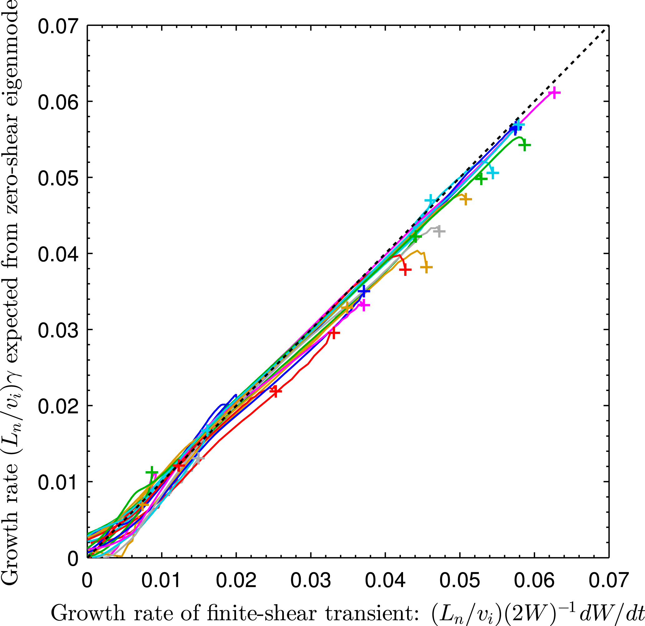
To demonstrate this principle across a range of parameters, figure 3 shows that the correspondence between the finite-shear transients and zero-shear eigenmodes is maintained throughout the evolution of the transient, for a range of values of magetic shear. In this figure, we display 25 independent simulations of linear transients, varying $L_{s}/L_{n}$ between 20 and 300, and plotting the evolution of ${\it\gamma}=(2W(t))^{-1}\,\text{d}W/\text{d}t$ from the time of peak growth rate to the time at which the energy begins to decay. For all simulations shown, $k_{y}{\it\rho}_{i}=2$ and ${\it\nu}_{ee}=0.05v_{i}/L_{n}$ . Both $\langle |k_{\Vert }|\rangle$ and $\langle k_{\bot }\rangle$ increase with time during the transient growth, corresponding to movement upward and rightward in figure 10(a). As a result, the effective zero-shear growth rate decreases over time. For all transients we examined, there is very close agreement between the instantaneous growth rate of the transient and the ‘predicted’ growth rate from the zero-shear dispersion relation. Thus, we can conclude that the transiently growing structures are closely related to the zero-shear eigenmodes.

Figure 3.

Although a change from zero to small finite magnetic shear causes a fundamental change in the eigenvalues (which change from unstable to decaying), the transient finite-shear structures retain a similarity to the zero-shear modes. As shown here, the instantaneous growth rate of the transient finite-shear structure is nearly identical to the growth rate of a zero-shear eigenmode at the dominant $k_{\bot }$ and $k_{\Vert }$ values (3.1)–(3.2). Each trajectory shown is an independent linear initial-value calculation, with $L_{s}/L_{n}$ varying from 20 to 300 between simulations. The growth rate is plotted from the time of maximum growth rate (at the $+$ symbols) until decay begins.

For the range of $k_{\Vert }$ and $k_{\bot }$ values computed for the transient structures of figure 3, the zero-shear dispersion relation is well approximated by the approximate analytic dispersion relation (A 2). Thus, we can also conclude that the transient structures, like the zero-shear eigenmodes, are driven by the combination of resonant electrons and the density gradient.

In contrast to the agreement shown in figure 3 for the amplification phase following the maximum growth rate, we do not find such close agreement between the zero-shear dispersion relation and the finite-shear dynamics for very early times, before the maximum growth rate occurs. In this initial period, a single dominant wave packet has not yet overtaken other fluctuations present in the initial random noise. We also do not see such close agreement between the zero-shear and finite-shear behaviour during the decay phase of the latter, i.e. at large times. The finite-shear decay rate as $t\rightarrow \infty$ corresponds to an eigenvalue, and it was established in previous work (Antonsen Reference Antonsen1978; Ross & Mahajan Reference Ross and Mahajan1978; Tsang et al. Reference Tsang, Catto, Whitson and Smith1978) that the finite-shear eigenvalues are not continuously related to the zero-shear eigenvalues. In an eigenmode, points at all $z$ have a coherent time dependence. Thus, this damping rate is determined by a coherent interaction between points of different $k_{\bot }(z)=k_{y}\sqrt{1+(z/L_{s})^{2}}$ , and between all $k_{\Vert }$ Fourier components. This damping rate is thus not well approximated by the zero-shear dispersion relation which assumes a single $k_{\bot }$ and single $k_{\Vert }$ .

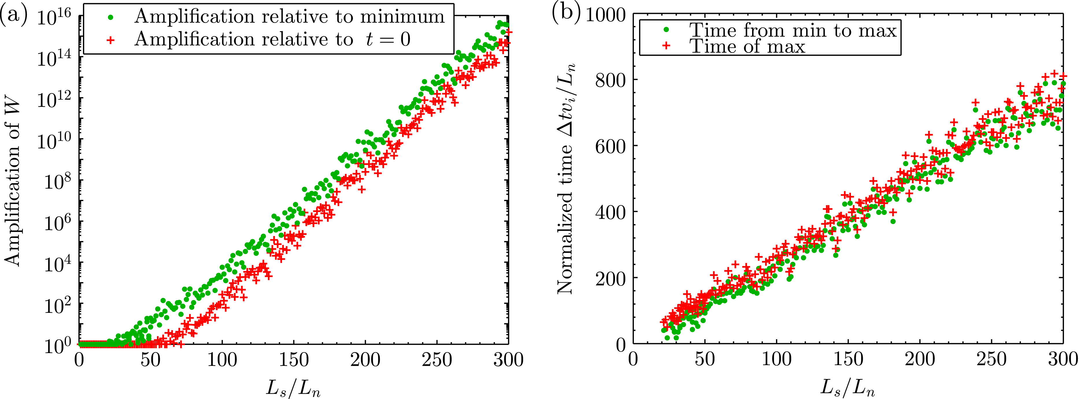
Transient amplification is exponentially reduced by increasing magnetic shear, as illustrated in figure 4. For this figure, $k_{y}{\it\rho}_{i}$ is fixed at 2, and other parameters are the same as in figure 1. (We choose $k_{y}{\it\rho}_{i}=2$ here since wavenumbers near this value will turn out to be the most amplified, as we will find shortly.) There is some scatter in figure 4, associated with the random initial condition, but the exponential trend with $L_{s}/L_{n}$ is clear. It should be noticed that amplification only appears to be possible if $L_{s}/L_{n}\gtrsim 20$ . Values of $L_{s}/L_{n}$ far in excess of 20 are obtained in the edge of tokamak experiments. (For a high-aspect-ratio tokamak, $L_{s}\sim qR/{\hat{s}}$ , where $q$ is the safety factor, $R$ is the major radius, ${\hat{s}}=(r/q)\,\text{d}q/\text{d}r$ and $r$ is the minor radius.) Figure 4(b) demonstrates that the time over which amplification occurs varies approximately linearly with $L_{s}/L_{n}$ . The figure compares two measures of the duration of amplification, measuring to the time of maximum either from $t=0$ or from the time of minimum $W$ , akin to figure 1(b) but in the time coordinate. These two measures of amplification duration display a similar linear trend.

While figures 2 and 3 made the case that the transients are insensitive to shear in one sense, it is not a contradiction that the transients are sensitive to shear in the sense of figure 4(a,b). Figures 2 and 3 show that the dominant complex frequency of the transient at each instant depends on time only through $\langle k_{\bot }\rangle (t)$ , $\langle |k_{\Vert }|\rangle (t)$ and the zero-shear dispersion relation, with no significant additional dependence on shear. However, $\langle k_{\bot }\rangle (t)$ and $\langle |k_{\Vert }|\rangle (t)$ are sensitive to shear, yielding the sensitivity of the overall $W(t)$ curve for each transient seen in figure 4(a,b).

Figure 5 shows the dependence of the amplification factor on $k_{y}$ at fixed $L_{s}/L_{n}=200$ . Significant amplification can be observed for a range of $k_{y}$ surrounding $1/{\it\rho}_{i}$ . Results are shown for two values of collisionality, ${\it\nu}_{ee}L_{n}/v_{i}=0.1$ and $0.5$ . (When the collisionality is much smaller than these values, absolute linear instability is present (Landreman et al. Reference Landreman, Antonsen and Dorland2015).) It can be seen that increasing collisionality tends to limit amplification at larger $k_{y}$ , while having much less effect at smaller $k_{y}$ . This kinetic problem is similar to conventional hydrodynamics in that for both cases non-modal amplification decreases with increasing collisional dissipation (associated with viscosity in the Navier–Stokes equation for the hydrodynamic case).

Figure 4.

(a) The number of $e$ -foldings of transient amplification and (b) the duration of the amplification both scale with the magnetic shear length scale $L_{s}$ , consistent with the appearance of absolute instability in the limit of vanishing shear ( $L_{s}\rightarrow \infty$ ). The parameters used are $k_{y}{\it\rho}_{i}=2$ and ${\it\nu}_{ee}=0.05v_{i}/L_{n}$ .

Figure 5.

Transient amplification can be observed for a range of $k_{y}$ surrounding $1/{\it\rho}_{i}$ . For this figure, $L_{s}/L_{n}=200$ . The two collisionalities shown are ${\it\nu}_{ee}L_{n}/v_{i}=0.1$ and $0.5$ .

In the context of sheared flows in neutral fluids, a relationship between transient growth and eigenvalue sensitivity has been formally proved using the notion of a pseudospectrum (Reddy & Henningson Reference Reddy and Henningson1993; Trefethen et al. Reference Trefethen, Trefethen, Reddy and Driscoll1993; Trefethen & Embree Reference Trefethen and Embree2005). The ${\it\epsilon}$ -pseudospectrum of a linear operator can be defined as the union of the sets of eigenvalues obtained when the operator is perturbed by any other operator of norm ${\leqslant}{\it\epsilon}$ , providing a precise notion of the sensitivity of eigenvalues. One can rigorously bound the amount of possible transient growth by the extent of the pseudospectrum into the unstable half of the complex plane (Reddy & Henningson Reference Reddy and Henningson1993), summarized in equation (12) of Trefethen et al. (Reference Trefethen, Trefethen, Reddy and Driscoll1993). However, for the universal instability, it is not clear that changing the magnetic shear from 0 to a small finite value has the form of the operator perturbation used to define the pseudospectrum. The reason is that the $z$ domain is infinite, and for any non-zero shear, there is always some $z$ for which the argument of $J_{0}$ is changed significantly compared with the zero-shear case. Indeed, all evidence suggests that when the shear changes from 0 to any small finite value, the eigenvalues (for a range of $k_{y}$ ) change from unstable to stable discontinuously rather than continuously (Ross & Mahajan Reference Ross and Mahajan1978; Tsang et al. Reference Tsang, Catto, Whitson and Smith1978). Thus, it may or may not be possible to understand the role of magnetic shear in the universal instability using the formal theory of pseudospectra, and we leave this careful mathematical analysis for future work.

4. Turbulence

We now demonstrate that when the nonlinear term in (2.1) is retained, sustained turbulence is possible in this system. For the demonstration here we consider the parameters $L_{s}/L_{n}=20$ , $T_{e}=T_{i}$ , $m_{i}=3672m_{e}$ , ${\it\eta}_{i}={\it\eta}_{e}=0$ and ${\it\nu}_{ee}L_{n}/v_{i}=0.05$ . We find that this point in parameter space is approximately on the edge of where sustained turbulence is possible: if the magnetic shear or collisionality is increased much beyond these values, turbulence cannot be sustained indefinitely (though it may persist for a finite time). It should be noted that $L_{s}/L_{n}=20$ is also approximately the maximum shear in figure 4 for which transient linear amplification is observed for random initial conditions. (While absolute linear instability was found in Landreman et al. 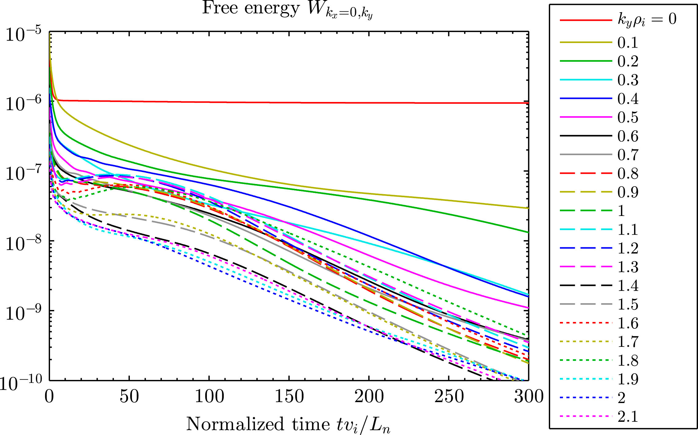(Reference Landreman, Antonsen and Dorland2015) for $L_{s}/L_{n}\geqslant 17$ in the limit of vanishing collisionality, here the finite collisionality is enough to suppress this linear instability.) Before presenting nonlinear simulations, we first illustrate the linear behaviour of the system using all the physical and numerical parameters that will be used for the nonlinear runs. Figure 6 shows the time evolution of $W$ for all the dealiased $k_{y}$ modes that will be used for nonlinear simulations, including twist-and-shift boundary conditions, but with the nonlinearity turned off, and using the random initial conditions described in § 3. More precisely, the quantities plotted are $W_{k_{x},k_{y}}$ , summed over the $k_{x}$ that link to $k_{x}=0$ , where

are the 2D Fourier contributions to $W=\sum _{k_{x},k_{y}}W_{k_{x},k_{y}}$ . Here, $L_{x}$ and $L_{y}$ are the sizes of the simulation domain in $x$ and $y$ , and ${\it\delta}f_{s}=\sum _{k_{x},k_{y}}{\it\delta}f_{s,k_{x},k_{y}}\exp (\text{i}k_{x}x+\text{i}k_{y}y)$ . Curves for the other $k_{x}$ in the simulation look similar to those in figure 6, as expected from the $z$ -translation symmetry of the system (2.1)–(2.2); see the discussion following (2.3). The amplitude of each of these curves decreases for large $t$ , confirming that there is no instability for these physical and numerical parameters. The decrease is mostly monotonic, but there is typically a small amount of transient growth by a factor of ${\lesssim}2\times$ for $k_{y}{\it\rho}_{i}$ between 1 and 2. Thus, this point in parameter space is on the edge of the region in which transient linear amplification occurs, as anticipated from figure 4.

Throughout this section, the numerical parameters used are as follows: $12\times 2$ grid points in pitch angle and $\text{sgn}(v_{\Vert })$ , 12 grid points in energy, 24 grid points per cell in $z$ (with cells at $k_{y}=j{\rm\Delta}k_{y}$ linked if separated in $k_{x}$ by $4j{\rm\Delta}k_{x}$ for each integer $j\geqslant 1$ ), Courant–Friedrichs–Lewy (CFL) number 0.5, $256\times 64$ modes in $x$ and $y$ before dealiasing and box size $(L_{x},L_{y},L_{z})=(31.4{\it\rho}_{i},62.8{\it\rho}_{i},160L_{n})$ . It was verified that both the linear and nonlinear results reported in this section were not significantly altered under factor-of-2 changes in any of these numerical parameters.

One noteworthy linear property apparent in figure 6 is that damping of modes with $k_{y}=0$ is very weak, nearly invisible on the scale of the figure. Linear modes with $k_{y}=0$ and $\partial /\partial z=0$ are damped only by collisions. (In the absence of any collisions, any $h_{e}$ and $h_{i}$ that depend only on $\mathscr{E}_{s}$ and ${\it\mu}$ are steady-state solutions of the linearized system.) Collisions introduce damping of these $k_{y}=0$ modes, with a damping rate that increases with $k_{x}^{2}$ due to the classical transport terms in the gyroaveraged collision operator.

Figure 6.

Linear dynamics for the parameters used in the nonlinear simulations of figure 7. The large- $t$ behaviour demonstrates that there is no absolute linear instability. A small amount of transient amplification can be seen.

Finally, figure 7 shows two nonlinear simulations for the same parameters as figure 6, differing only in the initial amplitude of the $k_{y}=0.1$ part of the perturbation. For sufficiently large initial amplitude, turbulence is sustained, demonstrating nonlinear instability.

A variety of strategies can be used to initiate the nonlinear instability in numerical simulations. Large-amplitude noise can be used, but this method is numerically inconvenient (at least in gs2) due to the rapid drop in amplitude of strongly damped modes over the first few time steps, which causes significant changes in the CFL-stable time step associated with the perpendicular $\boldsymbol{E}\times \boldsymbol{B}$ speed, thereby requiring recomputation of the implicit time-advance operator. Another method for initiating the nonlinear instability is to begin with a sufficient temperature gradient to bring about linear instability, and then to reduce the temperature gradient once the turbulence reaches a sufficient amplitude (Drake et al. Reference Drake, Zeiler and Biskamp1995). A third effective method, the one used in figure 7, is to initialize with one of the least damped linear eigenmodes scaled up to appropriate amplitude, with noise in the other modes. We find this method to be particularly convenient since variation in the stable time step is minimized. (In both simulations shown in figure 7, the $k_{y}{\it\rho}_{i}=0$ Fourier component is initialized to 0, but this component and the $k_{y}{\it\rho}_{i}=\pm 0.2$ components grow up quickly for the following reason. Since observable quantities are real, there is a large $k_{y}{\it\rho}_{i}=-0.1$ Fourier component present in the initial condition which is the complex conjugate of the large $k_{y}{\it\rho}_{i}=+0.1$ component shown, and these two components interact nonlinearly to drive components at the sum and difference wavenumbers.)

Figure 7.

Two simulations for exactly the same physical and numerical parameters as the decaying linear simulation in figure (6), but now including nonlinearity and varying the initial amplitude of the $k_{y}=0.1$ component. (a) When the initial amplitude is sufficient, turbulence grows and is sustained, whereas (b) for small initial amplitude, all modes decay as they do in a linear simulation.

As another demonstration that the system displays nonlinear instability without linear instability, figure 8 shows the result of turning off the nonlinear term after a period of saturated turbulence. The nonlinear term is turned off at time $tv_{i}/L_{n}=2064$ , shown as a vertical dotted line. All modes eventually decay. However, some modes display a modest amount ( ${\lesssim}3\times$ ) of transient amplification before decaying.

Figure 8.

Demonstration of the concepts in § 5. The curves show the free energy in the 2D modes with $k_{x}=0$ (including intervals linked by the twist-and-shift parallel boundary condition) for various $k_{y}$ . After a period of saturated turbulence, the nonlinear term is turned off at normalized time 2064, denoted by the vertical dashed line. All modes eventually decay, but transient amplification is apparent first for some of the 2D modes. Such amplification must occur in at least one 2D mode in such a linear ‘restart’ from steady turbulence, as proved in § 5.

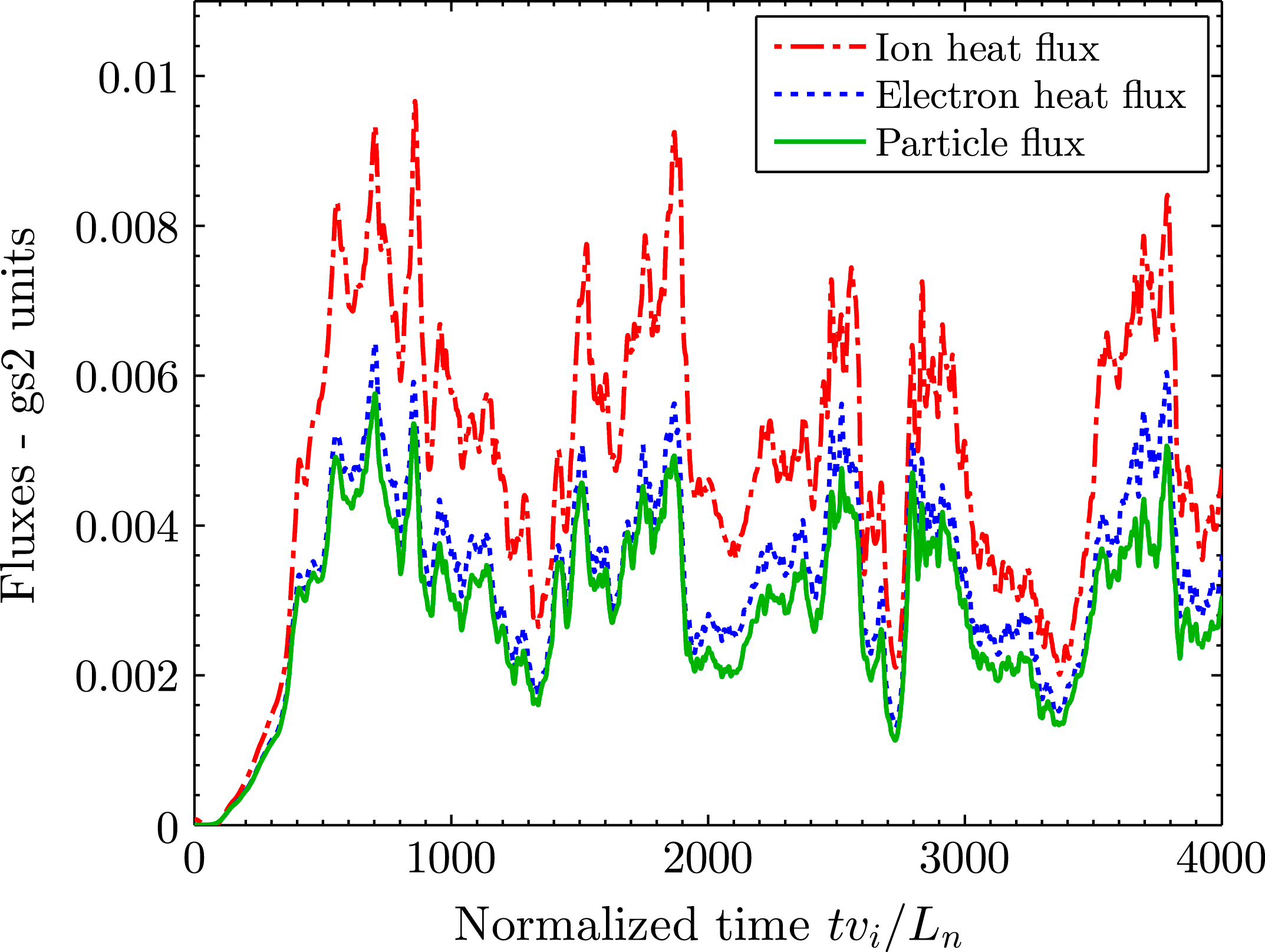
The particle and heat fluxes for a long nonlinear simulation at these parameters are plotted in figure 9. As the time average of $S$ in (2.4)–(2.6) must vanish, and since the collision term in (2.6) is negative-definite, there must be an average particle flux in the appropriate direction to relax the equilibrium density gradient, and indeed we find such a flux. Although there is no equilibrium temperature gradient, non-zero average fluxes of both ion and electron heat are found. Both heat fluxes have the same sign as the particle flux, meaning that heat flows in the $-\boldsymbol{{\rm\nabla}}n$ direction.

The fluxes in figure 9 are normalized by gyro-Bohm values defined using the length $L_{n}$ and including the two in the thermal speed, e.g. the particle flux is normalized by $({\it\rho}_{i}/L_{n})^{2}nv_{i}$ . Converting to dimensional units for a deuterium plasma, we obtain the following estimate for the turbulent particle diffusivity: $D\approx (0.4~\text{m}^{2}~\text{s}^{-1})(T/500~\text{eV})^{3/2}(B/2~\text{T})^{-2}(L_{n}/1~\text{cm})^{-1}$ . This magnitude of diffusion coefficient may be large enough to be of interest experimentally. A larger diffusion coefficient is obtained if $L_{s}/L_{n}$ is increased.

Figure 9.

Fluxes for the simulation of figure 7(a) with ${\it\nu}_{ee}L_{n}/v_{i}=0.05$ and $L_{s}/L_{n}=20$ , approximately the maximum shear at which turbulence can be sustained at this collisionality. Even in the absence of equilibrium temperature gradients, non-zero average ion and electron heat fluxes are obtained.

As mentioned earlier, for certain values of shear, collisionality and initial perturbation amplitude, a third type of behaviour was sometimes observed besides the two outcomes shown in figure 7: turbulence resembling figure 7(a) can persist for a finite time but eventually decay linearly as in figure 7(b). This finite-lifetime plasma turbulence is reminiscent of turbulent puffs in neutral (Navier–Stokes) pipe flow. In neutral pipe flow it has been found (Hof et al. Reference Hof, Westerweel, Schneider and Eckhardt2006; Tél & Lai Reference Tél and Lai2008) that in fact the lifetime of turbulence puffs does not become infinite at a critical value of the relevant physical parameter (Reynolds number), but rather the lifetime varies with the Reynolds number exponentially, so the turbulence lifetime can become longer than any reasonable observation time. An interesting open question (which we leave for future research) is whether a similar scaling of the turbulence lifetime may be present in the plasma system we consider here.

5. Turbulence implies transient amplification of typical states

It seems plausible that the previous two sections are related, i.e. that a connection exists between transient linear amplification and sustained nonlinear turbulence. Let us now prove this relationship rigorously. Here, we present two such arguments, both of which yield the conclusion that non-modal amplification is a necessary condition for sustained turbulence. One argument for the case of hydrodynamics was given in DelSole (Reference DelSole2004b ) and § 4 of DelSole (Reference DelSole2004a ), and below we adapt this reasoning to gyrokinetics. Before we do so, we give an alternative argument that relies less on linear algebra. For this discussion, it is useful to define a ‘2D mode’ to be any structure with given $k_{x}$ and $k_{y}$ , but with no restriction on the $z$ dependence (so that the structure need not be an eigenmode).

Roughly speaking, the upshot of this argument is that we should not be surprised that there is transient amplification after the nonlinear term is turned off in figure 8. Such amplification must occur. Put another way, a necessary condition for turbulence (in the absence of linear instability) is that typical states of the turbulence can be transiently amplified. Furthermore, the energy growth in the 2D modes that are amplified must be sufficient to balance the energy decay from the damped 2D modes.

We note that while $\text{d}W/\text{d}t$ is continuous when the nonlinear term is turned off, each $\text{d}W_{k_{x},k_{y}}/\text{d}t$ is generally not. The reason is that in order to annihilate the nonlinear term in the derivation of (2.4)–(2.6), it is necessary to integrate over $x$ and $y$ , i.e. sum over $k_{x}$ and $k_{y}$ . Thus, while (2.4) is identical for the nonlinear and linear dynamics, the analogous equation for $\text{d}W_{k_{x},k_{y}}/\text{d}t$ is different for the nonlinear and linear dynamics. Removal of the nonlinear term therefore causes a discontinuous change in $\text{d}W_{k_{x},k_{y}}/\text{d}t$ .

Next, we present a second argument for the necessity of transient amplification. This argument is based on linear algebra and closely follows DelSole (Reference DelSole2004b ). For this second approach, we let $\boldsymbol{h}$ denote a column vector that specifies the state of the system $\{h_{i},h_{e}\}$ in some convenient basis. For example, $\boldsymbol{h}$ could represent the array of values specifying the distribution function in a code.

Thus, we have shown in two ways that transient linear amplification is a necessary condition for turbulence in the associated nonlinear system. We have also shown that the transiently growing state(s) must have a significant amplitude in the turbulent state, in the following senses. In the first line of argument, not only must there be at least a single growing 2D mode, but there must be enough growing 2D modes of sufficient amplitude to balance the negative $\text{d}W_{k_{x},k_{y}}/\text{d}t$ of all the decaying 2D modes. In the second argument, in (5.5) there must not only be at least one state $j$ with an instantaneous growth rate ${\it\lambda}_{j}>0$ , but the amplitudes of states with positive and negative ${\it\lambda}_{j}$ must be in balance so that $\langle \text{d}W/\text{d}t\rangle =0$ . In a statistically steady state, there must be a balance between energy input from the instantaneously growing linear states and energy extraction from the instantaneously decaying linear states.

Both of the arguments above rely on the fact that the norm $W$ satisfies the same equation (2.4) in both the linear and nonlinear dynamics. Thus, the ‘nonlinear invariant’ $W$ is a special norm, and the arguments do not generally apply to other norm-like quantities such as $\int \text{d}^{3}r|{\it\Phi}|^{2}$ in which one might choose to measure transient amplification. (In fact, for any operator with damped eigenmodes, even if transient amplification exists in one norm, another norm always exists in which transient amplification is impossible. The sum of squared eigenmode coefficients is such a norm (Farrell & Ioannou Reference Farrell and Ioannou1993).)

While the arguments here rely on the gyrokinetic conservation law (2.4), the same reasoning may be applied to other models and systems in which an energy conservation equation holds. For example, equation (6) in Drake et al. (Reference Drake, Zeiler and Biskamp1995) gives the appropriate conservation law for the fluid model in that work, and the first line of (6) gives the associated norm to use in place of $W$ .

6. Discussion and conclusions

The ‘universal mode’ system (slab geometry with a density gradient, electrostatic, no sheared equilibrium flow and weak temperature gradients) is known to have a dramatic change in linear stability as the magnetic shear is raised from zero to small finite values (Antonsen Reference Antonsen1978; Ross & Mahajan Reference Ross and Mahajan1978; Tsang et al. Reference Tsang, Catto, Whitson and Smith1978; Landreman et al. Reference Landreman, Antonsen and Dorland2015). As the eigenvalues are so sensitive to magnetic shear, we might expect traditional modal analysis to give a misleading picture of typical behaviour, as with other systems that have sensitive eigenvalues (Trefethen & Embree Reference Trefethen and Embree2005). Indeed, here we have demonstrated that significant transient linear amplification is possible in the drift wave system even when all eigenmodes are decaying. As shown in figure 3, the transient structures grow at the zero-shear growth rate, when evaluated at the dominant $k_{\bot }$ and $k_{\Vert }$ at that instant. We have demonstrated that the amount and duration of amplification scale with the magnetic shear length $L_{s}$ , so these quantities naturally become unbounded in the limit of vanishing shear. The non-modal amplification also decreases with increasing collisionality, particularly at the shortest perpendicular wavelengths, and the amplification tends to be largest at wavelengths near $k_{y}{\it\rho}_{i}\sim 1{-}2$ . In contrast to more famous examples of non-modal amplification from hydrodynamics (Trefethen et al. Reference Trefethen, Trefethen, Reddy and Driscoll1993), and to some recent examples from plasma physics (Highcock et al. Reference Highcock, Barnes, Schekochihin, Parra, Roach and Cowley2010; Newton et al. Reference Newton, Cowley and Loureiro2010; Barnes et al. Reference Barnes, Parra, Highcock, Schekochihin, Cowley and Roach2011; Schekochihin et al. Reference Schekochihin, Highcock and Cowley2012), the amplification in the plasma drift wave system here does not depend on sheared equilibrium flow.

We have also demonstrated using nonlinear gyrokinetic simulations that sustained turbulence is possible in this system even when all linear modes are damped. This phenomenon had been seen previously in fluid models (Scott Reference Scott1990, Reference Scott1992; Drake et al. Reference Drake, Zeiler and Biskamp1995). This phenomenon, clearly visible in figure 7, is opposite to the ‘Dimits shift’ (Dimits et al. Reference Dimits, Bateman, Beer, Cohen, Dorland, Hammett, Kim, Kinsey, Kotschenreuther, Kritz, Lao, Mandrekas, Nevins, Parker, Redd, Shumaker, Sydora and Weiland2000) seen at different physical parameters, in which nonlinear fluctuations are suppressed despite the presence of linear instability.

In this system without unstable eigenvalues, we find that sustained nonlinear turbulence and transient linear amplification both become possible around $L_{s}/L_{n}\gtrsim 20$ (for the collisionality ${\it\nu}_{ee}L_{n}/v_{i}=0.05$ and other parameters considered). As discussed in § 5, the fact that these two phenomena appear together is not a coincidence. Transient linear amplification in the free-energy norm $W$ is a necessary condition for statistically steady turbulence, and the turbulent state must have a significant projection onto states that are linearly growing in the $W$ norm. When the nonlinear term is turned off in a simulation of turbulence, as in figure 8, amplification in the $W$ norm must occur in at least one of the 2D modes. The amplitude of the instantaneously growing states (instantaneous optimals) must be significant, enough for the associated input of free energy to balance the states that are decaying.

Considering the nonlinear and linear results together, the existence of transient amplification and turbulence evidently depends on whether the magnetic shear is sufficiently weak that unsheared slab mode dynamics can persist. This geometric property can be controlled independently of the energy source of the turbulence (i.e. the density gradient), in contrast to turbulence driven by sheared flows where the non-uniformity of the flow plays two roles at once: shaping the global structure of the growing structures and providing energy to the turbulence. This feature makes the present system an interesting case study of subcritical turbulence, and we are unaware of other such examples.

It should be noted that the transient linear process emphasized here and secondary instability are not mutually exclusive. Both are required to support turbulence. Some form of secondary instability (as discussed in Drake et al. Reference Drake, Zeiler and Biskamp1995) must be present to transfer energy out of the transiently growing linear structures before these structures begin to decay substantially. However, nonlinear processes cannot directly contribute to the system’s free energy $W$ , due to the annihilation of the nonlinear term in the derivation of (2.4).

Several effects that may be important for realistic plasma turbulence were not included in the present work, including toroidicity and trapped particles, and electromagnetic fluctuations. Therefore, further work is required to determine how relevant the nonlinear turbulence considered here is for realistic experimental parameters. However, we at least conclude that linear stability need not preclude the possibility of significant turbulent particle and energy fluxes.