To what extent can governments use their economic power to favor supporters or to punish adversaries? While a large body of empirical literature has successfully established the economic value of political connections for firms, the evidence for voters or more aggregated units of observation is scarcer. In this article, I try to fill this gap by analyzing whether cities benefit from having voted for the “right,” that is, the winning political party. In particular, the meteoric rise of the German National Socialist party (NSDAP) in the 1930s, its coming to power in 1933, and the subsequently enacted racial and political discrimination, programs of large-scale public investment, and expansion of the armed forces create a quasi-experimental situation that allows me to identify the causal effect of a city's vote share on subsequent public employment. Between 1928 and 1933, the Nazi party grew from being one of many small and unimportant radical parties to representing the largest fraction in the parliament, making Adolf Hitler chancellor in January 1933 and, together with a coalition partner, achieving a parliamentary majority in March of the same year. In the subsequent years, the Nazi government increased the armed forces and enacted several laws that prevented Jews and political opponents from holding public office. These policy measures in conjunction with the rapid rise of the National Socialists enable me to estimate whether Hitler's government used public employment as a reward to those cities that had helped him come to power.
The value of political connections for firms has been demonstrated convincingly. Raymond Fisman (Reference Fisman2001) shows that rumors about the health of the Philippine dictator Suharto had a particularly strong influence on the share prices of firms politically connected to Suharto's regime. Similar positive effects of political connectedness have been found by Simon Johnson and Todd Mitton (Reference Johnson and Mitton2003) for Malaysia, Asim Ijaz Khwaja and Atif Mian (Reference Khwaja and Mian2005) for Pakistan, and Seema Jayachandran (Reference Jayachandran2006) for the United States of America. Other studies compare companies across countries: Mara Faccio, Ronald W. Masulis, and John J. McConnell (Reference Faccio2006) show that globally, politically connected firms are more likely to be bailed out, and Faccio (Reference Faccio2006) finds that political connections are more prevalent in highly corrupt, but also in very transparent countries. Of particular relevance for this article is the study by Thomas Ferguson and Hans-Joachim Voth (Reference Ferguson and Voth2008) that shows that firms that (directly or through their executives) supported the German National Socialists prior to their coming to power experienced particularly high stock market returns during the first two months of the Nazi regime: between January and March 1933, connected firms outperformed non-connected ones by between 5 and 8 percent (p. 102).
The potential benefits of political connections for individual voters have been analyzed less. While political connections of firms' executives and firms' donations are often public, the average voter's political affiliations and convictions are often neither known to the government nor to the researcher, and hence cannot be analyzed. One notable exception is the recent study by Chang-Tai Hsieh, Edward Miguel, Daniel Ortega, et al. (Reference Hsieh, Miguel and Ortega2011), who document evidence that Venezuelan voters who had signed a petition calling for a referendum against Hugo Chavez subsequently experienced drops in both earnings and employment. The peculiarities of this referendum, where signers had to sign not only with their name, but also required to provide their address and birth date, allowed Hsieh, Miguel, Ortega, et al. to identify the signers and to match them with data from the Venezuelan Household Survey. However, such detailed data on political affiliations are usually not available. A surrogate is to look at more aggregated units of observation such as cities, regions, or electoral districts. Gary M. Anderson and Robert D. Tollison (Reference Anderson and Tollison1991), for example, present empirical evidence that U.S. states with “influential” congressmen and senators (as measured by their tenure and their committee memberships) received more public funds during the New Deal era. Steven D. Levitt and James M. Snyder, Sr. (Reference Levitt and Snyder1995) analyze the spending patterns of federal programs on a congressional district level and find that the Democratic majorities in the late 1970s have favored districts with higher Democratic vote shares. Roland Hodler and Paul A. Raschky (Reference Hodler and Raschky2014) look at regions and show that in autocratic regimes, the birth regions of political leaders benefit more from foreign aid than others.Footnote 1
In this article, I use cities as a “middle ground” between individual outcomes and larger units of aggregation. My article adds to the existing literature by using a novel dataset to analyze whether cities with higher vote shares for the German National Socialists in 1933 experienced higher levels of public employment between 1933 and 1939.
In a closely related article to mine, Nico Voigtländer and Hans-Joachim Voth (Reference Voigtländer and Voth2016) analyze the effect of public spending, in particular highway construction during the early years of the Nazi regime, on subsequent support for the NSDAP. They find that highway construction increased support for the NSDAP by signaling government “competence.” My article complements the study by Voigtländer and Voth (Reference Voigtländer and Voth2016): whereas they find a causal effect of public spending on support for the NSDAP, I argue that causality also ran from 1933 NSDAP vote shares to public employment. Their finding of a causal effect of public spending on NSDAP support also suggests a potential issue of reverse causality in a simple regression of public spending on NSDAP vote shares. For this reason, I employ an instrumental variables strategy. In addition to the potential problem of reverse causality, several previous studies (most recently King, Rosen, Tanner, et al. Reference King, Rosen and Tanner2008) have highlighted the importance of the post–1929 economic crisis for the NSDAP's electoral results. While I control for city fixed effects and time-varying effects of several control variables, differential unobserved impacts of the economic crisis could likely lead to differences in public employment that could also be correlated with the 1933 Nazi vote share. In order to address both concerns, I employ a standard two-stage least squares estimation. As an instrumental variable, I use the vote share of the “Economic Association” in 1912, a party alliance that tried to attract similar voters as those of the NSDAP.
I find that cities with higher NSDAP vote shares indeed had higher relative growth of public employment after 1933: for every additional percentage point in the vote share, the number of public employment positions increased by around 2.5 percent. When measured relative to the total population, a one standard-deviation increase in the 1933 vote share led to an increase in the share of public employment of 45 percent of that variable's 1925 standard deviation. The findings are robust to including or excluding cities that underwent substantial changes in their population and territory during the period of observation, and to employing different definitions of “public employment” as outcome variables. Taken all together, my findings indicate a significant positive effect for cities from having voted for the National Socialists, thus providing evidence that the Nazis did indeed use economic policy and public employment policies to reward more loyal cities or punish disloyal ones. In a broader context, this is further evidence that governments can have and use the ability to reward their voters or punish their adversaries, although caveats apply to the representativeness of Nazi Germany.
HISTORICAL BACKGROUND
In the early 1930's, Hitler's National Socialist German Workers' Party (Nationalsozialistische Deutsche Arbeiterpartei, NSDAP) experienced a meteoric rise from being one of many small parties in Weimar Germany to the strongest faction in the national parliament, the Reichstag. After an unsuccessful putsch in Bavaria in 1923, the party was banned and could only run for the national election in May 1924 by being the junior partner in an alliance with the German Völkisch Freedom Party (Deutschvölkische Freiheitspartei), another nationalist and anti-Semitic party in Weimar Germany. The two parties received 6.5 percent of the votes. They also ran together in the December 1924 election, albeit under the new name of National Socialist Freedom Movement (Nationalsozialistische Freiheitsbewegung). This time, the alliance only achieved a vote share of 3 percent. Soon afterwards, the two parties separated, and in 1925, the NSDAP was re-formed. In 1928, it ran for the first time under this name at a national election, winning only 2.6 percent of the votes and 12 seats in the parliament (Falter Reference Falter1991, Chapter 2.1 and 2.2; Falter, Lindenberger, and Schumann Reference Falter, Lindenberger and Schumann1986, Chapter 1.3). In the following years, the NSDAP changed its appearanceFootnote 2 and, benefiting from the deep recession that befell Germany in the wake of “Black Friday” (1929), grew stronger and stronger.Footnote 3 In September 1930, the National Socialists gained 18.3 percent of all votes, a share that they managed to double two years later, when they came out of the July 1932 election with 37.4 percent, making them the strongest faction in the Reichstag. They and the Communists held more than half of all seats in the Reichstag, rendering it impossible to form a coalition of democratic parties with a parliamentary majority. As a result, the chancellors had to rely more and more on the authority and legislative powers of the president via so-called “emergency decrees.”
With the demise of three chancellors (Heinrich Brüning, Franz von Papen, and Kurt von Schleicher) within half a year, the associates of President Hindenburg managed to convince him to appoint Hitler to head the government, which happened on 30 January 1933 (Kolb Reference Kolb2005, Part C). The new chancellor was still far from being a dictator. At the time of his appointment, Hitler, like his predecessors von Papen and von Schleicher, had no parliamentary majority. However, Hindenburg soon dissolved the Reichstag, and in the elections that followed in March, the NSDAP won 43.9 percent of the votes. Together with its coalition partner, the national conservative German National People's Party (Deutschnationale Volkspartei, DNVP), the National Socialists now also had a majority in the parliament. Subsequently, the Enabling Act (Ermächtigungsgesetz) was passed, giving legislative powers to the executive branch of the government. In the following months, Hitler used these powers to put the German states under the rule of centrally appointed “Commissars” (a process commonly known as “coordination” or Gleichschaltung), to ban trade unions, and to pressure all other parties until they dissolved. By July 1933, the NSDAP was the only remaining party in Germany. With the death of President Hindenburg in 1934, the last remaining non-Nazi source of power died, and Hitler and his party now had control over every aspect of government (Kershaw Reference Kershaw1999, Chapters 10–12).
Not surprisingly, economic policy was an important item on the agenda of the newly-appointed chancellor. Already in May 1932, the NSDAP had demanded an “immediate economic program” (Wirtschaftliches Sofortprogramm) to address the issue of unemployment. In particular, the party advocated increasing employment through large public investments that were, at least in parts, supposed to be financed through debt (Barkai Reference Barkai1988, p. 42). In subsequent years massive military and non-military investment ensued. Full employment was achieved by 1936, a success that the general public attributed largely to Hitler (Abelshauser Reference Abelshauser and Harrison1998). However, modern econometric analyses (Ritschl Reference Ritschl2002, Reference Ritschl2003; Weder Reference Weder2006) suggest Germany's economic upswing was caused not by Hitler's policies, but largely due to market forces and an international economic recovery that would have benefited the country also in the absence of a Nazi government. Public expenditure grew in the process of rearmament, but it often crowded out private demand.
During the same time, the Nazis also enacted several important policies in order to redesign the public sector according to their ideas. In 1933, the Law for the restoration of the professional civil service (Gesetz zur Wiederhestellung des Berufsbeamtentums) was passed. It allowed the dismissal of “non-Aryan” or politically “unreliable” civil servants.Footnote 4 A similar law was enacted for lawyers, and as far as “non-Aryan” professionals were concerned, both laws were made stricter with a reform of the Citizenship Act in 1935 that precluded Jews from holding public office. While these laws, ceteris paribus, led to a decrease in public employment, employment in the armed forces increased. Within two and a half years, the strength of the German army increased fourfold to around 400,000 men in autumn 1935. The officer corps alone increased between October 1933 and October 1935 by nearly 3,000 men. With the re-introduction of national conscription in October 1935, the expansion of the army was further advanced. The navy and the air force experienced similar increases (Deist Reference Deist, Deist, Messerschmidt and Volkmann1979, Chapter II). Obviously, this increased military force required new bases. It is noteworthy that the city of Coburg, a small town in Northern Bavaria, with very high vote shares for the Hitler movement,Footnote 5 that was labelled “the first Nazi town” in a book by Nicholas F. Hayward and David S. Morris (Reference Hayward and Morris1988), experienced a substantial amount of public construction after the Nazi's seizure of power. In 1934, several new military barracks were built, followed by a regional center for the Hitler Youth in 1937. Other projects, such as a new monument to remember soldiers killed in action or a “thingstead,” were planned, but never realized (Nöth Reference Faccio2006).
The new Nazi government also greatly changed the composition of public employees. The dismissal of Jewish or politically opposing civil servants is one prominent example, women another. While it is a myth that the Nazis drove women out of the labor force en masse, they did take action against women in the upper ranks of civil and professional service jobs. Women were excluded, for example, from the judiciary, the bar, and (with few exceptions) the highest levels of public service jobs. At the same time, however, the number of women working in low-level office jobs increased (Stephenson Reference Stephenson2001, Chapter 3).
Finally, and particularly importantly for this study, the Nazis rewarded deserving party veterans for their loyalty by giving them attractive positions in the local administration and related branches (Bajohr Reference Bajohr2004, Chapter 1). Part of this was to “compensate” the movement's followers for hardships (actual or imaginary ones) suffered during the Weimar era. In addition, patronage and nepotism also reflected the NSDAP's internal structure. According to Frank Bajohr (Reference Bajohr2004, p. 21), the NSDAP had always been “an agglomeration of cliques and insider relationships” where members' relationships with their direct superior and their position in the internal cliques were crucial. Such wide-spread insider relationships were particularly conducive to patronage: members that had served their superiors well, expected, demanded, and ultimately received rewards for their services. Thus, while Hitler's second-in-command Rudolf Heß in a speech in 1936 urged regional leaders to take care of the “old warhorses,” local party leaders often went well beyond that. In Hamburg, for example, the Gau government decided to reserve 90 percent of all vacancies for salaried public employees (Angestellte) for party members (Bajohr Reference Bajohr2004, p. 23f.). In Heilbronn, several men were hired by the municipal administration based solely on their long-lasting party membership, and one position seems to have been created exclusively for one such party stalwart. Another applicant was told by the NSDAP district head that “…as an old party member, you have a salary that is not commensurate with your contribution in establishing the Third Reich. I will immediately look for a suitable position for you” (Schlösser Reference Schlösser2003). Overall, Bajohr (Reference Bajohr2004, pp. 23–26) estimates that hundreds of thousands National Socialists received lucrative public employment positions during the early years of the regime, often way beyond their training or abilities. The importance of party affiliation and patronage in the distribution of public sector jobs can also be seen in the fact that civil servants and teachers are particularly prevalent among the “March Converts,” that is, among those that joined the Nazi party after it had already come to power. Jürgen W. Falter (Reference Adena, Enikolopov and Petrova2013) notes that the number of civil servants in the party more than quadrupled in 1933 and suspects that many of these entries were motivated by the desire to secure or advance public sector careers.Footnote 6
It is conceivable that giving local administration jobs to party veterans and removing political opponents from office would have increased the number of public employment jobs in NSDAP strongholds (where there presumably were more long-standing party members) relative to cities whose electorate had not voted for the new regime (where there were more opponents and thus more people who potentially could be dismissed). Local folklore gives an example for another form of (presumed) punishment of such cities. According to popular belief, the independent city of LübeckFootnote 7 lost its independence because of its opposition to Hitler. Allegedly, the town council in 1932 had prevented Hitler from speaking within the city's borders, and Hitler took revenge in 1937 by revoking the city's independent status and making it part of Schleswig-Holstein. While the overall credibility of this story is rather dubious (see Pressemitteilung der Stadt Lübeck 2012), its existence alone suggests that people believed that Hitler's policy was driven by such thoughts.
Taken together, the clearly discriminating purpose of the Nazis' public employment laws and the anecdotal evidence suggests that the Nazis, once in power, might have used public employment and the appointments of public servants to reward cities and regions that had been loyal to them and to punish those that had been reluctant. If this were the case, one would expect to find a relative increase in public employment for cities with high NSDAP vote shares. Such a rewarding behavior could be due to political patronage, which has been shown to be operational in other settings as well.Footnote 8 The party's policy to give public sector jobs to long-standing party members and similar decrees in road construction (Silverman Reference Silverman1998, p. 188) indicate that this was also a motive in Nazi Germany. Ideological considerations too might have played a role. Jürgen Erdmann (Reference Erdmann1969, p. 115ff.) points out that the Nazis tried to fabricate the illusion of a long-standing National socialist tradition, creating a propagandistic cult around the early days of the party and the events that the movement's “old guard” had lived through. Loyal supporters were given honorary medals like the “blood medal” (Blutorden; see Schmitz-Berning Reference Schmitz-Berning1998, p. 117f.) for participants of Hitler's putsch in 1923, and cities would be given (or adopt with official consent) honorary titles such as “the capital of the movement” (Munich, see Schmitz-Berning Reference Schmitz-Berning1998, p. 296f.) or “First National Socialist town in Germany” (Coburg, see Sandner Reference Sandner2000, p. 157). Thus, celebrating long-standing loyalty and National Socialist tradition appears frequently in Nazi propaganda. Finally, rewarding core voters as opposed to marginal ones can be utility-maximizing for candidates in some models of voting games, for example when candidates need loyal “activists” (Lindbeck and Weibull Reference Lindbeck and Weibull1987) or if core voters are more responsive and less risky investments than swing ones (Cox and McCubbins Reference Cox and McCubbins1986). The evidence presented by Hsieh, Miguel, Ortega, et al. (Reference Hsieh, Miguel and Ortega2011), Hodler and Raschky (Reference Hodler and Raschky2014), and Quoc-Anh Do, Kieu-Trang Nguyen, and Anh N. Tran (Reference Do, Nguyen and Tran2017) also highlights the importance of political and regional favoritism in distributional politics, particularly in autocratic regimes and countries with poor institutions.Footnote 9
However, it should be noted that a priori, it is also conceivable that public spending could be increased in more disloyal regions in order to “buy support” from former adversaries or marginal voters and thus stabilize the regime in its early days. An emerging body of economic literature has shown that local government spending has a positive causal effect on support for the government (see e.g., Manacorda, Miguel, and Vigorito Reference Manacorda, Miguel and Vigorito2011; Litschig and Morrison Reference Litschig and Morrison2013). Particularly important for the context of my study, Nico Voigtländer and Hans-Joachim Voth (Reference Voigtländer and Voth2016) find that areas traversed by newly-built motorways reduced their opposition to the Nazi regime between 1933 and 1934. If the NSDAP were distributing public funds and jobs in a way to broaden its support base, one would expect to find a relative decrease in public employment for cities with high NSDAP vote shares, or a relative increase for cities with low NSDAP vote shares.
EMPIRICAL STRATEGY
Data and Summary Statistics
To evaluate whether the Nazis allocated more public sector jobs to cities with high Nazi vote shares, I collected data on the number and fraction of people working in such jobs from the German Censuses of Occupation. Administered in 1925, 1933, and 1939, they contain fairly detailed data about the number of people working in different occupations and types of jobs. Unfortunately, the definitions of jobs and occupations and the method of counting them vary somewhat over time. The 1939 census, for example, reports separately people working in the public administration and armed forces, in teaching occupations, church-related occupations, in legal or economic counselling, and in the entertainment industry. The 1925 census, on the other hand, groups all of those occupations together, while the 1933 census has a slightly finer categorization that at least separates the entertainment industry from administration, armed forces, church, and teaching. The ideal measure for the purpose of my analysis would be the 1939 census category of people working in public administration and the armed forces, but in order to obtain a consistent measure of “public employment” for all three censuses, I am forced to group several occupations, following the widest definition of the 1925 census. Because of this, my measure of public employment does not just include occupations related to the administration and the armed forces, but also teaching professions, artists and other entertainment professions, and church-related professions. For more details, refer to Online Appendix A.
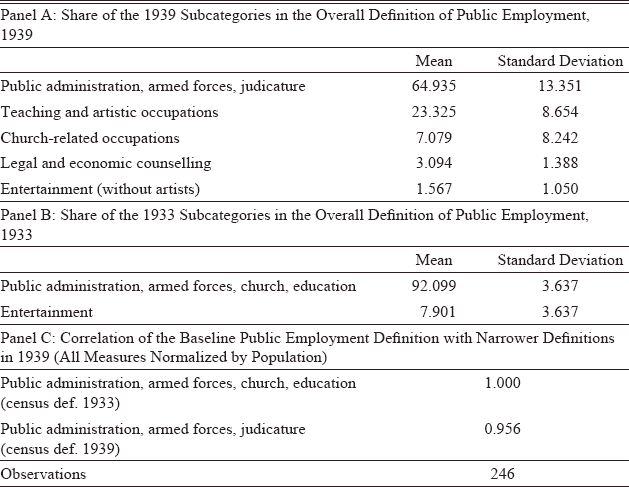
Although this wider definition introduces additional noise into my outcome variable, Table 1 provides evidence that public administration proper is the key component and driver of the measure that I am using. In panel A, I use the narrower 1939 employment categories to decompose my aggregated 1939 measure. As can be seen, nearly two-thirds of the people working in public employment according to my wide definition worked in occupations belonging to public administration and the armed forces. Typical occupations in this category in 1939 include officers, non-commissioned officers, and long-serving privates (no conscripts) in the Wehrmacht, civil servants in various levels of public administration, and the police (see Online Appendix A). In panel B, I decompose my aggregated measure in 1933 into the two components that the 1933 census reports separately. Artists and entertainers are only a very small component.Footnote 10 Finally, and most importantly, panel C shows that the variation that my aggregate measure uses is similar to the variation in the narrower categories of public employment according to the 1933 and 1939 definitions: in 1939, my aggregated measure of public employment is highly correlated with the number of workers in the narrower 1939 census category of public administration, armed forces, and judicature (both numbers normalized by city population) and even more so with the somewhat broader 1933 category. Thus, while aggregating several census categories introduces noise, the resulting variable still seems to be driven to a very large extent by public administration proper.
ASSESSING OUTCOME VARIABLE

Source: Own calculation based on German occupational censuses of 1933 and 1939.
To address additional concerns, I will show that using only 1933 and 1939 and the narrower definition of public employment according to the 1933 census leads to similar results, as does using the number of civil servants (Beamte) across all sectors, which is available for 1933 and 1939. I will also show cross-sectional results for 1939 only, using the narrower categories of the 1939 census.
In my baseline results, I will use the data from 1925, 1933, and 1939 and thus the wider, but internally consistent public employment definition described earlier. My main outcome variable is the log of the number of public administration jobs. Because German cities experienced considerable population growth between 1925 and 1939, I examine the ratio of public administration jobs to total population and the ratio of public administration jobs to the labor force. While the latter measure is robust to population changes, it is subject to another type of criticism: public investment is likely to also have increased employment in other sectors (e.g., due to increased spending on construction or military equipment). In some cities, growth in these industries might have outpaced growth in public employment, leading to a decrease in the ratio of public employment out of the population or labor force, even though the city might still have been benefiting from increased public employment. Put differently, a relative increase in one of the two ratio measures might just mean that the rest of the city's economy was doing relatively poorly, thereby increasing the share of public sector jobs. However, this is not a concern for the natural logarithm specification, which measures absolute, rather than relative, increases in public employment. Both the absolute and the relative measures therefore have their respective advantages and disadvantages. In practice, both lead to similar results, as I show later.
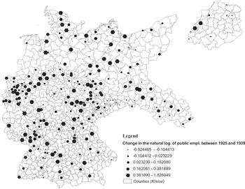
The advantage of using public sector employment is that most of the respective job categories are under the direct control of the central or local government (e.g., the number of officers and non-commissioned officers in the armed forces) and less constrained by the pre-existing regional industry, making them a more natural outcome measure that also has closer resemblance to the individual-level outcome measure employed by, for example, Hsieh, Miguel, Ortega, et al. (Reference Hsieh, Miguel and Ortega2011). Data on public employment is available for nearly 300 cities; in particular, it is available for all cities with more than 20,000 inhabitants and for some smaller ones that happened to be independent cities, not belonging to any other administrative district (Kreisfreie Städte). Figure 1 illustrates the geographical distribution of public employment growth over the sample period. Specifically, it maps quintiles of the difference in the natural logarithm of public employment between 1925 and 1939. As can be seen, increases in public employment are spread relatively evenly across the country, with perhaps a small concentration of stronger increases in Central Germany.
CHANGES IN PUBLIC EMPLOYMENT BETWEEN 1925 AND 1939

The main explanatory variable of interest is the NSDAP vote share in the election of March 1933. For this, I use the extensive database on social and electoral variables for Weimar Germany compiled by Jürgen Falter and Dirk Hänisch (Reference Falter and Hänisch.1990). This database also contains other socioeconomic variables that might be of interest when analyzing NSDAP vote shares. In particular, I include the Jewish share of a city's population in 1925 and the unemployment rate at the time of the census in 1933.Footnote 11 In addition to these socioeconomic variables, I control for longitude, latitude, an indicator for being in the Rhineland and an indicator for being the capital of a Nazi “Gau” (see later). These variables are included to control for potential geographic determinants of public, especially military employment.
According to Articles 42–44 of the Versailles Treaty, Germany was not allowed to maintain or construct fortifications or station troops on the left (Western) bank of the Rhine or within 50km of its right (Eastern) bank. In 1936, Hitler violated this stipulation by “reoccupying” the Rhineland with armed forces. If the Rhineland is also correlated with voting behavior, this could create a spurious correlation between public employment and vote shares. To avoid this concern, I control for a city lying in the “Rhineland” as defined by the Versailles Treaty. Similarly, the territorial reorganization of the former German states (Länder) into new units called Gaue might also have led to differential changes in public employment in the Gau capital cities. If these capital cities had also been more likely to vote for the Nazis, again a spurious correlation might arise. I therefore include an indicator for whether a city was a Gau capital in 1938 (Das Buch der deutschen Gaue 1938).
A potential problem is the question of whether a city in 1925 was the same city in 1933 and 1939, as many German cities underwent changes in their territory and population, acquiring smaller surrounding towns and villages, merging with other cities and the like. A prime example is Wilhelmshaven, which more than quadrupled its population between 1933 and 1939 with the acquisition of the neighboring city of Rüstringen. Similar mergers occurred in the Ruhr area in 1928–1930. In order to avoid problems due to these territorial restructurings, I excluded all cities which experienced a substantial enlargement in their population between 1910 and 1925, 1925 and 1933, or 1933 and 1939.Footnote 12
In addition, I use voting data from the 1912 Reichstag election, for which I have city-level data for all cities that had more than 10,000 inhabitants in 1910. These were obtained from the official election results, published by the Statistisches Reichsamt in 1913. Ultimately, I have a sample of 246 cities for the three census years 1925, 1933, and 1939. Because the 1933 census was administered on June 16, four and a half months after Hitler had become chancellor, but still before his large-scale rearmament programs had begun, I usually treat it as a pre-NSDAP year but will show later that my results are not driven by this.
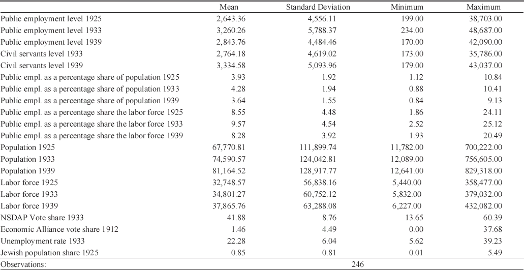
In Table 2, I provide summary statistics of the explanatory and explained variables. As can be seen, both the number and shares of public employees increased from 1925 to 1933, and then decreased again. The number of public employees is higher in 1939 than in 1925, whereas their shares of total population or labor force are lower. Given the large amount of public investment and the substantial increase of the German armed forces between 1933 and 1939, this might seem surprising. The most likely explanation is that public employment was driven up between 1925 and 1933 by general employment measures, used as a means of fighting unemployment even before the Nazis came to power. Hitler's predecessors von Papen and von Schleicher had already made credit and funding for public employment measures available (Golecki Reference Golecki, Erdmann, Mommsen and Vogel1986, pp. XXXIV–XL). Fritz Blaich (Reference Blaich1970) uses the example of Ludwigshafen to show how cities themselves tried to fight the economic crisis by employing otherwise unemployed workers in the construction of roads and sewerage systems. This pattern of a strong increase as a reaction to the economic crisis makes it even more difficult to uncover the causal effect of the NSDAP vote share using a standard ordinary least square (OLS) approach. Cities where more of these emergency projects were carried out could experience an increase in public employment between 1929 and 1933, followed by a decrease until 1939, when full employment had rendered these emergency measures obsolete. As an alternative measure of public employment, I also use the number of civil servants (Beamte) across all sectors. Data for this variable exists for 1933 and 1939, and this measure (which should measure more permanent jobs, but across a wider spectrum of sectors) shows a raw increase even between 1933 and 1939. The mean NSDAP vote share in my sample of cities is 41.8 percent, very close to the national average of 43.9 percent. The 1912 Economic Association was a much smaller party. Across my whole sample, it averaged 1.5 percent of all votes, but with a sizeable dispersion; in 191 cities it did not receive any votes, while four cities recorded EA vote shares greater than 20 percent.
SUMMARY STATISTICS

Source: Public employment and labor force data for all three years are from Statistisches Reichsamt (Reference Statistisches1927–1928, Reference Statistisches1935–1936, Reference Statistisches1942). Civil servants and population in 1939 are from Statistisches Reichsamt (Reference Statistisches1942). 1912 EA vote share data are from Statistisches Reichsamt (Reference Statistisches1913). All remaining data are based on Falter and Hänisch (Reference Falter and Hänisch.1990).
The “Economic Association” and Its Voters
It is unlikely that a simple OLS regression, even after controlling for city fixed effects and control variables, can uncover the causal effect of Nazi support on subsequent public employment. The main endogeneity concern in such a regression is the economic crisis in the years following 1929. For example, cities that were more adversely affected by the crisis might have been differentially prone to vote for the NSDAP in 1933 and they might also have been subsequently those with different public employment shares. The NSDAP vote share would then be correlated with the error term, and as a consequence, the estimate of β in such a regression will be inconsistent. Another problem could arise if public employees themselves are more or less likely to vote for the NSDAP, creating a reverse causality problem. Finally, Voigtländer and Voth (Reference Voigtländer and Voth2016) have shown that local highway construction caused increased support for the NSDAP government, suggesting an additional reverse causality problem: voting behavior affects public spending, but public spending (or expected public spending) also affects voting behavior.
In order to address these issues of potential endogeneity, I instrument the 1933 NSDAP vote share by the vote share of another party, the “Economic Association” (Wirtschaftliche Vereinigung, henceforth EA) in the 1912 election. The EA was an alliance of several smaller parties, most notably the “Christian-Social Party” (Christlich-Soziale Partei) and the “German-Social Party” (Deutschsoziale Partei). Most of these parties had conservative, nationalist platforms that denounced both socialism and capitalism and tried to attract middle-class voters particularly in Protestant and rural areas. In addition, both the “Christian-Social Party” and the “German-Social Party” were openly anti-Semitic (Gräfe Reference Bergmann and Benz2012; Bergmann Reference Bergmann and Benz2012). The constituent parties of the EA were not strong, and the alliance only obtained a few seats in the 1912 election. However, there are strong parallels between the voters that the EA tried to attract, and the voters that in 1933 voted for the NSDAP.
The NSDAP had started out using anti-capitalist and socialist rhetoric, catering to the preferences of blue-collar voters. It markedly changed its approach as a result of its disappointing results in 1928. After 1928, the party focused more on rural areas and presented itself less as a radical force against capitalism, but rather as an ultra-nationalist, conservative party that advocated law and order and the fight against the Treaty of Versailles. The aim was to attract more middle-class voters who heretofore had been repulsed by the party's more proletarian agenda (Stachura Reference Stachura1978). This transformation was successful; by 1933, the NSDAP had become, in the words of Jürgen Falter (Reference Anderson and Tollison1991, p. 372), “a people's party with a middle-class belly” (eine Volkspartei mit Mittelstandsbauch), in which the middle classes were the largest fraction. Thus, after 1928, the NSDAP presented itself more as an ultra-nationalist party for the middle-class, with a particular focus on rural and Protestant voters, trying to attract the very voters that the EA, before WWI, had tried to attract, as well as sharing its antisemitism.Footnote 13 Because of this, the vote share of the EA in the 1912 election and the NSDAP vote shares after 1928 are significantly positively related (this is also shown more formally in the first-stage results later), so the former can be used as an instrument for the latter.
The basic idea of this instrument is to use variation in NSDAP vote shares that is not due to the economic crisis post 1929, but due to persistent political attitudes of the local population such as extreme nationalism or antisemitism.Footnote 14 In order to be a valid instrument, the 1912 EA share has to satisfy the exclusion restriction. In particular, the identifying assumption of this strategy is that the 1912 EA share does not have an effect on public employment outcomes later on, other than through affecting support for the NSDAP. Several aspects make the 1912 EA vote share attractive in this respect. Firstly, dating from more than 20 years prior to the 1933 election, use of the 1912 EA share should not be susceptible to reverse causation problems either from public spending in the Weimar era, expected public spending by a potential NSDAP government, or the voting behavior of public employees. Secondly, using a vote result prior to the economic crisis starting in 1929 allows me to purge the 1933 vote shares of any factors from this crisis.
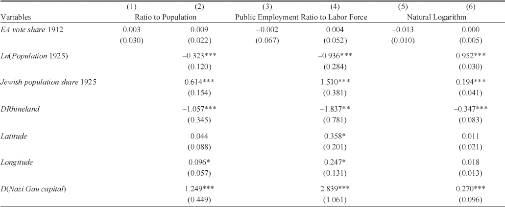
One remaining concern, however, is that there might still be unobserved factors that are correlated both with the 1912 EA share and with the 1933 NSDAP share and that might also be relevant for the evolution of public employment over time. Cities with a high EA share might be fundamentally different from those with low or no EA votes, and these differences might also affect public employment patterns. The absence of such differences cannot be tested or proved in a formal sense. However, I can examine whether the instrument is correlated with the level and evolution of relevant variables before 1933. In Table 3, I run a cross-sectional regression for 1925, relating the three public employment outcomes (the ratio of public employment to either the population or the labor force, and the natural logarithm of public employment) to the 1912 EA vote share. Odd numbered columns (1, 3, 5) show simple bivariate correlations, even numbered columns (2, 4, 6) include controls. Since I cannot include fixed effects in the cross-sectional regressions, I include the natural logarithm of a city's population as an additional control to make sure I compare cities of similar size. I omit the 1933 unemployment rate from these 1925 regressions. There is clearly no relationship between public employment in 1925 and the 1912 EA vote share. Regardless of the inclusion or exclusion of controls, the estimates are statistically insignificant and of small magnitudes. For example, according to the specification with controls, increasing the 1912 EA vote share by one full standard deviation would decrease the 1925 public administration jobs to population ratio by only 2 percent of a standard deviation.
CHECK FOR DIFFERENT LEVELS IN PUBLIC EMPLOYMENT IN 1925

* = Significant at p<0.1.
** = Significant at p<0.05.
*** = Significant at p<0.01.
Notes: Cross-sectional results for 1925 with 246 cities. Controls are the natural logarithm of city population, longitude, latitude, an indicator for the Rhineland, an indicator for being a Gau capital, and the Jewish population share in 1925. Robust standard errors in parentheses.
Sources: 1912 EA vote share from Statistisches Reichsamt (Reference Statistisches1913), public employment jobs and labor force from Statistisches Reichsamt (Reference Statistisches1927–1928, Reference Statistisches1935–1936), latitude and longitude from online geocoding tools, Rhineland according to the definition of the Versailles treaty, Nazi Gau capitals from Das Buch der Deutschen Gaue (Reference Ritschl1938), remaining data from Falter and Hänisch (Reference Falter and Hänisch.1990).
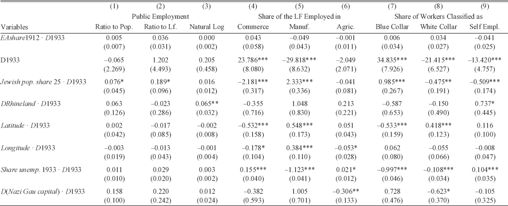
The absence of a correlation between my instrument and the level of public employment in 1925 is reassuring, but the identifying assumption of my strategy is not that the 1912 EA vote share is uncorrelated with the counterfactual level of public employment, but with its counterfactual changes. To assess this, in columns 1–3 of Table 4, I show the results of a “placebo test,” examining whether cities with different 1912 EA vote shares experienced different evolutions of public employment between 1925 and 1933. Specifically, I regress my three outcomes on the interaction between the 1912 EA share and an indicator for the year 1933, an indicator for the year 1933, city fixed effects, and my control variables, each of which is interacted with an indicator for the year 1933. The results from this exercise are encouraging. The 1912 EA vote share is never significantly associated with the development of public employment between 1925 and 1933, and the point estimates are small. For example, increasing the 1912 EA vote share by one standard deviation is associated with an increase in administration jobs as a ratio to total population of less than 1 percent of a standard deviation of the 1925 administration job ratio. Even more encouraging, in columns 4–6, when I examine whether the 1912 EA share is correlated with the evolution of a city's economy as measured by the employment shares of three broadly defined sectors, I again do not find any relationship. Between 1925 and 1933, cities with high or low 1912 EA vote shares do not experience different evolutions of employment in either agriculture, manufacturing, or commerce. Finally, in columns 7–9, I look at the occupational class composition of a city's economy, measured by the respective shares of blue-collar employees, white-collar employees, and self-employed. Again, there is no relationship between voting for the Economic Association and changes in a city's occupational class structure.Footnote 15
CHECK FOR DIFFERENT TRENDS IN PUBLIC EMPLOYMENT AND OTHER SECTORS BEFORE 1933

* = Significant at p<0.1.
** = Significant at p<0.05.
*** = Significant at p<0.01.
Notes: Panel data results for 1925 and 1933 with 246 cities and 492 observations. Robust standard errors, clustered at the city level, in parentheses. All regressions control for city fixed effects, an indicator for 1933 as well as interactions of an indicator for 1933 with an indicator for being a Gau capital, the Jewish population in 1925, the unemployment rate in 1933, longitude, latitude, and an indicator for being in the Rhineland.
Sources: 1912 EA vote share from Statistisches Reichsamt (Reference Statistisches1913), public employment jobs and labor force from Statistisches Reichsamt (Reference Statistisches1927–1928, Reference Statistisches1935–1936), latitude and longitude from online geocoding tools, Rhineland according to the definition of the Versailles treaty, Nazi Gau capitals from Das Buch der Deutschen Gaue (1938), remaining data from Falter and Hänisch (Reference Falter and Hänisch.1990).
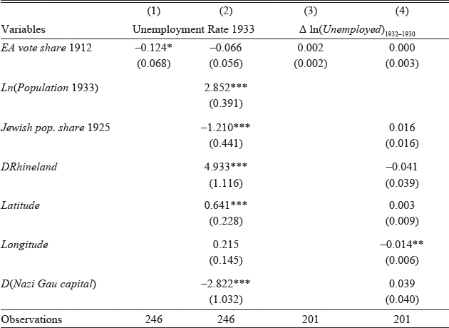
An important question is whether cities with different 1912 EA vote shares were affected differentially by the economic crisis after 1929. I provide a coarse assessment of this in Table 5, where I correlate unemployment during the crisis with voting for the EA in 1912. A slight negative bivariate correlation is present between the unemployment rate in 1933 and the 1912 EA vote share, but this is not robust to the inclusion of controls. In addition, when looking at changes in unemployment by regressing the difference in the logs of unemployment in 1932 and 1930 on the 1912 vote share, I again do not detect any sizable or statistically significant relationship.
RELATIONSHIP BETWEEN THE INSTRUMENT AND THE ECONOMIC CRISIS

* = Significant at p<0.1.
** = Significant at p<0.05.
*** = Significant at p<0.01.
Notes: Cross-sectional results for 1925. Controls are longitude, latitude, an indicator for the Rhineland, an indicator for being a Gau capital, and the Jewish population share in 1925. Column 2 also controls for the natural logarithm of city population. Robust standard errors in parentheses.
Sources: 1912 EA vote share from Statistisches Reichsamt (Reference Statistisches1913), latitude and longitude from online geocoding tools, Rhineland according to the definition of the Versailles treaty, Nazi Gau capitals from Das Buch der Deutschen Gaue (1938), remaining data from Falter and Hänisch (Reference Falter and Hänisch.1990).
These results strengthen the instrument's case for exogeneity: the 1912 EA share is not correlated with the level of or evolution of public employment between 1925 and 1933. It is also not associated with changes in the city's sectoral or occupational class structure. Finally, there is also no evidence that cities with high EA vote shares experienced different evolutions of unemployment during the economic crisis in the early 1930's. It is still possible that cities with high and low EA votes differed along other dimensions, but the previous results seem to indicate that such differences, if present, were not very consequential in economic terms.
Based on this, I employ a standard two-stage least square estimation procedure. The basic model of interest is:

where y it represents the outcome, that is, either the natural logarithm of public employment or the ratio of public employment to population, or the labor force in city i and year t, where t can be 1925, 1933, or 1939. NSDAPshare33i denotes the NSDAP vote share in the 1933 election in city i and D1939t is a dummy which is 1 for the year 1939. The city fixed effects, c i, will account for constant effects of time invariant city characteristics such as being a historical regional capital. X is a vector of time-invariant city-level controls, discussed in the previous section. To address the endogeneity problem arising from the likely correlation between the 1933 NSDAP vote share and the economic crisis, the variable of interest in equation 1 will be replaced by its prediction based on the same controls and the 1912 EA share:

These predicted values will then be used as regressors of interest in the second stage:

RESULTS
Baseline Estimates
Table 6 presents the results of simple OLS estimations from equation 1. As discussed in the previous section, these regressions are based on the strong assumption that the 1933 NSDAP vote share is exogenous, that is, uncorrelated with the error term, which is unlikely given the 1929 economic crisis. An extensive body of literature has analyzed the reasons for the NSDAP's rapid electoral successes, which socioeconomic groups were more likely to vote for the National Socialists and why they did so (see, among others, Frey and Weck Reference Frey and Weck1981; Falter, Link, Lohmöller, et al. Reference Falter, Link and Lohmöller1983, Reference Falter, Link and Lohmöller.1985; Falter Reference Falter1991; van Riel and Schram Reference van Riel and Schram1993; Stögbauer Reference Stögbauer2001; King, Rosen, Tanner, et al. Reference King, Rosen and Tanner2008; Adena, Enikolopov, Petrova, et al. Reference Adena, Enikolopov and Petrova2015; Koenig Reference Koenig2015; Satyanath, Voigtländer, and Voth Reference Satyanath, Voigtländer and Voth2017; Spenkuch and Tillman forthcoming;). Although some disagreement about certain issues still exists, there is a clear consensus that the economic crisis that affected Germany in the early 1930s was a prime driver of National Socialist vote shares. If cities that were affected more by the crisis were differentially likely to vote for the NSDAP in 1933, the OLS estimates will be biased. The sign of the bias is unclear a priori: if cities more affected by the crisis were more industrialized and therefore more strongly connected to the communist parties, and public employment increased in these cities as a response to the crisis, the resulting OLS estimate could be biased downwards. A similar negative bias could arise if public servants were more likely to vote for the NSDAP and cities with more public employment experienced slower growth in public employment (e.g., since they were less affected by the crisis and thus did not need large-scale investment programs, or at least only smaller ones). On the other hand, if cities that were affected more by the crisis turned towards the Nazis, it is easily conceivable that an upward bias might arise.Footnote 16 With this in mind, the estimates of β in Table 6 are negative, but not large and not significantly different from zero. Taken at face value, this would mean that a city's NSDAP vote share in 1933 had no or a slightly negative effect on the city's public employment share in 1939. This could mean that if anything, instead of “favoring” loyal cities, the new government tried to “buy support” from more resistant cities, for example, in an attempt to stabilize its power in the early days of the regime. However, these OLS estimates should be viewed with caution, and I turn next to the instrumental variable (IV) estimates discussed earlier. By using an instrumental variable that significantly predates the 1929–1932 economic crisis, this approach avoids any correlation between the NSDAP vote shares and the intensity of the crisis.
OLS ESTIMATES

* = Significant at p<0.1.
** = Significant at p<0.05.
*** = Significant at p<0.01.
Notes: Panel data results for 1925, 1933, and 1939, 246 cities and 738 observations. Robust standard errors, clustered at the city level, in parentheses. All regressions control for city
fixed effects, an indicator for 1939 as well as interactions of an indicator for 1939 with an indicator for being a Gau capital, the Jewish population in 1925, the unemployment rate in 1933, longitude, latitude, and an indicator for being in the Rhineland.
Sources: 1912 EA vote share from Statistisches Reichsamt (Reference Statistisches1913), public employment jobs and labor force from Statistisches Reichsamt (Reference Statistisches1927–1928, Reference Statistisches1935–1936, Reference Statistisches1942), Reference Statistisches1939 population from Statistisches Reichsamt (Reference Statistisches1942), latitude and longitude from online geocoding tools, Rhineland according to the definition of the Versailles treaty, Nazi Gau capitals from Das Buch der Deutschen Gaue (1938), remaining data from Falter and Hänisch (Reference Falter and Hänisch.1990).
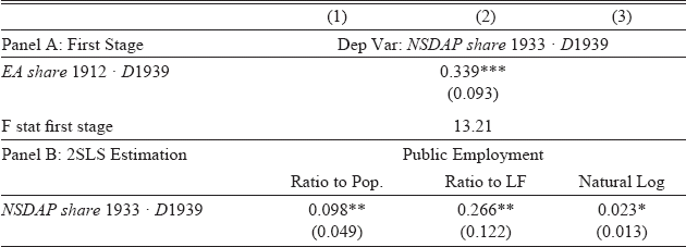
The 2SLS estimates based on the 1912 vote share for the “Economic Association” as instrumental variable for the 1933 NSDAP vote share are presented in Table 7. As can be seen from the first stage result, the 1912 EA vote share and the 1933 NSDAP vote share are indeed strongly and, as one would expect, positively related. The first-stage results indicate that a 1 percentage point increase in the 1912 EA vote share increases the 1933 NSDAP vote share by around 0.35 percentage points. Thus, the translation between 1912 EA voters and 1933 NSDAP voters is not one-to-one, which is not surprising, given that some members of the Economic Alliance joined other parties after 1918, in particular the German National People's Party, Hitler's coalition partner from January 1933 (Bergmann Reference Bergmann and Benz2012).
IV ESTIMATES

* = Significant at p<0.1.
** = Significant at p<0.05.
*** = Significant at p<0.01.
Notes: Panel data results for 1925, 1933, and 1939, 246 cities and 738 observations. Robust standard errors, clustered at the city level, in parentheses. All regressions control for city fixed effects, an indicator for 1939 as well as interactions of an indicator for 1939 with an indicator for being a Gau capital, the Jewish population in 1925, the unemployment rate in 1933, longitude, latitude, and an indicator for being in the Rhineland.
Sources: See note to Table 6.
In panel B, I find that an increase in the 1933 NSDAP vote share of 1 percentage point would increase the number of public sector jobs by around 2.3 percent, which is a quite substantial increase. When looking at public employment as a share of population, the results indicate that a 1 percentage point increase in the 1933 NSDAP vote share is associated with a 0.1 percentage point increase in the ratio of public employment to total population. Put differently, an increase of one standard deviation in the 1933 vote share leads to an increase of around 45 percent of a standard deviation in terms of the 1925 public employment share. The results for public employment as a share of the labor force are similar in magnitude.Footnote 17 All these results are relative results. They show that cities with greater NSDAP vote shares experienced a relative increase in public employment compared to cities with lower Nazi support. As the summary statistics presented earlier show, both the number of public employment jobs and its shares are lower in 1939 than in 1933. In this sense, my results show that public employment fell less for cities with greater NSDAP support.
The results from Table 7 show that high 1933 NSDAP vote shares led to a subsequent relative increase in public sector jobs, both in absolute numbers and in ratios of the population. This pattern thus is not consistent with the Nazi government buying support from opposing cities, but rather rewarding its strongholds via public employment.
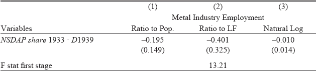
In Table 8, I provide further evidence that my results are based on government discrimination, rather than other economic forces. Here, I repeat the analysis, but this time using the metal industry, a sector that contracted during the 1929 crisis and expanded during the pre-war build-up, but was not under direct government control. I would not expect to find an effect here.Footnote 18 The estimates are all not significantly different from zero. In the case of the ratios of administration employment to the labor force and to the labor force, the point estimates are relatively sizable, but very imprecisely estimated, whereas for the natural logarithm also the point estimate would indicate a very limited negative effect of 1 percent.
METAL INDUSTRY

* = Significant at p<0.1.
** = Significant at p<0.05.
*** = Significant at p<0.01.
Notes: Panel data results for 1925, 1933, and 1939, 246 cities and 738 observations. Robust standard errors, clustered at the city level, in parentheses. All regressions control for city
fixed effects, an indicator for 1939 as well as interactions of an indicator for 1939 with an indicator for being a Gau capital, the Jewish population in 1925, the unemployment rate in 1933, longitude, latitude, and an indicator for being in the Rhineland.
Sources: Metal industry employment jobs and labor force from Statistisches Reichsamt (Reference Statistisches1927–1928, Reference Statistisches1935–1936, Reference Statistisches1942). All other variables see notes to Table 6.
One caveat is that part of the increased importance of public sector jobs could be due to supply factors rather than increased demand. In cities leaning more towards the Nazis, more people might have decided to work in the public administration or join the armed forces, whereas Nazi opponents might have voluntarily left their jobs. While such differential supply-side behavior is possible, the local or regional governments still would have had to create the necessary vacancies.
Robustness
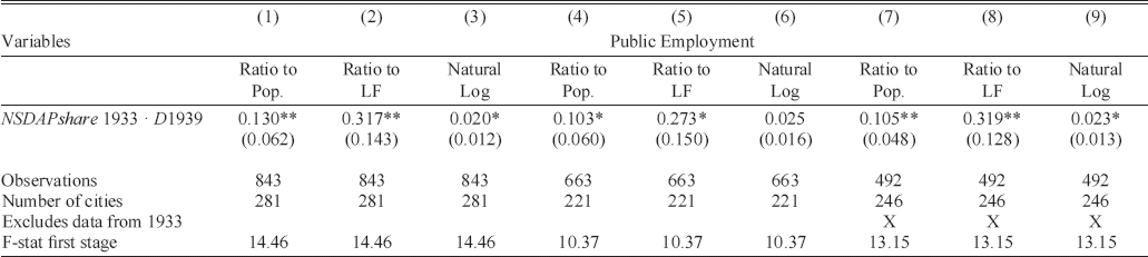
I now address several potential concerns relating to the findings from the IV regressions. As discussed earlier, there were several city mergers and restructurings between 1925 and 1933. While I tried to exclude all cities whose population growth was mostly driven by territorial enlargement, a certain arbitrary element remains. When are territorial changes so important that a city is no longer comparable over time? In columns 1–6 of Table 9, I repeat the analysis of Table 7 for two different and somewhat “extreme” samples. In columns 1–3, I do not drop any cities; in columns 4–6, I exclude all cities whose growth between either 1910 and 1925, 1925 and 1933, or 1933 and 1939 exceeded the respective mean by more than one respective standard deviation. For convenience, the first stage results are omitted and only the respective F statistic is displayed. Compared to the main results in Table 7, standard errors increase both when including more cities (columns 1–3) and when including fewer (columns 4–6). In the latter case, the point estimates are very similar to the main specification, whereas not dropping any cities if anything seems to lead to slightly larger point estimates. Overall, however, the qualitative conclusions from before do not change, lending support to my hypothesis.
ROBUSTNESS: CITY SIZE AND DROPPING 1933

* = Significant at p<0.1.
** = Significant at p<0.05.
*** = Significant at p<0.01.
Notes: Panel data results for 1925, 1933, and 1939. Robust standard errors, clustered at the city level, in parentheses. All regressions control for city fixed effects, an indicator for 1939 as well as interactions of an indicator for 1939 with an indicator for being a Gau capital, the Jewish population in 1925, the unemployment rate in 1933, longitude, latitude, and an indicator for being in the Rhineland. Columns 1–3 do not drop any cities that underwent size changes during the period of observation; columns 4–6 exclude all cities whose growth between either 1910 and 1925, 1925, and 1933, or 1933 and 1939 exceeded the respective mean by more than one respective standard deviation. Columns 7–9 keep the standard set of cities, but exclude data from 1933.
Sources: See note to Table 6.
So far, I have treated 1939 as the only year after the NSDAP rise to power, taking 1925 and 1933 to be pre-treatment years. I do this because the first large-scale public investment program by the National Socialists, the Rheinhardt program, started in June 1933, a few days before the 1933 census data were collected, and the expansion of the armed forces occurred even later. Against this, one can argue that the National Socialists came to power in January 1933 and already had a parliamentary majority after March 1933. As shown by Ferguson and Voth (Reference Ferguson and Voth2008), shareholders immediately reacted to this change in power, and so therefore might have other economic variables. Moreover, the Nazis' prosecution of their political enemies began after the Reichstag Fire in February 1933, which might also have had implications for public employment. Similarly, the “law for the restoration of the professional civil service” had already been passed in April 1933. Hence, treating 1933 as a pre-treatment year might be problematic, though if anything, it would most likely bias my estimates towards 0.
In columns 7–9 of Table 9, I examine the effect of dropping the potentially confounded year 1933, only comparing 1925, a clear pre-treatment year, to 1939, a clear post-treatment year. The results are again very similar to the baseline results and if anything slightly larger, which would be in line with the 1933 numbers already being slightly contaminated by the Nazi rise to power. However, any such contamination appears to be very limited.
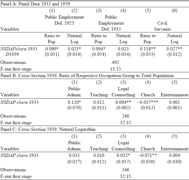
Another potential problem is the wide definition of public employment that I use throughout the analysis. As discussed earlier, creating a consistent measure for 1925, 1933, and 1939 requires aggregating several occupations, some of which are clearly not part of “public employment.” This will increase the noise in my outcome variable and thus impair the precision of my estimates, but if these other jobs also react to the Nazi rise to power, it could introduce biases. In Table 10, I examine the robustness of my results with regards to different outcome variables. Such variables do not exist for 1925. In panel A, I focus on variables that exist for both 1933 and 1939, panels B and C show results for variables that are only available for 1939. In columns 1 and 2 of panel A, I show results for my baseline outcome for 1933 and 1939. For brevity, I focus on the natural logarithm of public employment and the ratio of public employment to population as outcome variables, omitting the ratio of public employment to the labor force which is very highly correlated with the ratio out of population. The results when using 1933 and 1939 are very similar to the main results in Table 7, which is further evidence that despite the census in 1933 occurring after the election, 1933 is still a valid pre-treatment year. In columns 3 and 4 then, I use a more narrow public employment definition that omits the cinema, theatre, and other entertainment occupations. The results are very similar to those in columns 1 and 2. In columns 5 and 6, I employ a different outcome variable. Instead of trying to get at the public administration sector, I use the occupational class of civil servants (Beamte) across all sectors.Footnote 19 Again, results are very similar: increasing the 1933 NSDAP vote share by 1 percentage point would lead to an increase in the number of civil servants by 2.7 percent, very much in line with the 2.3 percent in column 2 of this table and column 3 in Table 7.
ROBUSTNESS: OUTCOME MEASURE

* = Significant at p<0.1.
** = Significant at p<0.05.
*** = Significant at p<0.01.
Notes: Results for 246 cities. Standard errors (panel A: clustered at the city level, panels B and C: robust) in parentheses. Panel A regressions control for city fixed effects, an indicator for 1939 as well as interactions of an indicator for 1939 with an indicator for being a Gau capital, the Jewish population in 1925, the unemployment rate in 1933, longitude, latitude, and an indicator for being in the Rhineland. Panel B regressions control for the natural logarithm of city population, longitude, latitude, an indicator for the Rhineland, an indicator for being a Gau capital, the unemployment rate in 1933, and the Jewish population share in 1925.
Sources: See notes to Table 6.
An even narrower definition of public employment is possible when using data from 1939 only. In panels B and C of Table 10, I show results from cross-sectional regressions for the five narrow employment categories that together form my employment definition that is consistent across the three censuses. These regressions cannot control for fixed effects and therefore rely on stronger identifying assumptions. To at least partly remedy this, I include the natural logarithm of a city's population as additional control. In panel B, I show the respective ratio of each of the five categories to total population. The overall increase in the ratio of public employment to population is driven mostly by public administration and the armed forces. Legal and economic counselling and teaching occupations show at most a very slight increase. Entertainment does not respond at all, whereas church-related occupations even decrease. Panel C, which uses the natural logarithm, by and large confirms the previous findings. However, the estimate for public administration becomes relatively imprecise and loses statistical significance. Still, the point estimate of a 3.1 percent is very similar and if anything slightly larger than previous results. Overall, public administration and the armed forces appear to be the prime drivers of my measure of public employment. Taken together, the results in Table 10 show that while the aggregation of several occupational classes is undesirable from a conceptual point of view, it seems to have little implications for the sign or magnitude of my results.
CONCLUSION
Between 1928 and 1933, the NSDAP developed from a small and unimportant party in Weimar Germany into the strongest party in the German parliament, making its leader Adolf Hitler the head of the German government by January 1933 and gaining a parliamentary majority by March of the same year. Hitler used this power not only to concentrate all political competences among his followers, but also to enact large public investment and rearmament programs and to overhaul the civil service. In this article, I document evidence that the public employment policies during the early Nazi era were not ideologically color blind. Using a city's 1912 vote share of the Economic Alliance, a small party in Imperial Germany that catered to similar voters as the late NSDAP, as an instrumental variable for the 1933 NSDAP vote share, I find that the latter had a positive and significant effect on subsequent public employment at the city level. A 1 percentage point increase in the 1933 vote share caused the number of public employment jobs to grow by around 2.5 percent, a finding which is not driven by cities undergoing territorial changes or by the inclusion or exclusion of the potentially already contaminated census year of 1933, and is also robust to using different definitions of public employment as outcome variables. This relative increase at the local level is happening as the German economy recovers and the number of public employees declines nationwide. My findings show that this decline was less pronounced in cities that had voted more for the NSDAP.
The results of this study shed additional light on the ability of governments to use economic policy as a means to reward and protect their voters and supporters, and/or to punish their political adversaries. It adds to a growing body of literature that has documented such behavior on a firm-level and, to a certain extent, also for individuals. Of course, some cautionary remarks apply. In particular, Germany's Nazi government had stronger powers than many modern democratic governments. Being freed of the constraints usually posed by a parliamentary opposition, judicial review by courts, and a free press, it seems reasonable to assume that the National Socialists' ability to reward a city's loyalty was substantially larger than in countries with a stronger opposition.
Anecdotal evidence suggests that one important mechanism behind my finding is the preferred allocation of public sector jobs to loyal party stalwarts. This reflected a propagandistic cult around the hardships of the party's “old guard,” but also the NSDAP's internal structure, which was marked by cliques, where followers expected their superiors to reward them in return for their loyalty. Several questions remain in this respect for future research: can this behavior also be documented at the individual level? Were there other channels through which public employment was targeted towards cities favoring the Nazis? Are there any long-term effects of the increased public employment in the 1930s? Did the economic reward for these cities survive WWII and persist longer than the Nazi government, or did it disappear when the favored party members lost office? And, in a broader context, what are the welfare implications of such favoring behavior? In these respects, there is substantial scope for further research.
Appendix
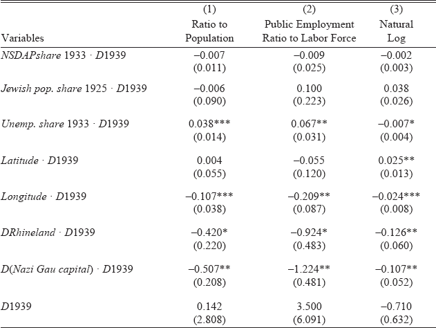
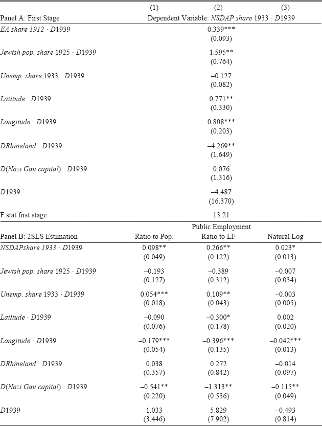
In my empirical strategy, I use several control variables detailed in the data section. Control variables are not of interest per se for my study. Moreover, in the absence of a credible identification strategy for them, their regression coefficients identify mere conditional correlations without a causal interpretation. Because of this, I have omitted them from the main regression tables. In Appendix Table 1 however, I show the basic fixed-effects regression results from Table 6, including the coefficients for all control variables. Appendix Table 2 does the same for the baseline IV estimates of Table 7.
OLS ESTIMATES

2SLS ESTIMATES

Conditional on all the other included variables, latitude, and the Jewish population share in 1925 do not appear to be correlated with public employment. Cities in the East experienced a relative decrease of public employment, while the dummy for the Rhineland is actually negative. Given the military reoccupation of the Rhineland after 1935, this is surprising, but on the other hand, the Rhineland and longitude are strongly negatively correlated, so part of this effect could potentially be captured by the longitude coefficient already. Cities with a greater unemployment rate in 1933 experience relative increases in public employment jobs in the ratio specifications (columns 1 and 2), but not in the log specification, which indicates that such cities experienced a relative population decline. Interestingly, NSDAP Gau capitals experienced declines in public employment. One explanation is that most Gau capitals were already regional or state capitals before the Nazis had come to power and thus already had sizeable public employment shares before, such that they on average experienced less growth.
Panel A of Appendix Table 2 shows the correlations of the control variables with the 1933 NSDAP vote share. The Jewish population share is positively correlated with voting for the Nazis, as is being in the East and North. Being in the Rhineland has a strong negative effect on the 1933 NSDAP vote share, which is not surprising given the region's Catholicism and the findings of Spenkuch and Tillman (forthcoming). Gau capitals and the 1933 unemployment rate, on the other hand, are not found to have statistically significant effects on voting for the Nazis. The negative point estimate for the unemployment rate is in line with Falter, Link, Lohmöller, et al. Reference Falter, Link and Lohmöller.1985, who find a negative correlation between the unemployment rate and the 1933 NSDAP vote share in a sample of precincts. Turning to the IV estimates in panel B, most of the estimates are similar to those in Appendix Table 1: latitude turns slightly negative, while the effect of the unemployment rate is again apparently due to differential population changes and thus absent in the logarithmic specification. Cities in the West still are found to have experienced growth in the public sector, whereas Gau capital cities are negatively associated with public employment growth. The one major change of the IV controls relative to the OLS controls is that the Rhineland coefficients are now considerably larger in value, sometimes even positive, but generally insignificant. Again, it seems that the public employment effect of being in the Rhineland is to a large extent already captured by the longitude effect.