INTRODUCTION
Since 1961, the world's population has grown by 126% (FAO 2014). To keep pace with increasing food demand resulting from population growth and rising per capita income, the Food and Agriculture Organization of the United Nations (FAO) has stated that to meet food security demands in 2050, agricultural production must increase by an estimated 60–100% above 2005 production levels (FAO 2015). As household income increases, people tend to consume more meat, which requires more resources and may have greater impact on the environment (McIntyre et al. Reference McIntyre, Herren, Wakhungu and Watson2009; Eshel et al. Reference Eshel, Shepon, Makov and Milo2014). Furthermore, as urban areas continue to expand, usually at the expense of high-value agricultural lands, pressure on producers to intensify production and to expand into lower value areas increases (McIntyre et al. Reference McIntyre, Herren, Wakhungu and Watson2009). Intensification of production has environmental consequences, such as greater contribution to climate change through greenhouse gas (GHG) emissions, increased risk of nitrogen (N) contamination of waterways, and deforestation (Bruinsma Reference Bruinsma2003; McIntyre et al. Reference McIntyre, Herren, Wakhungu and Watson2009; Dijkstra et al. Reference Dijkstra, France, Ellis, Strathe, Kebreab, Bannink and Kebreab2013). As global demand for beef increases, GHG, particularly methane (CH4) emissions, are expected to increase (Thornton Reference Thornton2010). Methane emissions contribute a proportion of 0·15 of world GHG emissions (FAO 2013), but the relative contributions vary among different regions of the world. Agriculture contributes the most towards world non-carbon dioxide (CO2) GHG emissions, accounting for 0·54 of world non-CO2 emissions in 2005, of which enteric CH4 comprises 0·33 of total agricultural emissions, or 0·18 of total non-CO2 emissions (US EPA 2012). Enteric CH4 emissions are expected to increase as global livestock populations increase, with the US EPA estimating a 22% global increase in CH4 emissions due to enteric fermentation from 2005 to 2030 (US EPA 2012).
To mitigate GHG emissions effectively, the processes involved in the production of emissions and production efficiency must be understood. Mechanistic models represent biological systems based on their components and seek to integrate processes at a lower level, such as organs, to predict at a higher level, such as the whole animal. AusBeef, a dynamic, mechanistic model of beef cattle production designed to optimize feedlot rations, was founded on the digestive and metabolic processes of the earlier MOLLY dairy cow research model (Baldwin et al. Reference Baldwin, France and Gill1987a , Reference Baldwin, Thornley and Beever b , Reference Baldwin, France, Beever, Gill and Thornley c ; Baldwin Reference Baldwin, France and Gill1995). Nagorcka et al. (Reference Nagorcka, Gordon, Dynes, McNamara, France and Beever2000), Nagorcka & Zurcher (Reference Nagorcka and Zurcher2002) and Nagorcka (Reference Nagorcka2004a , Reference Nagorcka b ) modified MOLLY to develop AusBeef, a feedlot-optimized model with modified parameter values as well as new additions to the model framework, such as an expanded set of microbial pools and different classes of feed particle size. Additional improvements were made based on ruminant studies by Dijkstra (Reference Dijkstra1993, Reference Dijkstra1994) and Dijkstra et al. (Reference Dijkstra, Neal, Beever and France1992, Reference Dijkstra, Gerrits, Bannink, France, McNamara, France and Beever2000). AusBeef integrates rumen microbial processes, as well as a voluntary feed intake mechanism, to predict not only animal performance and carcass characteristics, but also CH4 emissions.
The objectives of the present study were to: (1) describe the structure of AusBeef; (2) evaluate it against an independent data set; and (3) compare the accuracy and precision of predictions of daily methane production (DMP, g/day), gross energy intake (GEI, MJ/day) and methane yield (MY, MJ CH4/MJ GEI) by AusBeef with those from (a) the empirical National Academies of Sciences, Engineering and Medicine (NASEM 2016) beef production model and (b) the mechanistic L2 solution level of the Ruminant Nutrition System (RNS) model (Tedeschi & Fox Reference Tedeschi and Fox2016).
MATERIALS AND METHODS
General description of AusBeef
AusBeef is a dynamic, deterministic, mechanistic model that was developed for beef production and uses parameters derived for beef cattle (Nagorcka et al. Reference Nagorcka, Gordon, Dynes, McNamara, France and Beever2000; Nagorcka & Zurcher Reference Nagorcka and Zurcher2002; Nagorcka Reference Nagorcka2004a , Reference Nagorcka b ). AusBeef is a descendant of the MOLLY model of dairy cow production and uses its underlying architecture for the body growth and lower gut sub-models (Baldwin et al. Reference Baldwin, France and Gill1987a , Reference Baldwin, Thornley and Beever b , Reference Baldwin, France, Beever, Gill and Thornley c ; Baldwin Reference Baldwin1995). AusBeef was written in VISSIM (PTV 2004) and the user interface was constructed in Delphi with C++ code generated from VISSIM. The AusBeef model is integrated on a time step of 0·001 day (1·44 min). The model is an integration of four sub-models: rumen, body growth, lower gut and voluntary feed intake, each of which contains sub-modules that mechanistically represent physiological processes (Appendix 1; Hegarty Reference Hegarty2016). The AusBeef model can be integrated with the AusFarm biophysical whole-farm systems model (Herrmann Reference Herrmann2013) that is coupled with an animal growth model (Freer et al. Reference Freer, Moore and Donnelly1997; http://www.grazplan.csiro.au/?q=node/3). All parameter values and Michaelis–Menten equations of the sub-models within the AusBeef module can be accessed through a common modelling protocol (Moore et al. Reference Moore, Holzworth, Herrmann, Huth, Keating and Robertson2005) ‘a modular framework that enables sub-components of simulation models to be interchanged between different modelling software’.
In the present study, discussion is limited to the rumen sub-model, as the body growth and lower gut sub-models depend on outputs from the rumen sub-model. AusBeef inputs include: age, sex, breed, body condition score, initial average weight of animals in the herd, feed composition and feed management strategies. Feed characteristics are drawn from an internal database or specified by the user, which, combined with user-supplied costs and market price data, are used to simulate the growth and economics of beef cattle production.
Microbial groups
AusBeef represents four microbial pools including three bacterial pools: amylolytic bacteria (Ba), cellulolytic bacteria (Bc) and lactate-utilizing bacteria (Blc), and protozoa (Po). Amylolytic storage polysaccharides and protozoal storage polysaccharides are also represented as substrate pools associated with their respective microbial groups. Each microbial group has distinct coefficients for representing digestion and fermentation, and growth for all microbial groups is represented by Michaelis–Menten kinetics (Hegarty Reference Hegarty2016; Appendix 1). An important feature is the inclusion of lactate fermentation in the AusBeef rumen model. Lactate is produced in the rumen, and is then utilized and fermented to volatile fatty acids (VFA) by Blc. The balance between production and utilization usually keeps the concentration of lactate in the rumen low (Owens et al. Reference Owens, Secrist, Hill and Gill1998). However, in animals fed large quantities of rapidly degradable starch or soluble sugars, as in feedlots, or animals fed high-concentrate diets multiple times a day, lactate can accumulate, decreasing rumen pH and resulting in lactic acidosis (Nagaraja & Titgemeyer Reference Nagaraja and Titgemeyer2007). AusBeef allows for simulation of peak rumen lactic acid concentration in the rumen and assessment of the potential of the feed to cause acute or sub-acute rumen acidosis. The production of lactate and its consumption by Blc will in turn affect rumen pH and VFA production and absorption, which then affects CH4 production.
Source and particle size of feed
In AusBeef, feed is split between grain, leaf and stem based on feed composition and user inputs, and coefficients for degradation vary depending on the source of the feed. AusBeef accounts for differences in particle size in the rumen, with each particle class having different degradation and comminution rates. AusBeef represents four particle size classes: i.e., large, medium, small and fine or dissolved. Large particles are defined as >2 mm for grain and >1 mm for leaf and stem; medium as 1–2 mm for grain, 0·5–1 mm for leaf and stem; and small as <1 mm for grain or <0·5 mm for leaf and stem, and fine particles are classified as the dissolved individual nutrients within the rumen.
In AusBeef, feed source and particle size classes are divided into pools of specific nutrients contained in each particle and size class combination. Microbial and physical degradation rates are then calculated for each combination of size, source, substrate and microbial group, which can be customized to any ration. The model uses a series of degradation coefficients to calculate a distribution of the quantity of particles in each particle size class, as well as the proportion chewed and regurgitated during each rumination cycle. Microbial degradation is also represented by vectors of substrate attachment and degradation rates, which are dependent on particle size and source, ruminal pH, and feed particle nutrient availability. As particles are degraded, the nutrients contained in these particles become available to microbes, which in turn provide feedback to microbial attachment rates and the distribution of particles in each size and source class.
To represent rumination, the equations of Kennedy (Reference Kennedy1985) were modified to fit the particle and feed source classes represented in AusBeef. The distribution of particles in each size and source class is multiplied by a vector representing the percentage of each class that is regurgitated and chewed during each time step, with the probability of a given particle being chewed decreasing proportionally with size. The specific fragility of a given feed source also influences how long it takes to pass between size classes, as more fragile feeds break down faster when chewed. Time spent ruminating is represented as a function of the quantity of particles in the rumen, current rumen volume relative to the total empty rumen volume, and the size distribution of particles being chewed in the cud. This allows for a flexible representation of the rumination process and representation of the influences of specific feed types on particle breakdown during rumination. This comprehensive mechanistic representation of both physical and chemical degradation allows the model to represent degradation processes based on particle size instead of having specific sets of coefficients for forage, concentrate and mixed diets.
Substrates for volatile fatty acid production
AusBeef calculates the production of VFA from a set of substrates via microbial degradation and fermentation. Protein, starch, cellulose, hemicellulose, soluble non-starch carbohydrates, microbial lipids and lactate are used as substrates for VFA production. Protein in the rumen primarily involves the soluble protein pool and the ammonia pool. Protein that does not enter the soluble protein pool may remain bound to feed particles or exit as rumen undegradable protein. Both ‘true’ rumen undegradable protein and protein that exits the rumen before being fully degraded enter the abomasum for utilization. Ammonia in the rumen is formed as a by-product of the fermentation of feed and microbial proteins, from conversion of salivary urea to ammonia in the rumen and from ammonia contained in feed. Ammonia is either absorbed directly via the rumen wall, used as an N source for microbial growth, or exits to the lower gut. Urea N is also capable of entering the rumen directly from the bloodstream, as described by Baldwin (Reference Baldwin1995).
Fibre in feed is classified as either degradable or undegradable fibre. Undegradable fibre exits the rumen in the solid phase, whereas degradable fibre undergoes microbial attachment and degradation to hexose from cellulose and from hemicellulose. In AusBeef, the rate of microbial attachment and degradation of feed particles depends on the type of microbes, specifically Po or Bc as well as rumen pH, and particle passage rates out of the rumen. Microbial attachment is calculated based on surface area per type of feed and particle size class, as well as the affinity of each microbe for each source and size class. Affinities of Bc are based on protein and fibre content, those for Ba are based on protein and starch content, and Po affinities are based on feed content of protein, fibre, starch and lipid. While some cellulose and hemicellulose will exit the rumen as dissolved nutrients, the majority are broken down into hexoses by Bc, which are then used by these bacteria for growth using ammonia or soluble protein as N sources, or exit the rumen as dissolved hexose.
Starch use in the rumen primarily involves the pool representing hexose from starch, non-hexose sugars and other soluble non-starch carbohydrates. Starch in feed culminates in either undegradable starch, degradable starch or soluble starch. Degradable starch, soluble starch and soluble non-starch carbohydrates can flow out of the rumen as dissolved nutrients or be fermented or hydrolysed in the rumen. Soluble starch is hydrolysed to hexose from starch and then fermented by Ba to produce VFA. Degradable starch is used by bacteria for growth and maintenance, fermented by Ba to VFA, hydrolysed to hexose from starch, or incorporated into the protozoal and amylolytic storage polysaccharide pools, which can then be hydrolysed and fermented to VFA. Soluble non-starch carbohydrates are hydrolysed and then fermented by Ba and Po to produce VFA and hexose, which can then be used by Ba and Po for growth with ammonia and protein as N sources, yielding VFA as a by-product.
Lipids in the rumen involve the saturated and unsaturated lipid pools. Lipids are degraded and can flow out of the rumen as dissolved lipids, microbial lipids or lipids bound to feed particles. Microbes can hydrolyse lipids to free fatty acids and glycerol or galactose, the latter two of which can then be subsequently fermented to VFA, or used for microbial growth and maintenance along with free fatty acids. AusBeef also includes microbial lipids in the pool of potential substrates for the production of VFA. After microbial lysis or protozoal engulfment of microbes, these lipids can be hydrolysed and the resulting glycerol or galactose fermented to produce VFA, a process not represented by other models, and which expands the representation of biological processes in the rumen to be closer to current understanding of in vivo mechanisms. Unsaturated lipids in the rumen undergo biohydrogenation and enter the saturated lipid pool for microbial use or exit the rumen for absorption in the intestine. In AusBeef, the rate of microbial biohydrogenation is represented as proportional to the amount and concentration of unsaturated lipids in the rumen, and is an input to the saturated fat pool (Hegarty Reference Hegarty2016). As shown by Beauchemin et al. (Reference Beauchemin, Kreuzer, O'Mara and McAllister2008), biohydrogenation of lipids in the rumen acts as a hydrogen (H2) sink, further reducing the H2 available for methanogenesis.
As discussed previously, AusBeef includes Blc that are capable of fermenting lactate produced by rumen microbes such as Streptococcus bovis and producing propionate (Prp) and acetate (Ac) as potential end products. Lactate can also be used as a substrate for microbial growth, further reducing the supply of lactic acid in the rumen. In the rumen model, lactate impacts methanogenesis by fermenting lactate to Ac and Prp, removing ruminal H2 otherwise available for methanogenesis, which reflects current understanding of rumen biology (Hackmann & Firkins Reference Hackmann and Firkins2015). This expanded representation allows for more detailed representation of the processes involved in the regulation of rumen pH, as well as the production of VFA and microbial growth due to usage by Blc.
Volatile fatty acid stoichiometry
AusBeef does not include specific stoichiometric coefficients based on diet type but instead determines degradation, and hence amounts of digested substrates, based on particle size and type of each feed ingredient. AusBeef calculates digestion and VFA production from cellulose, hemicellulose, soluble non-starch carbohydrates, starch, protein, lactate and microbial lipids. AusBeef calculates VFA production using all four microbial groups represented in the model via a series of consensus stoichiometries, as first described by Nagorcka et al. (Reference Nagorcka, Gordon, Dynes, McNamara, France and Beever2000). These were created by deriving fermentation stoichiometries for individual microbial genera and then creating a weighted average consensus stoichiometry based on the proportion of each genus in the overall pool to which that genus belongs. Each group has different patterns for the production of VFA and other by-products from each set of substrates: hexoses for Ba, Bc and Po, lactate for Blc, and protein for all groups, all of which are affected by rumen pH. By representing these differences in fermentation patterns across microbial groups, the VFA fermentation stoichiometry in AusBeef is an advance in terms of mechanistic representation of biological processes and prediction accuracy, both within AusBeef itself, as well as when used as an updated fermentation stoichiometry within MOLLY (Nagorcka et al. Reference Nagorcka, Gordon, Dynes, McNamara, France and Beever2000; McNamara et al. Reference McNamara, Auldist, Marett, Moate and Wales2017). These stoichiometries were shown to improve VFA prediction compared with the stoichiometry by Murphy et al. (Reference Murphy, Baldwin and Koong1982) for use within MOLLY. The coefficients of determination (R 2) for observed v. estimated Ac, butyrate (Bu), Prp and total VFA production in the AusBeef model were 0·62, 0·74, 0·37 and 0·84, respectively (Nagorcka et al. Reference Nagorcka, Gordon, Dynes, McNamara, France and Beever2000). In comparison, the VFA prediction stoichiometry of Murphy et al. (Reference Murphy, Baldwin and Koong1982) as used by Dijkstra (Reference Dijkstra1993) had R 2 values of 0·26, 0·38, 0·13 and 0·80, respectively, for the same measures.
Methane calculation
AusBeef calculates enteric CH4 production by calculating H2 balance in the rumen and assuming that any excess H2 is converted to CH4. Methane in AusBeef is treated as a ‘zero pool’ derived from H2 balance. Inputs to the H2 pool come from the fermentation of protein and hexoses to Ac and Bu, as well as H2 from the growth of Ba, Bc and Po with amino acids as an N source. Hydrogen is used in the fermentation of hexoses and protein to produce Prp and valerate (Vl), the growth of Ba and Bc using ammonia as an N source, and the biohydrogenation of unsaturated rumen lipids (Eqns (1) and (2)). The remaining H2 is assumed to be used by methanogenesis. Methane production rate (P CH4Ru; mol/day) is calculated as follows:
 $$P_{{\rm CH4Ru}} = P_{{\rm HyRu}}/4$$
 $$\eqalign{P_{{\rm HyRu}} =\, & ({\rm 2}P_{{\rm AcHx}} + {\rm 2}P_{{\rm BuHx}} + {\rm 2}P_{{\rm AcPrt}} \cr & \quad + {\rm 2}P_{{\rm BuPrt}} + (0 {\cdot} 000{\rm 42}P_{{\rm MiGrPrt}}) \cr &\quad - (P_{{\rm PrpHx}} + P_{{\rm VlHx}} + P_{{\rm PrpPrt}} + P_{{\rm VlPrt}} \cr & \quad + (0 {\cdot} 00{\rm 271}P_{{\rm MiGrAm}}) + U_{{\rm HyLi}}))} $$
where P HyRu is the production rate of H2 in the rumen; P AcHx, P BuHx, P AcPrt, P BuPrt, P PrpHx, P VlHx, P PrpPrt and P VlPrt are the rates of production of Ac, Bu, Prp and Vl by rumen microbes using either hexose (Hx) or protein (Prt) as the substrate for fermentation; P MiGrPrt is the growth rate of rumen microbes using protein as an N source, which releases H2, and P BacGrAm is the growth rate of microbes with ammonia as an N source, which requires H2. U HyLi represents the use of rumen H2 for microbial biohydrogenation of unsaturated lipids.
pH effects
AusBeef incorporates the effects of rumen pH on VFA production and absorption on microbial population size and activity, and on microbial attachment and degradation of feed particles. Microbial degradation of feed is modelled using a step function to map decreases in pH to decreases in degradation rate. The model represents the effects of VFA production and absorption, as well as that of ammonia, bicarbonate, hydrogen phosphate and lactate, using the pKa of each ion as well as total ruminal ion balance to dynamically calculate pH at each time step. Rumen pH also has the potential to stimulate or suppress appetite in the animal. By dynamically calculating ruminal pH and its effects on biological processes, trends in pH can be calculated, and the diets designed to prevent ruminal acidosis can then be incorporated into livestock management strategies.
Feed intake
AusBeef incorporates a novel voluntary feed intake sub-model (Nagorcka, unpublished), which is controlled mechanistically via several feedback loops related to blood glucose level and gut fill, and enables AusBeef to predict the changes in rumen pH and VFA production and absorption due to variations in feed intake. AusBeef also offers the option for users to assume continuous feeding, or to set specific meal size and feeding times throughout each day.
Passage rates
AusBeef calculates passage rates dynamically, with microbes exiting at a rate based on the fluid exit rate, the amount of feed particles in the rumen and the quantity of each microbial group in the rumen. The rumen fluid passage rate is expressed as a percentage of rumen contents per day, and is calculated from the time it takes for rumen contents to completely turn over as well as the ratio of current rumen volume relative to a normal rumen volume for a given age and weight. Solids in the rumen exit at a rate calculated using the amount of particulate matter exiting the rumen, which is derived from the sum of exit rates across all particle sources and size classes and the total amount of particulate matter in the rumen. Exit rates help determine CH4 production rates, as degradation and fermentation increase with slower passage rates until maximum degradation is reached (Ehle et al. Reference Ehle, Murphy and Clark1982; Ellis et al. Reference Ellis, Dijkstra, Kebreab, Bannink, Odongo, McBride and France2008). Additionally, further expansion of the MOLLY model indicates that modelling of passage rates is key to improving predictions of rumen CH4 production (Gregorini et al. Reference Gregorini, Beukes, Waghorn, Pacheco and Hanigan2015).
Model evaluation
AusBeef was evaluated using a set of independent data collected from ten studies representing data from the USA, Canada, New Zealand, Scotland and Ireland (Chaves et al. Reference Chaves, Thompson, Iwaasa, Scott, Olson, Benchaar, Veira and McAllister2006; McGinn et al. Reference McGinn, Chung, Beauchemin, Iwaasa and Grainger2009; Stackhouse et al. Reference Stackhouse, Pan, Zhao and Mitloehner2011; Boland et al. Reference Boland, Quinlan, Pierce, Lynch, Kenny, Kelly and Purcell2014; Romero-Perez et al. Reference Romero-Perez, Okine, McGinn, Guan, Oba, Duval, Kindermann and Beauchemin2014; Rooke et al. Reference Rooke, Wallace, Duthie, McKain, de Souza, Hyslop, Ross, Waterhouse and Roehe2014; Duthie et al. Reference Duthie, Rooke, Hyslop and Waterhouse2015; Hales et al. Reference Hales, Foote, Brown-Brandl and Freetly2015; Jonker et al. Reference Jonker, Muetzel, Molano and Pacheco2016; McDonnell et al. Reference McDonnell, Hart, Boland, Kelly, McGee and Kenny2016). The data included information from cows, steers and heifers. The data also include various breeds, such as Angus, Hereford, Limousin, Holstein, MARC I and Luing cattle. Animal ages ranged between 1 and 5·7 years and a wide variety of diets were evaluated, including concentrate-based feedlot type diets, mixed forage and concentrate diets, and pasture-only diets. Where specific feed values were not given on a per-ingredient basis, the default table values for a similar feed were obtained from AusBeef, NASEM (2016) or Feedipedia (INRA et al. 2016) and then adjusted to meet stated feed composition. Studies with growth hormone implants were excluded, and reported weights were assumed to be non-shrunk live weight unless stated otherwise in the literature.
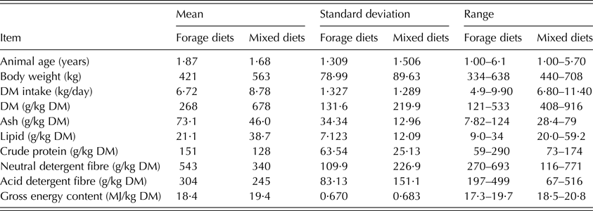
The experimental data used for evaluation is summarized in Table 1. As individual animal data were not available in all cases, treatment means were used. The model was evaluated for DMP, GEI and MY by comparing observed v. predicted values using mean square predicted error (MSPE) (Eqn (3)).
 $${\rm MSPE} = \; \mathop \sum \limits_{i = 1}^n (O_i - \; P_i)^2\; /n$$
where O i and P i are the observed and predicted values, respectively. The MSPE was then decomposed into mean bias, slope bias and random bias following Bibby & Toutenberg (Reference Bibby and Toutenberg1977). The square root of the MSPE (RMSPE) estimates the overall prediction error in the same unit as the observed values. The ratio of the RMSPE to the standard deviation of the observations (RSR) was also used to assess model predictions by taking into account the variability of observations, where values closer to zero, indicating less residual variation, are considered better than values closer to or greater than one (Moriasi et al. Reference Moriasi, Arnold, Van Liew, Bingner, Harmel and Veith2007). Weighted MSPE (MSEPw) values were calculated as described in Appuhamy et al. (Reference Appuhamy, France and Kebreab2016) (Eqn (4)), where O i and P i are the ith observed and predicted values, respectively, n is the number of observations, and SD i is the standard deviation of the ith treatment mean. This allowed for assessment of prediction error where data with more uncertainty is given less weight. Both RMSPE and RMSPEw were reported as percentages of the observed mean, to create a comparable scale that allowed for comparison of error in terms of the magnitude of the observed values.
 $${\rm MSPEw} = \; \mathop \sum \limits_{i = 1}^N (O_i - \; P_i)^2 \times \displaystyle{{(1/SDi)} \over {\left( {\sum\nolimits_{i = 1}^N {(1/SDi)}} \right)}}\; \; $$
Mean and range of observed chemical composition, intake and animal characteristics from experiments used in model evaluation, split by forage diets (n = 19) v. mixed diets (n = 16)
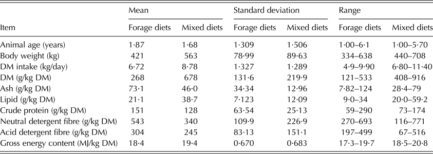
DM, dry matter.
Lin's concordance correlation coefficient (CCC) was calculated, decomposed into the Pearson correlation coefficient, r, which measures precision, and the bias correction factor, C b , which indicates accuracy in terms of deviation from the slope of unity, and used to compare models (Lin Reference Lin1989; Tedeschi Reference Tedeschi2006).
The AusBeef model was evaluated for DMP, GEI and MY and compared with the empirical predictions provided by the NASEM (2016) model, version 1.037.9, as available for download from the NASEM website, and the mechanistic L2 level of solution of the RNS model (Tedeschi & Fox Reference Tedeschi and Fox2016) version 0.5.6288.22826.
The NASEM (2016) empirical level of solution calculates CH4 production from a series of empirical equations (Mills et al. Reference Mills, Kebreab, Yates, Crompton, Cammell, Dhanoa, Agnew and France2003; IPCC Reference Eggleston, Buendia, Miwa, Ngara and Tanabe2006; Ellis et al. Reference Ellis, Kebreab, Odongo, McBride, Okine and France2007, Reference Ellis, Kebreab, Odongo, Beauchemin, McGinn, Nkrumah, Moore, Christopherson, Murdoch, McBride, Okine and France2009; Ricci et al. Reference Ricci, Rooke, Nevison and Waterhouse2013; Moraes et al. Reference Moraes, Strathe, Fadel, Casper and Kebreab2014; Escobar-Bahamondes et al. Reference Escobar-Bahamondes, Oba and Beauchemin2017). The NASEM model reports the median values for DMP and CH4 yield as part of the CH4 reports page, which was then compared with predictions from AusBeef as well as values reported in the literature. Gross energy intake is calculated internally in the model and reported on the CH4 reports page.
The RNS model is a dynamic, mechanistic model for prediction of large and small ruminant performance that derives its structure from the Cornell Net Carbohydrate and Protein System model for cattle and small ruminants (Fox et al. Reference Fox, Sniffen, O'Connor, Russell and Van Soest1992, Reference Fox, Tylutki, Van Amburgh, Chase, Pell, Overton, Tedeschi, Rasmussen and Durbal2000, Reference Fox, Tedeschi, Tylutki, Russell, Van Amburgh, Chase, Pell and Overton2004; Russell et al. Reference Russell, O'Connor, Fox, Van Soest and Sniffen1992; Sniffen et al. Reference Sniffen, O'Connor, Van Soest, Fox and Russell1992; O'Connor et al. Reference O'Connor, Sniffen, Fox and Chalupa1993; Tedeschi et al. Reference Tedeschi, Chalupa, Janczewski, Fox, Sniffen, Munson, Kononoff and Boston2008; Tylutki et al. Reference Tylutki, Fox, Durbal, Tedeschi, Russell, Van Amburgh, Overton, Chase and Pell2008). In the RNS model, DMP is calculated as a function of Prp production in the rumen using the stoichiometry of Wolin (Reference Wolin1960) and CH4 calculation logic of Pitt et al. (Reference Pitt, Van Kessel, Fox, Pell, Barry and Van Soest1996) without adjustments for rumen pH, and is reported with or without the inclusion of the impact of lactate fermentation. Methane production from VFA + lactate was used in evaluation and GEI was calculated internally and reported for each ingredient and the complete ration. Neither AusBeef nor the RNS report MY, so yield was calculated from model predictions of GEI and DMP for both models.
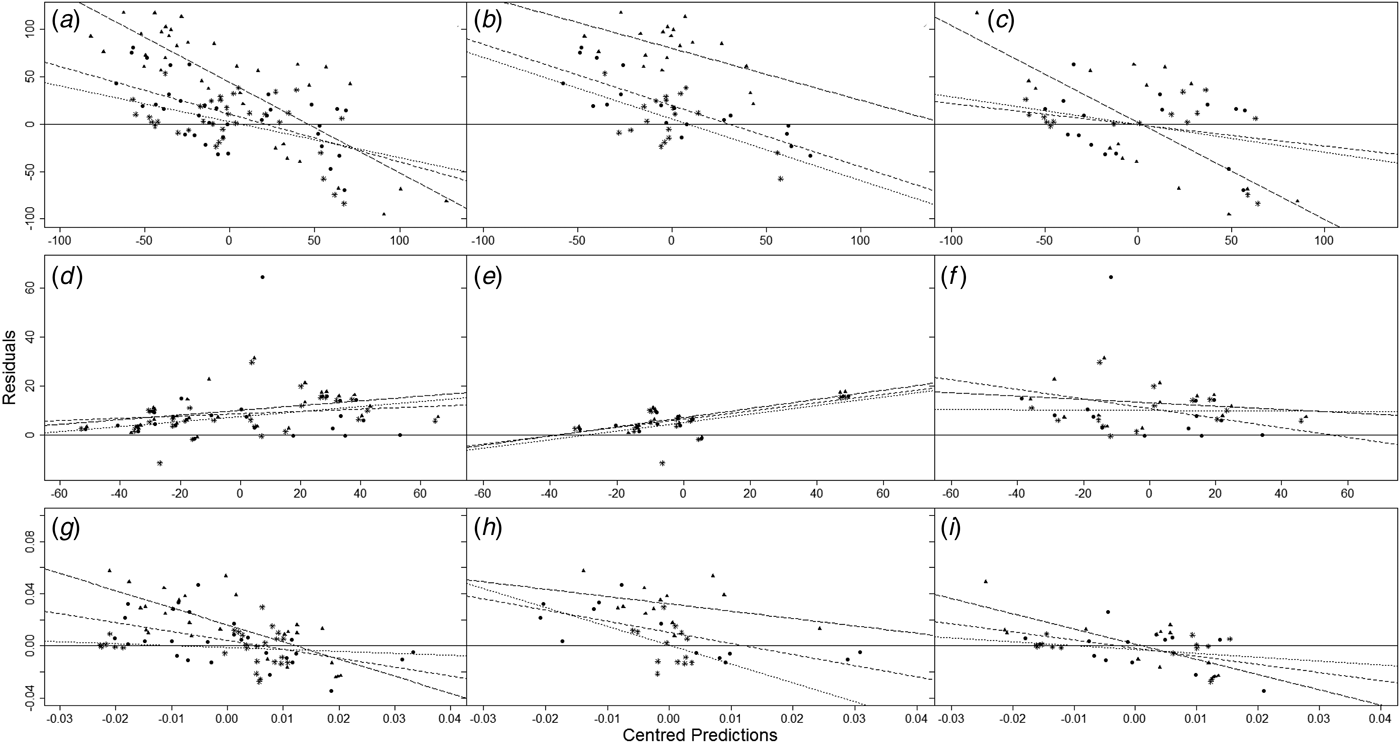
Residuals were plotted v. centred predictions for DMP, GEI and MY for the full data set and also for mixed and forage diets. Trend lines were added to show the linear regression of residuals v. centred predictions, y = ax + b, for each model. This was done to show the relationship between predicted values and residuals as well as to display diet-specific differences and help illustrate mean and slope bias.
RESULTS
AusBeef v. National Academies of Sciences, Engineering and Medicine (2016) and Ruminant Nutrition System (Tedeschi & Fox Reference Tedeschi and Fox2016) for daily methane production, gross energy intake and methane yield
Prediction of daily methane production
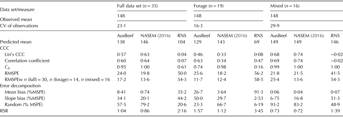
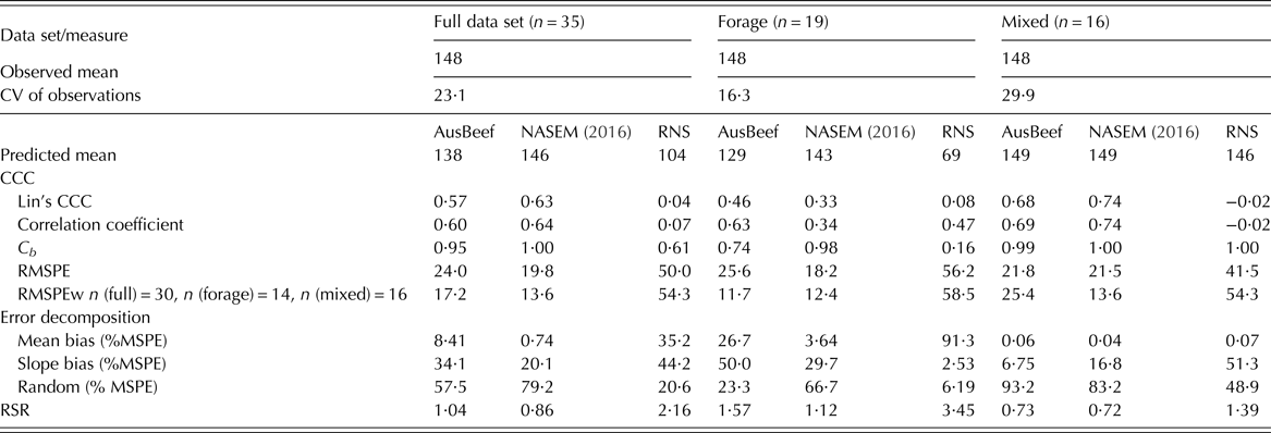
For DMP (Figs 1(a) to (c); Table 2), the observed means were similar for forage and mixed diets, although mixed diets had a higher coefficient of variation (CV) than forage diets. In general, AusBeef performed closer to NASEM than RNS. For the full data set, all models had at least 20% slope bias, though the majority of error for AusBeef and NASEM was random for the full and mixed data sets. The majority of non-random bias was primarily slope bias for all models and diets, with the exception of RNS on forage diets, where 91·3% of bias was due to mean bias. Mean bias increased on forage diets for NASEM and AusBeef as well. When expressed as a percentage of the observed mean, RMSPE and RMSPEw were similar for AusBeef and NASEM, while the RNS model had a consistently higher RMSPE, RMSPEw and RSR. The NASEM model had the smallest RSR in all cases. NASEM had the highest CCC for the full and mixed data sets, while AusBeef had the highest CCC for forage diets, though both models behaved similarly. For all models, C b was highest for mixed diets, as was the CCC for AusBeef and NASEM. AusBeef had C b ⩾ 0·74 for all data sets, and ⩾0·95 for full and mixed data sets, indicating less deviation from the slope of unity and higher accuracy of prediction.
Residuals v. centred predictions for daily methane production (g/day, top row, graphs a–c), gross energy intake (MJ/day, middle row, graphs d–f), and methane yield MJ CH4/MJ GEI, bottom row, graphs g–i). Leftmost row represents full data set, middle row represents forage diets and rightmost row represents mixed diets. ● and ----- are AusBeef, * and ····· are NASEM (2016) empirical, and ▲ and – – – – are RNS. Dashed lines represent trend line for linear regression y = ax + b for each model.

Evaluation of AusBeef, NASEM ( 2016 ) and RNS (Tedeschi & Fox Reference Tedeschi and Fox2016 ) models in their prediction of daily methane production (g/day)
RNS, Ruminant Nutrition System; CV, coefficient of variation (%); Lin's CCC and decomposition calculated as in Tedeschi (Reference Tedeschi2006); RMSPE, square root of mean square prediction error (% of observed mean); RMSPEw, square root of weighted mean square prediction error (% of observed mean); RSR, ratio of the root square mean prediction error to the standard deviation of the observations. Not all diets reported standard deviation or standard error of methane yield, therefore n is given separately for weighted RMSPE.
Slope bias ranged from 2·53 to 50·00%. The RNS model had a greater slope bias for the full and mixed data sets and a higher mean bias overall. AusBeef had greater mean bias than NASEM, but similar slope bias. All models had lower RSR and higher random error for mixed diets than for other data sets. For all models and data sets, slope bias was negative, while mean bias was >0 for the full and forage data sets, and closest to zero for the mixed data set.
In general, models underpredicted DMP for the full data set, with RNS underpredicting for the most diets and AusBeef for the least, though residuals for NASEM were clustered closer to zero than those of the other two models. AusBeef and RNS overpredicted CH4 emissions most often for mixed diets. The RNS model underpredicted DMP for all forage diets, though all models underpredicted DMP more often on forage diets than mixed, while the distance between maximum overprediction and maximum underprediction was greatest for mixed diets even though overall mean and slope bias was smallest. The NASEM model had consistently lower prediction error, and the RNS consistently higher, while AusBeef was intermediate but behaved closer to NASEM. AusBeef in general underpredicted CH4 emissions, less so on mixed diets than forage diets, and with a smaller unweighted MSPE and RSR for mixed diets, though the MSPEw was smallest on forage diets.
Prediction of gross energy intake
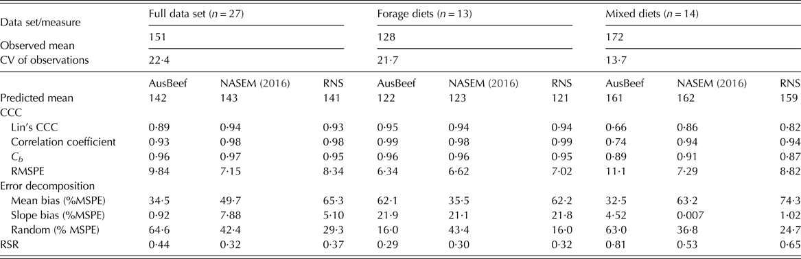
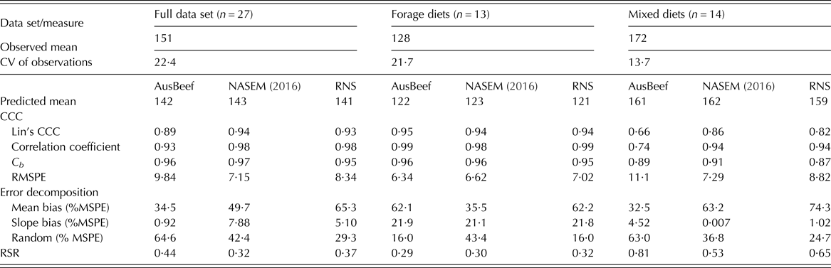
For GEI (Figs 1(d) to (f); Table 3), mixed diets had a higher observed mean but a lower CV for the observed data. All models had smaller RSR and smaller RMSPE than for either DMP or MY, but all models showed higher mean bias as a percentage of MSPE, regardless of diet. NASEM had a consistently low RSR and RMSPE for all data sets, while AusBeef had the highest RSR and RMSPE for the full and mixed data sets, and RNS model was intermediate. All models had C b ⩾ 0·87 for all models and data sets, though CCC and C b decreased for all models on the mixed data set.
Evaluation of AusBeef, NASEM ( 2016 ) and RNS (Tedeschi & Fox Reference Tedeschi and Fox2016 ) model predictions of gross energy intake (MJ/day)
RNS, Ruminant Nutrition System; CV, coefficient of variation (%); RMSPE, square root of mean square prediction error (% of observed mean); Lin's CCC and decomposition calculated as in Tedeschi (Reference Tedeschi2006); RSR, ratio of the root square mean prediction error to the standard deviation of the observations.
Slope bias was generally smaller for GEI than for DMP or MY, and all models had similar mean and slope bias for the forage data set, while AusBeef had the largest slope bias for mixed diets and the smallest slope bias for the full data set. The NASEM model had the smallest slope bias for all models and measures, −0·005 for the mixed data set of GEI. In general, all models underpredicted GEI for all data sets. AusBeef had the largest residual, due to underpredicting GEI by 30% for one diet in the mixed data set, and all models underpredicted GEI to the greatest extent on mixed diets. The majority of AusBeef's non-random error was due to mean bias, not slope bias, though this was consistent with the increased mean bias seen in other models for predictions of GEI.
Prediction of methane yield
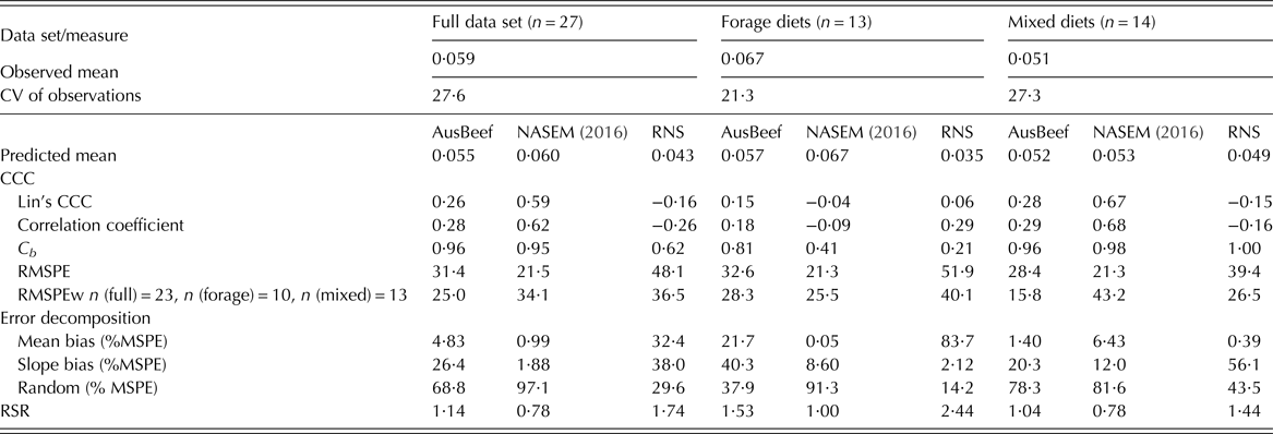
For MY (Figs 1(g) to (i); Table 4), the data displayed a higher CV than for GEI or DMP in general. Relative to DMP and GEI, AusBeef and NASEM had higher RMSPE, and AusBeef had a higher RSR for the full and mixed data sets, while the RSR for NASEM decreased for all data sets, as did the RSR for RNS for the full and forage data sets. For both AusBeef and NASEM, the majority of error was random, except for forage diets, where AusBeef had higher slope bias, which was probably related to the increases in systematic bias for forage diets seen throughout the analysis. For RNS, there was no consistent pattern to error sources, though all models showed higher mean bias for forage diets, as was also seen for GEI. Methane yield had the lowest CCC for all models and data sets, with RNS displaying a negative CCC for the full and mixed data sets due to a negative r, as did NASEM for forage diets. As seen with GEI, C b was highest for the mixed data set, and the lowest overall C b values were for MY on forage diets, as were the lowest r values, with |r| < 0·3 for all models on forage diets.
Evaluation of AusBeef, NASEM ( 2016 ) and RNS (Tedeschi & Fox Reference Tedeschi and Fox2016 ) model predictions of methane yield MJ (CH4/MJ gross energy intake)
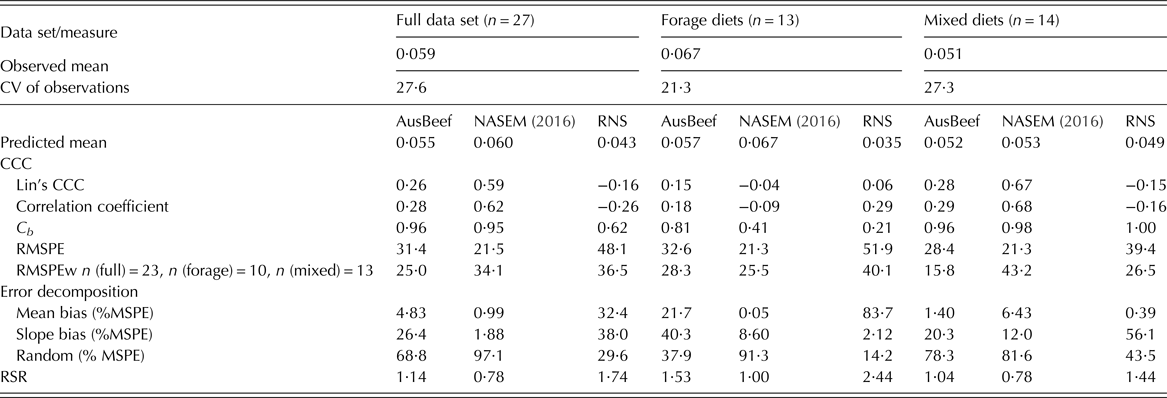
RNS, Ruminant Nutrition System; CV, coefficient of variation (%); Lin's CCC and decomposition calculated as in Tedeschi (Reference Tedeschi2006); RMSPE, square root of mean square prediction error (% of observed mean); RMSPEw, square root of weighted mean square prediction error (% of observed mean); not all diets reported standard deviation or standard error of methane yield, therefore n is given separately for weighted RMSPE.
Mean bias was smaller for MY than for DMP or GEI, and while NASEM had the smallest mean bias for the full and forage data sets and the largest slope bias for forage diets, RNS had the smallest mean bias and greatest slope bias for mixed diets. The empirical NASEM model overpredicted MY more often than RNS or AusBeef, and the proportion of diets overpredicted by NASEM was 0·52, 0·46 and 0·57 for the full, forage and mixed data sets, respectively. For forage diets, the RNS model underpredicted MY for all diets, and the proportion of diets underpredicted was 0·88 for the full data set. When average prediction error was compared, all models underpredicted MY on average for the full and forage data sets and overpredicted MY for the mixed data set. In general, AusBeef had a higher CCC and smaller RMSPE and RSR for mixed diets than for forage diets, as well as less slope and mean bias.
DISCUSSION
AusBeef is a mechanistic model that requires detailed feed information, preferably on a per ingredient basis, to parameterize diet inputs to the model. One of the major limitations of the current analysis was the scarcity of studies in the literature that had sufficient animal, diet and feed intake information for the entire CH4 measurement period. Therefore, any missing data had to be filled in from literature sources, which may vary significantly from feed type and region where the study was conducted. This contributed to model error for all three models analysed, as the RNS also relies on similar detailed feed information, as does the NASEM. Lack of such data is an issue previously identified in the literature as a major area to be targeted for improving representativeness and accuracy of biological models (McNamara et al. Reference McNamara, Hanigan and White2016). For complex, mechanistic models such as AusBeef and RNS, a simplification of feed inputs required may be warranted, but at the cost of mechanistic representation of rumen function, an issue which requires further discussion before changes are to be made.
In general, systematic bias, particularly mean bias, increased for all models on forage diets. The majority of error for the AusBeef and NASEM models was random. The RNS model had higher systematic bias, and consistently higher mean bias for prediction of GEI, while slope bias predominated for DMP and MY. Systematic bias for AusBeef was primarily due to slope bias, and due to mean bias for NASEM. AusBeef trended more closely with NASEM than with RNS in terms of error decomposition and overall magnitude of RSR and RMSPE, both weighted and unweighted. While C b for the RNS model for DMP on mixed diets was equal to 1, indicating high accuracy, r was −0·02, indicating very little linear relationship between observed and predicted values, and therefore less precision. Similar behaviour was observed for all models for MY, where |r| was <0·3 in all cases for AusBeef and RNS, and for NASEM on forage diets, indicating that precision varied more than accuracy. While reproducibility was higher for GEI than DMP or MY, particularly on forage diets, for all models, r varied more than C b , indicating that precision varied more than accuracy, leading to a greater risk of unrealistic predictions.
Of the mechanistic models evaluated, AusBeef had a consistently lower RSR and RMSPE than RNS, except for the full and mixed data sets of GEI. AusBeef also displayed higher reproducibility than RNS, as measured by CCC, except for GEI on mixed diets, though NASEM had the highest CCC values for the mixed and full data sets across all measures. For DMP and MY, RSR values for RNS were approximately twice that of AusBeef, and RMSPE and RMSPEw were higher for RNS than AusBeef, indicating that AusBeef was better able to capture the variation of the observed data in its predictions. However, both models require improvement in predicting DMP and MY, as evidenced by RSR values >1. AusBeef had greater accuracy and less prediction error on mixed diets, though AusBeef performed better for predicting GEI on forage diets than on mixed, and overall performance was most similar to that of NASEM in general.
The prediction of enteric CH4 emissions can be used to evaluate the efficacy of different management schemes in reducing enteric CH4 while maximizing animal productivity. As mechanistic modelling of CH4 production develops further, it is possible that other feed additives could be evaluated for their potential to reduce methanogenesis in the rumen and be incorporated into future mechanistic models. For example, the effects of ionophores on microbial population and VFA production patterns in the rumen could be added, or an explicit methanogen pool could be included, such as the H2–methanogen model of Wang et al. (Reference Wang, Janssen, Lynch, van Brunt and Pacheco2016). Explicit inclusion of methanogens in dynamic rumen models would then allow for modelling the effects of methanogen-targeting additives such as 3-nitrooxypropanol (Haisan et al. Reference Haisan, Sun, Guan, Beauchemin, Iwaasa, Duval, Barreda and Oba2014). These sub-models could then be incorporated into mechanistic models to bring models more in line with current beef production practices.
When evaluated using independent data and compared with the empirical NASEM and the mechanistic RNS models, AusBeef showed promise in predicting DMP, particularly for mixed diets, with low systematic error and adequate reproducibility, as well as mean and slope bias comparable to that of NASEM. AusBeef also performed well at predicting GEI and DMI, with higher reproducibility and lower RSR on forage diets than mixed diets, perhaps indicating that some re-evaluation of internal calculations of DMI and GEI prediction may be needed to further improve model predictions on mixed diets. However, because of the relatively small error in predicting DMI and GEI compared with CH4, further updates to AusBeef should be focused on CH4 calculation and H2 balance in the rumen.
As MY exhibited greater error and poorer precision than DMP or GEI, it is possible that the error in MY for all models is due to a combination of the errors of the two model outputs used to calculate the yield, which should be taken into account in future analyses of model predictions of MY. However, greater error in predicting MY as opposed to DMP has been seen in other models, such as the modified version of MOLLY used to represent enteric CH4 emissions from sheep (Vetharaniam et al. Reference Vetharaniam, Vibart, Hanigan, Janssen, Tavendale and Pacheco2015). Therefore, this may be a feature of modelling CH4 production itself that should be addressed in the future.
Among the two mechanistic models compared, AusBeef predictions fit observed data better than those of RNS, with less systematic bias and lower weighted and unweighted RMSPE. The RNS consistently underpredicted DMP and MY, particularly for forage diets, though prediction error was less for mixed diets, as was seen with AusBeef. In general, the empirical NASEM model had higher reproducibility and lower RSR and RMSPE, particularly for the full and mixed data sets, as well as less mean and slope bias, indicating better prediction fit relative to observed data, particularly for forage diets. The RSR values closer to 1 and increased systematic bias for forage diets indicate that all models may benefit from further improvement in the representation of forage diets. In many cases, for all models, r varied more than C b between data sets and measures and was smaller in magnitude. This suggests that precision varied more than accuracy, leading to a greater risk of unrealistic predictions.
CONCLUSIONS
AusBeef's optimization specifically for beef cattle on feedlot diets allows it to represent CH4 production on mixed diets with similar performance to that of the current beef NASEM model, and provides a valuable addition to the current set of mechanistic models in use by researchers and producers. Further studies are required to improve the prediction of CH4 on forage diets.
Supplementary material
The supplementary material for this article can be found at https://doi.org/10.1017/S0021859617000429.
The authors acknowledge funding from the Department of Agriculture, Fisheries and Forestry, ‘Filling the Research Gap’ round 2 and partial funding was provided by the Sesnon Endowed Chair Program at the University of California, Davis as well as the James Beard Foundation National Scholars Program. The earlier development of AusBeef for feedlots was partially funded by the Commonwealth Scientific and Industrial Research Organization and Meat and Livestock Australia and Grains Research and Development Corporation. David Pacheco was funded by the Ministry for Primary Industries, New Zealand in support of the objectives of the Global Research Alliance on Agricultural Greenhouse Gases. Research was conducted at the University of California, Davis, 1 Shields Avenue, Davis, CA 95616, USA.