1. Introduction
Classical scaling arguments such as those of Kolmogorov, Oboukhov and Corrsin, hereafter referred to collectively as KOC (Kolmogorov Reference Kolmogorov1941; Oboukhov Reference Oboukhov1941a ,Reference Oboukhov b , Reference Oboukhov1949; Corrsin Reference Corrsin1951; Kolmogorov Reference Kolmogorov1962; Oboukhov Reference Oboukhov1962), are the basis for many turbulence theories and models. It is valuable for the general understanding of turbulence to know the conditions under which the KOC hypotheses hold. Here, simulated flows are considered which are homogeneous and axisymmetric but strongly affected by a stabilising density gradient. The term ‘axisymmetric’ refers to the statistics being independent of direction on a horizontal plane rather than to a cylindrical domain.
As noted by Riley & Lindborg (Reference Riley and Lindborg2008), if the buoyancy force is important then some of the assumptions of KOC are not met. On the other hand, the
 $-5/3$
slope in the horizontal velocity spectra observed in simulations of stratified turbulence more than a decade ago (Riley & de Bruyn Kops Reference Riley and de Bruyn Kops2003) encourages the thought that KOC scaling might be relevant, an idea supported by the geophysical measurements reviewed by Riley & Lindborg (Reference Riley and Lindborg2008). Lindborg (Reference Lindborg2006) hypothesises that KOC scaling of the spectra holds with roughly the textbook values for the leading multiplicative coefficients. More recent simulations, though, indicate that, while the slope of the velocity spectrum appears to be
 $-5/3$
over some range of wavenumbers, the slope of the corresponding longitudinal structure function is
 $2/3$
over only part of the corresponding range of separation distances (Almalkie & de Bruyn Kops Reference Almalkie and de Bruyn Kops2012b
). Statistical analyses suggest that spectra may be more reliable than structure functions for estimating power laws in turbulence (Nichols-Pagel et al.
Reference Nichols-Pagel, Percival, Reinhall and Riley2008), and it is well recognised that one-dimensional spectra alias energy to larger length scales while structure functions aggregate energy below a given length scale (Townsend Reference Townsend1956; Davidson & Pearson Reference Davidson and Pearson2005). Nevertheless, it is worthwhile to consider implications of KOC scaling beyond those that apply to spectra.
The purpose of this paper is to investigate the extent to which turbulence subjected to strong stabilising stratification satisfies KOC scaling laws, and also to examine the intermittency exponent for consistency with literature values for unstratified turbulence. Before considering any of this, though, it is important to consider the question of scale separation, or what Gregg (Reference Gregg1987) refers to as the ‘bandwidth of length scales available to turbulence’. For unstratified turbulence, it has long been known that the Reynolds number has to be sufficiently high in order for simulation results and theory to compare favourably. Just how high is quantified by Yeung, Donzis & Sreenivasan (Reference Yeung, Donzis and Sreenivasan2005), who show that simulations of scalar transport in isotropic homogeneous turbulence satisfy the classical scaling laws only if the Taylor Reynolds number is greater than approximately 240.
In simulations of stratified turbulence, the challenge of providing sufficient scale separation is complicated by the introduction of the Ozmidov length scale below which three-dimensional turbulence is not expected to be strongly influenced by the buoyancy force. The ratio of the Ozmidov,
 $L_{o}$
, and Kolmogorov,
 ${\it\eta}$
, length scales is related to the buoyancy Reynolds number
 $\mathit{Re}_{b}\equiv (L_{o}/{\it\eta})^{4/3}$
. The definition of
 ${\it\eta}$
follows from Kolmogorov’s first hypothesis that the statistics of the small scales are uniquely determined by
 ${\it\nu}$
and
 $\langle {\it\epsilon}\rangle$
. The Ozmidov length scale
 $L_{o}$
can be interpreted as the length scale determined by mean turbulence kinetic energy
 $\langle {\it\epsilon}\rangle$
and the buoyancy frequency
 $H$
, but not the kinematic viscosity
 ${\it\nu}$
(Riley & Lindborg Reference Riley and Lindborg2008). This suggests that one or both definitions may not be relevant unless
 $\mathit{Re}_{b}$
is high, an observation we return to in § 7. For theoretical and computational analyses of the relationship between Reynolds numbers and the buoyancy Reynolds number in the strongly stratified regime, see Riley & de Bruyn Kops (Reference Riley and de Bruyn Kops2003) and Hebert & de Bruyn Kops (Reference Hebert and de Bruyn Kops2006a
) respectively.
For one decade of length scales to be available for turbulence to form,
 $\mathit{Re}_{b}=21.5$
(Hebert & de Bruyn Kops Reference Hebert and de Bruyn Kops2006a
). Gibson (Reference Gibson and Nihous1980), assuming isotropic turbulence and a transition to turbulence at Richardson
 $\text{number}=1/4$
, found
 $\mathit{Re}_{b}\approx 30$
for active turbulence to form. This value of
 $\mathit{Re}_{b}$
is supported experimentally by Stillinger, Helland & Atta (Reference Stillinger, Helland and Atta1983). Shih et al. (Reference Shih, Koseff, Ivey and Ferziger2005) compare several common overturning length scales with the Ellison scale for
 $0.1<\mathit{Re}_{b}<1000$
, demonstrating ranges of applicability for each length scale examined. Recently, Bartello & Tobias (Reference Bartello and Tobias2013) concluded that care must be taken when drawing conclusions from stratified flow spectra unless
 $\mathit{Re}_{b}>O(10)$
.
One reason for emphasising scale separation is that for this study the large scales are synthetically introduced into the simulations to produce simple flows, as explained in § 2. This practice is fairly common in the study of stratified turbulence with forced simulations (Lindborg Reference Lindborg2006; Brethouwer et al. Reference Brethouwer, Billant, Lindborg and Chomaz2007; Waite Reference Waite2011; Kimura & Herring Reference Kimura and Herring2012) or decaying simulations (Godeferd & Staquet Reference Godeferd and Staquet2003; Riley & de Bruyn Kops Reference Riley and de Bruyn Kops2003; Bartello & Tobias Reference Bartello and Tobias2013). In order to infer the dynamics of a physical flow from the simulations, one has to assume that the dynamics of interest are not determined by the details of the large scales. Exactly this assumption is made in each of the KOC scaling hypotheses, and the basis for it is large-scale separation.
In fact, scale separation is one of two principal assumptions common to all of the KOC scaling hypotheses. Sometimes one sees reference to the concept of a ‘Kolmogorov cascade’, which would raise theoretical questions if applied to a stratified flow in which there are interactions between kinetic and potential energy at various length scales that are more nuanced than a simple downscale cascade. This does not matter for the present analysis because, as noted by Kholmyansky & Tsinober (Reference Kholmyansky and Tsinober2008), ‘neither the original nor all the subsequent derivations of
 $4/5$
law use the assumption on locality of interactions and the existence of cascade’. We add to this that assumptions about how energy transfers between scales is not part of the refined scaling hypotheses (Kolmogorov Reference Kolmogorov1962; Oboukhov Reference Oboukhov1962) either.
The other principal assumption in all of the KOC scaling hypotheses is local isotropy. For stratified flows at low Reynolds number, Godeferd & Staquet (Reference Godeferd and Staquet2003) show that the velocity derivatives are not isotropic. Hebert & de Bruyn Kops (Reference Hebert and de Bruyn Kops2006b
) report that the local strain rates quickly approach the isotropic limit as
 $\mathit{Re}_{b}$
increases above
 $O(1)$
in stratified turbulence with no imposed mean shear, but even with
 $\mathit{Re}_{b}\approx 15$
the flows are measurably anisotropic at the small scales. When there is mean shear, Smyth & Moum (Reference Smyth and Moum2000) also observe the small scales approaching isotropy, but at a much higher buoyancy Reynolds number. Given sufficient scale separation, it can be expected that isotropy will improve as the length scale of interest decreases, but several factors complicate consideration of isotropy relative to KOC scaling. One is that any finite sample of a flow will exhibit some anisotropy. A second complication is that some flows may be consistent with KOC scaling even if they cannot be locally isotropic due to, say, a mean gradient of velocity or scalar (Warhaft Reference Warhaft2000; Durbin & Pettersson Reif Reference Durbin and Pettersson Reif2010). This is particularly relevant to stratified flows in which there is a mean scalar gradient by definition. Yet isotropic homogeneous turbulence with a mean gradient in a passive scalar exhibits KOC scaling in that scalar (Yeung, Xu & Sreenivasan Reference Yeung, Xu and Sreenivasan2002) despite the local scalar derivatives being markedly anisotropic. Indeed, Augier, Sébastien & Billant (Reference Augier, Sébastien and Billant2012) derive the Kolmogorov relations for stratified turbulence without assuming local isotropy.
Based on the foregoing, it is postulated that the simulations of Almalkie & de Bruyn Kops (Reference Almalkie and de Bruyn Kops2012b
) may have sufficient scale separation for studying classical turbulence scaling. For this paper, the resolution of those simulations has been increased to as high as
 $8192\times 8192\times 4096$
to ensure the fidelity of higher-order statistics. Nevertheless, the dynamic range enables only a limited Reynolds number, and the velocity fields in these simulations cannot be perfectly locally isotropic due to finite sample size, and the scalar fields cannot be perfectly isotropic for this reason and because of the mean stratification (Warhaft Reference Warhaft2000). Therefore, an unstratified benchmark simulation is used which has the same dynamic range as the stratified case and which approaches local isotropy and KOC scaling about as well as any simulations reported in the literature do. This simulation is of nominally isotropic homogeneous turbulence, with a mean scalar gradient, at a Taylor Reynolds number of 400 resolved on
 $8192\times 8192\times 8192$
grid points.
An overview of the simulations is presented in the next section, with local isotropy evaluated in § 3 as a prelude to investigating the classical scaling hypotheses. Then, in § 4, the spectra and second- and third-order structure functions of the velocity and scalar fields are examined to evaluate consistency with KOC scaling. The local kinetic and scalar energy dissipation rates are examined in § 5 and then the locally averaged dissipation rates are considered in the context of Kolmogorov’s refined similarity hypotheses in § 6. Finally, conclusions are summarised in § 7.
2. Numerical simulations
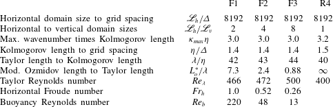
Four direct numerical simulations are analysed for this research. Three are of axisymmetric homogeneous stratified turbulence configured the same as those reported by Almalkie & de Bruyn Kops (Reference Almalkie and de Bruyn Kops2012b ) but are different realisations with finer spatial resolution. The fourth is an unstratified isotropic homogeneous case with a uniform mean scalar gradient. The velocity fields are in the same series as those reported by Almalkie & de Bruyn Kops (Reference Almalkie and de Bruyn Kops2012a ) but at higher Reynolds number. The parameters for all the simulations are given in table 1.
Simulation parameters.

The stratified data are solutions to the three-dimensional Navier–Stokes equations and thermal energy equation with the non-hydrostatic Boussinesq approximation. The mean velocities and the mean density gradient are constant, which allows the fluctuating quantities to be computed in a triply periodic cuboid domain using a pseudo-spectral method with fractional time stepping. The grid spacing is the same in each direction, as are the outer dimensions in the two horizontal directions. The outer dimension in the vertical varies with the Froude number simulated.
The stratified fields are initially quiescent and then numerical forcing is applied until statistically stationary axisymmetric homogeneous stratified turbulence is observed. The forcing energy is applied using the deterministic schema denoted ‘Rf’ by Rao & de Bruyn Kops (Reference Rao and de Bruyn Kops2011). Briefly, energy is added to the horizontal velocity components at the smallest horizontal wavenumbers to maintain a prescribed spectrum for the horizontal kinetic energy. The target spectrum was determined by using a stochastic forcing technique similar to that of Lindborg (Reference Lindborg2006). A very small amount of energy is also added randomly to the horizontal components of velocity at small vertical wavenumbers to induce shear instabilities. The forcing is applied until statistical stationarity is observed and then maintained for approximately one large-eddy turnover time to assure convergence, as discussed by Almalkie & de Bruyn Kops (Reference Almalkie and de Bruyn Kops2012b ).
The three stratified cases are denoted F1, F2 and F3 and can be characterised as strongly, more strongly and very strongly stratified. A Froude number
 $\mathit{Fr}_{h}$
based on the horizontal correlation length scale and the root-mean-square (r.m.s.) of the horizontal velocity is included here in table 1, but an array of metrics regarding the strength of the stratification is tabulated in Almalkie & de Bruyn Kops (Reference Almalkie and de Bruyn Kops2012b
). Importantly, the buoyancy Reynolds numbers
 $\mathit{Re}_{b}$
span a value of approximately 30, the possible relevance of which is discussed in § 1. The length scale
 $L_{o}^{\ast }\equiv (\langle {\it\epsilon}\rangle /(N/2{\rm\pi})^{3})^{1/2}$
is the Ozmidov length scale with the factor of
 $2{\rm\pi}$
retained in the conversion between frequency and period. The utility of this length scale for flows with limited dynamic range is discussed in Almalkie & de Bruyn Kops (Reference Almalkie and de Bruyn Kops2012b
).
The isotropic homogeneous simulation is denoted R4 and is the next higher in Reynolds number in the series of simulations R1, R2 and R3 in Almalkie & de Bruyn Kops (Reference Almalkie and de Bruyn Kops2012a
). The velocity field is forced isotropically so that the three-dimensional kinetic energy spectrum at length scales larger than the integral length scale matches Pope’s model spectrum with his
 $p_{0}=2$
and his
 $c_{L}=6.78$
(Pope Reference Pope2000, (equation (6.247))). The passive scalar field is forced simply by including a term in the scalar transport equation that represents a mean gradient. Features of this simulation relevant to the current study are that the Taylor Reynolds number is well above the value often cited as the threshold for studying turbulence at high Reynolds number (Yeung et al.
Reference Yeung, Donzis and Sreenivasan2005), the small-scale resolution relative to the Kolmogorov length scale is comparable to that in the stratified cases, and the dynamic range is comparable to that in the stratified cases. In short, in all four simulations there are approximately three decades of scale separation between the largest and smallest length scales of turbulence, and the grid resolution is finer than the Kolmogorov length scale.
Throughout this paper, the domain-averaged dissipation rate of turbulence kinetic energy,
 $\langle {\it\epsilon}\rangle$
, and the corresponding rate of diffusive destruction of scalar variance,
 $\langle {\it\chi}\rangle$
, are used in the descriptions of the flows, beginning with the definitions of the Taylor microscale and Kolmogorov length scale implicit in table 1. Since
 $\langle {\it\epsilon}\rangle$
and
 $\langle {\it\chi}\rangle$
are important quantities in classical turbulence theory, they are obvious starting points in the analysis of stratified turbulence without implying that, e.g., the KOC hypotheses hold.
3. Local isotropy
Local isotropy implies specific relationships among the velocity derivatives and among the scalar derivatives that can be quantified in terms of invariants that do not change with the rotation of coordinates (Siggia Reference Siggia1981; Hierro & Dopazo Reference Hierro and Dopazo2003). These invariants provide a precise way to evaluate, for instance, how closely a nominally isotropic flow approaches isotropic perfection. For our current purposes, we simply want to know how reasonable it is to apply the assumption of local isotropy to stratified turbulence, which is strongly anisotropic at large scales. The approach is to compare measures of the probability distributions of the derivatives with their isotropic limits and with the benchmark case R4.
3.1. Velocity derivatives
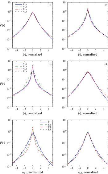
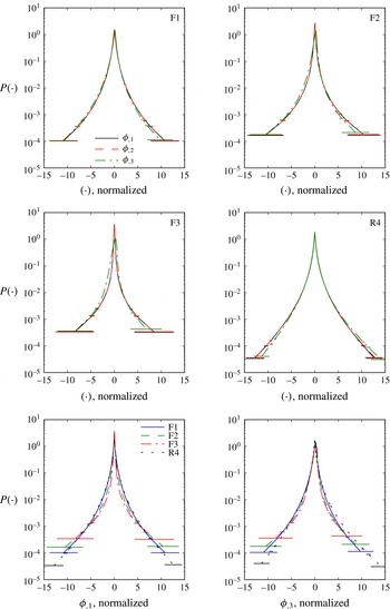
In axisymmetric homogeneous stratified turbulence there are five statistically independent local velocity derivatives. The probability density functions (p.d.f.s) of four are plotted in the first two rows of figure 1, with the notation
 $u_{i,j}$
meaning that
 $i$
is the velocity component and
 $j$
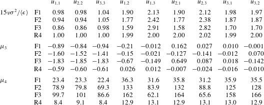
is the derivative direction, with index 3 denoting the direction parallel to gravitational acceleration. Each point represents the mean value for a bin with 16 777 216 samples. The r.m.s. of the fluctuations of the values in each bin about the bin mean provides an estimate of the statistical uncertainty that can be plotted as a horizontal error bar. In figure 1, the error bars are comparable to the linewidth and are not visible (cf. figure 3). The moments of the velocity derivatives are given in table 2.
The p.d.f.s of the velocity derivatives, each normalised by its own mean and standard deviation.

The variance
 ${\it\sigma}^{2}$
, skewness
 ${\it\mu}_{3}$
and kurtosis
 ${\it\mu}_{4}$
of the velocity derivatives.

Considering first the reference case R4, the longitudinal and transverse velocity derivatives are visibly different in figure 1, as expected. The variances are almost exactly isotropic, the skewness of the longitudinal derivatives is approximately −0.6, and the kurtoses indicate tails of the p.d.f.s heavier than Gaussian, all in agreement with Ishihara et al. (Reference Ishihara, Kaneda, Yokokawa, Itakura and Uno2007) and the references therein.
Using case R4 as a reference, we now consider the stratified cases, starting with F1, which has the highest buoyancy Reynolds number. As with R4, the behaviours of the longitudinal and transverse derivatives differ but there is little difference between the two longitudinal or the two transverse quantities. When
 $\mathit{Re}_{b}$
is reduced to 48 in case F2, several changes in the distributions become apparent. First, for all but
 $u_{1,3}$
the probability of values near zero increases so that the distributions, particularly
 $u_{3,1}$
, have sharp peaks. Second, the two longitudinal distributions become markedly different. This is even more obvious in case F3, for which the distribution of
 $u_{1,3}$
is similar to that in the isotropic case, whereas
 $u_{3,1}$
exhibits a sharp peak near zero. The probability of very-small-magnitude transverse derivatives of
 $u_{3}$
is almost an order of magnitude greater than that for
 $u_{1}$
. These characteristics of the p.d.f.s are due to stratified flows forming quasi-horizontal vortices, sometimes referred to as ‘pancake eddies’ (e.g. Lin & Pao Reference Lin and Pao1979), in which
 $u_{1,3}$
is dominated by shearing between these eddies. As the stratification increases, the pancakes get thinner (Billant & Chomaz Reference Billant and Chomaz2001) and the magnitudes of
 $u_{1,3}$
increase (see table 2 and Hebert & de Bruyn Kops Reference Hebert and de Bruyn Kops2006b
, figure 5), but the shape of
 $P(u_{1,3})$
does not change very much. On the other hand, the shape of
 $P(u_{3,1})$
is affected by the strength of the stratification because stratified turbulence tends to form in patches, which can be seen for a lower-resolution realisation of F3 in Almalkie & de Bruyn Kops (Reference Almalkie and de Bruyn Kops2012b
, figure 1). The regions of relative quiescence contribute to the peak of
 $P(u_{3,1})$
while the regions of more intense turbulence contribute to the tails, and this effect is more pronounced for stronger stratification.
Further analyses are made using the data in table 2. It is observed that the moments of the velocity derivatives depend on
 $\mathit{Re}_{b}$
and approach their isotropic values as
 $\mathit{Re}_{b}$
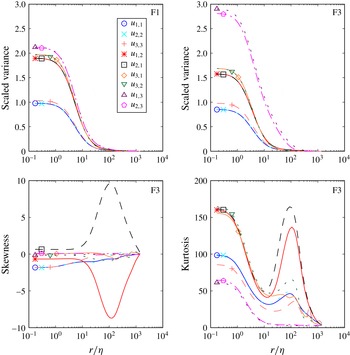
increases. The importance of the departure from isotropy is subjective, but we can make some general observations to put it into perspective. To aid in doing so, some of the moments of the derivatives averaged over spherical volumes of radius
 $r$
are shown in figure 2. These locally filtered quantities are computed in terms of Fourier series according to the unpublished derivation of Sykora, which is reproduced in the appendix of Almalkie & de Bruyn Kops (Reference Almalkie and de Bruyn Kops2012a
). Because the velocity fields in our simulations are computed in terms of finite Fourier series, the filtered quantities are exact for any averaging dimension
 $r$
up to one-half of the size of the domain.
Moments of locally averaged velocity derivatives for selected cases scaled by
 $15{\it\nu}/\langle {\it\epsilon}\rangle$
. To aid in curve identification, the symbols on the variance plots go from top to bottom in the legend in the same order as they go from top to bottom in the plot. In the online version of the paper, the symbol and line colours are the same and are unique for each derivative.

From the tabulated and graphical data for the variances, it is apparent that at low
 $\mathit{Re}_{b}$
there are three distinct groups of derivatives, whereas at higher
 $\mathit{Re}_{b}$
the data suggest two groups as in the isotropic case. The skewnesses of the longitudinal velocity derivatives are negative because the flows are statistically stationary: viscous effects continually destroy vorticity, and so there must be generation by vortex stretching, which implies negative skewness of the longitudinal derivatives (Taylor Reference Taylor1938). The skewnesses of
 $u_{1,2}$
and
 $u_{2,1}$
averaged over large
 $r$
are far from zero because of how the large scales of the flow are forced. Even as
 $r\rightarrow 0$
, though, these skewnesses include contributions from the large scales, which is consistent with them apparently asymptoting to non-zero values.
3.2. Scalar derivatives
The scalar field
 ${\it\phi}$
is the temperature in the stratified simulations and a passive scalar in simulation R4. The three spatial derivatives are
 ${\it\phi}_{,1}$
,
 ${\it\phi}_{,2}$
and
 ${\it\phi}_{,3}$
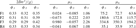
, where the first two are in the horizontal directions and statistically interchangeable. The p.d.f.s of each derivative are plotted as figure 3, and their moments are given in table 3.
The p.d.f.s of the scalar derivatives, each normalised by its own mean and standard deviation. The error bars are defined in § 3.1.

The variance
 ${\it\sigma}^{2}$
, skewness
 ${\it\mu}_{3}$
and kurtosis
 ${\it\mu}_{4}$
of the scalar derivatives;
 $D$
is the molecular diffusivity.

First, let us check the reference case R4 against the data of Yeung et al. (Reference Yeung, Xu and Sreenivasan2002) and Donzis & Yeung (Reference Donzis and Yeung2010) for unity Schmidt number and various Reynolds numbers, and more generally against the data referenced in Warhaft (Reference Warhaft2000). From the cited data, we expect the variance of
 ${\it\phi}_{,3}$
to be slightly higher than that in the directions perpendicular to the mean scalar gradient, the skewness
 ${\it\phi}_{,3}$
to be positive whereas the other skewnesses are nearly zero, and the kurtoses to indicate tails heavier than Gaussian and not strongly dependent on the direction of the derivative. It is concluded that case R4 is behaving as expected and so is a useful reference case against which to compare the stratified cases.
Next, we consider case F1. We recall that this case has Froude number of order unity and is highly non-isotropic at large scales. Nevertheless, the moments of the p.d.f.s of the local velocity derivatives are only slightly affected by buoyancy. As the buoyancy Reynolds number is reduced (cases F2 and F3), the main effect of stratification is to increase the kurtoses of all of the scalar derivatives. The same is observed for the velocity derivatives and will be considered further in the context of the local dissipation rates in § 5. Another effect of low buoyancy Reynolds number is that the vertical derivatives of the scalar are larger than the horizontal derivatives. This is expected since, in the conceptual configuration of horizontal pancake-like structures shearing against each other, the vertical derivatives will be dominant.
The bottom rows of figures 1 and 3 show how the p.d.f.s of the velocity and scalar respectively change with buoyancy Reynolds number. In each pair of plots, the horizontal derivatives are on the left and the vertical derivatives on the right. For velocity, changing
 $\mathit{Re}_{b}$
has a dramatic effect on the shape of the p.d.f. of the horizontal derivative and a minor effect on that of the vertical derivative, as discussed in § 3.1. For the scalar, the effect is minor for all derivatives. Our use of the term ‘minor’ presumes a focus on the portion of the p.d.f.s where the probability density is high, and it is noted that the logarithmic vertical axis emphasises the tails of the p.d.f.s, which are important in some applications (Sreenivasan & Antonia Reference Sreenivasan and Antonia1997). It is also noted that the horizontal axes for the scalar derivatives extend to 15 standard deviations from the mean, again because the tails are of interest to some readers. Therefore we conclude that, even with unity Prandtl number, stratification has a stronger effect on the derivatives of velocity than on those of the scalar.
The non-zero skewness of the scalar derivative parallel to the mean gradient, first observed more than 40 years ago (Gibson, Stegen & McConnell Reference Gibson, Stegen and McConnell1970), indicates that the scalar is not isotropic at small scales. In his review article, Warhaft explains the mechanism that causes the non-zero skewness and concludes that the isotropy assumption underlying KOC scaling cannot be satisfied for a scalar having a mean gradient (Warhaft Reference Warhaft2000). Nevertheless, consistency with KOC scaling for flows with a passive scalar and a mean gradient has proven useful (Yeung et al. Reference Yeung, Donzis and Sreenivasan2005). We conclude that, despite evidence of anisotropy in the data, it is worthwhile to examine KOC scaling for the stratified cases, which we do in the next section.
4. Kolmogorov–Oboukhov–Corrsin scaling
4.1. Behaviour of the velocity fields
The most commonly known classical scaling hypotheses are those presented in Kolmogorov (Reference Kolmogorov1941) and Oboukhov (Reference Oboukhov1941a
,Reference Oboukhov
b
). With the assumption that
 $\langle {\it\epsilon}\rangle$
and the kinematic viscosity
 ${\it\nu}$
determine the form of the velocity statistics in the equilibrium range, and the assumption of local isotropy, the longitudinal and transverse velocity spectra in the inertial range take the forms
 $$\begin{eqnarray}E_{11}({\it\kappa}_{1})=C_{1}\langle {\it\epsilon}\rangle ^{2/3}{\it\kappa}_{1}^{-5/3}\end{eqnarray}$$
and
 $$\begin{eqnarray}E_{22}({\it\kappa}_{1})=C_{1}^{\prime }\langle {\it\epsilon}\rangle ^{2/3}{\it\kappa}_{1}^{-5/3},\end{eqnarray}$$
and the second-order longitudinal velocity structure function takes the form
 $$\begin{eqnarray}\langle ({\it\Delta}_{r}u)^{2}\rangle =C_{2}(\langle {\it\epsilon}\rangle r)^{2/3}.\end{eqnarray}$$
The textbook values for the constants are (Pope Reference Pope2000)
 $$\begin{eqnarray}C_{1}\approx 0.49,\quad C_{1}^{\prime }\approx 0.65,\quad C_{2}\approx 2.0.\end{eqnarray}$$
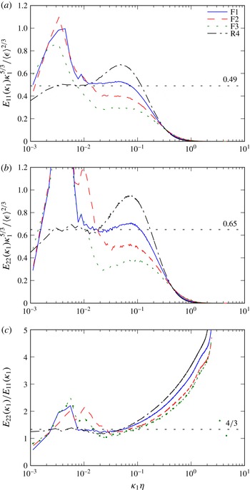
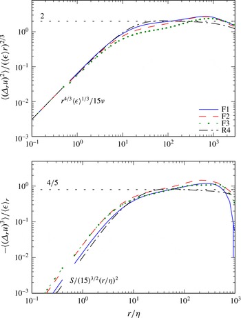
The spectra and structure function are plotted in figures 4 and 5. Full advantage of homogeneity and the statistical interchangeability of the two horizontal directions was taken in computing these quantities. Considering first the longitudinal spectra, KOC scaling collapses all the cases to a single curve in the far dissipation range. This is not obvious with the linear scaling of the ordinate in the plot of the spectra, but is evident if logarithmic scaling is used, and it is clear from the plot of the second-order structure functions. Furthermore, the third-order structure functions collapse to the relation
 $S/(15)^{3/2}(r/{\it\eta})^{2}$
for small
 $r/{\it\eta}$
, where
 $S$
is the velocity derivative skewness. The behaviours of the spectra and structure functions in the dissipation range suggest that
 ${\it\eta}$
is the appropriate length scale for studying KOC scaling rather than, say, a length scale based on the sum of
 $\langle {\it\epsilon}\rangle$
and
 $\langle {\it\chi}\rangle$
. We consider mean dissipation rates further in § 4.4.
Longitudinal and transverse velocity spectra and their ratios.

Second- and third-order longitudinal velocity structure functions. The line segments for
 $r{\it\eta}<0.6$
are not data but rather the theoretical relationships annotated on the plots.

Next, we consider the longitudinal spectra at wavenumbers smaller than the dissipation range. All the cases have a region with a plateau, so one might conclude that the scaling holds but with
 $C_{1}$
and
 $C_{1}^{\prime }$
dependent on the buoyancy Reynolds number. This is consistent with conclusions that might be drawn from figure 9 in Lindborg (Reference Lindborg2006). A closer look, though, reveals that the plateaus do not occur in the same ranges of
 ${\it\kappa}_{1}{\it\eta}$
for all cases. In cases F1 and R4, the plateau is in the vicinity of
 ${\it\kappa}_{1}{\it\eta}\approx 0.01$
, which is consistent with the laboratory data, simulations and models for unstratified turbulence (Saddoughi & Veeravalli Reference Saddoughi and Veeravalli1994; Gotoh, Fukayama & Nakano Reference Gotoh, Fukayama and Nakano2002; Meyers & Meneveau Reference Meyers and Meneveau2008). In cases F2 and F3, the plateaus occur at higher values of
 ${\it\kappa}_{1}{\it\eta}$
. The transverse spectra lead us to the same conclusions for cases F1 and R4, but for this quantity plateaus are not evident for cases F2 and F3.
To investigate further, let us consider the bottleneck effect, which appears as a bump in the near dissipation range of compensated spectra. In case R4, the bump is clearly visible at
 ${\it\kappa}_{1}{\it\eta}\approx 0.1$
, as expected (Yeung & Zhou Reference Yeung and Zhou1997; Meyers & Meneveau Reference Meyers and Meneveau2008; Donzis & Sreenivasan Reference Donzis and Sreenivasan2010). Using the same data sets as in this paper (but at lower resolution), Almalkie & de Bruyn Kops (Reference Almalkie and de Bruyn Kops2012b
) conclude that stratification impedes downscale transfer of kinetic energy, which is consistent with the smaller bump for case F1 relative to case R4. In cases F2 and F3, the bottleneck effect is not apparent in the longitudinal spectra, but is visible in the transverse spectra. The plateau regions in the longitudinal spectra for cases F2 and F3, to the extent that they might exist, are in the range of
 ${\it\kappa}_{1}{\it\eta}$
where the bottleneck effect is expected.
A consequence of Kolmogorov’s hypotheses is
 $E_{22}/E_{11}=4/3$
in the power-law range. This ratio is plotted in figure 4(c). The ratio equality is satisfied for cases R4 and F1 in the same range of wavenumbers for which plateaus appear in the spectra. For case F3, the ratio equality is not satisfied over any range of wavenumbers. For case F2, the results are not definitive; the ratio might suggest a short scaling range in the vicinity of
 ${\it\kappa}_{1}{\it\eta}\approx 0.04$
.
Putting together observations about the plateaus, the bottleneck effect and the ratio of the spectra, we arrive at the same conclusion as Bartello & Tobias (Reference Bartello and Tobias2013), namely that KOC scaling of spectra, if it occurs, does so only if there is sufficient scale separation between the Ozmidov and Kolmogorov length scales, i.e. if the buoyancy Reynolds number is high enough. Whereas it is concluded in Bartello & Tobias (Reference Bartello and Tobias2013) that
 $\mathit{Re}_{b}>O(10)$
is required for KOC scaling, the current data show that with
 $\mathit{Re}_{b}=48$
the scaling region is obscured by the bottleneck effect. Cases F2 and F3 suggest that when
 $\mathit{Re}_{b}$
is not high, a region with
 ${\it\kappa}_{1}^{-5/3}$
scaling may appear in the near dissipation range due to the competing effects of the bottleneck tending to cause a positive slope and dissipation effects tending to cause a steeply negative slope.
Lastly in our discussion of velocity spectra, we examine the numerical values of
 $C_{1}$
and
 $C_{1}^{\prime }$
. Since case F1 is close to locally isotropic and exhibits plateaus in
 $E_{11}$
and
 $E_{22}$
in the range of
 ${\it\kappa}{\it\eta}$
typical for flows that are consistent KOC scaling, we might expect it to exhibit the universal values for
 $C_{1}$
and
 $C_{1}^{\prime }$
. Indeed, the textbook constants of 0.49 and 0.65 fit the data extremely well.
Turning now to velocity structure functions, let us consider figure 5. Consistency with KOC scaling will be exhibited by a plateau in the second-order structure function at 2 and in the third-order structure function at
 $4/5$
. The isotropic case satisfies both relations almost exactly. This is an important criterion because it indicates whether a simulation has sufficient dynamic range to not just show
 ${\it\kappa}_{1}^{-5/3}$
scaling in the spectra but also to satisfy other relationships that follow from that scaling, which simulations with lower dynamic range do not do (Yeung et al.
Reference Yeung, Donzis and Sreenivasan2005). We recall that these simulations are forced and note that Antonia & Burattini (Reference Antonia and Burattini2006) show that the
 $4/5$
law is exhibited at lower dynamic range in forced than in decaying turbulence. The two most strongly stratified cases do not appear to satisfy either of the scaling relationships for structure functions. For the second-order structure function, case F1 almost plateaus at 2.0, but it appears that slightly more scale separation is needed for the plateau to be clear. The third-order structure functions, though, for the stratified cases have pronounced positive slopes in the range of
 $r/{\it\eta}$
where case R4 shows KOC scaling.
4.2. Behaviour of the scalar fields
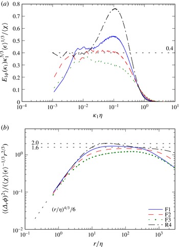
The one-dimensional horizontal scalar spectra and corresponding structure functions are shown in figure 6. The horizontal reference lines at 0.4 and 1.6 on the spectra and structure function plots respectively are based on experimental data (Sreenivasan & Kailasnath Reference Sreenivasan and Kailasnath1996). The horizontal reference line at 2.0 on the structure functions marks the plateau in simulation data of Yeung et al. (Reference Yeung, Xu and Sreenivasan2002) for comparable Reynolds and Schmidt numbers. Also shown is the asymptotic behaviour at small
 $r/{\it\eta}$
(Yeung et al.
Reference Yeung, Xu and Sreenivasan2002),
 $$\begin{eqnarray}\frac{\langle ({\it\Delta}_{r}{\it\phi})^{2}\rangle }{\langle {\it\chi}\rangle \,\langle {\it\epsilon}\rangle ^{-1/3}r^{2/3}}=\frac{1}{6}\left(\frac{r}{{\it\eta}}\right)^{4/3}.\end{eqnarray}$$
One-dimensional scalar spectra (a) and the second-order scalar structure functions (b).

The scalar spectra and structure functions confirm the conclusions drawn from the velocity data. For the unstratified case, there is a plateau in the spectrum around
 ${\it\kappa}{\it\eta}\approx 0.01$
at the ordinate value reported in the literature, and the bottleneck effect is pronounced. The data for case F1 are broadly consistent with the unstratified case, although the bottleneck effect is weaker. For cases F2 and F3 there is no bottleneck effect; there is a plateau in case F2 where the bottleneck effect is expected, and no plateau in case F3. In the plot of the structure functions, the theoretical asymptotic behaviour at low
 $r/{\it\eta}$
is evident for the cases R4 and F1; for case F3, the curve does not quite reach the asymptotic slope. This behaviour is consistent with lack of scale separation, that is, low buoyancy Reynolds number. It is also consistent with insufficient small-scale resolution to reveal the asymptotic behaviour, but this explanation is discounted since the values of
 $r/{\it\eta}$
shown on the plot are in the far dissipation range and the expected asymptotic behaviours are observed for the second- and third-order velocity structure functions. It is concluded, therefore, that effects of low buoyancy Reynolds number are observed far into the dissipation range of the scalar when
 $\mathit{Re}_{b}=13$
and not when
 $\mathit{Re}_{b}=220$
.
4.3. Yaglom relationship
Yeung et al. (Reference Yeung, Donzis and Sreenivasan2005) comment that the most important relationship in physical space that pertains to KOC scaling is that derived by Yaglom (Reference Yaglom1949) for the mixed velocity–scalar structure function:
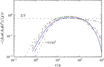
 $$\begin{eqnarray}-\frac{\langle {\it\Delta}_{r}u({\it\Delta}_{r}{\it\phi})^{2}\rangle }{\langle {\it\chi}\rangle r}=\frac{2}{3}.\end{eqnarray}$$
The appropriately scaled structure function is plotted as figure 7. As with the scalar structure functions, the expected asymptotic behaviour at low
 $r/{\it\eta}$
is observed for the unstratified case and at high
 $\mathit{Re}_{b}$
. For case F3, effects of stratification are evident in this statistic even at length scales in the far dissipation range. For all of the cases the mixed structure function peaks at approximately
 $2/3$
, although even case R4 does not show a distinct plateau; figure 3 in Yeung et al. (Reference Yeung, Donzis and Sreenivasan2005) indicates that an even higher Reynolds number is required for a clear plateau to be apparent.
The velocity–scalar structure function. Line types are the same as in figure 6.

4.4. Scaled dissipation rates
A common premise about turbulence is that
 $\langle {\it\epsilon}\rangle$
is dependent only on the size and energy of the large-scale motions in a flow (Tennekes & Lumley Reference Tennekes and Lumley1972; Sreenivasan Reference Sreenivasan1984). This is not part of the KOC hypotheses, but it is in the same vein, and so we perform the analysis on our four data sets. As noted in § 4.1, stronger stratification somewhat reduces the absolute dissipation rate of kinetic energy in simulations when the large horizontal length scales of the horizontal velocities are forced to be the same. Now let us consider the scaled dissipation rate
 $$\begin{eqnarray}\mathscr{D}=\langle {\it\epsilon}\rangle L/u_{rms}^{3}.\end{eqnarray}$$
Here,
 $L$
is an outer scale, evaluated as the average of the longitudinal integral scales of the two horizontal velocities, and
 $u_{rms}$
is the r.m.s. velocity.
For a variety of flow configurations, Sreenivasan (Reference Sreenivasan1998) report
 $\mathscr{D}$
in the range of approximately 0.5–1.0 at sufficiently high Reynolds number, but the definitions of
 $L$
and
 $u_{rms}$
vary in the literature when the flow is not isotropic. Nevertheless, it is useful to consider the values of
 $\mathscr{D}$
for the current simulations, as shown in table 4. The table also lists the values of
 $$\begin{eqnarray}\mathscr{D}_{tot}=\langle {\it\epsilon}+{\it\epsilon}_{p}\rangle L/u_{rms}^{3},\end{eqnarray}$$
where
 ${\it\epsilon}_{p}$
is the rate at which available potential energy is converted to background potential energy by molecular diffusion. The value of
 $\mathscr{D}$
for R4 is very close to the theoretical estimate of Rotta (Reference Rotta1972), but is higher than reported for a number of isotropic homogeneous simulations (Kaneda et al.
Reference Kaneda, Ishihara, Yokokawa, Itakura and Uno2003). The value for forced simulations, though, tends to be higher than that for decaying simulations (Sreenivasan Reference Sreenivasan1998). For the stratified cases,
 $\mathscr{D}$
is near the low end of the range reported by Sreenivasan (Reference Sreenivasan1998), and there is significant spread between the stratified and unstratified cases. However,
 $\mathscr{D}_{tot}$
is approximately the same for all four of our data sets. This is consistent with the rate of kinetic energy transfer out of the large scales being determined only by the large scales and independent of whether it eventually dissipates as kinetic or potential energy.
Scaled dissipation rates. The ranges indicate the maximum and minimum values obtained using the two horizontal integral length scales available from assuming statistical interchangeability of the horizontal velocity components.

5. Local dissipation rates
The local instantaneous dissipation rate of kinetic energy is defined in the usual way as
 $$\begin{eqnarray}{\it\epsilon}_{0}={\it\nu}\left(\frac{\partial u_{i}}{\partial x_{j}}+\frac{\partial u_{j}}{\partial x_{i}}\right)^{2},\end{eqnarray}$$
and the corresponding rate at which the variance of the scalar
 ${\it\phi}$
is destroyed by molecular mixing is
 $$\begin{eqnarray}{\it\chi}_{0}=2D\left(\frac{\partial {\it\phi}}{\partial x_{i}}\right)^{2}.\end{eqnarray}$$
The p.d.f.s of the logarithm of
 ${\it\epsilon}_{0}$
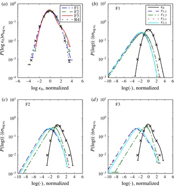
are shown in figure 8. The horizontal error bars, visible only for the smallest probability densities, are computed as described in the introduction to figure 1. The tabulated moments are given in table 5. For cases R4, F1 and F2, the lognormal distribution is a good model for
 ${\it\epsilon}_{0}$
at least within a few standard deviations of the mean. It may be that refined models being explored for isotropic turbulence, such as those reviewed by Donzis, Yeung & Sreenivasan (Reference Donzis, Yeung and Sreenivasan2008), more closely capture the behaviour at lower probability densities. Our interest, for now, is the behaviour near the mean, which is distinctly not lognormal for case F3, but rather tends towards bimodal. The bimodal tendency is also slightly apparent for case F2. It is not evident in case F1, but the positive skewness of case F1 relative to that of R4 is apparent in the figure.
(a) The p.d.f.s of the logarithm of
 ${\it\epsilon}_{0}$
, each normalised by its own mean and variance. (b–d) The p.d.f.s of the logarithm of
 ${\it\varepsilon}_{i,j}={\it\nu}(\partial u_{i}/\partial x_{j})^{2}$
, each normalised by the mean and variance of
 $\log {\it\epsilon}_{0}$
. The error bars indicate the range of values in each bin. The
 $\times$
symbols mark the standard Gaussian.

The skewness and kurtosis of the logarithms of
 ${\it\epsilon}_{0}$
and
 ${\it\chi}_{0}$
.

To understand the behaviour of
 $P(\log {\it\epsilon}_{0})$
, the distributions for the contributions to the dissipation rate
 ${\it\varepsilon}_{i,j}={\it\nu}(\partial u_{i}/\partial x_{j})^{2}$
are included in figure 8 for the stratified cases. Each curve is normalised by the mean and variance of
 $\log {\it\epsilon}_{0}$
so that the importance of the vertical shearing of the horizontal motion is not masked by the scaling. The curves for case R4 (not shown) are very similar to those for case F1 (cf. Almalkie & de Bruyn Kops Reference Almalkie and de Bruyn Kops2012a
, figure 7). The probability densities of the elements of
 ${\it\varepsilon}_{i,j}$
are distinctly not lognormal and, in fact, have left tails that appear to be exponential. Yet the lognormal model is a good approximation for the distribution of the sum of the nine elements in
 ${\it\varepsilon}_{i,j}$
in case F1. This characteristic is also observed for isotropic homogeneous turbulence (Almalkie & de Bruyn Kops Reference Almalkie and de Bruyn Kops2012a
), but the physical mechanism that causes this behaviour is an open question to the best of our knowledge. As
 $\mathit{Re}_{b}$
decreases, vertical shearing of horizontal motion becomes the dominant contribution to
 ${\it\epsilon}_{0}$
and the departure of
 $P(\log {\it\epsilon}_{0})$
from Gaussian becomes pronounced. For some flows, vertical shearing accounts for most of the dissipation rate (e.g. Praud, Fincham & Sommeria Reference Praud, Fincham and Sommeria2005), and Hebert & de Bruyn Kops (Reference Hebert and de Bruyn Kops2006b
) discuss the trend with
 $\mathit{Re}_{b}$
.
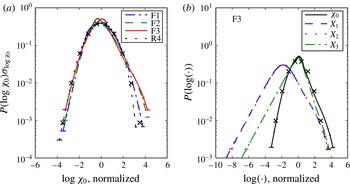
The p.d.f.s of
 $\log {\it\chi}_{0}$
are shown in figure 9 with a pair of plots analogous to those in figure 8. Starting with case R4 in figure 9(a), we note that the distribution is approximately lognormal except at high values of
 $\log {\it\chi}_{0}$
where the probability density is lower than predicted by the standard Gaussian having the same mean and standard deviation. This is what was found by Antonia & Sreenivasan (Reference Antonia and Sreenivasan1977), and it accounts for the slight negative skewness reported in table 5. The kurtosis is identical to that reported in Antonia & Sreenivasan (Reference Antonia and Sreenivasan1977). Therefore again we conclude that R4 is an accurate reference case.
(a) The p.d.f.s the logarithm of
 ${\it\chi}_{0}$
, each normalised by its own mean and variance. (b) The p.d.f.s of the logarithm of
 $X_{1}=2D(\partial {\it\phi}/\partial x_{1})^{2}$
, etc., for case F3; each is normalised by the mean and variance of
 $\log {\it\chi}_{0}$
. The error bars indicate the range of values in each bin. The
 $\times$
symbols mark the standard Gaussian.

Turning now to the stratified cases and referring to figure 9 and table 5, it is apparent that stratification results in greater occurrence of high values of
 ${\it\chi}_{0}$
relative to the mean, which is reflected in a positive skewness and kurtosis that increases with stronger stratification. For the most strongly stratified case, there is an inflection point in the right side of
 $P(\log {\it\chi}_{0})$
, although not as pronounced as that for
 $P(\log {\it\epsilon}_{0})$
. Its cause is revealed in figure 9(b), where the p.d.f.s of the logarithms of the contributions to
 ${\it\chi}_{0}$
are plotted. The magnitude of the vertical derivative of
 ${\it\phi}$
is much higher on average than that of the horizontal derivatives. It is also noted that the left tails of p.d.f.s of the components of
 $\log {\it\chi}_{0}$
are close to exponential, consistent with laboratory data for buoyancy-driven turbulence (Zhou & Xia Reference Zhou and Xia2010).
6. Internal intermittency
While KOC scaling has been the basis for many turbulence models and simulation techniques, the historical record shows that some of its shortcomings were noted even before the first hypotheses were published in 1941 (Monin & Yaglom Reference Monin and Yaglom1971). In particular, it was noted that
 ${\it\epsilon}_{0}$
is a random variable. Accordingly, Kolmogorov (Reference Kolmogorov1962) and Oboukhov (Reference Oboukhov1962) introduced the dissipation rate of kinetic energy averaged over a spherical volume with linear dimension
 $r$
, which we denote by
 ${\it\epsilon}_{r}$
. They assumed that
 ${\it\epsilon}_{r}$
is distributed lognormally with variance
 $$\begin{eqnarray}{\it\sigma}_{\log {\it\epsilon}_{r}}^{2}=A+{\it\mu}\log \frac{L}{r}\end{eqnarray}$$
provided that
 $r$
is small compared with some outer scale
 $L$
. The additive constant
 $A$
depends on the macro structure of the flow. Van Atta (Reference Van Atta1971) proposed analogous scaling for the scalar field:
 $$\begin{eqnarray}{\it\sigma}_{\log {\it\chi}_{r}}^{2}=A_{{\it\phi}}+{\it\mu}_{{\it\phi}}\log \frac{L_{{\it\phi}}}{r}.\end{eqnarray}$$
The constants
 ${\it\mu}$
and
 ${\it\mu}_{{\it\phi}}$
are called ‘intermittency exponents’ when
 $r$
is in the inertial range, although that term is used in various ways in the literature (Sreenivasan & Kailasnath Reference Sreenivasan and Kailasnath1993). We will evaluate them for the current data sets in § 6.1. Let us first consider the assumption that
 ${\it\epsilon}_{r}$
and
 ${\it\chi}_{r}$
have lognormal distributions.
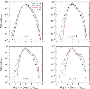
Normalised p.d.f.s of
 ${\it\epsilon}_{r}$
for several values of
 $r/{\it\lambda}$
. The black
 $\times$
symbols indicate the lognormal distribution.

In § 5 we conclude that
 ${\it\epsilon}_{0}$
and
 ${\it\chi}_{0}$
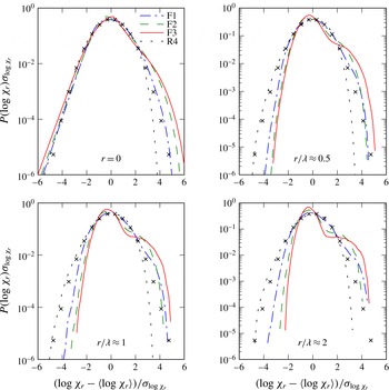
are well approximated by the lognormal assumption near their mean values provided that the buoyancy Reynolds number is high enough. Now let us see whether local averaging affects the applicability of the lognormal assumption. The p.d.f.s
 $P(\log {\it\epsilon}_{r})$
and
 $P(\log {\it\chi}_{r})$
are plotted in figures 10 and 11 respectively for several different values of
 $r/{\it\lambda}$
. Spherical averaging is performed using the method described in § 3.1. The upper left plot in each figure is for
 $r=0$
and so is of the same data discussed in § 5. As
 $r$
is increased, departure from lognormality becomes more pronounced, except for the unstratified case. This simply reflects the fact that the flows are more anisotropic at large scales than at small scales. Therefore averaging, a standard tool in turbulence modelling, will not obviate the need for a model for
 ${\it\epsilon}_{r}$
that is more sophisticated than the lognormal assumption, possibly such as those reviewed by Godeferd & Staquet (Reference Godeferd and Staquet2003).
Normalised p.d.f.s of
 ${\it\chi}_{r}$
for several values of
 $r/{\it\lambda}$
. The black
 $\times$
symbols indicate the lognormal distribution.

6.1. Intermittency exponents
While Kolmogorov and Oboukhov assumed the lognormal distribution expressed in (6.1) and (6.2), the theory of intermittency exponents was soon generalised so as not to require that assumption. In particular, Novikov & Stewart (Reference Novikov and Stewart1964) postulated that the second-order moment of
 ${\it\epsilon}_{r}$
has a universal form in the inertial range:
 $$\begin{eqnarray}\langle {\it\epsilon}_{r}^{2}\rangle \sim r^{-{\it\mu}}.\end{eqnarray}$$
Additional history on the topic is summarised by Sreenivasan & Kailasnath (Reference Sreenivasan and Kailasnath1993), who also consider several approaches for computing
 ${\it\mu}$
. Given the foregoing,
 ${\it\mu}$
and
 ${\it\mu}_{{\it\phi}}$
are of interest in stratified turbulence even though the lognormal assumption is not valid for the range of
 $\mathit{Re}_{b}$
we are considering.
The textbook value for
 ${\it\mu}$
with
 $r$
in the inertial range is
 ${\it\mu}\approx 0.25$
(Sreenivasan & Antonia Reference Sreenivasan and Antonia1997; Pope Reference Pope2000). Mydlarski & Warhaft (Reference Mydlarski and Warhaft1998) report
 ${\it\mu}_{{\it\phi}}\approx 0.2$
for grid turbulence at
 $\mathit{Re}_{{\it\lambda}}=100$
with a slight upward trend with increasing
 $\mathit{Re}_{{\it\lambda}}$
. Muschinski (Reference Muschinski2004) reports
 ${\it\mu}_{{\it\phi}}\approx 0.3$
in the stable nocturnal boundary layer. Sreenivasan & Kailasnath (Reference Sreenivasan and Kailasnath1993) suggest
 ${\it\mu}_{{\it\phi}}\approx 0.35$
based on Sreenivasan, Antonia & Danh (Reference Sreenivasan, Antonia and Danh1977) and Prasad, Meneveau & Sreenivasan (Reference Prasad, Meneveau and Sreenivasan1988). It should be noted that Almalkie & de Bruyn Kops (Reference Almalkie and de Bruyn Kops2012a
) report that
 ${\it\mu}$
computed from
 ${\it\epsilon}_{r}$
estimated from a single velocity derivative will be higher than
 ${\it\mu}$
computed from the true
 ${\it\epsilon}_{r}$
.
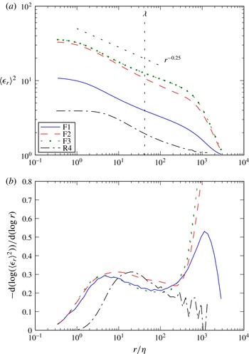
(a) The scale dependence of the second-order moments of
 ${\it\epsilon}_{r}$
. (b) The local scaling exponents. The Taylor microscale marked at
 $r/{\it\eta}=42$
is within
 $\pm 2$
of the true value for all cases (see table 1).

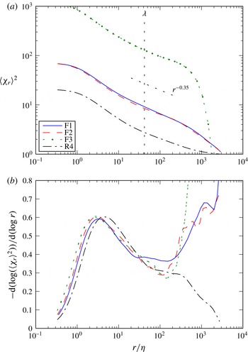
For the current data sets, the exponents are evaluated from the scale dependence of the variances of the filtered dissipation rates (cf. Sreenivasan & Kailasnath Reference Sreenivasan and Kailasnath1993), which are plotted as figures 12 and 13. Figures 12(a) and 13(a) show the variances of the locally averaged dissipation rates. Figures 12(b) and 13(b) are the local scaling exponents computed by taking the derivative of the data in figures 12(a) and 13(a). The local scaling exponent for
 $\langle {\it\epsilon}_{r}^{2}\rangle$
with
 $r$
in the inertial range is
 ${\it\mu}$
, and similarly for
 ${\it\mu}_{{\it\phi}}$
. The plots reveal no broad range of
 $r$
with power-law scaling, and the local scaling exponents decrease monotonically with increasing
 $r$
for
 $r$
in the vicinity of
 ${\it\lambda}$
. Similar behaviour is observed in high-Reynolds-number experimental measurements and atmospheric observations of Praskovsky & Oncley (Reference Praskovsky and Oncley1997) and so is presumably not an artefact of the limited dynamic range of the simulations. Since there is no broad range of
 $r$
where the local scaling exponent is constant, all we can conclude is that
 ${\it\mu}=0.25\pm 0.05$
and
 ${\it\mu}_{{\it\phi}}=0.35\pm 0.1$
in the vicinity of
 ${\it\lambda}$
, which is consistent with the published values cited at the beginning of this section.
(a) The scale dependence of the second-order moments of
 ${\it\chi}_{r}$
. (b) The local scaling exponents. The Taylor microscale marked at
 $r/{\it\eta}=42$
is within
 $\pm 2$
of the true value for all cases (see table 1).

7. Conclusions
The approach in this research is to simulate one of the simplest configurations for stratified turbulence at the highest dynamic range currently practicable and then to compare the results with those of an analogously simple unstratified flow in order to understand the applicability of classical scaling arguments to stratified turbulence. By this approach we can consider whether stratified turbulence is consistent with the classical arguments of Kolmogorov, Oboukhov and Corrsin (KOC) to the extent exhibited by unstratified turbulence given the limited dynamic range and finite sample size in the data sets. To implement this approach, stratified turbulence with three buoyancy Reynolds numbers is simulated on grids with up to
 $8192\times 8192\times 4096$
grid points and compared with isotropic homogeneous turbulence with a Taylor Reynolds number of 400 resolved on
 $8192^{3}$
grid points. It is concluded that the unstratified reference case is fully consistent with published simulation and laboratory results with regards to agreeing with KOC scaling and, therefore, is a useful reference case for stratified flows with the same dynamic range of horizontal length scales.
In § 1, it is observed that
 ${\it\eta}$
and
 $L_{o}$
are length scales dependent on
 $\{\langle {\it\epsilon}\rangle ,{\it\nu}\}$
and
 $\{\langle {\it\epsilon}\rangle ,N\}$
respectively, and the question is raised as to whether both can be relevant in a stratified flow at low
 $\mathit{Re}_{b}$
, that is, if the scale separation between the two is small. From the stratified simulations, it is concluded that
 ${\it\eta}$
is relevant in that it is the appropriate length scale for the kinetic energy dissipation scale, regardless of
 $\mathit{Re}_{b}$
. Not only do the second-order spectra and structure functions in the dissipation range collapse to a single curve independent of
 $\mathit{Re}_{b}$
, but the third-order structure functions coincide with theoretical relationships. The Kolmogorov length scale, which is equal to the Batchelor length scale in these simulations, very nearly collapses the scalar spectra and structure functions in the dissipation range, but the effects of stratification can be observed far into the dissipation range when
 $\mathit{Re}_{b}=13$
and 48. Therefore, the current data support the conclusion of Zhou & Xia (Reference Zhou and Xia2010) for buoyancy-driven turbulence that the dissipative scales are insensitive to large-scale inhomogeneity and anisotropy in the flow, although the current calculations are sensitive enough to detect the effects of stratification at all scales except for the case with
 $\mathit{Re}_{b}=220$
.
The second KOC similarity hypothesis is that turbulence statistics at length scales smaller than the outer scales and larger than the dissipative scales are universal and depend only on the dissipation rate. In the limit of
 $\mathit{Re}_{b}\rightarrow 1$
, there is no scale separation between the Ozmidov and Kolmogorov length scales for universal KOC statistics to develop. Of interest is whether KOC scaling holds for strongly stratified flows with
 $13\leqslant \mathit{Re}_{b}\leqslant 220$
. Based on spectra and structure functions, it is concluded that only the unstratified benchmark and the stratified case with
 $\mathit{Re}_{b}=220$
are consistent with KOC scaling. Even with
 $\mathit{Re}_{b}=220$
, deviation from KOC scaling can be seen in the third-order velocity structure function. At lower
 $\mathit{Re}_{b}$
, the
 $-5/3$
law for the spectra might appear to be applicable until one considers that the
 $-5/3$
slope occurs in the range of wavenumbers where the bottleneck effect is expected, that is, at the top of the dissipation range. There is no suggestion of KOC scaling in either the velocity or scalar structure functions for the simulations with
 $\mathit{Re}_{b}=13$
or 48, although the Yaglom relationship is satisfied.
In the original KOC hypotheses, the dissipation rates are taken to be constants over some volume of space. It has long been known that this is not the case, and so the distribution of the local, and locally averaged, dissipation rates is of interest. For
 $\mathit{Re}_{b}=48$
and 220, the distributions of
 ${\it\epsilon}_{0}$
and
 ${\it\chi}_{0}$
are only slightly different from that of the unstratified benchmark and so can be modelled with a lognormal distribution for many purposes. It should be noted that even in unstratified turbulence, that model is not good far from the mean. In particular, the right tail of
 $P({\it\chi}_{0})$
lies significantly below that of the lognormal model, which means that the model overpredicts the occurrence of strong mixing events. Stratification does not change this result. It is also observed that the p.d.f.s of the contributions to
 ${\it\epsilon}_{0}$
and
 ${\it\chi}_{0}$
are not much affected by stratification provided that
 $\mathit{Re}_{b}=48$
or higher. For the case with
 $\mathit{Re}_{b}=13$
, though, the lognormal model is poor for either
 $P({\it\epsilon}_{0})$
or
 $P({\it\chi}_{0})$
because the vertical gradients contribute significantly to the dissipation rates.
The refined similarity hypotheses of Kolmogorov and Oboukhov relate to the scaling of the locally averaged dissipation rates with the size of the averaging volume,
 $r$
. As with all published data of which we are aware, the current data show no broad range of
 $r$
with consistent power-law scaling. The intermittency exponents, though, evaluated in the vicinity of
 ${\it\lambda}$
for both the velocity and scalar are in the ranges of published values for all of the current simulations, and there is no apparent trend with
 $\mathit{Re}_{b}$
.
It is important to note that all of the conclusions from this research are for flows with equal diffusivities of momentum, heat and mass. Simply considering non-unity Schmidt number with no buoyancy effects is a significant complication (Yeung et al.
Reference Yeung, Xu and Sreenivasan2002). Nevertheless, the simple cases presented here provide some insight into whether KOC scaling is applicable to stratified turbulence. Specifically, while internal intermittency appears to be unaffected by stratification when
 $\mathit{Re}_{b}\geqslant 13$
,
 $\mathit{Re}_{b}>O(100)$
is required for the first and second KOC hypotheses to be satisfied. Even with
 $\mathit{Re}_{b}=220$
, one only need look to the third-order structure functions to see that KOC scaling is not satisfied as well as in unstratified flows with comparable dynamic range.
Acknowledgements
The author thanks Professors P. Diamessis and J. Riley for many valuable discussions on stratified flows, and Dr S. Almalkie for her thoughts on local isotropy. This work was funded by the Office of Naval Research via grant N00014-12-1-0583. High-performance computing resources were provided through the US Department of Defense High Performance Computing Modernization Program by the Army Engineer Research and Development Center and the Army Research Laboratory under Frontier Project FP-CFD-FY14-007.