1 Introduction
The variable-density jet is a canonical flow where the primary jet density differs from the ambient density. However, most studies have characterized its behaviour under fully turbulent flow. Lower Reynolds numbers (
 $Re$
), approaching transitional flow conditions in the near exit, add further complexity in terms of stability, where
 $Re$
represents the ratio of inertial to viscous forces. Transitional conditions exist at exit Reynolds numbers of approximately
 $10^{3}$
to
 $10^{4}$
. For a 10 cm diameter round jet, this range would exist at exit speeds of approximately 10 to
 $100~\text{cm}~\text{s}^{-1}$
in air, or 1 to
 $10~\text{cm}~\text{s}^{-1}$
in water. Such transitional and low turbulent jets can occur with smokestack emissions, impingement cooling and general flow control devices. In the natural world, examples include some submarine black smokers (Rona et al.
Reference Rona, Klinkhammer, Nelsen, Trefry and Elderfield1986; Ginster, Mottl & Von Herzen Reference Ginster, Mottl and Von Herzen1994), volcanic fumaroles (Sorey et al.
Reference Sorey, Kennedy, Evans, Farrar and Suemnicht1993; Stevenson Reference Stevenson1993) and rivulets or subaqueous springs that feed into lakes or streams. Volcanoes have much larger Reynolds numbers, since their vent diameters and exit speeds are considerably higher than the centimetre-scale dimensions above.
For many of these features, a key issue is entrainment. In volcanic regions, for example,
 $\text{CO}_{2}$
-bearing gas may exit from fumaroles, and it will either rise buoyantly or collapse gravitationally. This response depends on the exit velocity, temperature and entrainment rate into the exhausting flow. If there is collapse, the gas may pond in lethal concentrations. Along lake beds, sublacustrine springs bearing solutes may precipitate solids as the inflowing water entrains fluid of different temperature or chemical composition. Whether the solids disperse widely as fine particles or accumulate near the vent depends in part on the rate of near-vent entrainment. Results of the latter process include the spectacular, calcareous towers of tufa at Mono Lake, California (Dunn Reference Dunn1953).
Natural volcanic fumaroles, jets and plumes are commonly studied using one-dimensional models (Turner Reference Turner1986; Woods Reference Woods1993; Mastin Reference Mastin2007). These analyses typically use a constant entrainment ratio, based on a simple linear scaling between turbulent eddy velocity and jet centreline velocity (Morton, Taylor & Turner Reference Morton, Taylor and Turner1956). However, the entrainment ratio depends on a variety of parameters, including axial position (Falcone & Cataldo Reference Falcone and Cataldo2003), overpressure ratio (Solovitz, Mastin & Saffaraval Reference Solovitz, Mastin and Saffaraval2011), the ratio of the buoyant to inertial forces known as the Richardson number (
 $Ri$
) (Kaminski, Tait & Carazzo Reference Kaminski, Tait and Carazzo2005) and time (Chojnicki et al.
Reference Chojnicki, Clarke, Adrian and Phillips2014). There is also a Reynolds number dependence at lower values (Ricou & Spalding Reference Ricou and Spalding1961). In cases with cross-wind, the entrainment is also dependent on that velocity scale, with modelled values differing by an order of magnitude (Costa et al.
Reference Costa, Suzuki, Cerminara, Devenish, Esposti Ongaro, Herzog, Van Eaton, Denby, Bursik and de’Michieli Vitturi2016; Suzuki et al.
Reference Suzuki, Costa, Cerminara, Ongaro, Herzog, Van Eaton and Denby2016).
In geophysical systems, an obvious challenge is scaling, as many natural flows occur on scales larger than typical laboratory sizes. Hence, most existing studies match only some of the key non-dimensional parameters, and the results are rescaled. While many factors are important in eruptions, certainly critical are the exit diameter, speed and density relative to ambient. These variables can be expressed using the Reynolds and Richardson numbers, and sometimes also the density ratio of the jet to ambient. Springs, fumaroles and gas vents have a Reynolds number of the order of
 $10^{3}$
to
 $10^{7}$
, while volcanic eruptions can reach the order of
 $10^{9}$
(Sparks et al.
Reference Sparks, Bursik, Carey, Gilbert, Glaze, Sigurdsson and Woods1997). Most also have a small, but non-negligible Richardson number, with a magnitude of the order of 0.001 to 0.1 (Sparks Reference Sparks1986; Kaminski et al.
Reference Kaminski, Tait and Carazzo2005; Patrick Reference Patrick2007). Air experiments often reach the Reynolds number range, while liquid experiments typically consider the appropriate Richardson number range. Unfortunately, it is not common for both ranges to be met in the laboratory, and most of these cases consider only the self-similar region well downstream of the exit. There is limited information on the second-order moments, for cases where the buoyant exit flow transitions from laminar to turbulent, and even non-buoyant cases have only received limited attention in this range. Thus, there is an opportunity to explore entrainment response in this regime. The characteristics of variable-density jets are analysed with application to geophysical phenomena at
 $Re$
below
 $10^{4}$
and
 $Ri$
of the order of 0.001.
2 Background
A classic work is by Ricou & Spalding (Reference Ricou and Spalding1961), who measured the bulk entrainment into a variety of gases by balancing flows through a porous cylindrical wall. They consider a range of axial positions from the near exit,
 $x/D\sim 2$
, to far downstream in the self-similar region,
 $x/D\sim 400$
, where
 $x$
is the position and
 $D$
is the jet diameter. In the downstream region, the entrainment ratio was approximately constant for Reynolds numbers above
 $2.5\times 10^{4}$
, while it was more than 25 % higher at Reynolds numbers below
 $10^{4}$
. When comparing the response ranging from low-density hydrogen to higher-density propane and carbon dioxide, the entrainment ratio depended on the square root of the gas density. This dependence was explained from a control volume analysis, and it fit with the earlier scaling suggested by Thring & Newby (Reference Thring and Newby1953).
Several studies examined the finer details of variable-density jet flows, partly in the near-exit region (Kyle & Sreenivasan Reference Kyle and Sreenivasan1993) and partly far downstream (Panchapakesan & Lumley Reference Panchapakesan and Lumley1993). Kyle & Sreenivasan (Reference Kyle and Sreenivasan1993) considered helium/air mixtures ejected at Reynolds numbers from 2100 to 16 000, and high-speed photography displayed the formation of axisymmetric vortex ring instabilities. Hot-wire anemometry demonstrated how oscillating modes depended on flow conditions. Some of these instabilities were comparable to observations of heated air jets (Monkewitz et al.
Reference Monkewitz, Lehmann, Barsikow and Bechert1989). Panchapakesan & Lumley (Reference Panchapakesan and Lumley1993) used piggy-backed concentration and cross-wire probes to examine turbulent statistics and budgets for a helium jet exhausting into air. When compared to air jets, axial velocity fluctuations were significantly higher with helium, yet radial fluctuations were similar. They suggest the difference may be due to near-field effects, though their tests were conducted with
 $x/D>50$
.
Soon afterward, an extensive laser Doppler velocimetry (LDV) study considered the turbulence development in a variable-density jet exhausting into a weak co-flow (Gharbi, Amielh & Anselmet Reference Gharbi, Amielh and Anselmet1995; Amielh et al.
Reference Amielh, Djeridane, Anselmet and Fulachier1996; Djeridane et al.
Reference Djeridane, Amielh, Anselmet and Fulachier1996). Gharbi et al. (Reference Gharbi, Amielh and Anselmet1995) examined the near-exit region, from
 $x/D\sim 0.2$
to 30, with gases including low-density helium and higher-density carbon dioxide. All cases had the same exit momentum flux, which resulted in
 $Re$
of 7000 and larger. With the helium jet, the turbulence development was rapid, with both axial and radial fluctuations reaching a constant level by
 $x/D\sim 6$
. Djeridane et al. (Reference Djeridane, Amielh, Anselmet and Fulachier1996) continued the study, demonstrating higher volumetric entrainment with lower-density fluid. They also found more rapid growth of turbulent kinetic energy and third-order moments, which they suggest was due to larger vortices at lower density.
Amielh et al. (Reference Amielh, Djeridane, Anselmet and Fulachier1996) demonstrated through experiments that low-density gases approach the fully developed response shown by Panchapakesan & Lumley (Reference Panchapakesan and Lumley1993) much more rapidly than higher-density air or carbon dioxide. More recently, Wang et al. (Reference Wang, Fröhlich, Michelassi and Rodi2008) conducted large-eddy simulations of the Amielh et al. (Reference Amielh, Djeridane, Anselmet and Fulachier1996) geometry, and these matched the experiments quite well. These simulations also displayed the three-dimensional development of vortex instabilities, showing more significant streamwise vorticity at lower density.
Although particle image velocimetry (PIV) has been commonly used, there has been very limited study of turbulence development of variable-density jets. Recker et al. (Reference Recker, Wagemakers, Janssens and Gilson2012) recently used PIV for a series of experiments with both heated air and helium/air mixtures. They examined locations from the near exit to the fully developed region, considering jet-to-ambient density ratios down to 0.3 and Reynolds numbers below 10 000. Axial development of centreline speed and half-width match with earlier results (Chen & Rodi Reference Chen and Rodi1980), but the details of the turbulence were only qualitatively considered. Variable-density jet studies by Papanicolaou & List (Reference Papanicolaou and List1988) and Wang & Law (Reference Wang and Law2002) also used non-intrusive methods, though each focused primarily on axial locations well downstream of the developing region.
Gerashchenko & Prestridge (Reference Gerashchenko and Prestridge2015) investigated variable-density mixing of miscible gases using PIV and planar laser-induced fluorescence. Near- and far-field measurements were performed to compare effects of high and low Atwood numbers, representing the density ratio of the two fluids,
 $(\unicode[STIX]{x1D70C}_{1}-\unicode[STIX]{x1D70C}_{2})/(\unicode[STIX]{x1D70C}_{1}+\unicode[STIX]{x1D70C}_{2})$
, where
 $\unicode[STIX]{x1D70C}_{1}$
is the heavier fluid. It was found that slower mixing is demonstrated by high Atwood number jets. Density gradients impacted turbulent kinetic energy of the flow significantly, increasing the magnitude by fourfold at the downstream location of
 $x/D=14$
. Within the near-jet region,
 $x/D<4$
, density effects were minimal in comparison to furthest downstream locations.
While there has been limited quantitative study of Reynolds number effects in variable-density jet turbulence, neutrally buoyant cases have been examined over a wider range of conditions. This includes lower Reynolds numbers, even down to laminar exit flows. O’Neill, Soria & Honnery (Reference O’Neill, Soria and Honnery2004) used PIV to analyse water jets in water at Reynolds numbers of approximately 700 and 1000, considering two axial regions near the exit and farther downstream. At the lower
 $Re$
, the jet appears to be stable and laminar, with very low turbulent stresses. At the higher level, the jet is more turbulent, and turbulent stresses are near the expected self-similar magnitudes. Surprisingly, flow visualization contrasted with the PIV measurements, showing the Kelvin–Helmholtz instability and clear oscillations for both Reynolds numbers tested.
Kwon & Seo (Reference Kwon and Seo2005) conducted a thorough PIV study of non-buoyant jets exhausting from a contraction nozzle, with Reynolds numbers ranging from approximately 200 to 5000. All flows exited with a top-hat profile, and in most cases diffused out to a Gaussian profile within the first 20 diameters. At low
 $Re$
, though, the jet remained relatively stable, retaining the top-hat profile more than 40 diameters downstream of the exit. High
 $Re$
jets had shorter development lengths, and they had higher turbulence intensities near the exit. However, the spatial resolution in this study was somewhat limited, with only approximately 5 data points across the jet diameter at the exit.
The plane jet is a related geometry, as it features mixing layers between the central core flow and the ambient. Kotsovinos (Reference Kotsovinos1976) considered the spreading rate of these jets, demonstrating a nonlinear response. Namer & Ötügen (Reference Namer and Ötügen1988) used hot-wire anemometry and laser Doppler anemometry to examine plane jets at Reynolds numbers below 7000, and they observed decreased eddy sizes at higher
 $Re$
. This led to a reduction in mixing and the corresponding spreading rate. Suresh et al. (Reference Suresh, Srinivasan, Sundararajan and Das2008) specifically focused on plane jets in the transitional regime, using hot-wire anemometry for
 $Re$
between 250 and 6250. In the near field, they observed little decay of the centreline velocity at low
 $Re$
, and the turbulent intensity was substantially reduced for these same cases. They also noted that the near-field region is dominated by vortex shedding due to shear layer instability. Quite recently, Paillat & Kaminski (Reference Paillat and Kaminski2014) specifically considered entrainment into planar jets due to their importance in geophysical phenomena, although they examined relatively low Reynolds numbers between approximately 50 and 450. Using PIV measurements well downstream of the exit, they found that the entrainment ratio had some variation with Reynolds number, which they attributed to the evolution of the Reynolds shear stresses. It is worth noting that none of these plane jets had densities differing from the ambient.
Turbulence of a jet can be characterized by the utilization of numerous analytic methods. The entrainment of jet flow, specifically, can be obtained from quadrant analysis (Wallace Reference Wallace2016). This analysis technique fragments fluctuating velocity components into four events, from which entrainment can be visualized and quantified and its dependent parameters can be investigated. The Reynolds shear stress obtained by this technique can also be used in closure modelling (Katul et al. Reference Katul, Poggi, Cava and Finnigan2006; Poggi & Katul Reference Poggi and Katul2007). With the closure model, flow characteristics can be obtained from mathematical equations of the flow that are too complicated to be solved numerically. This technique can be utilized to advance predictive modelling of geophysical flows. Quadrant analysis has rarely been applied to free shear jet flow. For this reason, wall-bounded jet flow studies must be investigated to gain an understanding of previous research and advances in the technique.
Sreenivasan & Antonia (Reference Sreenivasan and Antonia1978) studied joint probability density functions and quadrant analysis of a heated jet with a co-flowing external stream. The study identified the most significant departures from Gaussian behaviour occurred in quadrants (
 $x,y<0$
) and (
 $x,y>0$
) in the intermittent region, with large contributions to
 $\langle xy\rangle$
, where
 $x,y$
refer to the streamwise and spanwise velocity fluctuations as well as temperature fluctuations. Yoon & Lee (Reference Yoon and Lee2003) investigated the entrainment rate of an elliptic jet via mean velocity fields. The study found the jet width growth was faster along the minor axis and subsequently the entrainment of surrounding fluid was more active on the minor axis when compared with the major axis. Krug et al. (Reference Krug, Chung, Philip and Marusic2017) explored the role of buoyancy on the entrainment by studying simulated temporal plume development. Analysis showed that the buoyancy contribution accounts for
 ${\sim}15\,\%$
of the magnitude of the entrainment coefficient.
Jet studies with the application of quadrant analysis include studies of the mixing characteristics of a swirling and non-swirling jet from a fully developed rotating pipe flow (Örlü & Alfredsson Reference Örlü and Alfredsson2008) as well as turbulent wall jets (Nolan, Walsh & McEligot Reference Nolan, Walsh and McEligot2010). Örlü & Alfredsson (Reference Örlü and Alfredsson2008) found that the swirling jet spreads, mixes and evolves faster when compared to the non-swirling counterpart. The shortened distance and therefore time needed to mix the jet and the ambient air in the swirling jet case also indicate a high correlation between fluctuations in streamwise velocity and temperature. Nolan et al. (Reference Nolan, Walsh and McEligot2010) used quadrant analysis of PIV data to isolate contributors to the Reynolds shear stresses to identify energetic structures within the flow responsible for turbulent kinetic energy production. It was found that ‘ejection’ events, Q2, exhibit the largest growth at the boundary-layer edge, indicating large-scale disturbances at that region, whereas ‘sweep’ events, Q4, are large close to the wall with increased Reynolds number and intermittency.
Additionally, turbulence development can be characterized by utilizing proper orthogonal decomposition (POD), an analysis technique used to extract a set of basis functions and organize the functions according to energy content. This allows for the derivation of low-dimensional descriptions of dynamical systems that act as a mathematical representation of the flow field. This set of functions can be used to create a low-order description of the variable-density jet, simplifying the geophysical flow model for further analysis.
POD has been employed in previous jet studies to gain a better understanding of velocity fluctuations in recirculation zones of an annular jet. These jets are typically used in industrial combustion and treatment processes. Patte-Rouland et al. (Reference Patte-Rouland, Lalizel, Moreau and Rouland2001) used PIV to characterize spatial velocity oscillations, and POD was implemented to dissociate the oscillation and velocity fluctuations from turbulent behaviour. Berkooz, Holmes & Lumley (Reference Berkooz, Holmes and Lumley1993) used POD to analyse a turbulent jet in cross-flow, which is a common way to mix two fluids. POD analysis showed that wake vortices caused a strong interaction between the jet core and cross-flow. Arndt, Long & Glauser (Reference Arndt, Long and Glauser1997) used POD to study the pressure field fluctuations surrounding a turbulent jet. Using the results, the characteristic signal form was reconstructed to show that vortex pairing is random in both time and space, even at low Reynolds numbers.
Because of the opportunities listed above, a series of experiments was performed to examine the flow response in the near-exit region of a variable-density jet. Particle image velocimetry was employed to investigate the instantaneous and ensemble-averaged response of air, argon and helium jets ejecting vertically from a long pipe into ambient air. Exit Reynolds numbers ranged from approximately 1500 to 10 000, encompassing laminar to turbulent exit conditions. The analysis focused on the entrainment, turbulent Reynolds stresses and flow structures, demonstrating the modification of mixing mechanisms about the transition point. These latter issues are discussed in context of both natural and relevant engineering flows.
3 Theory
A jet or plume is a representation of a turbulent free shear flow. Including external forces such as gravity, a momentum transport equation is defined as
 $$\begin{eqnarray}U\frac{\unicode[STIX]{x2202}U}{\unicode[STIX]{x2202}x}+V\frac{\unicode[STIX]{x2202}U}{\unicode[STIX]{x2202}y}=-\frac{1}{\unicode[STIX]{x1D70C}}\frac{\unicode[STIX]{x2202}P}{\unicode[STIX]{x2202}x}+\unicode[STIX]{x1D708}\frac{\unicode[STIX]{x2202}^{2}U}{\unicode[STIX]{x2202}x^{2}}+\unicode[STIX]{x1D708}\frac{\unicode[STIX]{x2202}^{2}U}{\unicode[STIX]{x2202}y^{2}}-\frac{\unicode[STIX]{x2202}\langle u^{2}\rangle }{\unicode[STIX]{x2202}x}-\frac{\unicode[STIX]{x2202}\langle uv\rangle }{\unicode[STIX]{x2202}y}+f_{x},\end{eqnarray}$$
where
 $\unicode[STIX]{x1D70C}$
is density of the jet,
 $P$
is the pressure,
 $\unicode[STIX]{x1D708}$
is the kinematic viscosity of the jet,
 $U$
and
 $V$
are the respective streamwise and spanwise mean velocity components and
 $u$
and
 $v$
are the corresponding fluctuating velocity components (Pope Reference Pope2000). Here,
 $f_{x}$
, the force due to gravity per mass, is also included due to buoyancy effects. The
 $\langle \cdot \rangle$
denotes ensemble averaging. These yield the in-plane Reynolds shear stress component,
 $\langle uv\rangle$
(Tennekes & Lumley Reference Tennekes and Lumley1972). In free shear flows, change in pressure and viscous transport of momentum are negligible, therefore the first three terms on the right-hand side of the equation can be neglected. For the vertically oriented jet, the streamwise velocity corresponds to the vertical direction of the jet, and transverse velocity is in the horizontal direction as seen in figure 1.
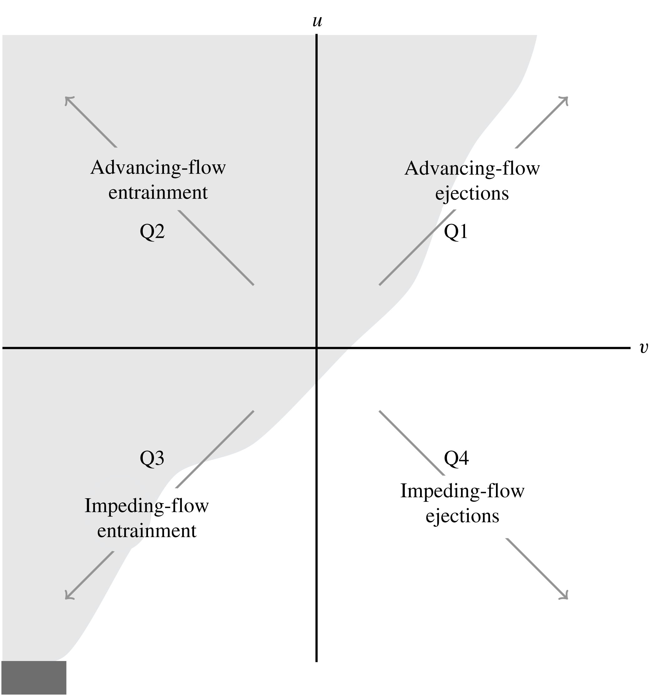
Four quadrants shown where
 $u$
and
 $v$
are the streamwise and spanwise velocity fluctuations, respectively. New terminology is introduced for Q1 to Q4 to describe the vertically oriented free shear jet.

3.1 Quadrant analysis
Quadrant analysis is used to characterize and classify events per the Reynolds stress, utilizing conditional averaging to break up the signal of fluctuating velocity components into four events or quadrants based on the sign of the in-plane components. The conditional average of the Reynolds shear stress computed using quadrant analysis is defined as
 $$\begin{eqnarray}\langle uv\rangle =\frac{1}{N}\mathop{\sum }_{n=1}^{N}u_{n}(x,y)v_{n}(x,y)I_{m}[u_{n}(x,y);v_{n}(x,y)],\end{eqnarray}$$
where
 $m$
represents the quadrant (i.e.
 $m=1,2,3,4$
),
 $n$
is the signal for a given snapshot and
 $N$
is the total number of snapshots.
 $I_{m}$
is the indicator function that takes a unit value when
 $u$
and
 $v$
are in quadrant
 $m$
and is defined as
 $$\begin{eqnarray}I_{m}[u_{n}(x,y);v_{n}(x,y)]=\left\{\begin{array}{@{}ll@{}}1,\quad & \text{if }(u_{n},v_{n})\text{ is in quadrant }m\\ 0,\quad & \text{otherwise}.\end{array}\right.\end{eqnarray}$$
The imbalance of quadrants is referred to as
 $$\begin{eqnarray}\unicode[STIX]{x0394}Q_{\unicode[STIX]{x1D6FC}\unicode[STIX]{x1D6FD}}=Q_{\unicode[STIX]{x1D6FC}}-Q_{\unicode[STIX]{x1D6FD}}.\end{eqnarray}$$
where
 $\unicode[STIX]{x1D6FC},\unicode[STIX]{x1D6FD}=1,2,3,4$
. This quantity shows which quadrant contributes the most shear stresses in relation to the streamwise and spanwise location of the developing jet. A similar application was used by Raupach (Reference Raupach1981) who studied the difference between sweeps and ejections, Q2 and Q4, in smooth and rough wall turbulent boundary layers based on the stress fraction quantity,
 $\unicode[STIX]{x0394}S_{m}$
. The stress fraction is the relative contribution of stress from each quadrant to the overall stress contribution and is expressed as
 $\unicode[STIX]{x0394}S_{m}=\langle uv\rangle _{m}/\langle uv\rangle$
.
In past studies of wall-bounded jets, the four quadrants have previously been defined as Q1: outward interactions (
 $u>0$
and
 $v>0$
), Q2: ejections (
 $u>0$
and
 $v<0$
), Q3: inward interactions (
 $u<0$
and
 $v<0$
) and Q4: sweeps (
 $u<0$
and
 $v>0$
). These quadrants exist on a Cartesian plane whose abscissa is
 $u$
and ordinate is
 $v$
. In wall-bounded flow, fluctuations are often anti-correlated,
 $-\langle uv\rangle >0$
, and Q2 and Q4, ejections and sweeps, are typically the largest contributors to overall Reynolds stress (Raupach Reference Raupach1981; Hamilton et al.
Reference Hamilton, Kang, Meneveau and Cal2012). In wall-bounded flow studies, ejections are upward turbulent bursts with velocities slower than the mean, while sweeps are downward turbulent bursts in the positive streamwise direction (Hamilton et al.
Reference Hamilton, Kang, Meneveau and Cal2012). For a comprehensive history of quadrant analysis, refer to Wallace (Reference Wallace2016).
For a vertically oriented open jet, new terminology is introduced to align and correctly describe the flow characteristics, where Q1 to Q4 are herein referred to as advancing-flow ejections, advancing-flow entrainment, impeding-flow entrainment and impeding-flow ejections, respectively. It is of note that the jet is quasi-symmetric and therefore the new terminology and analysis are only applicable to one half of the jet. The right side of the jet is chosen for the introduced nomenclature and is utilized in the following results of quadrant analysis for this study. The coordinates are also reoriented, shown in figure 1, where the abscissa is
 $v$
and ordinate is
 $u$
on a Cartesian plane. Using quadrant analysis of Reynolds shear stress, entrainment of the flow is further explained through the shear layer as the jet develops downstream. Entrainment along the edge and in the mixing layer of the right side of the jet can be characterized using Q2 and Q3. Entrainment is dictated by the sign of the spanwise fluctuations, identified by direction of the velocity fluctuation pointing towards the centre of the jet.
3.2 Proper orthogonal decomposition
Classical POD was introduced to fluid mechanics by Lumley (Reference Lumley1967), applying the analysis technique to turbulent velocity signals. The method of snapshots, first introduced by Sirovich (Reference Sirovich1987), is implemented when the flow measurements contain high spatial resolution in comparison to temporal resolution. Therefore, snapshot POD is applied to the variable-density jet due to the high spatial characteristics associated with PIV measurements. Further discussion of classical POD theory is omitted from this section.
For snapshot POD, a spatial correlation matrix is used to compute eigenfunctions and consequently decorrelate structures contained in the snapshots. The two-point spatial correlation tensor,
 $\unicode[STIX]{x1D64D}(\boldsymbol{x},\boldsymbol{x}^{\prime })$
, is defined as
 $$\begin{eqnarray}\unicode[STIX]{x1D64D}(\boldsymbol{x},\boldsymbol{x}^{\prime })=\frac{1}{N}\mathop{\sum }_{n=1}^{N}\boldsymbol{u}(\boldsymbol{x},t^{n})\boldsymbol{u}^{T}(\boldsymbol{x}^{\prime },t^{n}),\end{eqnarray}$$
where
 $u(\boldsymbol{x},t^{n})$
is the stochastic flow field,
 $t^{n}$
is the time at a sample
 $n$
,
 $N$
refers to the number of snapshots and the prime represents the spatial coordinate of another point in the domain. The bold symbols represent vector arrays.
Assuming the basis modes can be written in terms of the original data and a coefficient
 $A$
, then the deterministic field,
 $$\begin{eqnarray}\unicode[STIX]{x1D731}(\boldsymbol{x})=\mathop{\sum }_{n=1}^{N}A(t^{n})\boldsymbol{u}(\boldsymbol{x},t^{n}),\end{eqnarray}$$
has the largest projection on the stochastic velocity field, indicating the correlation tensor, equation (3.5), becomes the kernel of the POD. The POD integral equation is defined as the solution to the Euler–Lagrange integral equation,
 $$\begin{eqnarray}\int _{\unicode[STIX]{x1D6FA}}\unicode[STIX]{x1D64D}(\boldsymbol{x},\boldsymbol{x}^{\prime })\unicode[STIX]{x1D731}^{i}(\boldsymbol{x}^{\prime })\,\text{d}\boldsymbol{x}^{\prime }=\unicode[STIX]{x1D706}^{i}\unicode[STIX]{x1D731}^{i}(\boldsymbol{x}).\end{eqnarray}$$
The solution of (3.7) yields a complete set of orthogonal eigenfunctions. Substitution of the combinations of equations (3.5) and (3.6) into the Euler–Lagrange integral equation and the discretization of quantities results in an eigenvalue problem described as
 $$\begin{eqnarray}\unicode[STIX]{x1D63E}\boldsymbol{A}=\unicode[STIX]{x1D740}\boldsymbol{A},\end{eqnarray}$$
where
 $\unicode[STIX]{x1D63E}$
is a symmetric
 $N\times N$
matrix with components
 $\unicode[STIX]{x1D60A}_{jk}=(1/N)(\boldsymbol{u}^{T}(\boldsymbol{x},t^{j})\boldsymbol{u}(\boldsymbol{x},t^{k}))$
, where
 $j,k=1,\ldots ,N$
. The coefficient vector,
 $\boldsymbol{A}$
, is defined as
 $[A(t^{1}),A(t^{2}),\ldots ,A(t^{n})]^{\text{T}}$
and
 $\unicode[STIX]{x1D740}$
is a diagonal matrix of
 $N$
eigenvalues. The eigenvalues and associated eigenmodes are ordered by their contribution of energy,
 $\unicode[STIX]{x1D706}^{1}>\unicode[STIX]{x1D706}^{2}>\unicode[STIX]{x1D706}^{3}>\cdots >\unicode[STIX]{x1D706}^{n}$
.
The set of coefficients from which the POD modes are computed, according to the eigenvalue problem, are obtained from the solution of equation (3.8). The modes are normalized and formed into an orthonormal basis defined as
 $$\begin{eqnarray}\unicode[STIX]{x1D731}^{i}(\boldsymbol{x})=\frac{\displaystyle \mathop{\sum }_{n=1}^{N}A^{i}(t^{n})\boldsymbol{u}(\boldsymbol{x},t^{n})}{\left\Vert \displaystyle \mathop{\sum }_{n=1}^{N}A^{i}(t^{n})\boldsymbol{u}(\boldsymbol{x},t^{n})\right\Vert },\quad i=1,2,\ldots .\end{eqnarray}$$
Using the eigenfunctions of the POD, velocity fluctuations may be reconstructed, and as a result, the Reynolds stresses are reconstructed as
 $$\begin{eqnarray}\langle u_{i}(\boldsymbol{x})u_{j}(\boldsymbol{x})\rangle =\left\langle \mathop{\sum }_{n=1}^{N}a_{n}^{2}\unicode[STIX]{x1D6F7}_{i}^{n}(\boldsymbol{x})\unicode[STIX]{x1D6F7}_{j}^{n}(\boldsymbol{x})\right\rangle .\end{eqnarray}$$
The set of coefficients,
 $a_{n}$
, yielded by back projecting the stochastic velocity fields onto the deterministic POD modes, is defined as
 $$\begin{eqnarray}a_{n}=\int _{\unicode[STIX]{x1D6FA}}\boldsymbol{u}(\boldsymbol{x},t^{n})\unicode[STIX]{x1D731}^{n}(\boldsymbol{x})\,\text{d}\boldsymbol{x}^{\prime },\end{eqnarray}$$
in the domain
 $\unicode[STIX]{x1D6FA}$
.
A set of eigenfunctions that represent the modes of turbulence and eigenvalues that measure the energy associated with each eigenfunction are provided from the POD analysis. The total turbulence kinetic energy,
 $$\begin{eqnarray}E=\frac{1}{2}\int _{\unicode[STIX]{x1D6FA}}(\overline{\boldsymbol{u}\boldsymbol{u}}+\overline{\boldsymbol{v}\boldsymbol{v}})=\mathop{\sum }_{n=1}^{N}\unicode[STIX]{x1D706}_{n},\end{eqnarray}$$
equals the summation of the eigenvalues and is obtained by reducing
 $\unicode[STIX]{x1D619}_{ij}(\boldsymbol{x},\boldsymbol{x}^{\prime })$
.
4 Experimental methods
4.1 Jet flow apparatus
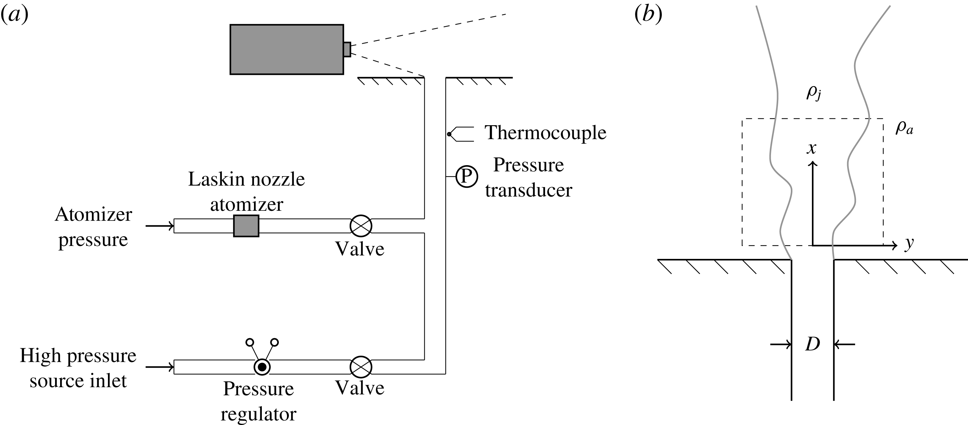
The experiments used a vertical pipe apparatus, shown in figure 2, which is a modified version of a facility described in detail in Solovitz et al. (Reference Solovitz, Mastin and Saffaraval2011). Here, a compressed gas source is fed into the structure, where it is regulated and directed vertically out of a 305 mm long, constant-diameter pipe. In these experiments, the apparatus is fed with either compressed helium, air or argon, supplied by an external tank. The pipe exits normally from the centre of a 91.4 by 91.4 cm square, horizontal plate. The apparatus is placed on the floor in the centre of a laboratory approximately 10 by 10 by 10 m in size, and the jet exit is hundreds of diameters away from any wall.
The exit diameter of the jet is 11.84 mm, resulting in a non-dimensional pipe length of 26, exceeding classic criteria for fully developed turbulent flow (Kays & Crawford Reference Kays and Crawford1993). For turbulent conditions, the profile is comparable to the expected log law profile, but does have quantitative differences. For laminar conditions, the profile is nearly parabolic, indicating that this flow is approaching fully developed conditions as well. Static pressure and temperature are measured just upstream of the exit using a gage pressure transducer and T-type thermocouple, respectively. Minor corrections based on Fanno flow are made to these readings to determine the exit conditions.
Schematic of experimental apparatus, adapted from an earlier system developed by Solovitz et al. (Reference Solovitz, Mastin and Saffaraval2011).

Besides the primary flow line, there is a second feed pipe used for PIV seeding. This structure is fed by a second, regulated compressed gas tank, which charges a Laskin nozzle atomizer containing olive oil. This produces
 $1~\unicode[STIX]{x03BC}\text{m}$
oil droplets, which are carried with the gas into the primary flow. The seeder line tees into the apparatus well upstream of the final length of pipe, permitting the fluid to mix with the primary line. Although the seeder line could have served as the sole gas source, this dual-source design permits significantly higher exit speeds. Using standard tanks, a constant exit speed is produced for several minutes, which is sufficient to acquire steady-state measurements.
Since the olive oil tracers are only present in the jet itself, an additional fog generator provides seeding for the remainder of the ambient air. Prior to each experiment, this unit produces micron-scale droplets of aqueous glycol, which spread throughout the laboratory. Several minutes are allowed for the tracers to achieve a uniform distribution in the region near the jet exit, with background speeds typically less than
 $1~\text{mm}~\text{s}^{-1}$
. The density of olive oil and glycol tracers is similar in the collected PIV images.
4.2 PIV system
Data are acquired with a commercial PIV system. A dual-head laser emits a pair of closely timed pulses, each with 50 mJ energy and 532 nm wavelength. The pulses pass through a diverging cylindrical lens and a converging spherical lens, producing a laser sheet of approximately 0.5 mm thickness at the focal point. The sheet is aligned along the centreline of the jet, located in a vertical plane. The laser illuminates the embedded tracers, and their instantaneous distribution is captured using a 1.4-megapixel digital camera positioned perpendicular to the laser sheet. The laser and camera timing are controlled using a synchronizer, with the pulse timing selected to produce optimal accuracy for PIV analysis (Raffel, Willert & Kompenhans Reference Raffel, Willert and Kompenhans2013). Because of the significant variation in speeds between the jet and the entrained ambient, tests are performed at two different time delays to accurately capture the response in each region. Along the centreline, the pulses are spaced approximately
 $10~\unicode[STIX]{x03BC}\text{s}$
apart. In the ambient, the spacing is approximately
 $200~\unicode[STIX]{x03BC}\text{s}$
.
All PIV images are processed using Pivlab2000, an iterative code which determines the instantaneous, two-dimensional velocity field (Han Reference Han2001). This tool divides each image into smaller interrogation windows, which are cross-correlated to determine the pixel displacement in each region. In subsequent iterations, the windows are decreased in size, resulting in a high-resolution estimate of the tracer velocity. For the experiments here, the smallest region is 32 pixels by 32 pixels. Using a 50 % overlap, the physical dimension is 0.9
 $\times$
0.9 mm, resulting in more than 13 vectors across the jet exit profile and approximately 49 vectors in the streamwise direction.
Based on estimates for particle displacement error, time resolution, and calibration factors, the overall velocity uncertainty in the jet is
 $\pm$
2.0 % of the centreline speed. The turbulent fluctuation velocity has an uncertainty of
 $\pm$
8.0 % of the peak axial fluctuations. In the entrained region, the instantaneous velocity uncertainty is higher, at
 $\pm$
3.9 %, and the uncertainty in entrainment ratio is estimated at
 $\pm$
4.4 %. Parameters based on velocity gradients, such as vorticity and swirling strength, have an estimated uncertainty of
 $\pm$
13 %.
4.3 Test conditions
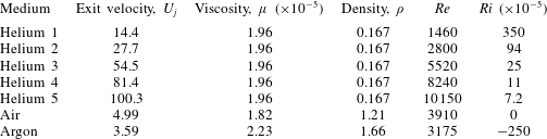
Seven test conditions were considered, with five using helium. In later discussion, these five cases are denoted helium 1 to 5. These buoyant cases spanned exit conditions from almost laminar to fully developed turbulent pipe flow. The only variable modified in the buoyant experiments was the exit velocity, resulting in a range of Reynolds and Richardson numbers. Here, the Reynolds number is
 $Re=\unicode[STIX]{x1D70C}_{j}U_{j}D/\unicode[STIX]{x1D707}_{j}$
, where
 $\unicode[STIX]{x1D70C}_{j}$
is the jet density,
 $U_{j}$
is the exit velocity,
 $D$
is the exit diameter and
 $\unicode[STIX]{x1D707}_{j}$
is the jet viscosity. The Richardson number, the inverse square of the Froude number, is
 $Ri=g(\unicode[STIX]{x1D70C}_{a}-\unicode[STIX]{x1D70C}_{j})D/(\unicode[STIX]{x1D70C}_{j}U_{j}^{2})$
, where
 $g$
is the gravitational acceleration and
 $\unicode[STIX]{x1D70C}_{a}=1.21~\text{kg}~\text{m}^{-3}$
is the ambient air density. Note that
 $Ri$
is sometimes defined with the reverse sign, but the form here is selected for consistency with earlier variable-density jet studies. The air and argon cases are selected because their Reynolds numbers are in the intermediate range between helium 1 and 3. For air, argon and helium, the density ratio between the jet and the ambient,
 $\unicode[STIX]{x1D70C}_{j}/\unicode[STIX]{x1D70C}_{a}$
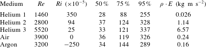
, is 1, 1.37 and 0.14. Table 1 shows the details of the test parameters.
Experimental test conditions.
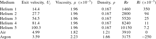
The Reynolds numbers are low enough that some exit conditions may be laminar, but most are turbulent at the exit. Even the lowest Reynolds number case is likely to transition farther downstream, leading to a turbulent jet flow. Although six of the seven test cases are positively or negatively buoyant, all of the flows are primarily dominated by inertia in the near-exit region, as defined using the jet length,
 $L_{jet}=M^{3/4}B^{-1/2}$
(Fischer et al.
Reference Fischer, List, Koh, Imberger and Brooks1979). Here,
 $M$
is the exit specific momentum flux and
 $B$
is the exit specific buoyancy flux. Using a simplified top-hat profile,
 $M=\unicode[STIX]{x03C0}D^{2}U^{2}/4$
and
 $B=\unicode[STIX]{x03C0}gD^{2}U\unicode[STIX]{x0394}\unicode[STIX]{x1D70C}/(4\unicode[STIX]{x1D70C}_{j})$
, resulting in a jet length
 $L_{jet}\approx D\cdot |Ri|^{-1/2}$
when neglecting a constant near unity. For the five positively buoyant cases, the corresponding jet length is greater than 16 diameters, which is well beyond the test region. For the negatively buoyant argon test case,
 $L_{jet}$
is approximately
 $19D$
. Hence, although there are density differences here, the flow is dominated by inertial effects. Still, this can have a significant impact, since an increase or decrease of jet inertia should influence the entrainment. Also, although the magnitudes of Richardson number are small, these levels occur in many natural or engineered flows.
The PIV images captured the first four diameters downstream of the exit, which is enough to examine the development region for helium at turbulent conditions. For each experiment, a total of 1000 PIV image pairs were captured – 500 focused on the jet, and 500 focused on the entrained ambient flow. Although these latter data are used for examining the entrainment, the measured ambient velocities agree with the former series to within 10 %, even though the timing is not optimized in that region. Several of these experiments were repeated to validate the results, and the measurements were consistent to within the uncertainty.
5 Results
The variable-density jets are studied via several methods, extracting information from the full-field PIV measurements. First, instantaneous flow fields show the qualitative response at various Reynolds numbers. Second, ensemble-averaged velocity fields provide the mean axial and transverse velocity profiles, along with the local entrainment ratios. Third, ensemble-averaged turbulent statistics display finer details of the local velocity fluctuations. Fourth, quadrant analysis of the turbulent statistics helps characterize the flow behaviour. Fifth, swirling strength and correlation coefficients illustrate quantitative details of the flow structure. Sixth, and finally, proper orthogonal decomposition permits examination of the dominant flow structures at different conditions.
5.1 Instantaneous flow fields
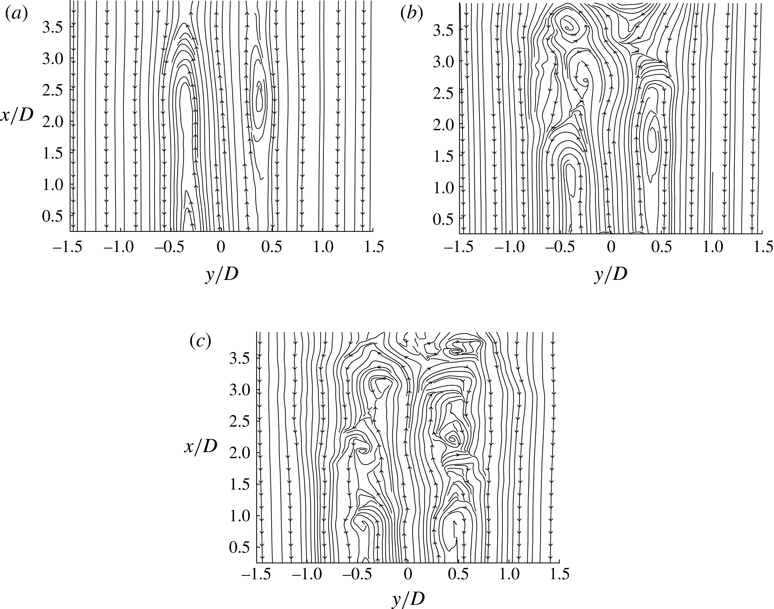
The flow showed distinctly different responses with Reynolds number, particularly for the three lowest helium cases. Figure 3 shows the instantaneous streamlines for these three flow conditions, where the axial velocity,
 $U$
, has been shifted by half of the jet exit velocity,
 $U_{j}$
. This shift is of the order of the convective velocity of the large-scale eddies in the shear layer. While these streamlines are two-dimensional representations of the three-dimensional flow, they help elucidate the local behaviour at different Reynolds numbers. These observations will be supported with additional metrics later. The images shown here were selected arbitrarily out of the 500 image pairs from each case, but they are representative of the typical flow. The exit location is just below the bottom of each flow field, as laser reflection off of the test fixture prevented accurate PIV measurements below
 $x/D\sim$
0.3.
Instantaneous streamlines for the velocity field of helium jets exhausting into air, shifted by
 $0.5U_{j}$
, for (a)
 $Re=1460$
, (b)
 $Re=2800$
, (c)
 $Re=5520$
.

At the lowest Reynolds number, shown in figure 3(a), the flow is organized and laminar within the field of view, with streamlines remaining parallel both inside and outside of the jet. On either side of the centreline, there is a shear layer centred approximately
 $0.35D$
away, which remains at this radial position throughout the test window. The shear layer does not appear to consist of distinct eddies, as the streamlines do not close until nearly the top of the test region. There are slight ripples to the streamlines on the exterior of the layer. However, outside of this minor disturbance, the flow remains laminar.
The flow shows a distinct change at the next Reynolds number, seen in figure 3(b). For the first two diameters downstream of the exit, the flow again appears laminar, with a clearly defined, organized shear layer. At
 $x/D\sim 2$
, the flow changes significantly, with a large-scale vortex seen forming on the left side of the image. The same response occurs on the right side of the image, slightly downstream at
 $x/D\sim 2.75$
. From these locations onward, the shear layer features larger disturbances than any observed in figure 3(a). This suggests that the flow is transitioning from a laminar to a turbulent condition. The asymmetric transition is seen in other image pairs, although the location is not constant. In some cases, the transition occurs on the right side first.
In figure 3(c), the streamlines are more typical of a turbulent jet, with perturbations over the entire axial range. In the imaged plane, counter-rotating vortices are observed at similar axial locations, indicative of axisymmetric vortex rings. These rings are spaced approximately one exit diameter apart, although their spacing becomes more variable with downstream distance. In the region considered, the disturbances do not reach the centreline, but there are deviations in the core flow. Similar flow responses are seen at the other two, higher Reynolds number cases.
It is critical to note that the transition process seen in figure 3 should not be confused with the pipe flow transition. Certainly, the three Reynolds numbers do correspond with the three regimes for pipe flow – laminar for
 $Re<2300$
, turbulent for
 $Re>4000$
, and transitional in between. However, this will just correspond to the exit flow conditions, not necessarily the behaviour downstream. Virtually all jets will transition to turbulence at some point, since small perturbations will grow for
 $Re>4$
(Drazin & Reid Reference Drazin and Reid1981). The transition point may occur at different locations depending on flow conditions (Dimotakis Reference Dimotakis2000). In this experiment, the transition is in the near-exit region at the intermediate Reynolds number.
5.2 Ensemble-averaged mean flow
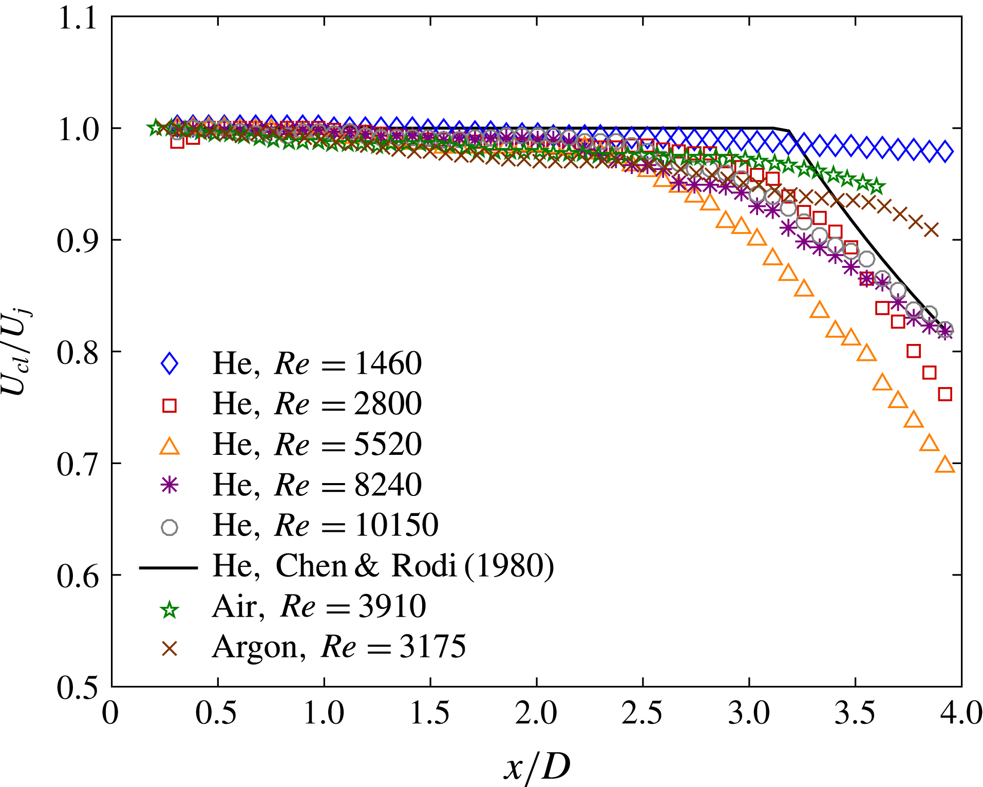
The differing instantaneous flow structures lead to clear differences in the ensemble-averaged flow response. Figure 4 displays the centreline velocity variation for the air, argon and helium cases considered. Here, the centreline velocity,
 $U_{cl}$
, is normalized by the exit velocity,
 $U_{j}$
. These profiles are determined by ensemble averaging all 500 processed vector fields, which were acquired over approximately four minutes at steady-state conditions. Also shown is the expected centreline curve for a turbulent helium jet, based on the study by Chen & Rodi (Reference Chen and Rodi1980). In the potential core,
 $U_{cl}/U_{j}\approx 1$
, while it falls off as
 $U_{cl}/U_{j}\approx 9.1D(\unicode[STIX]{x1D70C}_{j}/\unicode[STIX]{x1D70C}_{a})^{1/2}/(x-x_{u})$
farther downstream (Amielh et al.
Reference Amielh, Djeridane, Anselmet and Fulachier1996). Here,
 $x_{u}$
is a virtual origin, which depends on the gas. With helium, the virtual origin is at approximately
 $-0.2D$
, and the potential core length is approximately
 $3.2D$
. The centreline decay curves are not shown for air or argon, as the potential core extends beyond the test region.
Axial variation of ensemble-averaged centreline velocity with various gases and Reynolds numbers. Velocities are normalized by the exit velocity,
 $U_{j}$
. A quasi-analytical decay curve for turbulent helium jets is also shown. The overall velocity uncertainty in the jet is
 $\pm$
2.0 % of the centreline speed.

For all five helium cases, the centreline velocity is essentially unchanged over the first two diameters downstream of the exit. At the lowest
 $Re$
, where the jet flow remained laminar in figure 3(a), the velocity remains constant throughout the entire test region. This is similar to the behaviour seen at low
 $Re$
by Suresh et al. (Reference Suresh, Srinivasan, Sundararajan and Das2008). At the higher Reynolds numbers, the centreline velocity begins to drop at
 $x/D\sim 2$
, with most cases dropping to approximately 80 % of the exit velocity at
 $x/D\sim 4$
. These curves agree with the quasi-analytical curve from Chen & Rodi (Reference Chen and Rodi1980). There is some deviation for the moderate
 $Re$
cases, however. At
 $Re=2800$
, the initial decrease is more gradual, but the slope becomes more negative after
 $x/D\sim 3$
. This may be indicative of the sudden transition seen in figure 3(b). At
 $Re=5520$
, the centreline velocity falls further to approximately 70 % of the exit velocity, suggesting that the mixing is more rapid than at higher
 $Re$
. This is reminiscent of the entrainment increase seen by Ricou & Spalding (Reference Ricou and Spalding1961) at lower turbulent Reynolds numbers. The air and argon velocities show only a modest decrease over the test region, as they remain in their potential core.
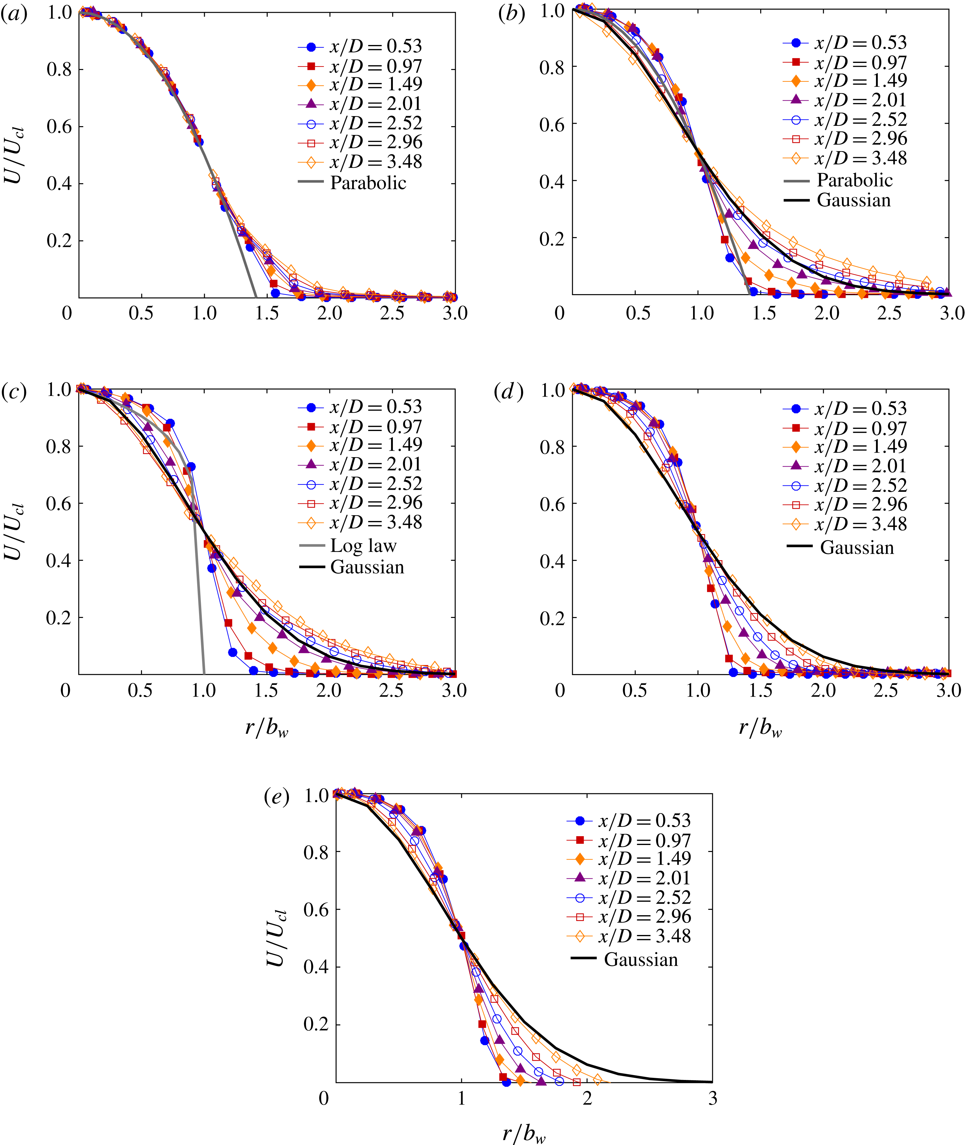
Figure 5 shows the ensemble-averaged velocity profiles for the three lowest
 $Re$
helium cases, air and argon at various downstream locations. The mean axial velocity,
 $U$
, is normalized by the centreline velocity, while the radial position,
 $r$
, is normalized by the jet half-width,
 $b_{w}$
. Here, the half-width is defined as the radial distance where the velocity falls to one half of the centreline speed.
Ensemble-averaged velocity profiles at various downstream locations for (a) helium 1, (b) helium 2, (c) helium 3, (d) air, (e) argon. For comparison, parabolic, log law and Gaussian profiles are also included. Velocities are normalized by the local centreline velocity,
 $U_{cl}$
. The lines connecting the data points are included to better distinguish the individual data sets, not to indicate additional measurements. Again the velocity uncertainty in the jet is
 $\pm$
2.0 % of the centreline speed.

In figure 5(a), the velocity profiles collapse over most of the radial positions, with no deviation outside of the uncertainty until approximately
 $1.2b_{w}$
. The profiles also overlap a parabolic profile, which would be expected for fully developed laminar pipe flow at the exit. This overlap corroborates the fact that flow is nearly fully developed for this lower Reynolds number. With such a profile,
 $U/U_{cl}=1-(2r/D)^{2}$
, the radius would correspond to
 $b_{w}\times 2^{1/2}$
, which agrees very well with the measured data. Travelling downstream, the profile only changes at its boundary, with a gradual diffusion outward. The velocity profile at the farthest downstream position has non-negligible magnitudes out to nearly
 $2.5b_{w}$
, so the profile deviates from parabolic over the outer
 $1.3b_{w}$
. Interestingly, this is comparable to the expected diffusion for a laminar boundary layer (White Reference White1991), even for this jet geometry. In laminar flow, the diffusion length should have a square root dependence on the axial distance traversed,
 $\unicode[STIX]{x0394}x$
. The viscous diffusion length scale is
 $L_{diff}=(\unicode[STIX]{x1D708}_{j}\unicode[STIX]{x0394}x/U_{j})^{1/2}$
, where
 $\unicode[STIX]{x1D708}_{j}$
is the jet kinematic viscosity. Over the three-diameter long axial range considered here,
 $L_{diff}$
is
 $0.11D$
. The laminar boundary-layer thickness is five times this scale, which is 0.55D or
 $1.6b_{w}$
, comparable to the
 $1.3b_{w}$
measured here. This is further evidence that the flow remains laminar throughout this entire test region.
Figure 5(b) shows the helium response at the intermediate Reynolds number. Up to
 $x/D\sim 2$
, the velocity profile in the core again agrees with a parabolic profile. The diffusion outside the jet is more rapid, however, with the profile already extending beyond
 $2.5b_{w}$
at this location. After this position, the velocity profile begins to spread in the core as well, with the speeds approaching the expected Gaussian shape for fully developed turbulent jets. The profile does differ significantly from Gaussian outside the jet, with speeds approximately 10 % higher out beyond
 $2.5b_{w}$
. Hence, we see that flow is initially comparable to the parabolic, laminar pipe flow profile, and then it rapidly transitions towards a more Gaussian turbulent profile. However, it is clearly still developing.
The third helium case, seen in figure 5(c), displays a faster diffusion process, as would be expected in a more turbulent flow. Nearest the exit, at
 $x/D=0.53$
, the profile is slightly fuller than a log law profile, which would be seen with turbulent fully developed pipe flow (White Reference White1991). While both cases have fairly uniform speeds up to
 $r\sim 0.8b_{w}$
, the measured jet profile has values approximately 5 % higher. At all axial positions, there is diffusion observed within the core and outside the jet, as the turbulent shear layer is developing. At the end of the test region, the mean velocity profile matches a Gaussian profile to within the uncertainty inside of one half-width, but the measured speeds are approximately 5 % higher outside of the jet core. Thus, the mean profile is close to fully developed within 4 diameters of the exit. This is comparable to levels observed in turbulent air jets (Mi et al.
Reference Mi, Kalt, Nathan and Wong2007) and helium jets (Amielh et al.
Reference Amielh, Djeridane, Anselmet and Fulachier1996). Of course, this does not mean the flow is fully developed, as the turbulence statistics may still be developing.
Although not displayed here, the jet half-width remains approximately constant over this axial range for all three helium Reynolds numbers. For the lowest
 $Re$
, the half-width is approximately
 $0.36D$
, which is almost exactly the value seen for a parabolic profile. At the intermediate
 $Re$
, the half-width is nearly the same value, and it varies by less than 10 % over this axial range. At the highest
 $Re$
, the half-width is approximately
 $0.45D$
, or closer to the actual radius at the exit.
The air and argon cases show similar profiles to one another, as seen in figure 5(d,e), respectively. The velocity responses of air and argon are approaching the Gaussian profile at the furthest downstream locations. Both profiles show less variation of the velocity as a function of downstream location when compared with the helium 2 and helium 3 cases.
Of the mean flow variables, the entrainment ratio is the most pertinent to analyses of plume density and stability. This parameter can be calculated in several ways, including analysis of half-width growth (Fischer et al. Reference Fischer, List, Koh, Imberger and Brooks1979), direct integration of the velocity profile (Amielh et al. Reference Amielh, Djeridane, Anselmet and Fulachier1996) and radial inflow analysis (Falcone & Cataldo Reference Falcone and Cataldo2003). Half-width growth may be misleading in the near-exit region, as this parameter does not vary much due to initial development. Velocity profile integration is limited by the radial extent of measurements, truncating the larger radii flows. Hence, the radial inflow is measured directly here, focusing on the entrained region outside of the jet. Since the entrained velocities were well below those in the jet core, they were analysed using the second PIV data set acquired with longer time delays.
This method is based on a differential control volume analysis, considering a cylindrical slice centred on the jet axis. The differential change in jet mass flow rate is due to ambient entrainment from the lateral sides of the cylinder
 $$\begin{eqnarray}\frac{\text{d}{\dot{m}}}{\text{d}x}=2\unicode[STIX]{x03C0}\unicode[STIX]{x1D70C}_{a}rv_{r}.\end{eqnarray}$$
Here,
 $v_{r}$
is the radially inward velocity at the position
 $r$
. At large radial distances, the quantity
 $rv_{r}$
is a constant. Typically, it is presented using an entrainment velocity,
 $w$
, which is referenced to the half-width position
 $$\begin{eqnarray}w=\frac{\lim _{r\rightarrow \infty }(rv_{r})}{b_{w}}.\end{eqnarray}$$
Note that this is not the actual velocity at this location, as the flow is usually radially outward there (Agrawal & Prasad Reference Agrawal and Prasad2003). The radial velocity measurements are used to calculate this limit, including data well outside the jet core, usually at least two half-widths from the centreline. Finally, this entrainment velocity is normalized by the centreline velocity, resulting in the entrainment ratio,
 $$\begin{eqnarray}\unicode[STIX]{x1D6FC}=\frac{w}{U_{cl}}.\end{eqnarray}$$
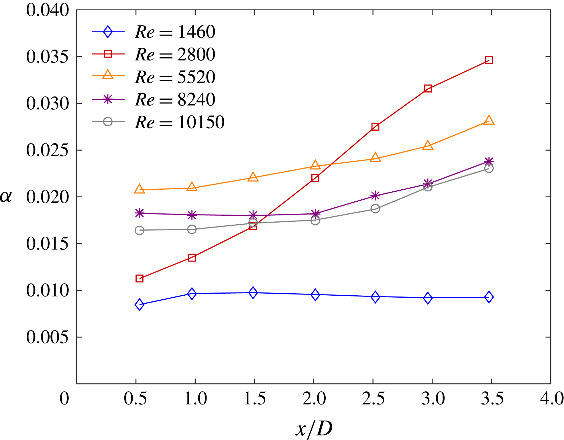
Figure 6 shows the entrainment ratio at various axial locations for the five Reynolds number cases with the helium jets. The magnitudes measured here agree with estimates based on direct integration of the velocity profile.
Axial variation of entrainment ratio with Reynolds number for the helium jets. The uncertainty in entrainment ratio is estimated at
 $\pm$
4.4 %.

At the lowest Reynolds number, the entrainment ratio is low, remaining relatively constant at 0.01 over the entire test range. This response is not surprising, as the low rate of diffusion would have smaller entrainment of ambient fluid. Also, since there is no significant change in the flow in this axial region,
 $\unicode[STIX]{x1D6FC}$
should be fairly constant.
For the highest three Reynolds numbers, the entrainment ratio is higher, as the turbulent eddies advect ambient fluid into the jet. The magnitudes here are closer to 0.02, with a gradual increase going downstream, as is usually seen in the developing region (Amielh et al.
Reference Amielh, Djeridane, Anselmet and Fulachier1996; Falcone & Cataldo Reference Falcone and Cataldo2003). For the lowest of these Reynolds numbers,
 $Re=5520$
, the entrainment ratio is approximately 20 % higher. This further corroborates the Reynolds number dependence seen by Ricou & Spalding (Reference Ricou and Spalding1961). It also agrees with the plane jet study from Namer & Ötügen (Reference Namer and Ötügen1988), which showed reduced mixing at higher
 $Re$
.
Most interesting, the intermediate Reynolds number shows a strong axial dependence in this range. At
 $Re=2800$
, the initial entrainment ratio is near 0.01, and then it rapidly rises to almost 0.035 by 3.5 diameters downstream of the exit. This lower value is consistent with the level at
 $Re=1460$
, before the flow transition, while the higher values are 50 % higher than the magnitudes for the more turbulent flows. However, if the total entrained mass flow is integrated across the entire axial range, the total would be comparable to those turbulent cases. Here, the entrainment ratio first surpasses the more turbulent level approximately two diameters from the exit, coinciding with the observed flow transition in figure 3(b). Measurements with the higher-density air and argon jets showed the same qualitative response at comparable
 $Re$
, although their uncertainty was considerably higher due to the reduced jet and entrained velocities.
When comparing to air jets, the entrainment ratio with helium is lower than the fully developed level of 0.06 (Falcone & Cataldo Reference Falcone and Cataldo2003). However, to correct for the density ratio, a square root dependence should be included, resulting in
 $\unicode[STIX]{x1D6FC}=\unicode[STIX]{x1D6FC}_{air}(\unicode[STIX]{x1D70C}_{j}/\unicode[STIX]{x1D70C}_{\unicode[STIX]{x1D6FC}})^{1/2}$
(Ricou & Spalding Reference Ricou and Spalding1961). This indicates that helium jets should have a value near 0.022 when fully developed. Thus, most values in figure 6 are in agreement with the measured data, particularly for the higher Reynolds number cases where
 $\unicode[STIX]{x1D6FC}$
has reached 0.022 by
 $x/D=3.5$
. Importantly, air jets typically reach their fully developed entrainment ratio more than 10 diameters downstream of the exit (Falcone & Cataldo Reference Falcone and Cataldo2003). With helium, however, the fully developed levels are already seen within the first three diameters from the exit, suggesting it is developing more rapidly. Since the test region is well inside the jet length, it is not practical to extrapolate to find the entrainment ratio for fully developed buoyant plumes.
5.3 Ensemble-averaged turbulence statistics
The velocity fluctuations are used to quantitatively examine the finer details of the flow response. By ensemble averaging the instantaneous fluctuations, the Reynolds stresses are evaluated. Specifically, this analysis includes the Reynolds normal stresses in the axial and radial directions, as well as the Reynolds shear stress.
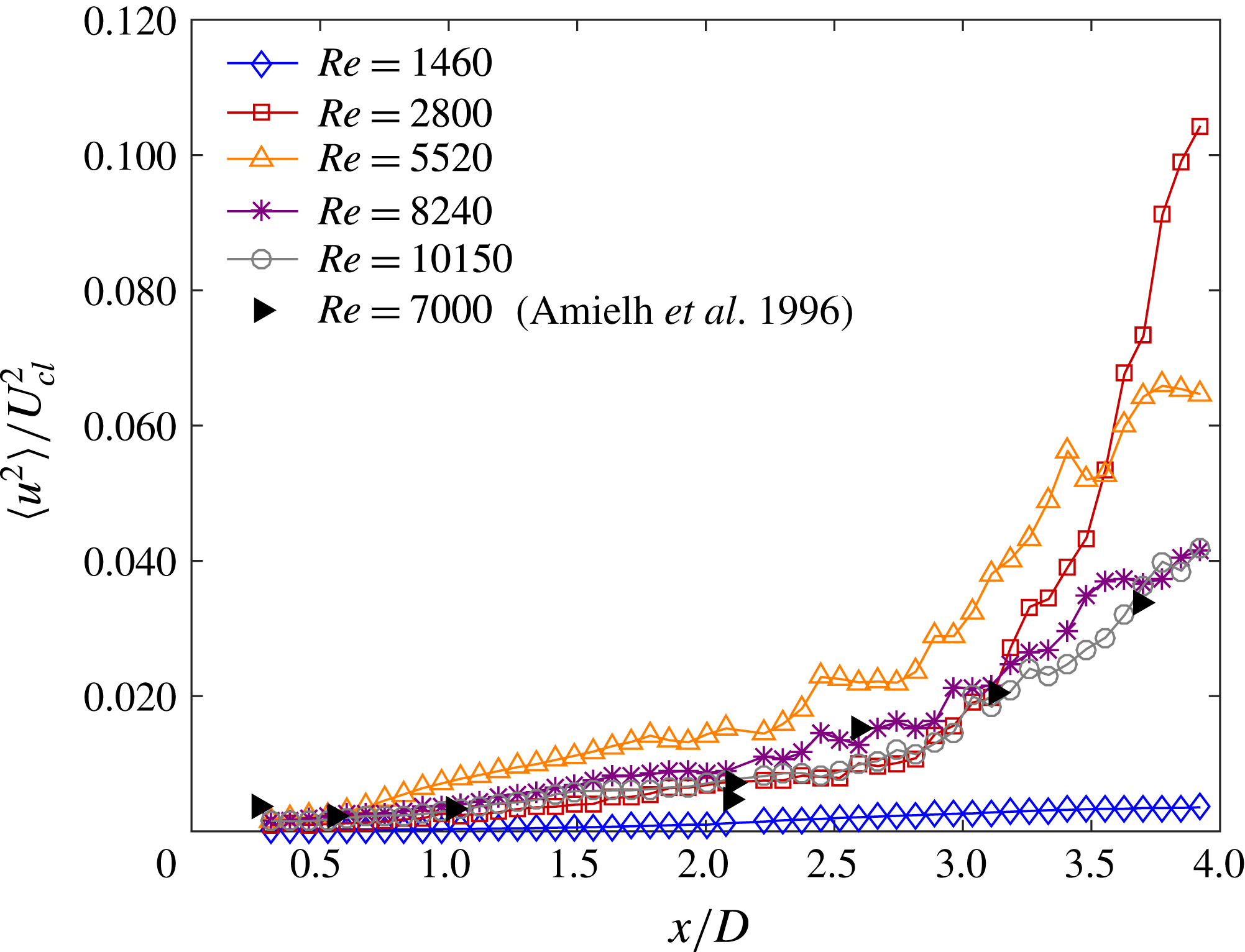
Figure 7 displays the Reynolds normal stress in the axial direction,
 $\langle u^{2}\rangle$
, along the centreline at various Reynolds numbers for helium. Here, the fluctuations are normalized by the local centreline velocity squared. Also shown are the LDV data from Amielh et al. (Reference Amielh, Djeridane, Anselmet and Fulachier1996), acquired at a comparable turbulent Reynolds number of 7000. The focus of this stress analysis is the dependence of Reynolds number; therefore, for clarity, air and argon are not included. Since the experiments are within the jet-like region, the buoyant effects are relatively small compared to the Reynolds number effects.
Axial variation of ensemble-averaged axial Reynolds normal stress with Reynolds number for the helium jets along the centreline. For comparison, the results from Amielh et al. (Reference Amielh, Djeridane, Anselmet and Fulachier1996) are included. Stresses are normalized by the local centreline velocity squared,
 $U_{cl}^{2}$
. The uncertainty of the turbulent fluctuation velocity is estimated at
 $\pm$
8.0 % of the peak axial fluctuations.

For all five cases shown, the normal stress grows in this developing region, although the magnitudes are almost negligible for the nearly laminar case, similar to the measurements by Suresh et al. (Reference Suresh, Srinivasan, Sundararajan and Das2008). The growth is gradual for the first three diameters, and then there is a more rapid rise, particularly at
 $Re=2800$
. In this intermediate, transitioning case, the turbulent stress rises by an order of magnitude between
 $x/D\sim 2.5$
and 4. The peak magnitude exceeds the fully developed level measured by Amielh et al. (Reference Amielh, Djeridane, Anselmet and Fulachier1996), which is below 0.09. This overshoot was also seen by Kyle & Sreenivasan (Reference Kyle and Sreenivasan1993) at
 $Re\sim 3000$
, where they observed a similar flow transition.
At higher Reynolds numbers, the measured normal stresses rise more gradually, with the results at
 $Re=8240$
and 10150 agreeing well with the measurements of Amielh et al. (Reference Amielh, Djeridane, Anselmet and Fulachier1996). For the more moderate Reynolds number of 5520, however, the magnitudes remain more than 50 % higher. These turbulence measurements are reasonable based on the entrainment ratio dependence seen in figure 6, as higher velocity fluctuations lead to more entrainment. Further, the large increase in normal stress at
 $Re=2800$
coincides with the rapid rise in entrainment.
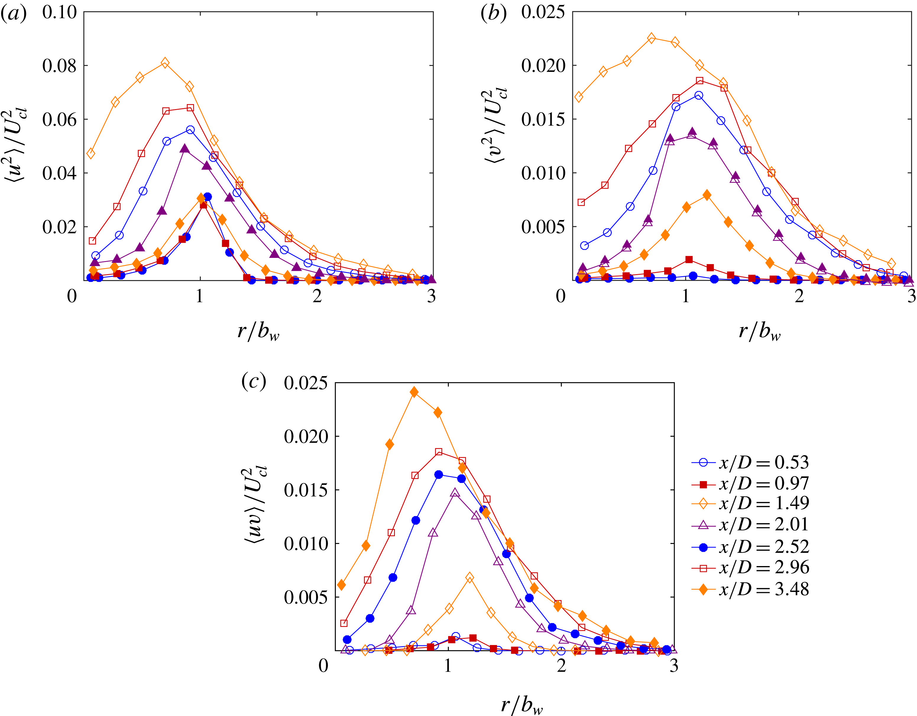
Ensemble-averaged profiles of helium 2 at various downstream locations for (a) axial Reynolds normal stress, (b) radial Reynolds normal stress and (c) Reynolds shear stress. Stresses are normalized by the local centreline velocity squared,
 $U_{cl}^{2}$
. For the Reynolds shear stress, the curves pass through zero at the centreline when considering PIV interrogation regions on both sides of the jet. The turbulent fluctuation velocity uncertainty is
 $\pm$
8.0 % of the peak axial fluctuations.

Figure 8(a–c) shows the axial development of the Reynolds stresses of helium at
 $Re=2800$
, displaying the axial normal,
 $\langle u^{2}\rangle$
, radial normal,
 $\langle v^{2}\rangle$
and shear stresses,
 $\langle uv\rangle$
, respectively. The profiles are normalized by the local centreline velocity squared, while the radii are normalized by the local half-width.
For all three stresses, the magnitudes are very low for the first 1.5 diameters downstream of the exit. Essentially, there is a single peak right at the half-width location, which defines the boundary of the jet. The radial normal and shear stresses start to increase by
 $x/D=1.5$
, but even these magnitudes are still very small. Afterward, the profiles show increased turbulent fluctuations across most radial locations, with the peak levels rising and diffusing both inward and outward. The peak continues to increase throughout the rest of the test region, and it moves inward to about
 $0.7b_{w}$
by 3.5 diameters downstream. Along the centreline, there is very little change in the normal stresses until approximately
 $x/D\sim 3$
, with a significant increase after this point. These profiles also begin to flatten out inside of one half-width. Overall, the flow is clearly developing throughout the entire test region, with the profiles continuing to evolve.
Still, the magnitudes of the turbulent statistics are already fairly high by
 $x/D\sim 3.5$
, at least when compared with other jet flows. For air jets in the fully developed region, Hussein, Capp & George (Reference Hussein, Capp and George1994) find peak magnitudes of
 $\langle u^{2}\rangle /U_{cl}^{2}\sim 0.08$
,
 $\langle v^{2}\rangle /U_{cl}^{2}\sim 0.045$
and
 $\langle uv\rangle /U_{cl}^{2}\sim 0.025$
. Amielh et al. (Reference Amielh, Djeridane, Anselmet and Fulachier1996) showed similar levels with helium jets. Here, peak values are found to be
 $\langle u^{2}\rangle /U_{cl}^{2}\sim 0.08$
,
 $\langle v^{2}\rangle /U_{cl}^{2}\sim 0.022$
and
 $\langle uv\rangle /U_{cl}^{2}\sim 0.024$
at
 $x/D$
of only 3.5. With the exception of the radial normal stress, the fluctuations are already approaching fully developed levels very near the exit. Thus, while the jets are developing throughout the test region, the evolution likely nears completion for
 $x/D$
just beyond 3.5. Hence, the measured entrainment levels should be close to the fully developed case, as observed in figure 6.
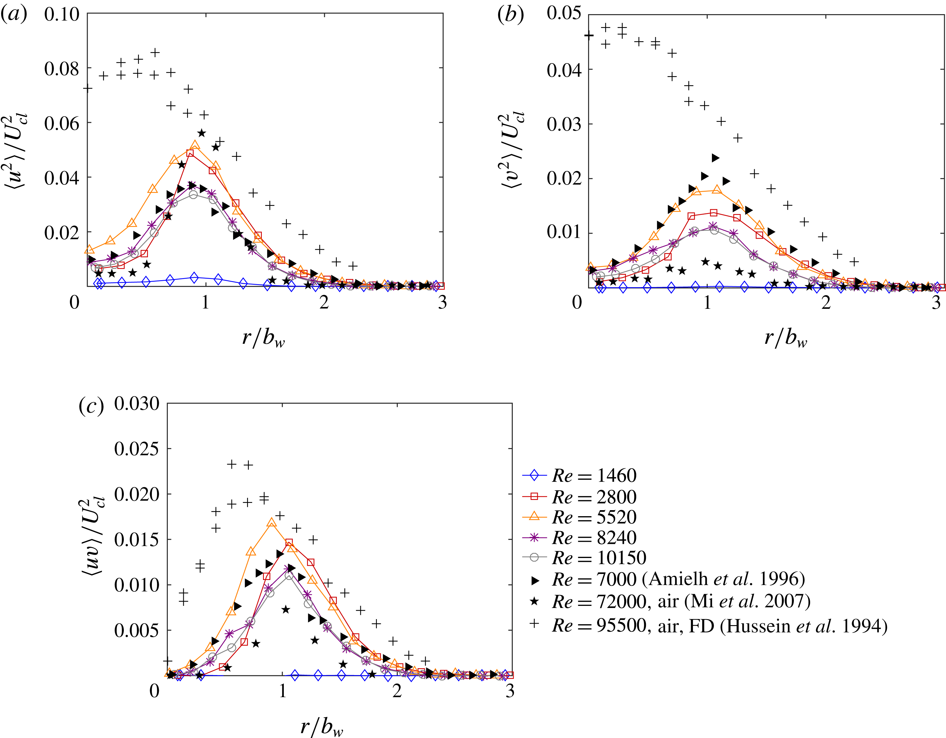
Figure 9(a–c) provides a broader comparison of the turbulent stress variation, showing the radial profiles of
 $\langle u^{2}\rangle$
,
 $\langle v^{2}\rangle$
and
 $\langle uv\rangle$
, respectively, for helium jets at different Reynolds numbers. Here, only profiles at
 $x/D\sim 2$
are shown, coinciding approximately with the transition location at
 $Re=2800$
. In addition, these figures include archival profiles from the developing region and the fully developed profile. The developing profiles were both acquired at the same location,
 $x/D=2$
, considering helium at
 $Re=7000$
(Amielh et al.
Reference Amielh, Djeridane, Anselmet and Fulachier1996) and air at a much higher
 $Re=72\,000$
(Mi et al.
Reference Mi, Kalt, Nathan and Wong2007). The fully developed profile was measured at
 $x/D=70$
with air at
 $Re=95\,500$
(Hussein et al.
Reference Hussein, Capp and George1994), although the data agree well with fully developed helium data (Panchapakesan & Lumley Reference Panchapakesan and Lumley1993).
Ensemble-averaged profiles for
 $x/D=2$
at various Reynolds numbers with helium jets for (a) axial Reynolds normal stress, (b) radial Reynolds normal stress and (c) Reynolds shear stress. Stresses are normalized by the local centreline velocity squared,
 $U_{cl}^{2}$
. The uncertainty of the turbulent fluctuation velocity is
 $\pm$
8.0 % of the peak axial fluctuations.

Similar to the axial variation seen in figure 7, the radial profiles show significant Reynolds number dependence at lower
 $Re$
. There are negligible fluctuations at the lowest Reynolds number of 1460, consistent with the observed laminar flow. For all other cases, there is a peak located near one half-width, with magnitudes diffusing away in either direction. The highest magnitudes are seen at
 $Re$
= 2800 and 5520, nearest to the transition, while the profiles nearly collapse at higher Reynolds number.
Examining the earlier studies, there is excellent agreement with Amielh et al. (Reference Amielh, Djeridane, Anselmet and Fulachier1996) at higher
 $Re$
for both
 $\langle u^{2}\rangle$
and
 $\langle uv\rangle$
. At
 $Re=8240$
and 10 150, the radial normal stress,
 $\langle v^{2}\rangle$
, is somewhat lower than seen in that previous study. However, there is agreement within the uncertainty at
 $Re=5520$
. Thus, the behaviour is comparable to that earlier helium study, in spite of differences in nozzle and ambient flow conditions. Compared to air (Mi et al.
Reference Mi, Kalt, Nathan and Wong2007), the axial normal stress is similar, but the radial normal and shear stresses are significantly higher here. This is consistent with a more rapid development with the lower-density gas. Finally, magnitudes at
 $x/D\sim 2$
are much lower than seen with a fully developed jet (Hussein et al.
Reference Hussein, Capp and George1994). However, as observed in figure 8(a,c) for
 $Re=2800$
, the peak levels at
 $x/D\sim 3.5$
nearly reach the fully developed magnitudes.
The velocity and Reynolds shear stress profiles may be used to estimate the entrainment ratio, as described in detail by Kaminski et al. (Reference Kaminski, Tait and Carazzo2005). Although their method requires information on the radial density profile, we can make an approximation by assuming a top-hat profile for the jet density. Using this technique, we find very low
 $\unicode[STIX]{x1D6FC}$
at
 $Re=1460$
,
 $\unicode[STIX]{x1D6FC}\sim 0.025$
at moderate
 $Re$
and
 $\unicode[STIX]{x1D6FC}\sim 0.02$
at higher
 $Re$
. These magnitudes agree well with the data in figure 6, even with the top-hat assumption.
Considering these turbulence statistics in full, the lower-density helium jet develops more rapidly than an air jet. There is even faster development at lower Reynolds number, with a peak at
 $Re=2800$
that exceeds fully developed levels. This may be partly an artefact of the averaging process, since the exact transition location varies slightly over time. Hence, for
 $x/D$
near this point, the flow will be intermittently laminar and turbulent, leading to larger fluctuations. However, because these higher levels persist for a couple of diameters beyond
 $x/D\sim 2$
, it is probable that the increased fluctuations are also due to the turbulent flow structures.
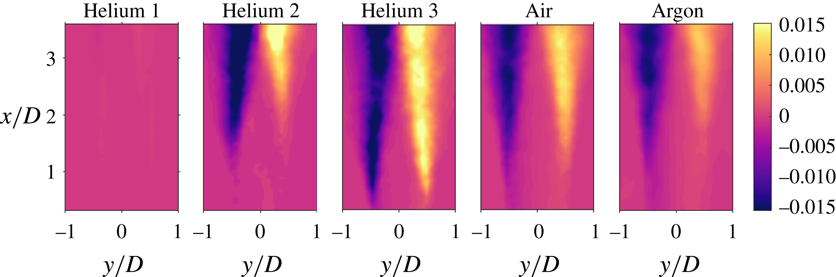
To examine the density variation, the Reynolds shear stress,
 $\langle uv\rangle$
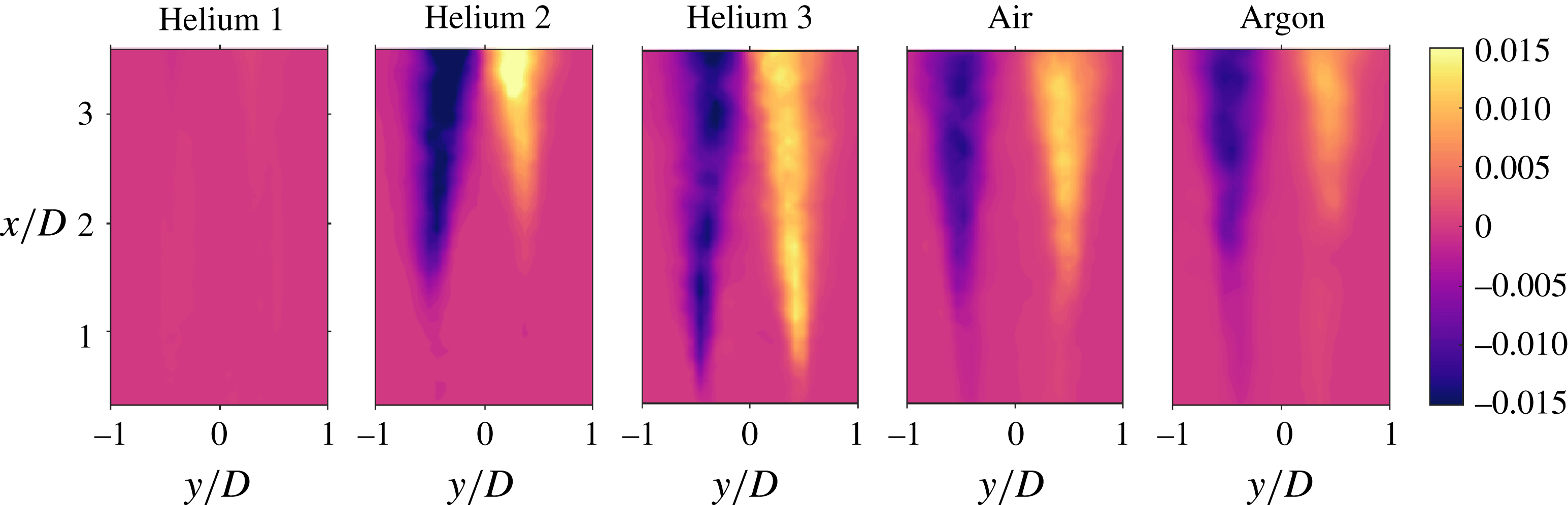
, is depicted in figure 10 for the first three cases of helium, air and argon. The value of
 $\langle uv\rangle$
is normalized by the square of the local centreline velocity,
 $U_{cl}^{2}$
, and the spatial locations are normalized by the exit diameter of the jet. For consistency with application of the analysis techniques used herein, the radial position of the jet will be referred to as
 $y$
for the remainder of the paper. In the experimental field of view, the jet progresses from the laminar to turbulent regime within the first three cases of helium. For clarity, the two highest
 $Re$
cases are not shown. Helium 1 has insignificant Reynolds shear stresses within the downstream locations in the experimental field of view. As the Reynolds number increases to 2800, helium 2, the shear stresses are present at
 $x/D\sim 1.5$
. Near the exit of the jet, shear stresses are negligible. Helium 2 also has a consistent level of high stresses across the mixing layers. This is the only case that shows uniform intensity when stresses are present. The most turbulent case of helium has high shear stresses that develop near the exit at
 $x/D=0.5$
, as seen in the helium 3 case in figure 10. For both helium 2 and helium 3, the Reynolds shear stresses develop quickly at
 $x/D\sim 1.5$
and
 $x/D=0.5$
, respectively. More specifically, the gradient within the jet is large for each case. As the Reynolds number increases from 1460 to 2800 the normalized Reynolds shear stress average value increases by over 5000 % while the change in the average shear stress for the
 $Re$
increase from 2800 to 5520 is 63 %, emphasizing the importance of
 $Re$
on Reynolds shear stress. The dependence of the Reynolds shear stress on
 $Re$
, especially in the low turbulence regime, is also observed qualitatively in figure 10.
For air as the medium exiting the jet, the shear stresses start to develop near the exit of the jet. The developed stresses are along the outside of the jet with a larger diameter of negligible shear stress in the centre. The shear stresses associated with argon exhibit a similar trend. The stresses again develop along the outer edge of the jet but occur farther downstream at
 $x/D\sim 1.5$
. The difference in downstream development of stresses for air and argon could be due to the Reynolds numbers associated with the two cases.
The two cases with the lowest Richardson numbers, air and argon, have a small gradient with respect to downstream direction when compared with the two cases of helium that contain shear stresses, helium 2 and helium 3. The average Reynolds stress values for air and argon, when compared with helium 2, increase by 4 % and decrease by 12 %, respectively, which could be attributed to slower development of the jet. The ensemble-averaged statistical analysis results can be used as reference for comparison with the reconstructed flow fields obtained by proper orthogonal decomposition.
The Reynolds shear stress,
 $\langle uv\rangle$
, with respect to
 $x$
and
 $y$
locations. Velocities are normalized by the local centreline velocity squared,
 $U_{cl}^{2}$
, and spatial locations are normalized by the exit diameter,
 $D$
.

5.4 Quadrant analysis
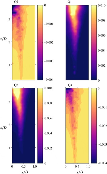
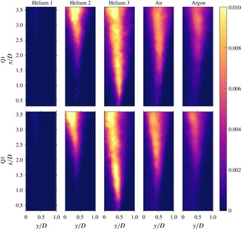
Quadrant analysis with respect to Reynolds shear stress is performed with results shown in figures 11 and 12. Figure 11 shows all four quadrants for the helium 2 case. The Reynolds shear stress for both figures is again normalized by the square of local centreline velocity, and the spatial locations are normalized with respect to the exit diameter of the jet. The analysis, as applied to the right side of the jet, shows Reynolds shear stresses dominating in the impeding-flow entrainment and advancing-flow ejection regions, with negligible contributions from the remaining two quadrants. Sreenivasan & Antonia (Reference Sreenivasan and Antonia1978) also observed that Q1 and Q3 had large contributions when compared with Q2 and Q4. In figure 11, the shear stresses develop at
 $x/D\sim 2$
for both of the dominant quadrants for helium 2. The development of the shear stresses confirms the initiation of turbulence at the corresponding downstream location.
Quadrant analysis with respect to Reynolds shear stress of helium 2 for half of the jet, specifically
 $0\leqslant y/D\leqslant 1$
.

Quadrant analysis with respect to Reynolds shear stress for the first and third quadrant for
 $0\leqslant y/D\leqslant 1$
.

Figure 12 shows Q1 and Q3 for the three low
 $Re$
cases of helium, air and argon, the other two quadrants follow the same trend as seen in figure 11 and are therefore excluded from further discussion. Again, helium 4 and 5 are excluded for clarity. Helium 1 shows negligible shear stresses in the dominant quadrants, reinforcing the conclusion that turbulence is not present in the provided field of view. As the
 $Re$
number increases to 2800 with helium as the medium, turbulence starts to develop around
 $x/D=2$
, where Reynolds shear stresses become prominent. Therefore, transition from nearly laminar to turbulent is observed as the jet develops downstream. It is also evident that at
 $x/D>3$
impeding-flow entrainment, Q3, occurs closer to the core of the jet while advancing-flow ejections, Q1, develop along the outside of the jet. With
 $Re$
of 5520, helium 3 appears to be fully turbulent with Reynolds shear stresses developing quickly, at a downstream location of
 $x/D=0.5$
. Similar to helium 2, stresses develop along the outside and closer to the core of the jet for Q1 and Q3, respectively for helium 3. The development and magnitude of the stresses present in Q3 correlate to the entrainment ratio profiles of helium 1, 2 and 3 depicted in figure 6.
The small gradient with respect to downstream direction for the air and argon cases, depicted in figure 10, also appears in figure 12. The shear stresses start to appear near
 $x/D=0.5$
for the jet of air but the development is gradual with an average of Q1 and Q3 containing 31 % less stress when compared to the average of the two quadrants of helium 3. Argon has similar characteristics as air, developing a jet of weak stresses quickly at
 $x/D=1.5$
, with a steady increase in stress with increasing downstream location. The delayed development of stresses in the downstream location for argon when compared to air is clearly depicted, similar to the trends seen in figure 10. Argon has an average of 42 % less stress intensity than helium 3. Air and argon continue to follow the trend of impeding-flow entrainment occurring closer to the core and advancing-flow ejections present along the outer edge of the jet, but both regimes are shifted away from the centre of the jet. More specifically, at
 $x/D=3.5$
for helium 3, shear stresses in quadrant 3 occur from
 $0\leqslant y/D\leqslant 0.4$
, whereas for air at 3.5
 $D$
downstream, significant stresses appear in the range of approximately
 $0.2\leqslant y/D\leqslant 0.6$
.
It is of note that the frequency occupation of quadrant 3 is greater than quadrant 1, with the location of these stresses present along the outside of the jet. This indicates that impeding-flow entrainment occurs more frequently than advancing-flow ejections for all cases considered. The high frequency locations do not agree with the locations of the high intensity stresses associated with Q3. This conveys that minute velocity fluctuations are occurring with great frequency along the outside of the mixing layer, but the large entrainment contributors are present along the inside of the mixing layer, as indicated in figure 12.
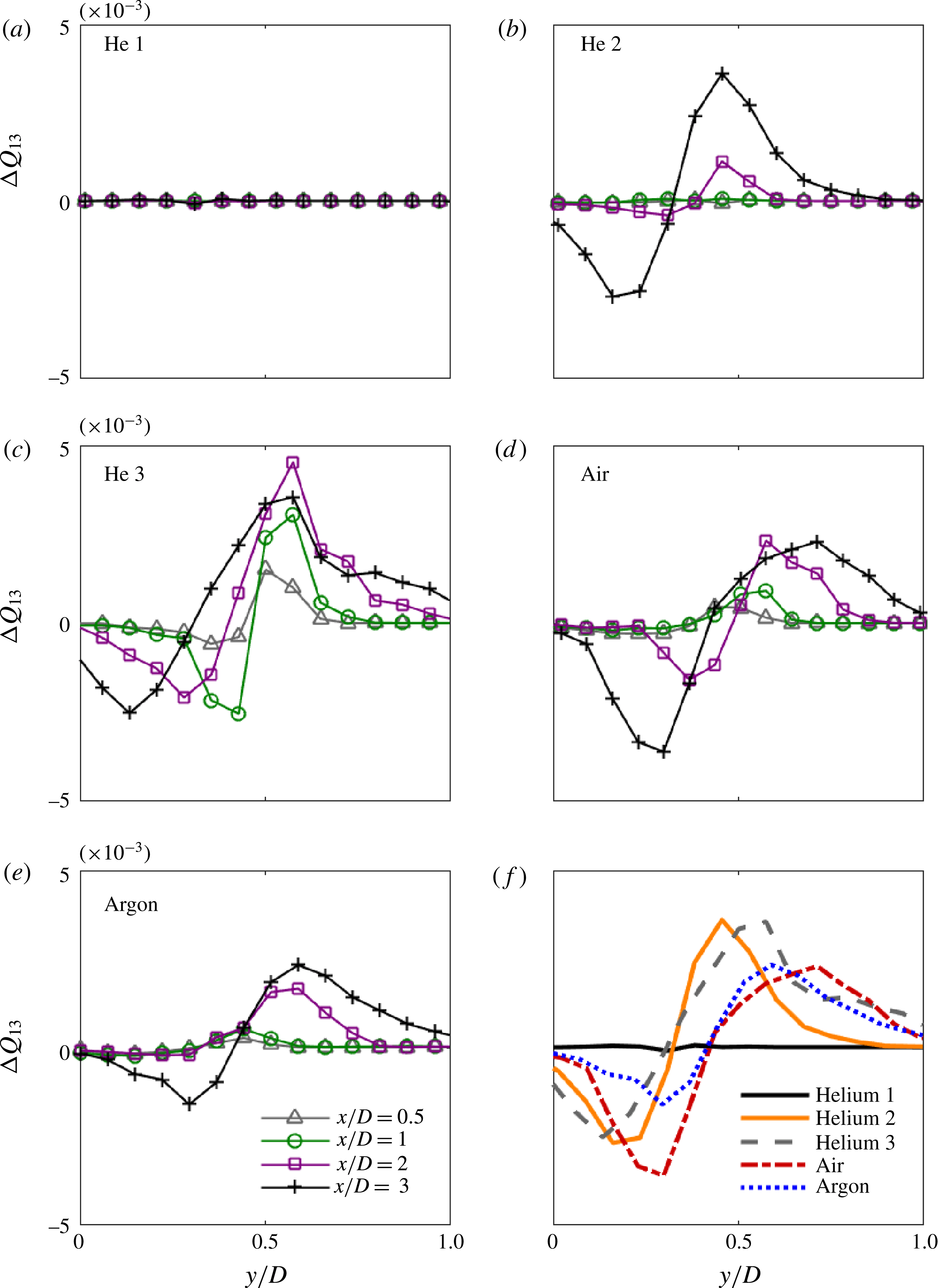
Profiles of the normalized Reynolds shear stress for the difference of Q1 and Q3,
 $\unicode[STIX]{x0394}Q_{13}$
, with respect to normalized spanwise location are shown in figures 13(a)–13(e). For each case shown, four respective streamwise locations,
 $x/D=0.5$
,
 $x/D=1$
,
 $x/D=2$
and
 $x/D=3$
, are plotted to show changes in shear stress corresponding to downstream location of the developing jet. Figure 13(f) shows the profile of
 $\unicode[STIX]{x0394}Q_{13}$
as a function of spanwise location at 3
 $D$
downstream for the considered cases. Figure 13(f) is included for comparison of downstream stress characteristics among the different cases. For all cases shown, excluding helium 1,
 $\unicode[STIX]{x0394}Q_{13}$
is negative from the centre of the jet until
 $y/D=0.25{-}0.5$
. The inflection point shifts from case to case and according to downstream location, with the higher downstream locations having inflection points earlier. For example, the profile of helium 3 at
 $x/D=3$
has an inflection point around
 $y/D=0.25$
, while at
 $x/D=0.5$
the profile shows an inflection point around
 $y/D=0.4$
. Past the inflection point,
 $\unicode[STIX]{x0394}Q_{13}$
shifts to positive values. This equates to Q3 (impeding-flow ejections) contributing more toward the centre of the jet and larger contributions toward the edge of the jet for Q1 (advancing-flow ejections).
Profiles of
 $\unicode[STIX]{x0394}Q_{13}$
with respect to spanwise location at four downstream locations;
 $x/D=0.5$
,
 $x/D=1$
,
 $x/D=2$
and
 $x/D=3$
for all cases. Profiles of
 $\unicode[STIX]{x0394}Q_{13}$
at 3
 $D$
downstream for each case are shown in (f).

The helium 1 case shown in figure 13(a) displays negligible Reynolds shear stresses in the jet, consistent with previous plots in indicating the jet contains laminar characteristics in the test field of view. The second case of helium agrees with previous observations that the jet contains transitional characteristics due to the absence of stresses until the downstream location of
 $x/D=2$
. Figure 13 also shows the consistent intensity of high level stresses present across the mixing layer at
 $x/D=3$
, as seen in figure 10. The third case of helium shows similar profiles for all downstream locations. The slight increase from
 $x/D=0.5$
to
 $x/D=1$
indicates that the flow is fully developed turbulent flow prior to the downstream location of
 $x/D=1$
. Figure 13(f) verifies the development of helium 2 at the downstream location of
 $x/D=3$
when compared with helium 3, due to the similarity of the curves.
Air and argon, figure 13(d,e), have a similar shape and smoothness of the curves for
 $\unicode[STIX]{x0394}Q_{13}$
. Both plots also show that the shear stresses increase with increasing downstream location. The extended tails and smoothness of the plots of air and argon indicate that the jets have a wider distribution of flow in the spanwise direction. The smoothness of the profiles of air and argon is emphasized in figure 13(f) when compared with the sharp curves of the more turbulent helium cases. The developing mixing layer present along the outside of the jet for air and argon is consistent with these observations taken from figure 10 and can be attributed to Richardson number.
5.5 Swirling strength and correlation coefficients
The instantaneous streamlines shown in figure 3 clearly show the presence of eddies, at least within the centre of the shear layer. These streamlines are calculated in a reference frame shifted by 50 % of the jet speed, resulting in a relative axial velocity,
 $U_{rel}$
, of (
 $U-0.5U_{j}$
). This reference is selected because it is the convective velocity at the half-width location. Eddies moving near this speed will be displayed, but others moving at different speeds may not be apparent. Vorticity can also be used to identify eddies, as it is reference-frame independent. However, vorticity can be significant in strong shear layers with no turbulent eddies, such as seen in figure 3(a). Therefore, another reference-independent metric is used to identify the eddies in the instantaneous fields.
Here, the swirling strength is determined, using the eigenvalues of the local velocity gradient tensor to identify regions with swirling motion (Adrian, Christensen & Liu Reference Adrian, Christensen and Liu2000). At each location in the two-dimensional flow field, a velocity gradient tensor is formed:
 $$\begin{eqnarray}\unicode[STIX]{x1D63F}_{2-D}=\left(\begin{array}{@{}cc@{}}\displaystyle \frac{\unicode[STIX]{x2202}u}{\unicode[STIX]{x2202}x} & \displaystyle \frac{\unicode[STIX]{x2202}u}{\unicode[STIX]{x2202}y}\\ \displaystyle \frac{\unicode[STIX]{x2202}v}{\unicode[STIX]{x2202}x} & \displaystyle \frac{\unicode[STIX]{x2202}v}{\unicode[STIX]{x2202}y}\end{array}\right).\end{eqnarray}$$
Here,
 $u$
and
 $v$
represent the streamwise and spanwise instantaneous velocity, respectively. The eigenvalues of this tensor are either both real valued or else complex conjugates, with the latter case being more common:
 $$\begin{eqnarray}\unicode[STIX]{x1D740}=\unicode[STIX]{x1D706}_{cr}\pm \text{i}\unicode[STIX]{x1D706}_{ci}.\end{eqnarray}$$
The inverse of the complex part,
 $1/\unicode[STIX]{x1D706}_{ci}$
, is related to the period of the swirling motion. For pure shear flow, the swirling strength
 $\unicode[STIX]{x1D706}_{ci}$
is zero, while concentrated eddies have a finite magnitude. Thus, regions with a non-zero swirling strength can be identified as eddies.
Figure 14 shows the swirling strength contours for the same three instantaneous vector fields seen in figure 3. Here, the complex part of the eigenvalue is normalized by the exit speed,
 $U_{j}$
, and diameter,
 $D$
. For all three images, the contour levels are the same.
Instantaneous swirling strength contours for helium jets at (a)
 $Re=1460$
, (b)
 $Re=2800$
, (c)
 $Re=5520$
. Contours are normalized by the exit speed and diameter as
 $\unicode[STIX]{x1D706}_{ci}D/U_{j}$
.

For the almost laminar case, seen in figure 14(a), the swirling strength contours have small magnitudes throughout the imaged region. Most of these are weak disturbances, whose magnitude is comparable to the uncertainty in the velocity measurements. There are two diffuse structures in the shear layer that extend over a broad region, centred approximately at
 $x/D\sim 2.5$
, but even these magnitudes are relatively small when compared to higher Reynolds numbers. These locations do coincide with the closed streamlines seen in figure 3(a). However, it appears that there are no significant eddies present in this case, as expected by the low entrainment and turbulence statistics.
In the transitioning flow, shown in figure 14(b), several peaks are present in the swirling strength contours. Most of these eddies coincide with vortical motion in the instantaneous streamlines of figure 3(b). The first strong disturbances are seen near the transition point close to
 $x/D\sim 2$
. There are at least two pairs of vortices located on either side of the centreline, at approximately
 $x/D\sim 2.5$
and 3.5, but there are also single eddies at
 $x/D\sim 1.42$
and 3.77. This indicates that the eddies are not wholly axisymmetric, with clear three-dimensional variation. Further, the strongest peak is seen near the centreline at
 $x/D\sim 3.41$
, and there is no additional vortex of similar strength at this location. Hence, this flow condition clearly has strong, non-axisymmetric eddies.
For the turbulent flow condition, displayed in figure 14(c), the large-scale pattern is more structured. Pairs of similar-strength vortices are seen on either side of the centreline at
 $x/D\sim 1$
, 2 and 3, indicative of vortex rings. There is some distortion in the arrangement of the ring at
 $x/D\sim 3$
, but the flow is mostly axisymmetric. In addition to these larger eddies, there are numerous smaller-scale disturbances, clearly showing the turbulent nature of the flow. Eddies are also seen near the exit, unlike at lower Reynolds numbers. However, the flow does not have the distinct three-dimensional variation seen at
 $Re=2800$
.
Two-point spatial correlations provide another method of examining the eddy structure. Here, the relationship between velocity fluctuations is investigated at a basis point (
 $y_{o}$
,
 $x_{o}$
) relative to another location (
 $y_{o}+\unicode[STIX]{x1D6FF}y,x_{o}+\unicode[STIX]{x1D6FF}x$
). For an instantaneous vector field, the velocity fluctuations,
 $v$
, at these locations are multiplied together. The average multiple is determined over all measured fields, and it is normalized by the average fluctuations at the basis point, resulting in the spatial correlation coefficient
 $$\begin{eqnarray}R_{vv}=\frac{\langle v(y_{o},x_{o})v(y_{o}+\unicode[STIX]{x1D6FF}y,x_{o}+\unicode[STIX]{x1D6FF}x)\rangle }{\langle v(y_{o},x_{o})\rangle \langle v(y_{o},x_{o})\rangle }.\end{eqnarray}$$
Correlations can be determined for axial (
 $uu$
), radial (
 $vv$
), and cross (
 $uv$
) fluctuations. Only radial correlations will be shown here, as they provide sufficient information about the eddy behaviour.
Figure 15 displays the spatial correlation contours for the radial fluctuations of the helium jet at the intermediate Reynolds number
 $Re=2800$
. Basis points are considered at three axial positions,
 $x/D=1$
, 2 and 3, located approximately in the middle of the shear layer on the left side of the image, with
 $y/D=-0.5$
. This is equivalent to a radial location of
 $r/D=0.5$
. In these images, the contours range from
 $-1$
to 1. A value of 1 indicates perfect correlation, while a value of
 $-1$
indicates perfect anti-correlation.
Radial spatial correlation coefficient contours for
 $Re=2800$
relative to a basis point at
 $y/D=-0.5$
and (a)
 $x/D=1$
, (b)
 $x/D=2$
, (c)
 $x/D=3$
.

At the location nearest the exit,
 $x/D=1$
, there are clear relationships between fluctuations at this position and locations farther downstream. As seen in figure 15(a), there is a strong anti-correlation with a region centred at
 $x/D=1.78$
, followed by a strong correlation with a region centred at
 $x/D=2.67$
. These strong interactions are seen in spite of the low magnitude of the fluctuations upstream of the flow transition, shown in figure 7. In fact, this leads to spatial correlation coefficients exceeding 1 in magnitude, since the velocity fluctuations are so much larger downstream of the transition. This result is an artefact of the definition of the correlation given in (5.6), not an unphysical response. Interestingly, there are also correlations and anti-correlations seen on the opposite side of the centreline. Overall, these contours suggest that the flow experiences axisymmetric, oscillating disturbances upstream of the transition, reminiscent of the Kelvin–Helmholtz instability. These disturbances also have an influence beyond the transition point.
Closer to the transition location, at
 $x/D=2$
, there is a strong peak with a significant spatial extent. Figure 15(b) shows that the correlation coefficient exceeds 0.2 over a near-circular region with a diameter of
 $0.60D$
. In addition, there are significant anti-correlations with locations centred at
 $x/D=1.34$
and 2.67, with
 $R_{vv}$
near
 $-0.35$
at each position. This indicates that radial inflow at
 $x/D=2$
coincides with radial outflow at positions approximately
 $0.67D$
away axially, suggesting an eddy size of the same order of magnitude. Unlike at
 $x/D=1$
, there is little correlation with positions on the opposite side of the centreline, suggesting that the structures are no longer axisymmetric.
At the most downstream location considered,
 $x/D=3$
, there is still a strong peak with similar spatial extent. Here, the correlation coefficient contours depicted in figure 15(c) exceed 0.2 over a region with a diameter of
 $0.62D$
, only slightly larger than at
 $x/D=2$
. There is still an anti-correlation with an upstream position, with
 $R_{vv}$
near
 $-0.31$
at
 $x/D=2.01$
. The image window is too small to accurately discern the correlation farther downstream. Still, this suggests that there are eddies slightly larger than
 $0.6D$
in diameter. As with the previous location, there is no significant correlation across the centreline, so the eddy structures are unlikely to be axisymmetric.
Figure 16 shows the radial spatial correlation contours of helium at the higher, more turbulent Reynolds number of 5520. The same three basis point locations are considered for comparison, and the contour levels again range from
 $-1$
to 1.
Radial spatial correlation coefficient contours for
 $Re=5520$
relative to
 $y/D=-0.5$
and (a)
 $x/D=1$
, (b)
 $x/D=2$
, (c)
 $x/D=3$
.

Nearest the exit, shown in figure 16(a), there is a small region of correlation around the peak at
 $x/D=1$
. The contours exceed 0.2 over an approximately circular region with a diameter of
 $0.40D$
. There is an anti-correlation with fluctuations at
 $x/D=1.49$
, and both these peaks are mirrored on the opposite side of the centreline. This organized response suggests the presence of a vortex ring, whose extent is of the order of
 $0.5D$
. Unlike at
 $Re=2800$
, there is no clear relationship with structures farther downstream.
At
 $x/D=2$
, seen in figure 16(b), the correlated peak increases in size. The contours exceed 0.2 over a slightly elliptical region with a diameter of
 $0.52D$
, with the extent slightly larger in the radial direction. There is no significant anti-correlation at this position, with almost no locations having
 $R_{vv}$
below
 $-0.2$
. The vortex ring structure seen near
 $x/D=1$
is now absent. Compared with the transitioning case in figure 15(b), the spatial extent of the correlation here is smaller, even though the velocity fluctuations seen in figure 7 are larger.
For the most downstream position in figure 16(c), the spatial correlation continues to increase in size. Now, the peak is clearly elliptical, with the contours above 0.2 over
 $0.76D$
radially and
 $0.54D$
axially. In the radial direction, the correlation nearly reaches the centreline. There is still negligible anti-correlation, and the response across the centreline is independent of these fluctuations. At this location, the spatial extent of the eddies is now comparable to that of the intermediate Reynolds number, as seen in figure 15(c).
Examining the suite of spatial correlation coefficients, the eddy growth is distinctly different between the helium cases at
 $Re=2800$
and 5520. For the lower, transitioning case, larger-scale eddies begin to form immediately after flow transition near
 $x/D=2$
, with spatial extent of the order of
 $0.67D$
. The eddies also have significant anti-correlation with locations almost one diameter away, further emphasizing their large size. In the higher, more turbulent case, eddies are seen closer to the exit. Their size is initially smaller, approximately
 $0.4D$
in diameter, as would be expected in the thinner shear layer. Farther downstream, these eddies grow larger and more elliptical, reaching to approximately
 $0.65D$
by
 $x/D=3$
. However, there is much less anti-correlation at this higher Reynolds number, indicating the spatial extent is more limited in this developing region.
5.6 Proper orthogonal decomposition
Figure 17 shows two representations of the distribution of energy for the three lowest
 $Re$
cases of helium, air and argon. Eigenfunctions represent the modes of turbulence and eigenvalues,
 $\unicode[STIX]{x1D740}$
, and measure the energy associated with each eigenfunction where the total turbulence kinetic energy equals the summation of the eigenvalues, as in (3.12). The energy content of the eigenvalues is shown in figure 17(a). The eigenvalues are self-normalized, where
 $K_{n}=\unicode[STIX]{x1D706}_{n}/\sum _{i=1}^{N}\unicode[STIX]{x1D706}_{i}$
, so energy contained in the
 $n$
th mode is normalized by the total energy. The first mode contains the most energy, with a substantial decrease in energy as modes increase. Cases of helium 1 and argon show the largest normalized contributions from the first mode and a sharp decrease as the mode number increases when compared with the other cases. The remaining three profiles show comparatively less energy in the first mode and exhibit a more gradual decline in successive modes. Figure 17(b) shows the percentage of successive contribution of the eigenvalues to the total turbulence kinetic energy. This allows for a clear comparison of the convergence rate of the different cases. The eigenvalues or energy contained in the first
 $n$
modes are normalized by the total energy and written as
 $$\begin{eqnarray}Z_{n}=\frac{\displaystyle \mathop{\sum }_{k=1}^{n}\unicode[STIX]{x1D706}_{k}}{\displaystyle \mathop{\sum }_{i=1}^{N}\unicode[STIX]{x1D706}_{i}},\quad n=1,2,\ldots ,N.\end{eqnarray}$$
Similar to figure 17(a), argon and helium 1 have a rapid convergence in comparison to the other three cases, which collapse on top of each other.
The distribution of energy described by (a) normalized eigenvalues,
 $K_{n}$
, and (b) successive summation of eigenvalues,
 $Z_{n}$
as a function of the mode,
 $n$
.

Table 2 details the corresponding modes for 50, 75 and 95 % reconstruction of kinetic energy to lower degrees of freedom. Table 2 also presents the turbulent kinetic energy,
 $E$
, from equation (3.12), multiplied by the density of the medium. Most of the energy, 95 %, is within 337 modes with at least 50 % of the energy within only 37 modes for all cases examined. There is an observed dependence of
 $Ri$
and
 $Re$
on the relative turbulent kinetic energy. It appears that as the Reynolds number increases, the energy increases. A similar trend is observed for the Richardson number. More specifically, while air, argon and helium 2 have similar Reynolds numbers, argon contains only two thirds of the relative turbulent kinetic energy of air and one tenth of the relative energy of helium 2.
Corresponding eigenmodes required for 50, 75 and 95 % reconstruction and turbulence kinetic energy for each case.
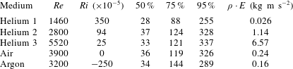
Figure 18 shows the POD modes 1–4, 10 and 250 for the five considered cases with respect to streamwise and spanwise location. The eigenmodes are self-normalized and the spatial locations are normalized by the jet diameter. The colour bar is omitted from the figure because the locations and patterns of the structures are of the quantities of interest. Mode 1, containing the most energetic structures, shows a large variance from case to case. For helium 1, the first mode is null, indicating low energy present in the jet within the field of view. Argon shows a similar trend with insignificant structures present in mode 1. Helium 2 has non-axisymmetric energetic structures present far downstream in the jet, suggesting the jet develops its largest contribution of energy close to
 $x/D=2.5$
. Helium 3 has axisymmetric structures present along the entire vertical length of the jet, illustrating the quick development of the shear stress. Air has slender structures that run along the outside of the jet, with the most energetic structures present far downstream.
The second mode for helium 2, helium 3 and air have similar structures to those present in their respective first mode. The second and third eigenmodes for helium 1 start to resemble Fourier modes, indicating homogeneous behaviour with respect to shear stress fluctuations. As the mode increases, modes 4 and 10 are once again null for helium 1, indicating an absence of energetic structures within the test field of view. Argon begins to resemble air as the modes increase, with long slender structures that span all downstream locations along the edges of the jet. Helium 2 starts to show structures closer to the exit of the jet for modes 3 and 4, demonstrating that the development of turbulence is occurring closer to
 $x/D=1.5$
, but that most of the energy associated with helium 2 is present farther downstream at
 $x/D=2.5$
. Helium 3 contains structures that progress from far downstream for modes 3 and 4 to near the exit of the jet for mode 10, verifying the presence of structures throughout the plume. Apart from helium 1, there exists similarity among the four cases for the tenth eigenmode, with structures existing along the outside of the jet. The characteristics of the modes of helium 3 agree with trends observed by both Caraballo et al. (Reference Caraballo, Samimy, Scott, Narayanan and Debonis2003) and Tinney, Glauser & Ukeiley (Reference Tinney, Glauser and Ukeiley2008) on high speed turbulent jet data. Tinney et al. (Reference Tinney, Glauser and Ukeiley2008) investigated an axisymmetric converging nozzle and observed that lower-order modes dominate the potential core while high index modes dominate the low-speed side of the mixing layer. Caraballo et al. (Reference Caraballo, Samimy, Scott, Narayanan and Debonis2003) found that in the near-jet region the first two modes contained axisymmetric structures and that successive, less energetic modes, contained asymmetric structures.
Mode 250 highlights the development of the jet again. Helium 1 shows small structures that are independent of downstream location. Helium 2 contains structures along the outside of the jet until around
 $2.5D$
downstream. Helium 3 shows a similar trend but the width of the jet is greater and the structures start to conjoin in the centre at approximately
 $1D$
downstream. The presence of small structures in the centre of the jet for helium 2 and 3 indicates that the jet is developing turbulent behaviour at those locations. Air and argon show similar characteristics for mode 250. The width of the jet grows with increasing downstream location but the core remains non-turbulent.
POD modes 1–4, 10 and 250 corresponding to all five cases as indicated in the figure.

The effects of buoyancy and non-buoyancy driven flow are best seen by comparing helium 2 and argon. Helium 2 contains energetic structures while argon, which has a similar Reynolds number, does not. This indicates that the lower-density gas exhibits turbulent structures earlier in the developing jet. For the second and third cases of helium, structures containing large amounts of turbulence kinetic energy occur closer to the centre of the jet. In contrast, air and argon contain energetic structures toward the edges of the jet. Although this shift between cases is observed throughout all modes presented in figure 18, it is more pronounced in the first and second eigenmodes. Features present along the edge of the jet indicate high Reynolds shear stress in the mixing layer due to the interface with the ambient air (Tennekes & Lumley Reference Tennekes and Lumley1972). The presence of energetic structures along the edge of the jet versus the centre is observed to correlate with the magnitude of the Richardson number. Helium as the medium is less dense than the ambient fluid, resulting in a buoyant jet when compared with argon and air. This produces energetic structures closer to the core. Argon is more dense than air resulting in eigenmodes that show an absence of energetic structures toward the centre of the jet.
Figure 19 shows the deployment of 50 % reconstruction for Reynolds shear stress. In comparison with figure 10, the magnitude of the shear stress has diminished slightly with reconstruction, but the location and intensity of stresses are consistent for each case. Helium 3 is still the largest contributor to Reynolds shear stress with the case of helium 1 having, once again, insignificant stresses present.
POD 50 % reconstruction of Reynolds shear stress,
 $\langle uv\rangle$
, for all cases normalized by local centre line velocity,
 $U_{cl}^{2}$
.

6 Discussion
The phenomena examined here illuminate several intriguing features of the turbulence near a transitioning, variable-density jet with geophysical applications for
 $Re$
below
 $10^{4}$
and
 $Ri$
with magnitudes near 0.001 (i.e. fumaroles, springs and gas vents). The most distinct aspect occurs for helium at the intermediate Reynolds number of 2800, where the entrainment and turbulence statistics increase significantly about the transition point. These variables even exceed the magnitudes seen for fully turbulent jets at the same axial location, as seen in figure 9(a–c). The turbulent fluctuations for helium are also slightly larger at a low turbulent Reynolds number of 5520, before reaching a consistent response for
 $Re>8000$
. This demonstrates that there is a Reynolds number dependence for the turbulence in this regime.
The turbulence fluctuations are larger near transition for at least three reasons. First, there may be large deviations due to transient variation in the local transition point, with intermittent laminar and turbulent conditions at nearby axial locations. Second, the flow exhibits clear three-dimensionality, with strong, non-axisymmetric eddies observed immediately after transition, as shown in figure 14. This is comparable to the instabilities observed by Monkewitz et al. (Reference Monkewitz, Lehmann, Barsikow and Bechert1989) for heated air jets. Third, the eddies are large after transition, displaying a spatial influence of more than 0.6 diameters, as seen in figure 15. For more turbulent Reynolds numbers, the eddies grow with the shear layer, depicted in figure 16. These structures do not attain a similar scale until downstream of the transition point. In short, the sudden, three-dimensional transition leads to larger eddies and greater local mixing.
Beyond these Reynolds number effects, significant differences were observed for the low-density jet compared to a non-buoyant jet. In particular, the flow develops more quickly than a non-buoyant jet, approaching a fully developed velocity profile within only four diameters of the exit, as seen in figure 5(c). The turbulent statistics also grow more rapidly with the lower density, depicted in figure 9(a–c). As noted by Gharbi et al. (Reference Gharbi, Amielh and Anselmet1995), lighter gases typically experience more rapid mixing. However, this should not be construed as a buoyancy effect in this near-exit region, since the flow is still dominated by the exit jet inertia. Still, the low inertia of the helium jet should permit more rapid entrainment by higher-density air, just as observed here.
Returning to the original problem of plume entrainment, these measurements illustrate several significant issues. First, the assumption of a constant entrainment ratio is not valid for low Reynolds numbers, particularly close to the transition point. The eddies are larger and non-axisymmetric in this vicinity, producing greater turbulent fluctuations and corresponding entrainment. Even beyond the transition, there is more fluctuation and entrainment at lower turbulent Reynolds numbers.
For natural flows, this result suggests a sort of sweet spot in entrainment rate with the size of the feature. Very small fumaroles, springs and gas vents whose flow regime is transitional are likely to produce better mixing than smaller, laminar ones or larger, fully turbulent flows. Specifically, fumaroles would become buoyant more rapidly in this Reynolds number regime, reducing the hazards observed when they collapse. Similarly, particles near sublacustrine springs would disperse more significantly in this regime. In engineering applications where efficient mixing is crucial, this regime and its improved mixing might be designed into the flow.
Because of the rapid flow development of low-density jets, as observed in the helium experiments presented here, it may be reasonable to assume a constant entrainment ratio soon after the exit. This differs from neutrally buoyant or negatively buoyant gases like
 $\text{CO}_{2}$
, which may take more than 20 diameters to achieve fully developed conditions (Falcone & Cataldo Reference Falcone and Cataldo2003). For these heavier gases, this results in reduced air entrainment (Solovitz et al.
Reference Solovitz, Mastin and Saffaraval2011), potentially shifting the criterion for achieving buoyancy and increasing local density. However, care must be applied in assuming fully developed flow at low density, as many flows may also be overpressured. Under those conditions, even helium jets have longer development lengths (Saffaraval et al.
Reference Saffaraval, Solovitz, Ogden and Mastin2012).
Quadrant analysis of the cases shows that impeding-flow entrainment and advancing-flow ejections dominate for free shear flow. The large contribution to shear stress from these two quadrants indicates that fluctuations are driven by entrainment along the inside of the mixing layer and the streamwise mean flow along the outside of the mixing layer. Impeding-flow entrainment, acting against the mean streamwise flow, illustrates that the majority of mixing in the near-vent region of the jet is occurring on the inside of the mixing layer. This observation is validated by the relationship between the intensity of shear stresses in the dominant quadrants and the Richardson number. Between cases it also appears that the Richardson number is correlated to the location of the stresses in the spanwise direction while the Reynolds number is correlated to the development of shear stresses in the streamwise direction. This observation is further validated by the difference of the two quadrants, Q1 and Q3. From figure 13(a–e),
 $\unicode[STIX]{x0394}Q_{13}$
indicates that as the Reynolds number increases, shear stresses are present closer to the exit of the jet. The difference in the quadrants also shows the smaller gradient and bias toward the outer edge of the jet that is present when Richardson number decreases.
 $\unicode[STIX]{x0394}Q_{13}$
provides insight into the mechanisms of the flow. From the analysis performed, it is clear that the mechanism for entrainment is quadrant 3, which impedes the flow while the mechanism along the outside of the jet is observed as quadrant 1, advancing-flow ejections. For understanding of alternative mechanisms of the fluctuating velocity components, further analysis must be performed.
Proper orthogonal decomposition yielded similar results. Figure 18 depicts a dependence of the energetic structure shape and location on the Reynolds and Richardson numbers. Turbulence develops more quickly as
 $Re$
increases, while shear stresses are present farther from the core of the jet as
 $Ri$
decreases. There is also an observed correlation between the relative turbulence kinetic energy and both the Reynolds and Richardson numbers from table 2. The turbulence kinetic energy increases with both an increasing
 $Re$
and an increasing
 $Ri$
. Reconstruction of the Reynolds shear stresses with 50 % of the total turbulence kinetic energy exhibits a minor reduction in the magnitude, but the shape and location of the stresses are consistent with the full-order model for all cases shown.
The reduced-order description, using at most 37 degrees of freedom, can be used for further analysis in place of the full-order model. The eigenmodes obtained from POD present a set of mathematical expressions and the low-order description allows for lower computational time for analysis on the variable-density jet. Classification of the events obtained from quadrant analysis leads to better understanding of entrainment and its dependence on parameters in geophysical flows. The resulting closure model, also obtained from quadrant analysis, completes a mathematical representation of the flow to allow for equations to be formed to better predict flow characteristics based on the flow structures of the data. More specifically, the low-order model obtained from POD and the closure model from quadrant analysis equations can provide a model to adjust for adequate resolution when setting up models by identifying what kind of structures occur and where they are most prominent.
7 Conclusions
The behaviour of variable-density jets is studied at conditions pertinent to some geophysical phenomena, specifically at Reynolds numbers below 10 000 and Richardson numbers with magnitudes of the order of 0.001. The flow was examined for a variety of conditions, ranging from a stable, nearly laminar jet to a fully turbulent jet. Examining these results, several distinct features were observed.
First, for a flow transitioning near the exit, there is a sharp increase in local entrainment and turbulent fluctuations. The magnitudes exceed the fully developed turbulent levels at some locations. This increase is due to the non-axisymmetric, three-dimensional nature of the eddies after transition. These eddies also extend over a larger region than observed for turbulent jets at the same axial location.
Second, at lower Reynolds numbers, turbulent jets have higher entrainment and velocity fluctuations than experienced at
 $Re>8000$
. The entrainment at
 $Re>8000$
is below the levels observed near transition, as the eddies are smaller in size. In addition, the turbulent eddies are initially axisymmetric, growing along with the shear layer.
Third, lower-density jets experience more rapid development than non-buoyant flows, both in the mean velocity and the turbulent fluctuations. However, the turbulent statistics are still far from fully developed by
 $x/D=4$
, the end of the range examined.
Finally, the Reynolds number is observed to influence the development of the stresses and where they occur in the downstream location. The effect of the Richardson number is not as easily quantifiable. Analysis of the five cases indicates that the location of the stresses in the spanwise direction is dependent on the Richardson number. There also appears to be a correlation between the gradient of the developing stresses in the spanwise direction and the Richardson number, but this connection is complicated by the effects of the Reynolds number. Further research, with a greater selection of Richardson numbers should be performed to validate the discussed observations.
Acknowledgements
This work is supported by a grant (NSF-EAR-1346580) from the U.S. National Science Foundation. The authors greatly appreciate the assistance of K. Roberts, C. Button and F. Deets in the laboratory. The authors also wish to thank C. Swanson and T. Dunmire for their technical contributions. All PIV vector fields used in this work are stored in the ENCS database at WSU Vancouver. Access may be attained by contacting the corresponding author.