1. Introduction
Most species of fish swim in schools during their daily lives, and their remarkable coordination and exceptional manoeuvrability in schools have attracted significant research interest across multiple disciplines, including physics, biology and bio-inspired robotics (Krebs Reference Krebs1976; Larsson Reference Larsson2012; Ko, Lauder & Nagpal Reference Ko, Lauder and Nagpal2023). A long-standing conjecture is that hydrodynamic interactions not only mediate the collective motion, but also confer hydrodynamic benefits to individuals in schools (Weihs Reference Weihs1973; Lighthill Reference Lighthill1975). However, this hypothesis has remained contentious, owing to the persistent inconsistencies between theoretical and experimental results (Partridge & Pitcher Reference Partridge and Pitcher1979; Ashraf et al. Reference Ashraf, Godoy-Diana, Halloy, Collignon and Thiria2016, Reference Ashraf, Bradshaw, Ha, Halloy, Godoy-Diana and Thiria2017; Filella et al. Reference Filella, Nadal, Sire, Kanso and Eloy2018). Consequently, the role of hydrodynamic interactions in fish schooling behaviour remains poorly understood (Ko et al. Reference Ko, Lauder and Nagpal2023). One of the primary challenges is that the hydrodynamic interactions between living fish are complex and hard to analyse (Yang & Zeng Reference Yang and Zeng2024).
To further investigate the hydrodynamic interactions in a fish school, the group can be simplified into a model consisting of two flapping foils or hydrofoils arranged in regular formations (Maertens, Gao & Triantafyllou Reference Maertens, Gao and Triantafyllou2017; Ambolkar & Arumuru Reference Ambolkar and Arumuru2022). Numerous experimental and numerical studies have demonstrated that individuals can achieve significant hydrodynamic benefits when positioned in a variety of well-organised formations, including the tandem, staggered and side-by-side formations (Dewey et al. Reference Dewey, Quinn, Boschitsch and Smits2014; Muscutt, Weymouth & Ganapathisubramani Reference Muscutt, Weymouth and Ganapathisubramani2017; Lagopoulos, Weymouth & Ganapathisubramani Reference Lagopoulos, Weymouth and Ganapathisubramani2020; Pan & Dong Reference Pan and Dong2022; Pourfarzan & Wong Reference Pourfarzan and Wong2022; Xu et al. Reference Xu, Xu, Li and Yang2023; Handy-Cardenas, Zhu & Breuer Reference Handy-Cardenas, Zhu and Breuer2025). In the tandem formation, the performance enhancement of the leader is primarily the result of the push effect generated by the follower, particularly when the gap is small (Maertens et al. Reference Maertens, Gao and Triantafyllou2017; Pourfarzan & Wong Reference Pourfarzan and Wong2022). Meanwhile, the performance augmentation of the follower is attributed to the increase of its effective angle of attack, especially when it weaves between vortices shed from its leader (Muscutt et al. Reference Muscutt, Weymouth and Ganapathisubramani2017; Xu et al. Reference Xu, Xu, Li and Yang2023). In the side-by-side formation, the performance of the bodies is determined by their lateral interference, which depends on the lateral gap and phase difference between them (Dewey et al. Reference Dewey, Quinn, Boschitsch and Smits2014). However, a key limitation of these previous studies is that the regular formations and the motion of each body are artificially prescribed. Thus the feedback of bodies to the surrounding flow is neglected. Consequently, the emergent stability and self-organisation capability of such regular formations remain poorly understood.
On the other hand, considering the wake–body coupling in the longitudinal direction, the fish school can be simplified as a model consisting of two tandem flapping foils or hydrofoils, which respectively can self-propel along the longitudinal direction (Zhu, He & Zhang Reference Zhu, He and Zhang2014a ; Yu, Lu & Huang Reference Yu, Lu and Huang2021). Several previous studies have demonstrated that swimmers can spontaneously form stable and regular formations in the longitudinal direction, only through the hydrodynamic interactions (Ramananarivo et al. Reference Ramananarivo, Fang, Oza, Zhang and Ristroph2016; Newbolt, Zhang & Ristroph Reference Newbolt, Zhang and Ristroph2019; Heydari & Kanso Reference Heydari and Kanso2021; Lin, Liu & Wu Reference Lin, Liu and Wu2024; Chae & Jeong Reference Chae and Jeong2025; Nitsche, Oza & Siegel Reference Nitsche, Oza and Siegel2025). Moreover, the longitudinal scales of these formations can be quantified as integers, with the phase difference and the motion wavelength of the leader (Lin et al. Reference Lin, Wu, Zhang and Yang2019). Furthermore, compared with an isolated swimmer, the downstream swimmer exhibits significant energy savings in these configurations, since it can exploit the vortex-induced lateral flow to reduce its oscillating drag (Zhu et al. Reference Zhu, He and Zhang2014a ; Lin et al. Reference Lin, Liu and Wu2024). Additionally, the speed enhancement can be achieved by the collective in several small-gap formations (Ramananarivo et al. Reference Ramananarivo, Fang, Oza, Zhang and Ristroph2016; Lin et al. Reference Lin, Wu, Zhang and Yang2019). On the other hand, several studies have demonstrated that the lateral flow interactions significantly influence the longitudinal self-organisation of collectives (Peng, Huang & Lu Reference Peng, Huang and Lu2018; Newbolt, Zhang & Ristroph Reference Newbolt, Zhang and Ristroph2022; Jeong, Kim & Lee Reference Jeong, Kim and Lee2023; Ormonde et al. Reference Ormonde, Kurt, Mivehchi and Moored2024). However, these self-propelled models employed in prior studies were only free to move longitudinally, with their lateral motion constrained. Therefore, this simplification neglects the lateral self-organisation of fish schools.
Recently, to further investigate the hydrodynamic interactions in fish schools, the system has been simplified as two flapping foils or hydrofoils with two degrees of freedom (longitudinal and lateral) (Gazzola et al. Reference Gazzola, Chatelain, van Rees and Koumoutsakos2011). Interestingly, the results have revealed that swimmers can achieve equilibrium distances in both lateral and longitudinal directions (Lin et al. Reference Lin, Wu, Zhang and Yang2021, Reference Lin, Wu, Yang and Dong2022). That is, swimmers can achieve two-dimensionally stable, regular formations only via the hydrodynamic interactions. Meanwhile, in most of such regular formations, the swimmers have hydrodynamic benefits, including speed enhancement and efficiency improvement (Lin et al. Reference Lin, Wu, Zhang and Yang2021, Reference Lin, Wu, Yang and Dong2022). However, the undulatory motion – a fundamental kinematic characteristic of fish swimming – was not considered in these aforementioned studies (Lin et al. Reference Lin, Wu, Zhang and Yang2021, Reference Lin, Wu, Yang and Dong2022). Moreover, only two specific scenarios (in-phase and anti-phase) were considered in these studies (Lin et al. Reference Lin, Wu, Zhang and Yang2021, Reference Lin, Wu, Yang and Dong2022). In reality, the experimental observations have revealed that fish can adjust their wavelength and phase difference within a large range according to the surrounding flow (Ashraf et al. Reference Ashraf, Godoy-Diana, Halloy, Collignon and Thiria2016, Reference Ashraf, Bradshaw, Ha, Halloy, Godoy-Diana and Thiria2017). However, few studies have focused on the coupling effects of wavelength and phase difference on the flow-mediated self-organisation of fish schools. Consequently, the effects of wavelength and phase difference on fish schooling behaviour remain poorly understood. This is the motivation of the current work.
Sketch view of the simulation model. Here,
 $G_x$
and
 $G_y$
respectively denote the longitudinal and lateral distances between the two fish,
 $u_x$
and
 $u_y$
respectively represent the longitudinal and lateral speeds of each fish, the subscripts 1 and 2 correspond to fish 1 and fish 2, respectively, and
 $\lambda$
is the wavelength of the travelling wave over the fish body.

To better understand the hydrodynamic interactions in fish schools, the coupling effects of the wavelength and phase difference on the collective motion of two undulatory swimmers, who can self-propel in both longitudinal and lateral directions, are numerically studied in this paper. As shown in figure 1, the fish school is simplified as two undulated swimmers initially arranged in the side-by-side formation. The aim of the present study is to demonstrate how the undulatory swimmers spontaneously form stable formations via the hydrodynamic interactions, and further to examine the modulating roles of phase difference and wavelength in such a flow-mediated self-organisation process. The remainder of this paper is organised as follows. The problem description and methodology are presented in § 2. The simulation results are addressed in detail with discussion in § 3. Finally, some conclusions are drawn in § 4.
2. Problem description and methodology
As shown in figure 1, the fish school is simplified as two parallel swimmers, which can self-propel in both longitudinal and lateral directions. The NACA 0012 aerofoil with chord length denoted as
 $c$
is used as the profile of each swimmer. The undulating motion of each fish is simplified as
 \begin{align} y_{1}(x,t) &= A(x)\cos(kx-2\pi\kern-0.5pt\textit{ft}), \end{align}
 \begin{align} y_{2}(x,t) &= A(x)\cos(kx-2\pi\kern-0.5pt\textit{ft} + \varphi ), \end{align}
 \begin{align} A(x) &= A_{0}-A_{1}x+A_{2}x^2,\quad 0\leqslant x \leqslant 1, \end{align}
where
 $y_{1}(x,t)$
and
 $y_{2}(x,t)$
denote the lateral displacements of fish 1 and fish 2, respectively,
 $x$
is the longitudinal coordinate along each fish,
 $k=2\pi /\lambda$
is the wavenumber,
 $\lambda$
is the wavelength of the travelling wave over the fish body, and
 $A(x)$
is the undulated amplitude along the fish body, which is determined by the coefficients
 $A_{0}(=0.02)$
,
 $A_{1}(=0.08)$
and
 $A_{2}(=0.16)$
.
In this paper, each fish can self-propel in both longitudinal and lateral directions, which is controlled by the Newton’s second law, i.e.
 \begin{equation} M\frac {\text{d}^2\boldsymbol{X}_{i}}{\text{d}t^2} = \boldsymbol{F}_i, \end{equation}
where
 $M$
is the mass of each fish, which is defined as
 $M=\rho _{s}S$
, for
 $\rho _{s}$
and
 $S$
respectively the density and area of each fish. In this paper, the mass of fish is controlled by the mass ratio
 $\bar{M}=M / M_f=1.0$
, where
 $M_f=\rho S$
is the mass of flow with the same area of fish,
 $\rho$
is the density of flow. Here,
 $\boldsymbol{X}_i=(X_i,Y_i)$
is the position of each fish, and
 $\boldsymbol{F}_i=(F_{ix},F_{iy})$
is the force applied on surface of each fish,
 $i=1,2$
representing fish 1 and fish 2, respectively. Thus the separation distance between two fish is defined as
 $G_x=X_1-X_2$
,
 $G_y=Y_1-Y_2$
.
Thus the swimming speed of each fish is defined as
 \begin{equation} u_{ix} = -{\text{d}X_{i}}/{\text{d}t},\quad u_{iy} = {\text{d}Y_{i}}/{\text{d}t}. \end{equation}
The cycle-averaged speed is calculated as
 \begin{equation} \bar{u}_{ix} = \frac {1}{T} \int _t^{t+T} {u_{ix}(t)} \,\text{d}t, \quad \bar{u}_{iy} = \frac {1}{T} \int _t^{t+T} {u_{iy}(t)} \,\text{d}t. \end{equation}
The power consumption is calculated as
 \begin{equation} P_{i}(t) = \oint _{s} F_{iy}{\kern-0.5pt}V_{iy}\,\text{d}s, \end{equation}
where
 $F_{iy}$
and
 $V_{iy}$
are respectively the instantaneous lateral force and lateral oscillating speed per unit length on the surface of each fish.
It should be pointed out that when a stable formation is achieved, the cycle-averaged lateral speed of each fish is close to zero, and the cycle-averaged longitudinal speeds are equal to each other, i.e.
 $\bar{u}_{iy} \approx 0$
,
 $\bar{u}_{1x} = \bar{u}_{2x} = \bar{u}_{x}$
. Thus the propulsive efficiency of each fish can be quantified by the cost of transport (
 $\textit{CoT}$
), which is defined as the power consumption per unit mass to swim a unit distance in the longitudinal direction (Wu et al. Reference Wu, Shu, Lee and Wan2022a
), i.e.
 \begin{equation} \textit{CoT}_{i} = \bar{P}_{i} / (M\bar{u}_{x}), \end{equation}
where
 $\bar{P} = {1}/{T} \int _t^{t+T} P(t) \,\text{d}t$
is the cycle-averaged power consumption. For the fish school,
 $\textit{CoT}$
is calculated as
 $\textit{CoT}=0.5(\textit{CoT}_1+\textit{CoT}_2)$
.
The relative differences in swimming speed, power consumption, and propulsive efficiency between each fish in the school and an isolated fish can be calculated as
 \begin{align} \Delta {u}_{i} &= (\bar{u}_{ix}-\bar{u}_{s})/\bar{u}_{s}, \end{align}
 \begin{align} \Delta {P}_{i} &= (\bar{P}_{i}-\bar{P}_{s})/\bar{P}_{s}, \end{align}
 \begin{align} \Delta \textit{CoT}_{i} &= (\textit{CoT}_{i}-\textit{CoT}_{s})/\textit{CoT}_{s}, \end{align}
where the subscript
 $s$
denotes the isolated fish. For the fish school, we have
 $\Delta {u} = \Delta {u}_1 = \Delta {u}_2$
,
 $\Delta {P} = 0.5(\Delta {P}_1 + \Delta {P}_2)$
,
 $\Delta \textit{CoT} = 0.5(\Delta \textit{CoT}_1 + \Delta \textit{CoT}_2)$
.
The two-dimensional incompressible viscous flow is considered in the current work, which is governed by the Navier–Stokes equations, i.e.
 \begin{align} \frac {\partial \boldsymbol{u}}{\partial t} + \boldsymbol{u}\boldsymbol{\cdot }\boldsymbol{\nabla }\boldsymbol{u} =-&\frac {1}{\rho } \boldsymbol{\nabla }p + \nu {\nabla} ^2 \boldsymbol{u}, \end{align}
 \begin{align} \boldsymbol{\nabla }\boldsymbol{\cdot }\boldsymbol{u}=0,& \end{align}
where
 $\boldsymbol{u}$
is the flow velocity vector, and
 $p$
and
 $\nu$
respectively are the pressure and the kinematic viscosity of flow. In the current work, a simplified circular function-based gas kinetic method (Yang et al. Reference Yang, Shu, Yang, Wang and Wu2017) is used to solve the Navier–Stokes equations, and a velocity correction-based immersed boundary method (Wu & Shu Reference Wu and Shu2009) is used to solve the fluid–structure interaction. The corresponding method has been validated with the work of Wu et al. (Reference Wu, Shu, Lee and Wan2022a
); as shown in figure 2(a), it is clear that the present results agree well with those in the previous study (Wu et al. Reference Wu, Shu, Lee and Wan2022a
). In addition, the corresponding method has been validated for flapping foil simulations over a wide range of kinematics (Lin et al. Reference Lin, Wu, Zhang and Yang2021, Reference Lin, Wu, Yang and Dong2022, Reference Lin, Liu and Wu2024, Reference Lin, Zhu, Liu and Wu2025).
The size of the computational domain is
 $100c \times 20c$
, in which a region
 $90c \times 10c$
is discretised by a uniform grid with spacing
 $\Delta {h} = 0.008c$
. The no-slip boundary condition is applied on the foil surface, and the Neumann boundary conditions are applied to the entire boundaries of the computational domain (i.e.
 $\partial \boldsymbol{u} / \partial x_{x=0,100c} = \partial \boldsymbol{u} / \partial y_{y=0,20c} = 0$
). In addition, the sensitivity test is conducted. As shown in figure 2(b), the result obtained from a mesh with
 $\Delta {h} = 0.008c$
is very close to that obtained from a mesh with
 $\Delta {h} = 0.005c$
. To balance computational cost and accuracy, a mesh with
 $\Delta {h} = 0.008c$
is chosen for the current simulations. In this paper, the length is non-dimensionalised by using
 $c$
, the time is scaled by
 $10^{-3}c^2 / \nu$
, the velocity is scaled by
 $U=10^3\nu / c$
, and the Reynolds number is defined as
 $Re = Uc / \nu$
.
(a) Comparison of the longitudinal and lateral speeds with the previous study. (b) Time histories of the propulsive speed of a single fish obtained from different mesh spacing; the controlled parameters are
 $Re=1000$
,
 $\lambda =1$
,
 $f=1$
.

3. Results and discussion
3.1. Emergence of stable modes
In this paper, the effects of phase difference and wavelength on the flow-mediated self-organisation of two fish are studied numerically; the controlled parameters used in the present work are listed in table 1. These parameters are specifically selected based on observational data of fish schooling behaviour and their locomotion in vortex flows (Liao et al. Reference Liao, Beal, Lauder and Triantafyllou2003; Ashraf et al. Reference Ashraf, Godoy-Diana, Halloy, Collignon and Thiria2016; Santo et al. Reference Di Santo, Goerig, Wainwright, Akanyeti, Liao, Castro-Santos and Lauder2021). Initially, two fish are arranged in the side-by-side formation, where the initial longitudinal and lateral gaps are set as
 $G_{x0}=0$
and
 $G_{y0}=1$
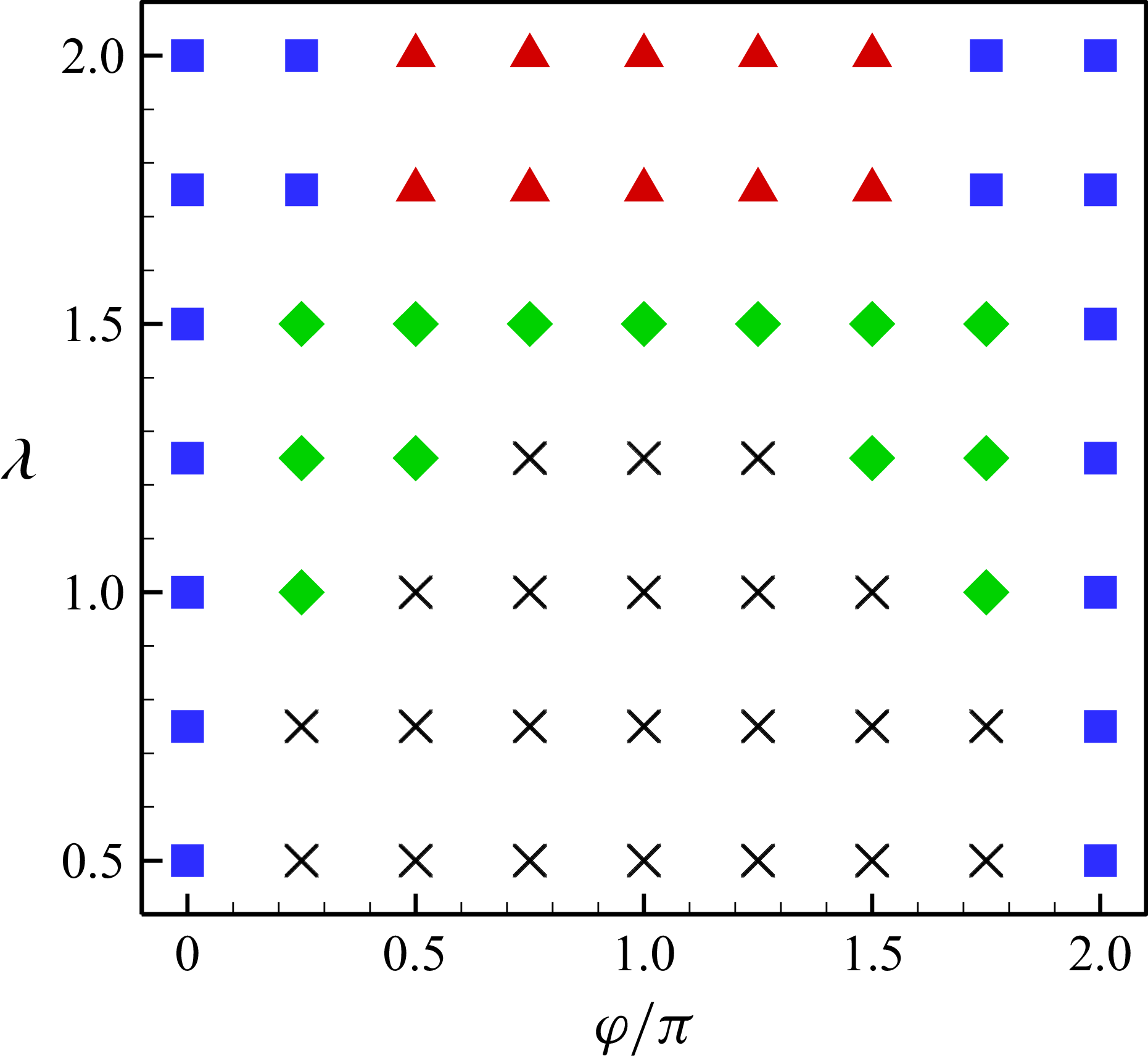
, respectively. In this study, a stable formation is defined as a state where the longitudinal and lateral distances between the two fish converge to constant values or fluctuate periodically. The results are illustrated in figure 3; it is interesting that two fish can self-organise into stable formations through the hydrodynamic interactions alone, without any control algorithm. Moreover, figure 3 shows that when two fish undulate in phase (i.e.
 $\varphi =0$
or
 $2\pi$
), a stable formation is maintained regardless of the wavelength. However, when two fish exhibit phase-shifted undulation (i.e.
 $0\lt \varphi \lt 2\pi$
), a large wavelength is essential for the emergence of stable formations. The threshold wavelength, above which stable formations can be achieved, increases as the absolute value of
 $\varphi -\pi$
(i.e.
 $|\varphi -\pi |$
) decreases. Furthermore, because of the inherent symmetry of phase difference, the values of
 $\bar{G}_x$
are equal in magnitude but opposite in sign for fixed
 $|\varphi -\pi |$
, but the values of
 $\bar{G}_y$
are identical. As a result, the stable formations exhibit symmetric distribution with respect to
 $\varphi =\pi$
, as shown in figure 3. The similar symmetry has also been reported for the hydrodynamic performance of two rigid pitching foils arranged in a side-by-side configuration (Dewey et al. Reference Dewey, Quinn, Boschitsch and Smits2014).
Values of the controlled parameters used in the current simulations.

The distribution of three distinct modes in the
 $\varphi{-}\lambda$
phase diagram. The blue square symbol represents the steady slow mode, the red triangle symbol represents the steady fast mode, the green diamond symbol represents the fluctuating fast mode, and the black cross symbol represents the unstable cases.

To investigate the characteristics of these modes, three typical cases, i.e.
 $\varphi =0, \lambda =1.0$
,
 $\varphi =\pi , \lambda =1.75$
and
 $\varphi =\pi , \lambda =1.5$
, are selected for analysis. As shown in figure 4(a), the lateral distances (
 $G_y$
) exhibit dramatic variations initially, and converge to a constant value or fluctuate periodically after approximately
 $200$
undulation cycles. Meanwhile, the longitudinal distances remain almost unchanged throughout the entire process. That is, the fish school achieves a stable formation after approximately
 $200$
cycles. Once a stable formation is established, two fish can maintain straight-line self-propulsion, with the yaw angle of each fish much smaller than
 $1^\circ$
. Specifically, the cycle-averaged lateral speed of each fish (of the order of
 $10^{-3}$
) is much smaller than its cycle-averaged longitudinal speed. Therefore, the stable formations can be classified into three distinct modes by comparing the cycle-averaged longitudinal speed of the fish school with that of an isolated fish. The steady slow mode (blue square symbol in figure 3) is defined as the case where the cycle-averaged longitudinal speed of the fish school is constant and smaller than that of an isolated fish. The steady fast mode (red triangle symbol in figure 3) is defined as the case where the cycle-averaged longitudinal speed of the fish school is constant but higher than that of the isolated fish. The fluctuating fast mode (green diamond symbol in figure 3) is defined as the case where the cycle-averaged longitudinal speed of the fish school fluctuates periodically, with its mean value over the fluctuation period
 $T^*$
(much larger than the undulation period
 $T$
) exceeding that of the isolated fish. On the other hand, figures 4(b) and 4(c) show that in both the steady slow and steady fast modes, the cycle-averaged lateral speed of each fish is approximately zero. Thus the two fish can maintain straight-line self-propulsion in these two modes, as shown in figure 4(e). In contrast, in the fluctuating fast mode, the cycle-averaged lateral speeds of the two fish fluctuate symmetrically about zero relative to each other, resulting in oscillatory trajectories, as shown in figure 4(f).
(a) Time histories of the separation distances between two fish in different cases. (b–d) The cycle-averaged speeds of the fish school respectively in the (b) steady slow mode, (c) steady fast mode, and (d) fluctuating fast mode. (e, f) The trajectories of two fish respectively in the cases (e)
 $\varphi =0, \lambda =1.0$
and (f)
 $\varphi =\pi , \lambda =1.5$
.

Moreover, figure 3 shows that the occurrence of each mode depends on phase difference and wavelength. The steady slow mode emerges only when
 $|\varphi -\pi | \geqslant 0.75\pi$
. That is, the small phase difference is necessary for the steady slow mode. Notably, the steady slow mode is unique to the in-phase fish school (i.e.
 $\varphi = 0$
or
 $2\pi$
). Furthermore, the steady fast mode occurs under the conditions
 $| \varphi -\pi | \leqslant 0.5\pi$
and
 $\lambda \geqslant 1.75$
. In contrast, the fluctuating fast mode emerges when
 $| \varphi - \pi | \leqslant 0.75\pi$
and
 $\lambda \leqslant 1.5$
. For a fixed phase difference, the wavelength of fish in the fluctuating fast mode is smaller than that in the steady fast and slow modes. Furthermore, inter-fish collision occurs when the wavelength is sufficiently small, as indicated by the black cross symbol in figure 3. Compared with the previous study (Lin et al. Reference Lin, Wu, Zhang and Yang2021), the results here demonstrate that the self-organisation behaviour of the fish school becomes more complex under the influence of wavelength and phase difference.
In addition, it should be pointed out that when
 $\lambda \gg 1$
, the collective locomotion of the fish school is similar to that of rigid foils. Dewey et al. (Reference Dewey, Quinn, Boschitsch and Smits2014) revealed that compared with a single pitching foil, two rigid foils arranged in the side-by-side formation exhibit thrust reduction when
 $\varphi \leqslant \pi /8$
or
 $\varphi \geqslant 15\pi /8$
, but thrust enhancement when
 $\pi /8 \lt \varphi \lt 15\pi /8$
. As shown in figure 3, when
 $\lambda \geqslant 1.75$
, both the steady slow and fast modes, as well as their phase ranges, are consistent with the performance of two rigid pitching foils fixed in the uniform incoming flow. On the other hand, considering the self-propulsion of rigid foils, the phase range for the steady fast mode is close to that required for two rigid foils to achieve a stable side-by-side formation (Newbolt et al. Reference Newbolt, Zhang and Ristroph2022). In addition, the emergence of the steady slow mode demonstrates that maintaining a stable side-by-side formation can lead to a speed reduction for the in-phase fish school. Similarly, such a speed reduction has been observed for two burst-and-coast pitching foils (Chao, Bhalla & Li Reference Chao, Bhalla and Li2023; Jin, Wang & Deng Reference Jin, Wang and Deng2025).
The cycle-averaged (a) longitudinal and (b) lateral distance as a function of wavelength and phase difference. (c) The distribution of the three distinct modes in the
 $\bar{G}_x{-}\bar{G}_y$
phase diagram, where
 $\bar{G}_x$
and
 $\bar{G}_y$
in the fluctuating fast mode are calculated over the fluctuating period
 $T^*$
. (d) The cycle-averaged swimming speed of the fish school as a function of
 $\bar{G}_y$
.

To further analyse the formation characteristics in different modes, the cycle-averaged longitudinal spacing (
 $\bar{G}_x$
) and lateral spacing (
 $\bar{G}_y$
) between two fish are calculated and illustrated in figures 5(a) and 5(b). It can be seen that when
 $\varphi =0-\pi$
,
 $\bar{G}_x$
varies only within a narrow range
 $0{-}0.1$
across different parameters, while
 $\bar{G}_y$
increases significantly from
 $0.4$
to
 $1.0$
with the rise of
 $\lambda$
and
 $\varphi$
. It is clear that
 $\bar{G}_y$
is sensitive to
 $\lambda$
, but
 $\bar{G}_x$
is almost unaffected. The reason may be that the inter-body interaction between two fish, which determines
 $\bar{G}_y$
, strongly depends on
 $\lambda$
, whereas the wake vortex distribution that restores
 $\bar{G}_x$
is insensitive to
 $\lambda$
(Ormonde et al. Reference Ormonde, Kurt, Mivehchi and Moored2024). Moreover, some overlapping symbols can be observed in figure 5(c), which indicates that the same formation can be achieved by the fish school with different parameters. The reason may be that there exists a coupling effect between phase difference and wavelength on the emergence of stable formations. In addition, observations of living fish schools have shown that
 $\bar{G}_x$
typically varies within a range of approximately
 $0.1{-}0.2$
, while
 $\bar{G}_y$
is approximately
 $0.5{-}0.7$
(Ashraf et al. Reference Ashraf, Godoy-Diana, Halloy, Collignon and Thiria2016). The discrepancy in
 $\bar{G}_x$
between the present and experimental results may be due to the neglect of the lateral line perception system. However, the values of
 $\bar{G}_y$
are in general agreement with experimental results (Ashraf et al. Reference Ashraf, Godoy-Diana, Halloy, Collignon and Thiria2016).
On the other hand, as shown in figure 5(c),
 $\bar{G}_y$
gets its minimum value in the steady slow mode, but maximum value in the steady fast mode. This indicates that fish schools with greater lateral spacing swim faster than those with smaller lateral spacing. As shown in figure 5(d), it is clear that the swimming speed of fish school increases with
 $\bar{G}_y$
. This is counterintuitive, since previous studies (Ambolkar & Arumuru Reference Ambolkar and Arumuru2022; Jeong et al. Reference Jeong, Kim and Lee2023) have reported that swimming speed decreases with increasing lateral distance. However, it is consistent with the previous experimental results (Ashraf et al. Reference Ashraf, Godoy-Diana, Halloy, Collignon and Thiria2016), in which the swimming speed of fish school increases with the lateral spacing. The reason why the collective speed increases with
 $\bar{G}_y$
can be explained as follows. For the fixed kinematic parameters (including the wavelength, frequency and amplitude), the wake deflection angle of the fish school decreases with the rise of
 $\bar{G}_y$
. The smaller wake deflection angle implies less lateral dissipation of the jet flow, which in turn enhances the thrust of the fish school and thereby increases its swimming speed. The relationship between the wake deflection angle and the performance of the fish school will be discussed in detail in the next subsection.
(a) The Strouhal number as a function of the wavelength. (b) The equilibrium lateral distance, (c) power consumption and (d) cost of transport of the fish school as functions of the Strouhal number.

The Strouhal number (
 $St$
) is one of the important quantities used to describe fish swimming, defined as
 $St=2fA/\bar{u}_x$
. As shown in figure 6(a), the values of
 $St$
range from
 $0.74$
to
 $1.15$
. Although the interval
 $0.2{-}0.4$
is widely considered as the optimal
 $St$
range for most fish species (Taylor, Nudds & Thomas Reference Taylor, Nudds and Thomas2003), the values of
 $St$
observed in real fish schools exhibit a wide variation (Santo et al. Reference Di Santo, Goerig, Wainwright, Akanyeti, Liao, Castro-Santos and Lauder2021). For instance,
 $St$
of the red-nose tetra fish group ranges from
 $0.2$
to
 $1.5$
during collective swimming (Ashraf et al. Reference Ashraf, Godoy-Diana, Halloy, Collignon and Thiria2016, Reference Ashraf, Bradshaw, Ha, Halloy, Godoy-Diana and Thiria2017). Consequently, the values of
 $St\ (=0.74{-}1.15)$
obtained here are still consistent with the observations of real fish schools. In addition, as shown in figure 6(b),
 $\bar{G}_y$
decreases with the rise of
 $St$
, since
 $\bar{u}_x$
increases with
 $\bar{G}_y$
while
 $\textit{fA}$
is constant. This is different from the results in previous studies (Kurt et al. Reference Kurt, Cochran-Carney, Zhong, Mivehchi and Quinn2019; Ormonde et al. Reference Ormonde, Kurt, Mivehchi and Moored2024), in which the lateral movement of a flapping foil was constrained. Moreover, as shown in figure 6(c), the power consumption of the fish school decreases significantly with the rise of
 $St$
. Consequently, as
 $St$
increases, the variation of
 $\textit{CoT}$
depends on the wavelength. As shown in figure 6(d), when
 $\lambda =1.25$
,
 $\textit{CoT}/\textit{CoT}_s$
increases with
 $St$
. That is, the efficiency advantage of the fish school decreases with increasing
 $St$
when
 $\lambda$
is small. When
 $\lambda =1.5$
and
 $1.75$
,
 $\textit{CoT}/\textit{CoT}_s$
decreases first and then increases with
 $St$
. However, when
 $\lambda =2$
,
 $\textit{CoT}/\textit{CoT}_s$
decreases significantly as
 $St$
increases. This indicates that the efficiency of the fish school increases with
 $St$
when
 $\lambda$
is large enough.
3.2. Collective performance in the steady slow mode
The cycle-averaged speed, power consumption and cost of transport of the fish school in the steady slow mode are calculated and compared with those of a single fish. As shown in figure 7(a), it is clear that the swimming speed of the fish school in this mode is smaller than that of a single fish. The speed reduction is affected by both wavelength and phase difference, and a maximum reduction of 6 % occurs in the case
 $\varphi =0, \lambda =2.0$
. However, the power consumption of the fish school is also smaller than that of an isolated fish; the maximum reduction reaches approximately 9 % in the case
 $\varphi =0, \lambda =1.75$
. This means that a fish school in the steady slow mode has energy saving, although its swimming speed is decreased. Consequently,
 $\textit{CoT}$
of the fish school is smaller than that of a single fish; the maximum reduction 7 % can be obtained in the cases
 $\varphi =0.25\pi, 1.75\pi ,\ \lambda =1.75$
. Consequently, a fish school in the steady slow mode has higher efficiency than an isolated fish.
The relative differences in cycle-averaged speed, power consumption and the cost of transport for (a) fish school, (b) fish 1 and (c) fish 2. The subscripts 1, 2 and
 $s$
respectively represent fish 1, fish 2 and single fish, as in the text.

As for each fish in the school, significant energy savings are observed in all cases except the case
 $\varphi =2\pi , \lambda =2$
, as shown in figures 7(b) and 7(c). Moreover, when two fish swim synchronously (
 $\varphi =0$
or
 $2\pi$
), the differences in energy consumption and efficiency between them are negligible. Especially when
 $\lambda \geqslant 1.0$
, each fish has energy saving above
 $8{-}10\,\%$
. However, when
 $\varphi =0.25\pi$
, fish 1 achieves significant energy savings, whereas fish 2 does not. It should be pointed out that the performance of fish 1 in the case
 $\varphi =1.75\pi$
is consistent with that of fish 2 in the case
 $\varphi =0.25\pi$
. Meanwhile, fish 2 in the case
 $\varphi =1.75\pi$
performs like fish 1 in the case
 $\varphi =0.25\pi$
. Therefore, for two asynchronous fish in the steady slow mode, the group’s energy saving primarily results from one individual. Additionally, it should be pointed out that the performances of fish 1 and fish 2 are diametrically reversed for a fixed value of
 $|\varphi -\pi |$
when
 $\varphi \gt \pi$
. This is the reason why the performance of fish 1 and fish 2 has not been illustrated when
 $\varphi \gt \pi$
, and similarly in the following subsections.
To further investigate the performance of a fish school in the steady slow mode, the case
 $\varphi =0, \lambda =2$
, in which the maximum speed reduction occurs, is selected as the typical case for analysis. As shown in figure 8(a), in the steady slow mode, the swimming speeds of both fish are always lower than the speed of a single fish. Additionally, each fish has two speed peaks of different magnitudes in one cycle. For example, fish 1 has a higher speed peak at
 $0.15T$
as compared to that at
 $0.65T$
, while fish 2 shows the opposite trend. This is mainly attributed to the presence of two distinct thrust peaks with different magnitudes for both fish, as shown in figure 8(b). The different thrust peaks of each fish in one cycle result from the differential pressure distributions around their heads, which are induced by the lateral interface between them. As shown in figure 8(c), at
 $t/T=0.5$
, a positive pressure region exists on the right anterior side of each fish (the right side is defined as the side with a larger
 $y$
-coordinate compared to the left side), which is bad for thrust generation, as shown by the black arrows F1 and F3. In addition, a negative pressure region appears on the left anterior side of each fish, which is good for thrust generation, as shown by the black arrows F2 and F4. Furthermore, the positive pressure region on the right anterior side of fish 1 is stronger than that for fish 2, but the negative pressure region on the left anterior side of fish 2 is stronger than that for fish 1. As a result, the thrust of fish 1 is smaller than that of fish 2 at
 $t/T=0.5$
, as shown in figure 8(b). However, at
 $t/T=1.0$
, the negative pressure region on the right anterior side of fish 1 is stronger than that for fish 2, but the positive pressure region on the left anterior side of fish 2 is stronger than that for fish 1, as shown in figure 8(d). Consequently, the thrust of fish 1 is larger than that of fish 2 at this moment, as shown in figure 8(b).
Time histories of (a) the swimming speed and (b) the thrust coefficient of each fish in a school and an isolated fish. (c,d) Instantaneous pressure coefficient contours of the fish school at
 $t/T$
values (c) 0.5 and (d) 1.0 in the case
 $\varphi =0, \lambda =2$
. The arrows F1–F4 in (c) represent the approximate directions of the push or suction effects generated by the flow, and the same holds for the arrows in figures 13 and 17.

On the other hand, the different thrust peaks of each fish in one period are always associated with its wake deflection (Gungor, Khalid & Hemmati Reference Gungor, Khalid and Hemmati2022). As shown in figure 9(a), it is clear that the wake of each fish is obviously deflected outwards. To explore the mechanism of wake deflection, the effective phase velocities of the two consecutive dipoles are calculated (Godoy-Diana et al. Reference Godoy-Diana, Marais, Aider and Wesfreid2009; Zheng & Wei Reference Zheng and Wei2012). As shown in figure 9(b), dipole 1 is formed by vortices V1 and V2, and dipole 2 is formed by vortices V2 and V3. The effective phase velocity of each dipole is calculated as
 $U^*=U_d-U_p \cos\alpha$
, where
 $U_p$
(the yellow arrows) is the average streamwise velocity of the two vortex centres of a dipole,
 $\alpha$
is the orientation angle between the streamwise direction and the direction of the dipole,
 $U_d$
(
 $=\varGamma /(2\pi \xi )$
, the black arrows) is the dipole induced velocity,
 $\xi$
is the distance between two vortices, and
 $\varGamma$
is the averaged circulation of two vortices in the dipole. For the case here, as shown in figure 9(b), the effective phase velocity of dipole 1 (
 $U_1^*=0.22$
) is much larger than that of dipole 2 (
 $U_2^*=0.14$
). Therefore, the wake of fish 1 deflects outwards along
 $U_1^*$
. This is consistent with previous studies (Zheng & Wei Reference Zheng and Wei2012; Zhu et al. Reference Zhu, He and Zhang2014b
; Wu et al. Reference Wu, Shu, Wan, Wang and Chen2022b
).
(a) Instantaneous vorticity at
 $t/T=0.25$
. (b) A schematic illustration of two consecutive dipoles. (c) The time-averaged longitudinal velocity field of the fish school. (d) The velocity profile at
 $x/L=1.0$
in the case
 $\varphi =0, \lambda =2$
.

Moreover, the wake structure of the fish school is the same as that of a single fish, i.e. the 2S reversed von Kármán vortex street. To further investigate the speed varaition of the fish school, the time-averaged longitudinal velocity field of the fish school is calculated. A rectangular domain (
 $\varOmega$
) of
 $8c \times 4c$
is defined, which moves synchronously with the fish 1, as indicated by the green dash-dotted region in figure 9(a). The time-averaged longitudinal velocity is calculated by averaging the longitudinal speed of flow in the region
 $\varOmega$
in one period. For comparison, the time-averaged longitudinal velocity field of a single fish is calculated. As shown in figures 9(c) and 9(d), there exists a jet flow behind each fish, which is consistent with the 2S reversed von Kármán vortex street. Moreover, several previous studies (Peng et al. Reference Peng, Huang and Lu2018; Wu et al. Reference Wu, Shu, Lee and Wan2022a
) revealed that for the same wake vortex structure, the strength of the wake jet is strongly correlated with the propulsive speed, i.e. a stronger jet indicates greater thrust and thus higher propulsion speed. As shown in figures 9(c) and 9(d), the strength of jet flow of the fish school is obviously weaker than that of a single fish. Morevoer, the jet flow of each fish is deflected, which also inhibits its thrust generation. As a result, the fish school swims more slowly than a single fish in this mode.
In order to investigate the relationship between the wake deflection and the collective performance of the fish school, the wake deflection angle (
 $\beta$
, as shown in figure 9(c)) is calculated for each case in the steady slow mode. As shown in figure 10(a),
 $\beta$
increases with
 $\lambda$
when
 $\lambda \leqslant 1.25$
, whereas it decreases with the rise of
 $\lambda$
when
 $\lambda \gt 1.25$
. Moreover, as shown in figure 10(b), the swimming speed difference between the fish school and a single fish decreases with the rise of
 $\beta$
when
 $\lambda \leqslant 1.25$
, but increases with
 $\beta$
when
 $\lambda \gt 1.25$
. However, the power consumption difference between the fish school and an isolated fish is negative, and its magnitude increases with the rise of
 $\beta$
, and the same trend is observed for the difference of
 $\textit{CoT}$
, as shown in figures 10(c) and 10(d). Taken together, in the steady slow mode, the collective performance of the fish school becomes more economical and efficient as
 $\beta$
increases.
(a) The wake deflection angle of the fish school as a function of wavelength. The relative differences in time-averaged (b) swimming speed, (c) power consumption, (d) cost of transport as functions of the wake deflection angle.

3.3. Collective performance in the steady fast mode
In the steady fast mode, although the fish school swims faster than a single fish, the speed enhancement is significantly affected by both wavelength and phase difference. As shown in figure 11(a), the fish school achieves a higher swimming speed at
 $\lambda =1.75$
than at
 $\lambda =2.0$
. Moreover, the speed enhancement increases as
 $|\varphi - \pi |$
decreases, reaching the maximum at
 $\varphi =\pi$
. The maximum speed enhancement is approximately
 $7\,\%$
, which occurs in the case
 $\varphi =\pi , \lambda =1.75$
. However, the fish school exhibits no significant energy saving in this mode, except in the cases
 $\varphi =0.5\pi, 1.5\pi ,\ \lambda =1.75$
. Consequently, as compared with a single fish, the fish school has a significant efficiency advantage at
 $\lambda =1.75$
, but it disappears at
 $\lambda =2.0$
. This indicates that shorter wavelengths are more favourable for the fish school in the steady fast mode.
Moreover, as shown in figures 11(b) and 11(c), fish 1 achieves energy savings in some cases (such as
 $\varphi =0.5\pi$
), with the maximum energy saving of up to
 $9\,\%$
observed in the case
 $\varphi =0.5\pi , \lambda =1.75$
. Furthermore, fish 1 has the efficiency advantage in most cases, and the maximum reduction of
 $\textit{CoT}$
reaches
 $12\,\%$
in the case
 $\varphi =0.5\pi , \lambda =1.75$
. However, fish 2 requires more power consumption in all of the cases, and has no efficiency advantage, except in the cases
 $\varphi =0.75\pi, \pi ,\ \lambda =1.75$
. Additionally, the performances of fish 1 and fish 2 are diametrically reversed for a fixed value of
 $|\varphi -\pi |$
when
 $\varphi \gt \pi$
.
The relative differences in cycle-averaged speed, power consumption and the cost of transport between fish in steady fast mode and in solitary swimming: (a) fish school, (b) fish 1 and (c) fish 2.

Time histories of (a) the swimming speed and (b) the thrust coefficient of each fish in the steady slow mode and solitary swimming.

Similarly, the case
 $\varphi =1.0\pi , \lambda =1.75$
, in which the maximum speed enhancement is achieved, is selected as the typical case for analysis. As shown in figure 12(a), the propulsive speed of the fish school consistently exceeds that of a single fish throughout the entire cycle in the steady fast mode. Moreover, the speed has two peaks with different magnitudes in one cycle. This is because the thrust of each fish has two distinct peaks with varying amplitudes. As shown in figure 12(b), the thrust of each fish in the school is smaller than that of an isolated fish at
 $t/T=0$
and
 $1.0$
, but larger at
 $t/T=0.5$
. The thrust difference between the fish school and a single fish primarily results from the lateral interactions between individuals, which can be described as follows.
Instantaneous pressure coefficient contours of (a,b) the fish school and (c) a single fish. (d) Instantaneous vorticity and (e) time-averaged longitudinal velocity field of the fish school. (f) The velocity profile at
 $x/L=1.0$
in the case
 $\varphi =\pi , \lambda =1.75$
.

As shown in figures 13(a–c), it is clear that the pressure on the left side of fish 1 is significantly stronger than that of a single fish at
 $t/T=0.5$
. Moreover, the negative pressure acting on the left anterior side has a suction effect on fish 1 (as indicated by arrow F1), while the positive pressure on the left posterior side generates a push effect on fish 1 (as indicated by arrow F2). Both the suction and push effects are beneficial to the thrust generation of fish 1, thus the thrust of fish 1 is larger than that of a single fish at
 $t/T=0.5$
. However, at the moment
 $t/T=1.0$
, although the pressure on the left side of fish 1 remains significantly stronger than that of a single fish, the positive pressure acting on the left front region generates a push effect on fish 1 (as indicated by arrow F3), which is detrimental to thrust generation. Therefore, the thrust of fish 1 is smaller than that of a single fish at
 $t/T=1.0$
. Furthermore, a similar lateral interaction occurs for fish 2, as shown in figures 13(a) and 13(b). This is the reason why the thrust of each fish has two distinct peaks of varying amplitudes.
On the other hand, the instantaneous vorticity contours of the fish school in the steady fast mode are illustrated in figure 13(d); it is clear that the wake of each fish deflects outwards. As a result, the jet flow behind each fish is deflected, as shown in figure 13(e). Moreover, as compared with a single fish, the strength of the wake jet of each fish in the school is obviously stronger, as shown in figure 13(f). Consequently, the fish school swims faster than an isolated fish in this mode. Furthermore, as shown in figure 14(a), it is clear that
 $\beta$
decreases with the rise of
 $\bar{G}_y$
, which is consistent with previous studies (Dai et al. Reference Dai, He, Zhang and Zhang2018; Kurt et al. Reference Kurt, Cochran-Carney, Zhong, Mivehchi and Quinn2019). Moreover, as
 $\beta$
increases, the speed enhancement of the fish school decreases dramatically, and the same trend is observed for their power consumption, as shown in figures 14(b) and 14(c). As a result, the cost of transport of the fish school decreases slightly with increasing
 $\beta$
, as shown in figure 14(d). Therefore, for the fish school in the steady fast mode, an increased wake deflection angle can lead to a dramatic reduction in energy consumption and a slight increase in efficiency, at the cost of decreased swimming speed.
(a) The wake deflection angle of the fish school as a function of lateral equilibrium distance. The relative differences in time-averaged (b) swimming speed, (c) power consumption, (d) cost of transport as functions of wake deflection angle.

3.4. Collective performance in the fluctuating fast mode
In the fluctuating fast mode, although the swimming speed of the fish school oscillates with the primary undulating cycle, its magnitude is modulated by a much larger-period oscillation. The criterion for determining the convergence of the fluctuating fast modes is that the maximum and minimum values of
 $G_x$
and
 $G_y$
, as well as the fluctuating period (
 $T^*$
), remain constant. As shown in figures 15(a) and 15(b), the cycle-averaged longitudinal and lateral speeds fluctuate with a period that is much larger than the undulation period. Moreover, it can be seen from figure 15(a) that the cycle-averaged longitudinal speeds over the undulation periods of fish 1 and fish 2 do not match each other when
 $|\varphi -\pi | \neq 0$
. Thus the longitudinal spacing (
 $G_x$
) oscillates when
 $|\varphi -\pi | \neq 0$
, as shown in figure 15(c). The oscillation amplitude (
 $A_x$
) of longitudinal spacing has been calculated, as illustrated in figure 15(d). It is clear that as
 $\varphi$
increases,
 $A_x$
decreases until reaching its minimum value (approximately 0) at
 $\varphi = \pi$
, then increases thereafter. This indicates that the difference in longitudinal speeds between two fish increases with
 $|\varphi -\pi |$
. Furthermore, the variations of the cycle-averaged lateral speeds of fish 1 and 2 are opposite, as shown in figure 15(b). As a result, the lateral spacing (
 $G_y$
) undergoes oscillation, as shown in figure 15(c). The oscillating amplitude (
 $A_y$
) of lateral spacing is illustrated in figure 15(e); it is clear that
 $A_y$
is larger than
 $A_x$
. On the other hand, the value of
 $T^*$
is calculated as shown in figure 15(f), and it is clear that the fluctuating period is much larger than the undulation period. Moreover, the fluctuating period increases with the reduction of
 $|\varphi -\pi |$
.
Consequently, in the fluctuating fast mode, the time-averaged speed and power consumption of each fish are calculated over the fluctuating period, and the results are illustrated in figure 16. It can be seen from figure 16(a) that for a fixed wavelength (e.g.
 $\lambda =1.5$
), the swimming speed of the fish school increases significantly as
 $|\varphi -\pi |$
decreases. The maximum speed enhancement (more than
 $12\,\%$
) is achieved by the group in the case
 $\varphi =\pi , \lambda =1.5$
. Moreover, the fish school has energy saving in the cases
 $|\varphi -\pi |=0.75\pi$
, but requires more power consumption in the other cases. However,
 $\textit{CoT}$
of the fish school is smaller than that of an isolated fish in all cases here. That is, both the swimming efficiency and speed of the fish school outperform those of an isolated fish in this mode. However, it should be pointed out that the performance improvement of the fish school in this study is significantly weaker than that reported in previous studies (Dewey et al. Reference Dewey, Quinn, Boschitsch and Smits2014; Peng et al. Reference Peng, Huang and Lu2018; Newbolt et al. Reference Newbolt, Zhang and Ristroph2022). This is because the lateral recoil oscillation, which was neglected in previous studies (Dewey et al. Reference Dewey, Quinn, Boschitsch and Smits2014; Peng et al. Reference Peng, Huang and Lu2018; Newbolt et al. Reference Newbolt, Zhang and Ristroph2022), can significantly weaken the ground effect between two parallel fish, thereby reducing the performance improvement (Kurt et al. Reference Kurt, Cochran-Carney, Zhong, Mivehchi and Quinn2019). Furthermore, the similar modest performance enhancement has also been observed in the collective propulsion of two rigid pitching foils (Ormonde et al. Reference Ormonde, Kurt, Mivehchi and Moored2024) and a rigid pitching foil swimming freely near the ground (Kurt et al. Reference Kurt, Cochran-Carney, Zhong, Mivehchi and Quinn2019).
As for each fish in the fluctuating fast mode, as shown in figure 16(b), fish 1 generally consumes less power when
 $\varphi =0.25\pi{-}\pi$
, except in the case
 $\varphi =\pi , \lambda =1.5$
. Specifically, the energy saving of fish 1 exceeds
 $10\,\%$
when
 $\varphi =0.25\pi$
. Consequently, the
 $\textit{CoT}$
of fish 1 is much smaller than that of a single fish, with the maximum reduction exceeding
 $15\,\%$
. That is, fish 1 has a significant efficiency advantage in this mode. In contrast, fish 2 generally consumes much more power in this mode when
 $\varphi =0.25\pi{-}\pi$
, as shown in figure 16(c). That is, fish 2 has no obvious energy advantage. Moreover, the
 $\textit{CoT}$
of fish 2 is also larger than that of a single fish in most cases. Consequently, the efficiency and energy advantages of the fish school in the fluctuating fast mode are mainly attributed to energy saving of one individual, such as fish 1 in the cases
 $\varphi = 0.25\pi{-}\pi$
.
The cycle-averaged (a) longitudinal speed and (b) lateral speed of the fish school. (c) Time histories of the separation distances between two fish. The oscillation amplitudes of (d) longitudinal and (e) lateral spacings, and (f) the fluctuating period as a function of phase difference.

The relative differences in cycle-averaged speed, power consumption and the cost of transport between fish in fluctuating fast mode and values in solitary swimming: (a) fish school, (b) fish 1 and (c) fish 2.

To further investigate the performance of the fish school in the fluctuating fast mode, the case
 $\varphi =\pi , \lambda =1.5$
with interval
 $t/T=220{-}221$
is selected for analysis. As shown in figure 17(a), it is clear that the speed of the fish school is larger than that of a single fish throughout the entire interval, with two peaks of differing magnitudes observed. This phenomenon arises because the thrust curves of the fish school also exhibit two peaks with distinct magnitudes, as shown in figure 17(b). Moreover, it can be seen from figures 17(c) and 17(d) that the lateral interface induces a high positive pressure on the left anterior side of fish at
 $t/T=0.2$
, but a negative pressure at
 $t/T=0.7$
. The positive pressure exerts a push effect (as shown by arrow F1) on the fish, while the negative pressure creates a suction effect (as shown by arrow F2). Thus the thrust of each fish in the school is smaller than that of an isolated fish at
 $t/T=0.2$
, but greater at
 $t/T=0.7$
, as shown in figure 17(b).
On the other hand, the instantaneous vorticity contours of the fish school are illustrated in figures 18(a) and 18(b). Similar to the steady slow and fast modes, the wake of each fish is deflected outwards. Moreover, as shown in figures 18(c) and 18(d), it is clear that the strength of the wake jet of the fish school is obviously stronger than that of a single fish. Thus the fish school swims faster than a single fish in this mode. It should be pointed out that only the 2S reversed von Kármán vortex street is observed in the present study; the complex merged wake patterns are absent, which have been observed for two parallel foils fixed in the uniform incoming flow or self-propelled along the longitudinal direction (Dewey et al. Reference Dewey, Quinn, Boschitsch and Smits2014; Peng et al. Reference Peng, Huang and Lu2018; Gungor et al. Reference Gungor, Khalid and Hemmati2022; Chao et al. Reference Chao, Bhalla and Li2023). This indicates that the lateral flow-mediated organisation between two fish can avoid the complex vortex patterns.
Time histories of (a) the swimming speed and (b) the thrust coefficient. (c,d) Instantaneous pressure coefficient contours of the fish school in the fluctuating fast mode.

(a,b) Instantaneous vorticity contours of the fish school in the fluctuating fast mode. (c) The time-averaged longitudinal velocity fields of fish school. (d) The velocity profile at
 $x/L=1.0$
in the case
 $\varphi =\pi , \lambda =1.5$
.

3.5. The mechanism behind stable formations
In the present study, the cycle-averaged longitudinal spacings between two fish in the stable formations vary only within a narrow range regardless of the dynamic modes, as shown in figure 5(c). That is, all stable formations approximate the side-by-side configurations. Similar behaviour has been observed for two rigid anti-phase pitching foils (Lin et al. Reference Lin, Wu, Zhang and Yang2021; Ormonde et al. Reference Ormonde, Kurt, Mivehchi and Moored2024). Moreover, the emergence of these stable formations indicates that two fish can achieve equilibrium positions simultaneously in both the longitudinal and lateral directions. In this subsection, we will investigate the hydrodynamic mechanisms by which the fish school maintains its equilibrium longitudinal and lateral positions.
The reason why two fish maintain almost zero longitudinal distance can be explained as follows. When the longitudinal separation between two fish becomes large due to the perturbation, the trailling edge vortex shed from the leader can generate a push effect on the follower, which enhances the follower’s thrust, thereby increasing its speed and decreasing the longitudinal distance until the equilibrium position is restored. To validate the hypothesis, the performance of two fish with a large longitudinal distance has been simulated. In this simulation, two fish are fixed in the uniform flow in which the incoming speed equals the time-averaged speed of the fish school with the same kinematics, and the control parameters are
 $\varphi =0,\ \lambda =1.25,\ G_x=-0.3,\ G_y=0.5$
. As shown in figure 19, in contrast to the symmetric wake vortex distribution behind the two fish in a stable formation, the wake vortex distribution becomes asymmetric when the longitudinal separation increases. When fish 2 is positioned downstream of fish 1, the clockwise vortex (e.g. V1) shed from the trailing edge of fish 1 is relatively close to fish 2. Thus this clockwise vortex can induce the flow towards fish 2, generating a push effect (as shown by the green arrow) on fish 2 and increasing its thrust. As shown in figure 20(a), the thrust of fish 2 (
 $\bar{C}_{T\_{fish 2}}=0.37$
) is obviously larger than that of fish 1 (
 $\bar{C}_{T\_{fish 1}}=0.26$
). Such larger thrust allows fish 2 to increase its speed and catch up with fish 1.
Instantaneous vorticity of (a) two fish fixed in the uniform incoming flow and (b) two self-propelled fish.

(a) Time histories of thrust coefficients of two fish fixed in the uniform incoming flow in the case
 $\varphi =0,\ \lambda =1.25,\ G_x=-0.3,\ G_y=0.5$
. (b–d) The cycle-averaged lateral force coefficients of two fish arranged in the side-by-side formation as functions of the lateral spacing, where the control parameters are (b)
 $\varphi =0, \lambda =2.0$
, (c)
 $\varphi =\pi , \lambda =1.75$
, (d)
 $\varphi =\pi , \lambda =1.5$
.

In order to investigate the mechanism underlying the equilibrium lateral positions, the performance of two fish arranged in the side-by-side formation with different lateral distances has been simulated. The cases
 $\varphi =0, \lambda =2.0$
,
 $\varphi =\pi , \lambda =1.75$
and
 $\varphi =\pi,{} \lambda =1.5$
, respectively, are selected as examples of the steady slow mode, steady fast mode and fluctuating fast mode. As shown in figures 20(b) and 20(c), in the cases
 $\varphi =0, \lambda =2.0$
and
 $\varphi =\pi , \lambda =1.75$
, it is clear that the lateral force acting on each fish is non-zero when the lateral distance between the two fish is close to the equilibrium position. Moreover, the lateral force on fish 1 is positive, whereas that on fish 2 is negative, and the magnitude of the cycle-averaged lateral force on each fish decreases monotonically with increasing lateral distance. This indicates that in the steady slow mode and steady fast mode, the lateral forces generated by the inter-body interactions tend to push the two fish away from each other, and a stable formation is obtained when these lateral forces are balanced by the wake-deflection-induced forces (Kurt et al. Reference Kurt, Cochran-Carney, Zhong, Mivehchi and Quinn2019; Ormonde et al. Reference Ormonde, Kurt, Mivehchi and Moored2024).
Moreover, in the case
 $\varphi =\pi , \lambda =1.5$
, it is interesting to note that the cycle-averaged lateral forces acting on the two fish are approximately zero when the lateral distance between them is close to the equilibrium lateral position, as shown in figure 20(d). Moreover, the cycle-averaged lateral force acting on fish 1 changes from positive to negative, while that on fish 2 shifts from negative to positive, as the lateral distance increases near the equilibrium position. This indicates that the equilibrium lateral position in the fluctuating fast mode lies approximately at a critically stable equilibrium point, where the ground effect between two parallel fish switches from positive to negative. When the lateral spacing between the two fish is larger than the equilibrium value, a negative ground effect occurs, generating a lateral attractive force that pulls them closer and thus reduces the lateral spacing. In contrast, when the lateral spacing is smaller than the equilibrium value, a positive ground effect arises, producing a lateral repulsive force that pushes them apart and thereby increases the lateral spacing. This dynamic feedback between the lateral forces and the lateral spacing acts repeatedly on the two fish, ultimately resulting in the fluctuating fast mode.
4. Conclusions
In this paper, the impact of wavelength and phase difference on the flow-mediated schooling behaviour of two parallel fish is studied numerically. It is found that the two fish can simultaneously achieve equilibrium positions in both the longitudinal and lateral directions only via the hydrodynamic interactions, without any external control algorithm. In these stable formations, the cycle-averaged longitudinal spacing between two fish remains within
 $0{-}0.1$
, while the cycle-averaged lateral spacing increases from
 $0.4$
to
 $1.0$
with increasing
 $\lambda$
and
 $\varphi$
. Moreover, the swimming speed of fish schools increases with the cycle-averaged lateral spacing. Based on the cycle-averaged longitudinal speed of the fish school, the stable formations can be classified into three distinct modes, i.e. the steady slow mode, the steady fast mode and the fluctuating fast mode. Which mode occurs depends on the wavelength and phase difference. The steady slow mode is unique to the synchronous fish school (i.e.
 $\varphi =0$
and
 $2\pi$
), and it also arises when
 $|\varphi -\pi | \geqslant 0.75\pi$
with a sufficiently large wavelength (
 $\lambda \geqslant 1.75$
). Moreover, the steady fast mode occurs under the conditions
 $|\varphi -\pi | \leqslant 0.5\pi$
and
 $\lambda \geqslant 1.75$
, while the fluctuating fast mode emerges when
 $|\varphi -\pi | \leqslant 0.75\pi$
and
 $\lambda \leqslant 1.5$
.
In the steady slow mode, the fish school swims slower than a single fish, with maximum speed reduction
 $6\,\%$
, while its power consumption is significantly reduced by up to
 $9\,\%$
. Consequently, the fish school maintains higher propulsive efficiency than a single fish in the steady slow mode. In the steady fast mode, the fish school swims faster than a single fish, achieving maximum speed increase
 $7\,\%$
, but the significant efficiency advantage is only observed at
 $\lambda = 1.75$
. In the fluctuating fast mode, the fish school achieves speed enhancements exceeding
 $12\,\%$
, and exhibits a notable efficiency advantage across all cases, even though the power consumption is higher in some instances. Finally, the mechanism behind the stable formations has been analysed. The longitudinal stability is maintained by the restoring effect of the school’s wake, and the lateral stability results from the balance between lateral forces generated by the inter-body interactions and wake deflection. On the other hand, the emergence of the fluctuating fast mode is attributed to the presence of a critically stable equilibrium point in the lateral direction. The results obtained here can shed some light on understanding the collective motion of fish schools. Additionally, it should be pointed out that the model used in this study is highly simplified. Specifically, the influences of three-dimensional effects, Reynolds number and group size on fish schooling behaviour are just neglected here, and will be considered in future work.
Acknowledgements
X.L. acknowledges the financial support provided by the National Natural Science Foundation of China, the Natural Science Foundation of Jiangsu Province, and the Scientific Research Foundation of Nanjing Institute of Technology.
Funding
This work was supported by the National Natural Science Foundation of China (grant no. 12202180), the Natural Science Foundation of Jiangsu Province (grant no. BK20220686), and the Scientific Research Foundation of Nanjing Institute of Technology (grant no. YKJ202221).
Declaration of interests
The authors report no conflict of interest.