





Introduction
Biological invasions are a global ecological concern due to their widespread negative impact on native biodiversity and ecosystem functioning (IPBES 2019; Pejchar and Mooney Reference Pejchar and Mooney2009; Pyšek et al. Reference Pyšek, Hulme, Simberloff, Bacher, Blackburn, Carlton, Dawson, Essl, Foxcroft, Genovesi, Jeschke, Kühn, Liebhold, Mandrak, Meyerson, Pauchard, Pergl, Roy, Seebens, van Kleunen, Vilà, Wingfield and Richardson2020; Simberloff et al. Reference Simberloff, Martin, Genovesi, Maris, Wardle, Aronson, Courchamp, Galil, García-Berthou, Pascal, Pyšek, Sousa, Tabacchi and Vilà2013). Although only a fraction of alien species become invasive, the significant long-term direct and indirect impacts often become apparent or problematic later, once the invaders are already well established over large areas (Pyšek et al. Reference Pyšek, Hulme, Simberloff, Bacher, Blackburn, Carlton, Dawson, Essl, Foxcroft, Genovesi, Jeschke, Kühn, Liebhold, Mandrak, Meyerson, Pauchard, Pergl, Roy, Seebens, van Kleunen, Vilà, Wingfield and Richardson2020). Understanding the factors favouring invasions is therefore an important prerequisite to manage ecosystems in human dominated landscapes. Four main factors have been identified: the properties of alien (potentially invasive) species (i.e., invasiveness), the biotic and abiotic properties of native communities (i.e., invasibility), propagule pressure, and climate (Pyšek and Richardson Reference Pyšek and Richardson2006; van Kleunen et al. Reference van Kleunen, Bossdorf and Dawson2018).
The characteristics driving the invasiveness of plant species have been extensively studied, and it has been observed that invasive species worldwide tend to have early successional traits such as rapid growth, poor shade tolerance, early reproduction, and a short life span (Dawson et al. Reference Dawson, Burslem and Hulme2009; Levine et al. Reference Levine, Vilà, Antonio, Dukes, Grigulis and Lavorel2003; Pyšek et al. Reference Pyšek, Richardson, Rejmánek, Webster, Williamson and Kirschner2004; Richardson et al. Reference Richardson, Pyšek, Rejmánek, Barbour, Panetta and West2000). However, species that invade forests may have different traits (Liebhold et al. Reference Liebhold, Brockerhoff, Kalisz, Nuñez, Wardle and Wingfield2017; Richardson et al. Reference Richardson, Hui, Nuñez and Pauchard2014; Waddell et al. Reference Waddell, Banin, Fleiss, Hill, Hughes, Jelling, Yeong, Ola, Sailim, Tangah and Chapman2020a). Likewise, propagule pressure has a strong positive effect on the establishment of alien plants. Invasibility, defined as the vulnerability of a habitat and the associated biological community to invasion (Catford et al. Reference Catford, Vesk, Richardson and Pyšek2012), has two components, the properties of the abiotic conditions of an environment as well as of its constituent species. According to the biotic resistance hypothesis (Elton Reference Elton and Elton1958), communities with less available niche space due to a higher numbers of competitors, especially those similar to the alien species, are less invasible. Similarly, high numbers of potential antagonists like herbivores and pathogens can slow invasion (Delavaux et al. Reference Delavaux, Crowther, Zohner, Robmann, Lauber, van den Hoogen, Kuebbing, Liang, de-Miguel, Nabuurs, Reich, Abegg, Adou Yao, Alberti, Almeyda Zambrano, Alvarado, Alvarez-Dávila, Alvarez-Loayza, Alves, Ammer, Antón-Fernández, Araujo-Murakami, Arroyo, Avitabile, Aymard, Baker, Bałazy, Banki, Barroso, Bastian, Bastin, Birigazzi, Birnbaum, Bitariho, Boeckx, Bongers, Bouriaud, Brancalion, Brandl, Brienen, Broadbent, Bruelheide, Bussotti, Gatti, César, Cesljar, Chazdon, Chen, Chisholm, Cho, Cienciala, Clark, Clark, Colletta, Coomes, Cornejo Valverde, Corral-Rivas, Crim, Cumming, Dayanandan, de Gasper, Decuyper, Derroire, DeVries, Djordjevic, Dolezal, Dourdain, Engone Obiang, Enquist, Eyre, Fandohan, Fayle, Feldpausch, Ferreira, Fischer, Fletcher, Frizzera, Gamarra, Gianelle, Glick, Harris, Hector, Hemp, Hengeveld, Hérault, Herbohn, Herold, Hillers, Honorio Coronado, Hui, Ibanez, Amaral, Imai, Jagodziński, Jaroszewicz, Johannsen, Joly, Jucker, Jung, Karminov, Kartawinata, Kearsley, Kenfack, Kennard, Kepfer-Rojas, Keppel, Khan, Killeen, Kim, Kitayama, Köhl, Korjus, Kraxner, Laarmann, Lang, Lewis, Lu, Lukina, Maitner, Malhi, Marcon, Marimon, Marimon-Junior, Marshall, Martin, Martynenko, Meave, Melo-Cruz, Mendoza, Merow, Mendoza, Moreno, Mukul, Mundhenk, Nava-Miranda, Neill, Neldner, Nevenic, Ngugi, Niklaus, Oleksyn, Ontikov, Ortiz-Malavasi, Pan, Paquette, Parada-Gutierrez, Parfenova, Park, Parren, Parthasarathy, Peri, Pfautsch, Phillips, Picard, Piedade, Piotto, Pitman, Polo, Poorter, Poulsen, Pretzsch, Ramirez Arevalo, Restrepo-Correa, Rodeghiero, Rolim, Roopsind, Rovero, Rutishauser, Saikia, Salas-Eljatib, Saner, Schall, Schepaschenko, Scherer-Lorenzen, Schmid, Schöngart, Searle, Seben, Serra-Diaz, Sheil, Shvidenko, Silva-Espejo, Silveira, Singh, Sist, Slik, Sonké, Souza, Miscicki, Stereńczak, Svenning, Svoboda, Swanepoel, Targhetta, Tchebakova, ter Steege, Thomas, Tikhonova, Umunay, Usoltsev, Valencia, Valladares, van der Plas, Do, van Nuland, Vasquez, Verbeeck, Viana, Vibrans, Vieira, von Gadow, Wang, Watson, Werner, Wiser, Wittmann, Woell, Wortel, Zagt, Zawiła-Niedźwiecki, Zhang, Zhao, Zhou, Zhu, Zo-Bi and Maynard2023; Levine et al. Reference Levine, Adler and Yelenik2004; Waddell et al. Reference Waddell, Banin, Fleiss, Hill, Hughes, Jelling, Yeong, Ola, Sailim, Tangah and Chapman2020a). Among biotic factors, light availability in forests, often caused by disturbance, and increased resource availability most strongly facilitate invasions (Martin et al. Reference Martin, Canham and Marks2009). Finally, invasion pressure is not evenly disturbed globally, with temperate regions experiencing more frequent invasions than tropical regions (McNeely Reference McNeely and Heywood1995; Pyšek and Richardson Reference Pyšek and Richardson2006; Waddell et al. Reference Waddell, Banin, Fleiss, Hill, Hughes, Jelling, Yeong, Ola, Sailim, Tangah and Chapman2020a).
Tropical rainforests, as long as they remain intact, are considered to be relatively resistant to biological invasions (Denslow and DeWalt Reference Denslow, DeWalt, Carson and Schnitzer2008; Pyšek and Richardson Reference Pyšek and Richardson2006; Rejmánek Reference Rejmánek, Orians, Dirzo and Cushman1996). This resilience is due to the saturated niche space, where dense and specialised species interactions reduced the probability of invasive species to established. Consequently, it has been suggested that invasion-related patterns and processes differ from those observed in temperate regions (Fine Reference Fine2002). More recently, this idea has been challenged, and it has been suggested that tropical plant invasions are driven by the same factors as in temperate regions (Chong et al. Reference Chong, Corlett, Nuñez, Chiu, Courchamp, Dawson, Kuebbing, Liebhold, Padmanaba, Souza, Andersen, Fei, Lee, Lum, Luskin, Ngo and Wardle2021). Invasion impacts may be particularly severe for tropical ecosystems due to their high biodiversity, endemism, and anthropogenic pressure (Mungi et al. Reference Mungi, Galetti, Ratnam, Chala, Sanín and Svenning2025) but most of our knowledge on biological invasions stems from studies in temperate regions, especially temperate grasslands (Barlow et al. Reference Barlow, França, Gardner, Hicks, Lennox, Berenguer, Castello, Economo, Ferreira, Guénard, Gontijo Leal, Isaac, Lees, Parr, Wilson, Young and Graham2018; Chong et al. Reference Chong, Corlett, Nuñez, Chiu, Courchamp, Dawson, Kuebbing, Liebhold, Padmanaba, Souza, Andersen, Fei, Lee, Lum, Luskin, Ngo and Wardle2021; Martin et al. Reference Martin, Canham and Marks2009).
The invasion drivers suggest that tropical rainforests should naturally be able to resist the establishment of alien plants. These forests are highly diverse, resulting in strong competition. They typically have dense, multi-layered canopies and also often thrive on poor soils with limited nutrient availability. At least in large tracts of rainforests, human intervention and therefore propagule pressure tends to be low (Fine Reference Fine2002; Tyukavina et al. Reference Tyukavina, Hansen, Potapov, Krylov and Goetz2016; Waddell et al. Reference Waddell, Banin, Fleiss, Hill, Hughes, Jelling, Yeong, Ola, Sailim, Tangah and Chapman2020a). Today, large portions of natural tropical forests have been degraded or converted into other land cover types by logging and agriculture, changing species compositions and vegetation structure (Rembold et al. Reference Rembold, Mangopo, Tjitrosoedirdjo and Kreft2017). Such land-use changes, together with an increasingly dense road network, create favorable conditions for plant invasions (Curtis et al. Reference Curtis, Slay, Harris, Tyukavina and Hansen2018; Marsh et al. Reference Marsh, Turner, Blonder, Bongalov, Both, Cruz, Elias, Hemprich-Bennett, Jotan, Kemp, Kritzler, Milne, Milodowski, Mitchell, Pillco, Nunes, Riutta, Robinson, Slade, Bernard, Burslem, Chung, Clare, Coomes, Davies, Edwards, Johnson, Kratina, Malhi, Majalap, Nilus, Ostle, Rossiter, Struebig, Tobias, Williams, Ewers, Lewis, Reynolds, Teh and Hector2025; Mungi et al. Reference Mungi, Galetti, Ratnam, Chala, Sanín and Svenning2025; Pendrill et al. Reference Pendrill, Gardner, Meyfroidt, Persson, Adams, Azevedo, Bastos Lima, Baumann, Curtis, De Sy, Garrett, Godar, Goldman, Hansen, Heilmayr, Herold, Kuemmerle, Lathuillière, Ribeiro, Tyukavina, Weisse and West2022). In the biodiversity hotspot Sundaland in Southeast Asia (Myers et al. Reference Myers, Mittermeier, Mittermeier, da Fonseca and Kent2000), forest loss and land-use intensification are taking place rapidly and mostly caused by conversion to monoculture plantation of agricultural commodities, natural rubber (Hevea brasiliensis (Willd. ex A.Juss.) Müll.Arg.), and oil palm (Elaeis guineensis Jacq.). This conversion of the diverse and structurally rich native rainforests into structurally simple monocultures causes dramatic losses in biodiversity and ecosystem functions endangering the livelihoods of millions of people (Drescher et al. Reference Drescher, Rembold, Allen, Beckschäfer, Buchori, Clough, Faust, Fauzi, Gunawan, Hertel, Irawan, Jaya, Klarner, Kleinn, Knohl, Kotowska, Krashevska, Krishna, Leuschner, Lorenz, Meijide, Melati, Nomura, Pérez-Cruzado, Qaim, Siregar, Steinebach, Tjoa, Tscharntke, Wick, Wiegand, Kreft and Scheu2016; Newbold et al. Reference Newbold, Bentley, Hill, Edgar, Horton, Su, Şekercioğlu, Collen and Purvis2020; Obidzinski et al. Reference Obidzinski, Andriani, Komarudin and Andrianto2012; Rembold et al. Reference Rembold, Mangopo, Tjitrosoedirdjo and Kreft2017), One of the potential effects is that forest degradation and conversion opens opportunities for invasive alien species like the tropical American Miconia crenata (Vahl) Michelang (often referred to as Clidemia hirta (L.) D.Don, an outdated synonym) or Asystasia intrusa Blume from Africa, both now common and widespread in the region (Peters Reference Peters2001). Since conversion of primary forest into monocultures is illegal in Indonesia, land is often left idle after deforestation and oil palm or other cultures are only planted several years later, after secondary vegetation has developed (Parker et al. Reference Parker, Tosiani, Yazid, Sari, Kartika, Kustiyo, Said, Wijaya, Potapov, Tyukavina, Stehman, Zalles, Pickens, Pickering, Turubanova and Hansen2024). This fallow land now covers extensive areas but its ecological value remains unclear (Parker et al. Reference Parker, Tosiani, Yazid, Sari, Kartika, Kustiyo, Said, Wijaya, Potapov, Tyukavina, Stehman, Zalles, Pickens, Pickering, Turubanova and Hansen2024). Today, large parts of Southeast Asia are tropical mosaic landscapes of different land cover types (Arroyo-Rodríguez et al. Reference Arroyo-Rodríguez, Melo, Martínez-Ramos, Bongers, Chazdon, Meave, Norden, Santos, Leal and Tabarelli2017; Malhi et al. Reference Malhi, Gardner, Goldsmith, Silman and Zelazowski2014; Mungi et al. Reference Mungi, Galetti, Ratnam, Chala, Sanín and Svenning2025).
Species diversity and community composition can influence alien species directly through greater competition and ecological niche filling (Davis et al. Reference Davis, Grime and Thompson2000; Rejmánek Reference Rejmánek, Orians, Dirzo and Cushman1996). Most of alien species are light-demanding and cannot occur in closed canopy forests. However, a fraction of them is able to exploit structural disturbances, such as canopy gaps, to successfully establish themselves (Dillis et al. Reference Dillis, Marshall and Rejmánek2017; Keane and Crawley Reference Keane and Crawley2002). These species may have a significant impact on the natural forests and need special attention (Martin et al. Reference Martin, Canham and Marks2009). Most invasion occurs in disturbed areas which usually are much less species rich and where competition is lower, especially when understorey vegetation is actively managed (Ackerman et al. Reference Ackerman, Tremblay, Rojas-Sandoval and Hernández-Figueroa2017; Rembold et al. Reference Rembold, Mangopo, Tjitrosoedirdjo and Kreft2017). Besides direct competition, tree diversity also shapes vegetation structure. In rainforests, high tree diversity usually leads to tall, multi-layered canopies with few gaps, that are quickly filled. Fragmentation and degradation of forests leads to larger gaps and a more simplified vegetation structure with more gaps further amplifying the potential of plant invasions (Döbert et al. Reference Döbert, Webber, Sugau, Dickinson and Didham2018; Waddell et al. Reference Waddell, Banin, Fleiss, Hill, Hughes, Jelling, Yeong, Ola, Sailim, Tangah and Chapman2020a). Monoculture plantations are usually even-aged and characterised by a single layer and often more open canopies to reduce competition between the crop trees. These simplified and more open canopies lead to high light availability, increasing the invasibility of communities because most aliens are adapted to disturbance conditions (Davis et al. Reference Davis, Grime and Thompson2000; Martin et al. Reference Martin, Canham and Marks2009; Shea and Chesson Reference Shea and Chesson2002; Waddell et al. Reference Waddell, Banin, Fleiss, Hill, Hughes, Jelling, Yeong, Ola, Sailim, Tangah and Chapman2020a).
Until recently, establishing a robust relationship between vegetation structure and biodiversity was challenging as vegetation structure such as box dimension or number of gaps is difficult and time-consuming to quantify with field data. Modern Light Detection and Ranging (LiDAR) technology now offers possibilities to efficiently acquire detailed information on the 3D structure of an ecosystem (Heidenreich and Seidel Reference Heidenreich and Seidel2022; Silva et al. Reference Silva, Klauberg, Mohan and Bright2018). Vegetation structure, which is defined as the ‘spatial arrangement of the various components of the ecosystem’ (McElhinny et al. Reference McElhinny, Gibbons, Brack and Bauhus2005), can therefore be quantified using LiDAR-derived metrics that represent different attributes of the vegetation, providing a comprehensive description of its structural complexity (Kissling and Shi Reference Kissling and Shi2023; Seidel Reference Seidel2018). So far, LiDAR-derived structure variables have been mainly explored to understand animal-habitat relationships across various taxa like birds and butterflies (Aguirre-Gutiérrez et al. Reference Aguirre-Gutiérrez, WallisDeVries, Marshall, Van’T Zelfde, Villalobos-Arámbula, Boekelo, Bartholomeus, Franzén and Biesmeijer2017; Bradbury et al. Reference Bradbury, Hill, Mason, Hinsley, Wilson, Balzter, Anderson, Whittingham, Davenport and Bellamy2005; Zellweger et al. Reference Zellweger, Braunisch, Baltensweiler and Bollmann2013), arthropods (Wildermuth et al. Reference Wildermuth, Penanhoat, Sennhenn-Reulen, Matevski, Drescher, Aubry-Kientz, Seidel and Schuldt2024), or mammals (Appleby et al. Reference Appleby, Bebre, Riebl, Balkenhol and Seidel2024) but despite their potential, these approaches have not been often used to explore the relationship between vegetation structure.
Here, we investigate the role of tree diversity and vegetation structure in influencing biological invasions across four major land cover types in Sumatra, Indonesia. We hypothesise that (H1) higher tree diversity (via increased competition) directly limits the establishment and growth of alien plants, (H2) higher tree diversity promotes higher vegetation structure complexity (e.g., taller, multi-layered canopies and fewer gaps), and (H3) vegetation structure (e.g., gaps) is associated with the establishment of alien plants. To test these hypotheses, we first investigate how different metrics of vegetation structure vary across the focal land cover types and as well how they relate to tree diversity. We then used mixed models to disentangle the influence of native diversity and structure on the invasibility.
Methods
Study area and study design
Study area
The study was conducted in Jambi Province, Sumatra, Indonesia. Sumatra is the third largest island in the Malayan Archipelago (Laumonier et al. Reference Laumonier, Uryu, Stüwe, Budiman, Setiabudi and Hadian2010). The Jambi province is located in south-eastern Sumatra and can be divided into the Barisan mountain range in the west, lowland areas over peat soils in the east and a lowland area, including the study area, over mineral soils in the centre. The lowland is characterised by a tropical and humid climate, with two major rainy seasons occurring in March and December, along with a drier period typically observed in July and August (Drescher et al. Reference Drescher, Rembold, Allen, Beckschäfer, Buchori, Clough, Faust, Fauzi, Gunawan, Hertel, Irawan, Jaya, Klarner, Kleinn, Knohl, Kotowska, Krashevska, Krishna, Leuschner, Lorenz, Meijide, Melati, Nomura, Pérez-Cruzado, Qaim, Siregar, Steinebach, Tjoa, Tscharntke, Wick, Wiegand, Kreft and Scheu2016). Rainforests in the region have a long history of extraction of forest products and small-scale forest conversion for subsistence farming, but most forest conversion has happened since around 1980, driven by logging concessions, transmigration programmes and large-scale plantation agriculture (Andaya Reference Andaya1993; Kathirithamby-Wells Reference Kathirithamby-Wells1993; Laumonier et al. Reference Laumonier, Uryu, Stüwe, Budiman, Setiabudi and Hadian2010; Suyanto et al. Reference Suyanto, Ruchiat, Stolle and Applegate2000). Human population growth and intensified agricultural practices led to rapid land-use change and a reduction in forest cover. In 2013, only 30% of Jambi province remained as rainforest, while 55% have been transformed into agricultural land, and 10% were classified as degraded land (Drescher et al. Reference Drescher, Rembold, Allen, Beckschäfer, Buchori, Clough, Faust, Fauzi, Gunawan, Hertel, Irawan, Jaya, Klarner, Kleinn, Knohl, Kotowska, Krashevska, Krishna, Leuschner, Lorenz, Meijide, Melati, Nomura, Pérez-Cruzado, Qaim, Siregar, Steinebach, Tjoa, Tscharntke, Wick, Wiegand, Kreft and Scheu2016).
Four prevalent land cover types were studied, namely forest, fallow land, rubber plantation, and oil palm plantation. Forest was defined as tree-dominated vegetation based on a canopy cover of ≥50% above the lowest vegetation layer, excluding plantations. Natural or near-natural vegetation with a tree canopy cover of ≤50% above the lowest vegetation layer or of high canopy cover without another vegetation layer underneath was classified as fallow land. Fallow land is complex yet widespread land-use type encompassing secondary vegetation that develops after the clearing of forest when land is left unused (Parker et al. Reference Parker, Tosiani, Yazid, Sari, Kartika, Kustiyo, Said, Wijaya, Potapov, Tyukavina, Stehman, Zalles, Pickens, Pickering, Turubanova and Hansen2024); it included vegetation dominated by grasses, ferns, scrambling shrubs, and trees of varying sizes. After sufficient time, fallow land will develop into forest if not cut or burned again. The time since clear-cutting was only known for 13 fallow land plots and covered a wide range (min = 2 years, max = 16, mean = 6). Rubber included any rubber plantations, from monocultures to jungle rubber agroforestry (Gouyon et al. Reference Gouyon, de Foresta and Levang1993), with as little as 10% rubber tree stems out of the total stem count in a 2,500 m2 area (Drescher et al. Reference Drescher, Rembold, Allen, Beckschäfer, Buchori, Clough, Faust, Fauzi, Gunawan, Hertel, Irawan, Jaya, Klarner, Kleinn, Knohl, Kotowska, Krashevska, Krishna, Leuschner, Lorenz, Meijide, Melati, Nomura, Pérez-Cruzado, Qaim, Siregar, Steinebach, Tjoa, Tscharntke, Wick, Wiegand, Kreft and Scheu2016). Finally, oil palm included oil palm monoculture plantations and oil palm agroforestry with tree islands (Teuscher et al. Reference Teuscher, Gérard, Brose, Buchori, Clough, Ehbrecht, Hölscher, Irawan, Sundawati, Wollni and Kreft2016). We deliberately included plantations of both rubber and oil palm that differed strongly in management intensity, e.g., from intensely managed rubber plantations to jungle rubber agroforestry (n = 2), and similarly varying intensities for oil palm (n = 3), to cover the heterogeneity of each land cover type found in the study area. A sensitivity analysis excluding these five plots from the structural analysis across land-cover types, and from the models of tree and alien diversity, showed consistent results, confirming that their inclusion does not drive the overall statistical results.
Plot design
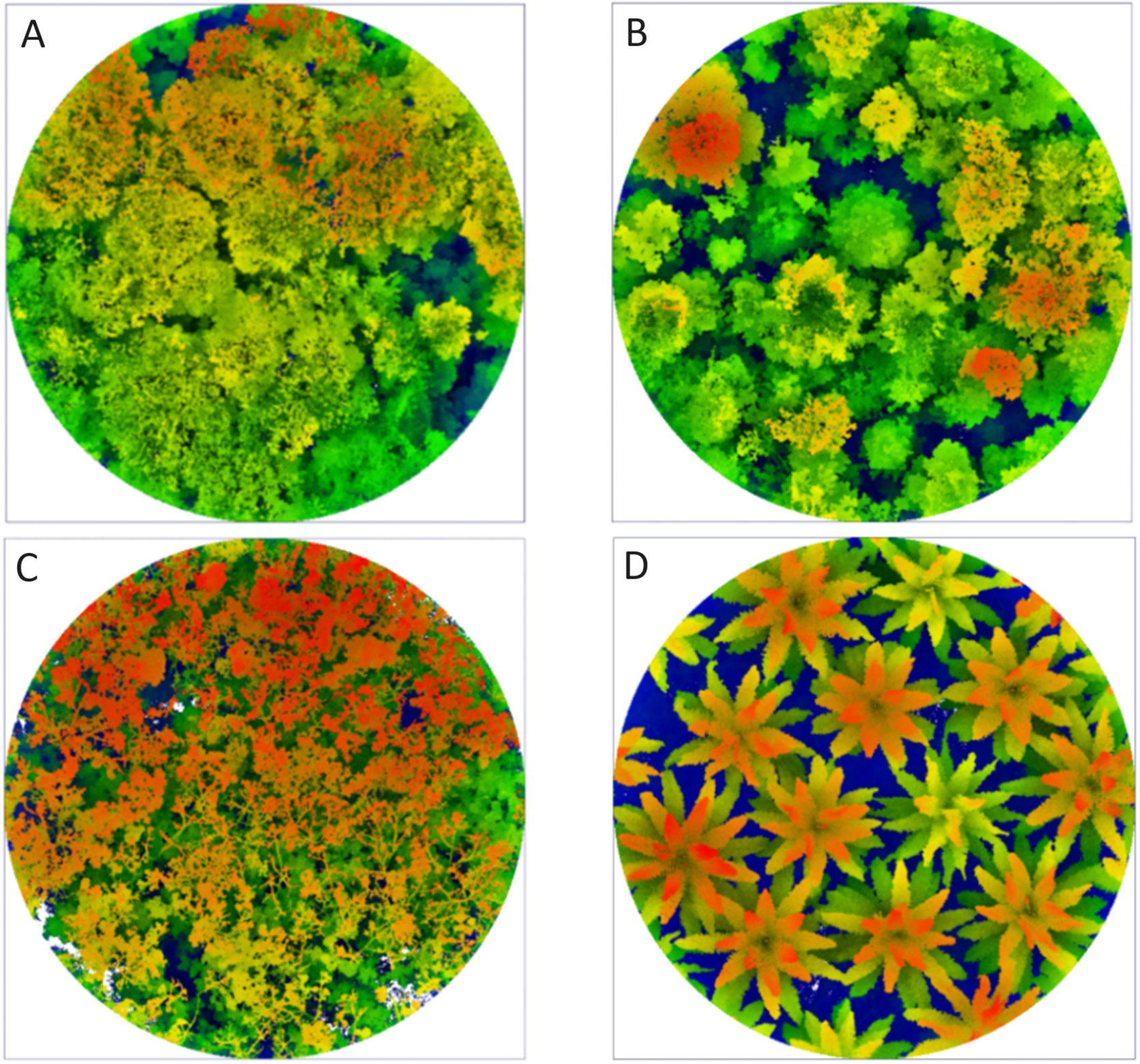
As part of the EFForTS Landscape Assessment, LiDAR data were collected from 127 plots (circular plots of 1,000 m2 size, 17.84 m radius), distributed in five clusters across the four land cover types and management regimes mentioned above over a large geographical area (Figures 1, S1, S2). This approach aimed at disentangling the influences of land cover from broader regional effects. Plot centres were located using geo-referenced points. Within each plot, three circular sub-plots, with a radius of 2.82 m each, were established, and within these, alien plants were sampled in 1 m × 1 m squares (Fig. S2). The subplots were positioned at the centre of the plot, as well as at the north and east cardinal points. Biodiversity data were only available for a subset 100 plots, and these constituted our main dataset, comprising 30 forest plots, 19 fallow land plots, 25 rubber plots, and 26 oil palm plots.
Top-down view of four LiDAR point clouds captured using a GeoSLAM ZEB Horizon LiDAR scanner, visualised with a screen-space ambient occlusion shader to distinguish between different land cover types. The colours correspond to varying heights (z-values), with each category labelled as follows: forest (A), fallow land (B), rubber (C), and oil palm (D).

Data acquisition and processing
Data for this study were collected in the Collaborative Research Centre 990 – EFForTS (https://www.uni-goettingen.de/efforts), a long-term research project with the primary objective of understanding the drivers and consequences of rainforest conversion into agricultural systems in Jambi province, Sumatra, Indonesia.
Biodiversity data
For the tree inventories, we censused all alive trees within each plot that had a diameter at breast height (dbh) ≥10 cm. Two fallow land plots did not contain any trees with diameters above the threshold and were discarded from further analyses. In the remaining plots, each tree was given a preliminary field name and for each field name in each plot, one individual was selected for the recording of field photographs and collection of an herbarium specimen for later species identification. Two duplicates were collected from sterile individuals and up to eight from flowering and/or fruiting trees. Specimens were dried and pressed and distributed to herbaria in Indonesia (BIOT, BO, herbarium of the University of Jambi) and Germany (GOET, herbarium acronyms follow Index Herbariorum: https://sweetgum.nybg.org/science/ih/). Species were identified using relevant published floras (e.g., Kiew et al. Reference Kiew, Chung, Saw, Soepadmo and Boyce2010; van Steenis et al. Reference van Steenis, de Wilde, Nooteboom, Kalkman, Kirkup, Stevens and Saw1948, van Steenis et al. Reference van Steenis, de Wilde, Nooteboom, Kalkman, Kirkup, Stevens and Saw1948; Whitmore and Ng Reference Whitmore and Ng1972). Tree diversity was calculated as the number of tree species per plot. The percentage of trees not identified to valid binomials but only to genus level (i.e., to ‘morphospecies’) was of 4.59% for forest, 3.22% for fallow land, and 0.16% for rubber plantations.
The understorey alien plant inventories focused on terrestrial vascular plant species that were not native to Sumatra. This included all herbs and ferns as well as all woody plants with a diameter at breast height < 2 cm. To estimate alien understorey diversity and biomass, all aboveground living plant mass within three 1 m × 1 m squares in subplots A, B, and C was harvested (Fig. S2) and sorted into four categories: (1) woody alien, (2) woody native, (3) herbaceous alien, and (4) herbaceous native species. The biomass of each category was stored separately, dried at 75°C for 48 hours and weighed afterwards. Alien understorey biomass was defined as the sum of alien woody and alien herbaceous biomass; native biomass was calculated accordingly. Alien plant species were identified during the sorting process and their occurrence recorded.
Tree diversity per plot was calculated for Hill numbers q = 0 (species richness), q = 1 (Hill-Shannon diversity, also referred to as effective number of species) (Chao et al. Reference Chao, Gotelli, Hsieh, Sander, Ma, Colwell and Ellison2014; Jost Reference Jost2006; Roswell et al. Reference Roswell, Dushoff and Winfree2021), using the iNEXT::iNEXT function (Hsieh et al. Reference Hsieh, Ma and Chao2016, Reference Hsieh, Ma and Chao2022) in R. We used observed, instead of rarefied/extrapolated, values because we wanted to relate the trees present within the boundaries of each plot with the vegetation structure measured within the same boundaries. We assessed sensitivity, and rarefied/extrapolated values showed similar results. Hill-Shannon diversity was selected as main metric for tree diversity throughout the study since it includes information on the relative abundances of species (Jost Reference Jost2006; Roswell et al. Reference Roswell, Dushoff and Winfree2021). Results for tree species richness are reported in the Supplementary Information.
For understorey alien plants, where no abundance data were available, we calculated the accumulated observed species richness in all three subplots per plot with the iNEXT::ChaoRichness function. The relative biomass was calculated as the fraction of alien biomass divided by the sum of alien and native biomass. Subsequent analyses used alien species richness and relative alien biomass as response variables, and Hill-Shannon diversity and species richness for tree diversity.
Mobile LiDAR data
We focused on vegetation structure metrics derived from 127 EFForTS Landscape Assessment plots, utilising mobile LiDAR scans obtained with the GeoSLAM ZEB Horizon handheld mobile laser scanner (Geoslam Ltd., Nottingham, UK). Scans were done between July 2021 and April 2022, with the scanner initiated at the centre of each circular plot and subsequently carried throughout the entire plot area of 1,000 m2. The device sends out laser beams and when reflected by any object (e.g., a trunk, branch, or leaf) records the coordinates of that object (x, y, z) relative to the plot centre, creating a point cloud of all objects.
Initial data processing was carried out using the GeoSLAM Hub software (GeoSlam Ltd., Nottingham, UK) to convert the raw scan from a .geoslam format to a .laz format that could be used for further analysis in CloudCompare software (Girardeau-Montaut Reference Girardeau-Montaut2016). In theory, the origin of the coordinate system of each scan should be the plot centre, where the scanner was initiated at the start of the scan and returned to at the end. However, deviations from this ideal case happened. Therefore, the first step in quality control using CloudCompare software was to record the x and y coordinates of the start of the scan and the distance between the start and end points. As a quality control, we established a maximum acceptable offset of 5 m; however, the maximum offset observed was lower 1 m. All scans fell in this threshold so no scans were excluded for poor quality. Still, in CloudCompare, a section of the point cloud (cross-section) was cropped for visual inspection to assess scan quality. A cleaning process was performed to remove points within 1 cm of each other (subsampling). The resulting point cloud still contained noise, which was subsequently corrected using noise filtering for points isolated by a minimum of 10 cm. The scan was then cropped to a 50 m × 50 m area centred around the centre of the plots and a vertical limit of 100 m.
Following the cleaning process in CloudCompare, LiDAR 360 software (GreenValley International, Berkeley, United States) was used. First, the scan was clipped by a circle to the dimension of the plot (1,000 m2 size). Ground points were then identified using the ‘classify ground points function’ of LiDAR360. Normalisation of the point cloud data was then performed using the ‘normalise by ground points’ function to remove the influence of terrain in the subsequent analysis. Finally, the scans were exported into two formats, .txt and .laz, for further analysis.
To select relevant metrics of vegetation structure, we first used the set of metrics introduced by Camarretta et al. (Reference Camarretta, Ehbrecht, Seidel, Wenzel, Zuhdi, Merk, Schlund, Erasmi and Knohl2021) to assess vegetation structure using airborne laser scanning data as a reference to ensure consistency with previous research in the study region. We then extended this set of metrics by considering relevant studies in the literature, including those by Atkins et al. (Reference Atkins, Bohrer, Fahey, Hardiman, Morin, Stovall, Zimmerman and Gough2018), Moudrý et al. (Reference Moudrý, Cord, Gábor, Laurin, Barták, Gdulová, Malavasi, Rocchini, Stereńczak, Prošek, Klápště and Wild2022), and Kissling and Shi (Reference Kissling and Shi2023).
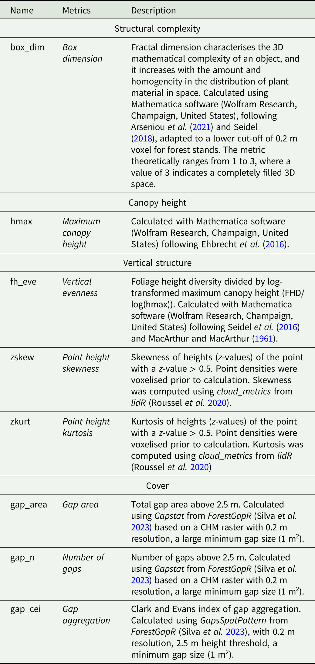
We used Mathematica (Wolfram Research, Champaign, USA) and R (R Core Team 2023) to process data and perform metric calculations. The derived selected metrics cover several aspects related to vegetation structure, including structural complexity (box dimension), height-related metrics (maximum canopy height), vertical structure (vertical evenness, foliage height evenness, point height skewness, point height kurtosis), and cover (gap area, number of gaps, gap aggregation) (Table 1, Fig. S3). Number of points were used to assess the quality of the point cloud and were excluded from all further analyses (Table S1).
List of eight LiDAR-derived metrics considered in this study. Metrics were calculated in R unless explicitly mentioned differently

Table 1. Long description
A table listing eight LiDAR-derived metrics related to vegetation structure, including structural complexity, canopy height, vertical structure, and cover. The table has three columns: Name, Metrics, and Description. The Name column lists the metric names, the Metrics column lists the corresponding metric types, and the Description column provides detailed descriptions of each metric. Row 1: Name, box_dim; Metrics, Box dimension; Description, Fractal dimension characterises the 3D mathematical complexity of an object, and it increases with the amount and homogeneity in the distribution of plant material in space. Calculated with Mathematica software (Wolfram Research, Champaign, United States) following Arseniu et al. (2021) and Seidel (2018) adapted to a lower cut-off of 0.2 m voxel for forest stands it theoretically ranges between 1 and 3, where 3 would indicate completely filled 3D space. Row 2: Name, hmax; Metrics, Maximum canopy height; Description, Calculated with Mathematica software (Wolfram Research, Champaign, United States) following Ehbrecht et al. (2016). Row 3: Name, fh_eve; Metrics, Vertical evenness; Description, Foliage height diversity divided by log-transformed maximum canopy height (FHD/log(hmax)). Calculated with Mathematica software (Wolfram Research, Champaign, United States) following Seidel et al. (2016) and MacArthur and MacArthur (1961). Row 4: Name, zskew; Metrics, Point height skewness; Description, Skewness of heights (z-values) of the point with a z-value > 0.5. Point densities were voxelised prior to calculation. Skewness was computed using cloud_metrics from lidR (Roussel et al. 2020). Row 5: Name, zkurt; Metrics, Point height kurtosis; Description, Kurtosis of heights (z-values) of the point with a z-value > 0.5. Point densities were voxelised prior to calculation. Kurtosis was computed using cloud_metrics from lidR (Roussel et al. 2020). Row 6: Name, gap_area; Metrics, Gap area; Description, Total gap area above 2.5 m. Calculated using Gapstat from ForestGapR (Silva et al. 2023) based on a CHM raster with 0.2 m resolution, a large minimum gap size (1 m^2). Row 7: Name, gap_n; Metrics, Number of gaps; Description, Number of gaps above 2.5 m. Calculated using Gapstat from ForestGapR (Silva et al. 2023) based on a CHM raster with 0.2 m resolution, a large minimum gap size (1 m^2). Row 8: Name, gap_cei; Metrics, Gap aggregation; Description, Clark and Evans index of gap aggregation. Calculated using GapsSpotPattern from ForestGapR (Silva et al. 2023), with 0.2 m resolution, 2.5 m height threshold, a minimum gap size (1 m^2).
To avoid misleading results due to the multicollinearity of variables, a correlation matrix of the initial set of variables was created, including all 20 metrics using the corrmorant::ggcorm function (Link Reference Link2020) (Fig. S4). Among variables with a high correlation (Pearson’s r ≥ 0.8), the variable considered most ecologically meaningful was chosen, the rest were excluded from further analysis.
The zq95 metric was not included from the Mobile Laser Scanning data as more points were captured at the ground level. The reduced set of variables for further analyses included eight metrics: box dimension, maximum canopy height, vertical evenness, point height skewness, point height kurtosis, gap area, number of gaps, gap aggregation (Table 1).
To examine the possible directionalities of the derived LiDAR metrics, a PCA was undertaken using the FactoMineR::PCA function (Lê et al. Reference Lê, Josse and Husson2008) in R (Fig. S5). The PCA was visualised as a biplot with the function factoextra::fviz_pca_biplot (Kassambara and Mundt Reference Kassambara and Mundt2020). Since gap aggregation cannot be calculated when <2 gaps are present, we imputed the value of gap aggregation for 34 plots as the mean of the land cover of the respective plot. The resulting dataset of structure variables was used for all further analysis.
Statistical analysis
Data distributions were inspected using the inspectdf::inspect_num and inspectdf::show_plot functions (Rushworth Reference Rushworth2022). Log transformations (log10) were applied to variables with highly skewed distributions, for zkurt as log10 (zkurt + 0.01) and gap_area as log10 (gap_area + 1).
Model of the relationship diversity structure
First, we examined the relationship between tree diversity (q = 1 and q = 0) and vegetation structure. We initially evaluated simple linear models for all structural metrics. To account for the cluster plot design, we compared these against linear mixed-effects models with ‘site’ as random effect using Akaike Information Criterion (AIC). For most of the metrics, the simpler model was sufficient. However, for maximum canopy height, number of gaps, and alien species richness, the mixed-effects models provided a better fit. Across all models, land cover and the respective tree diversity metric were included as fixed effect to predict structural metrics (e.g., formula: gap_n ∼ q1 + land cover + (1 | site)).
To assess the relationship between vegetation structure and both the species richness and relative biomass of alien understorey plants, we fitted generalised linear mixed models (GLMMs) using the glmmTMB package. We modelled species richness using a Conway-Maxwell Poisson distribution and relative biomass using an ordered beta distribution. For each model, a specific structural variable and land cover were included as fixed effects, with ‘site’ as random effect (e.g., formula = q0_alien ∼ box_dim + land cover + (1|site) (Brooks et al. Reference Brooks, Kristensen, Benthem, van, Berg, Nielsen, Skaug, Mächler and Bolker2017). To determine whether the relationship between alien species richness and relative biomass with the predictor variables was explicitly non-linear, we compared the AIC of GLMs fitted with linear terms against quadratic terms (Table S10, Table S11). In the alien species richness individual model, a quadratic term was added for maximum canopy height, point height skewness, gap area, and gap aggregation. In the relative biomass individual model, a quadratic term was added for box dimension, point height skewness, gap area and gap aggregation. Model fit of all the models was first assessed using performance::check_model function (Lüdecke et al. Reference Lüdecke, Ben-Shachar, Patil, Waggoner and Makowski2021). Additionally, overdispersion and zero inflation were also assessed using performance::check_overdispersion and performance::check_zeroinflation.
We fitted two global generalised linear models, to identify the most robust predictors of alien species richness and relative biomass. Both global models included the exact same suite of predictors: box dimension, maximum canopy height, vertical evenness, point height skewness, gap area, number of gaps, gap aggregation, Hill-Shannon diversity, and land cover. We used a Conway-Maxwell-Poisson distribution to model species richness and an ordered beta distribution for relative biomass. All predictors were centred and standardised to make all the model coefficients comparable using the scale function. We assessed model fit and multicollinearity using the function performance::check_model (Lüdecke et al. Reference Lüdecke, Ben-Shachar, Patil, Waggoner and Makowski2021). We then used a model selection process to identify the most robust predictors using MuMIn::dredge (Bartoń Reference Bartoń2024), which tests all models nested in the global model, i.e., all possible combinations of predictor variables. The set of models was defined based on the criterion of a deltaAICc lower than 2, and the models were ranked based on their AICc, using MuMIn:: get.models (Bartoń Reference Bartoń2024). To avoid defining the best model, we used model averaging using MuMIn::model.avg. Additionally, the weight or also called the relative importance value for each predictor variable in the model was analysed using MuMIn::sw (Bartoń Reference Bartoń2024). Model assumptions were reassessed using performance::check_model (Lüdecke et al. Reference Lüdecke, Ben-Shachar, Patil, Waggoner and Makowski2021). Finally, we examined the spatial autocorrelation in the model’s residuals (Moran’s I) using the DHARMa::testSpatialAutocorrelation, we found no spatial autocorrelation (Table S5) (Hartig Reference Hartig2022).
All statistical analyses were performed using version 4.4.1 of the R statistical software (R Core Team 2023). Initial data exploration was conducted using inspectdf (v0.0.12; Rushworth Reference Rushworth2022). Data directionalities using FactoMineR::PCA function (v2.11; Lê et al. Reference Lê, Josse and Husson2008) and factoextra:: fviz_pca_biplot (v1.0.7; Kassambara and Mundt Reference Kassambara and Mundt2020). Correlation matrix using corrmorant::ggcorm (v0.0.0.9007; Link Reference Link2020). Diversity estimates were generated using iNEXT (v3.0.1; Hsieh et al. Reference Hsieh, Ma and Chao2022). GLMs were implemented via glmmTMB (v1.1.10; Brooks et al. Reference Brooks, Kristensen, Benthem, van, Berg, Nielsen, Skaug, Mächler and Bolker2017) and linear mixed model with lme4 (v1.1-35.5; Bates et al. Reference Bates, Mächler, Bolker and Walker2015). Model fit and diagnostic checks were conducted using DHARMa (v0.4.6; Hartig Reference Hartig2022) and the performance package (v0.10.8; Lüdecke et al. Reference Lüdecke, Ben-Shachar, Patil, Waggoner and Makowski2021). Model selection were performed using MuMIn (v1.48.4; Bartoń Reference Bartoń2024).
Results
Land cover shapes vegetation structure
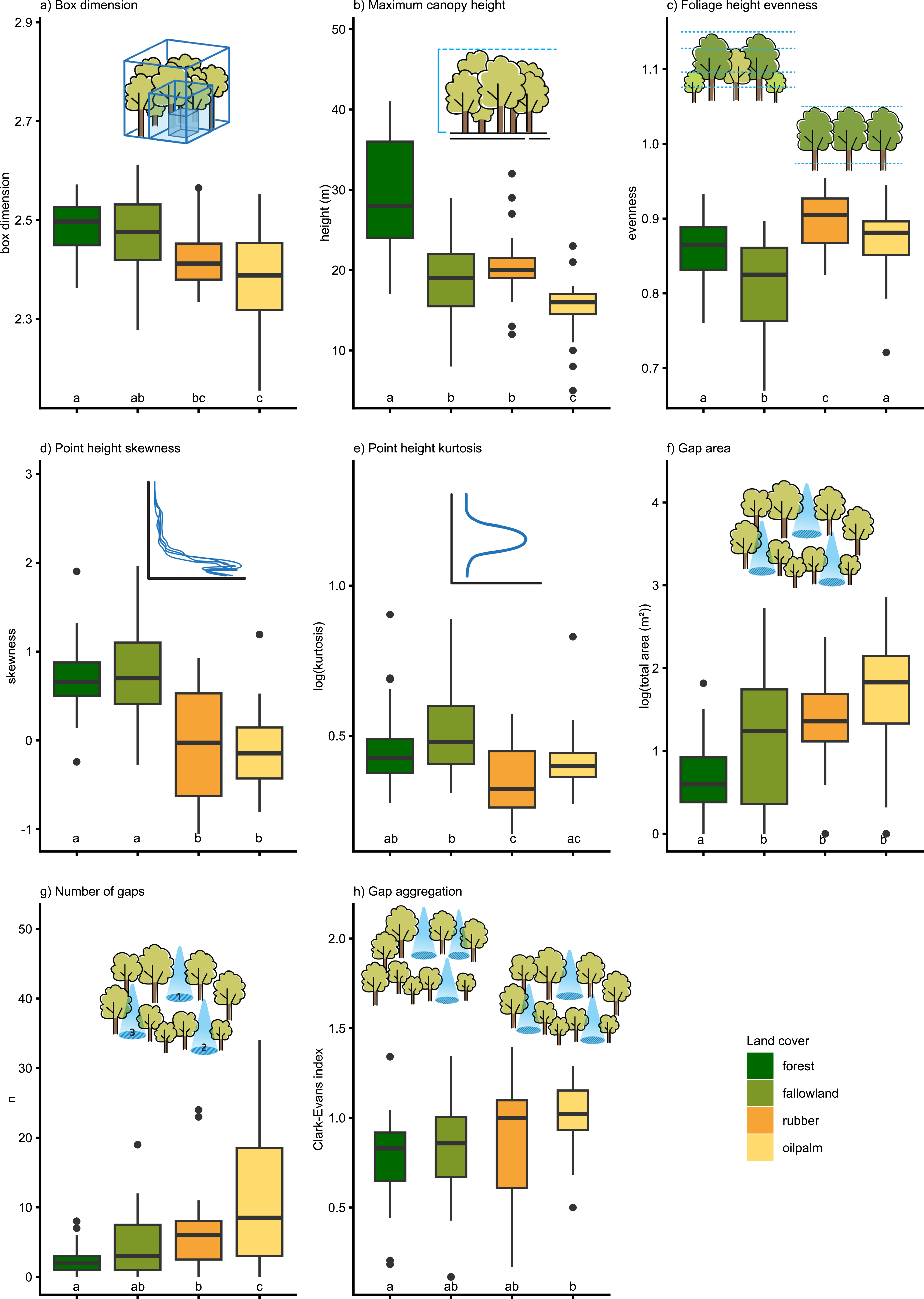
All vegetation structure variables showed significant differences between the analysed land cover types. However, patterns differed depending on the variables. Box dimension and maximum canopy height decreased with increasing land cover intensity, i.e., from forest (mean box dimension = 2.49, mean maximum canopy height = 29.09 m) over fallow land and rubber to oil palm (mean box dimension = 2.38, mean maximum canopy height = 15.03 m) while gap area and the number of gaps increased in the same direction (forest: mean gap area = 0.65 m2, mean number of gaps = 2.09; oil palm: mean gap area = 1.69 m2, mean number of gaps = 12.5). Gap aggregation showed higher values in oil palm (mean = 1.01), indicating a distribution more towards uniform compared to the other land cover types.
Variables describing the vertical vegetation structure showed different patterns: in fallow land, vertical evenness was significantly lower (mean = 0.81) than in the other land cover types, indicating that in fallow land the vegetation clustered more at one particular height. Point height skewness was significantly higher in forests (mean = 0.69) and fallow land (mean = 0.79), indicating a denser understorey there. Point height kurtosis showed similar patterns (forest: mean = 0.46, fallow land: mean = 0.52) (Figure 2).
Variation of eight structural metrics across the four land cover types studied: forest, fallow land, rubber, oil palm. Statistically significant differences among land cover types (p < 0.05) are denoted by letters. A non-parametric Kruskal–Wallis test, followed by post hoc Dunn tests for pairwise comparisons, was conducted for gap aggregation (h) and point height kurtosis (e). For the remaining metrics, a Welch-ANOVA and Games-Howell post hoc test were applied.

High tree diversity is linked with high structural complexity
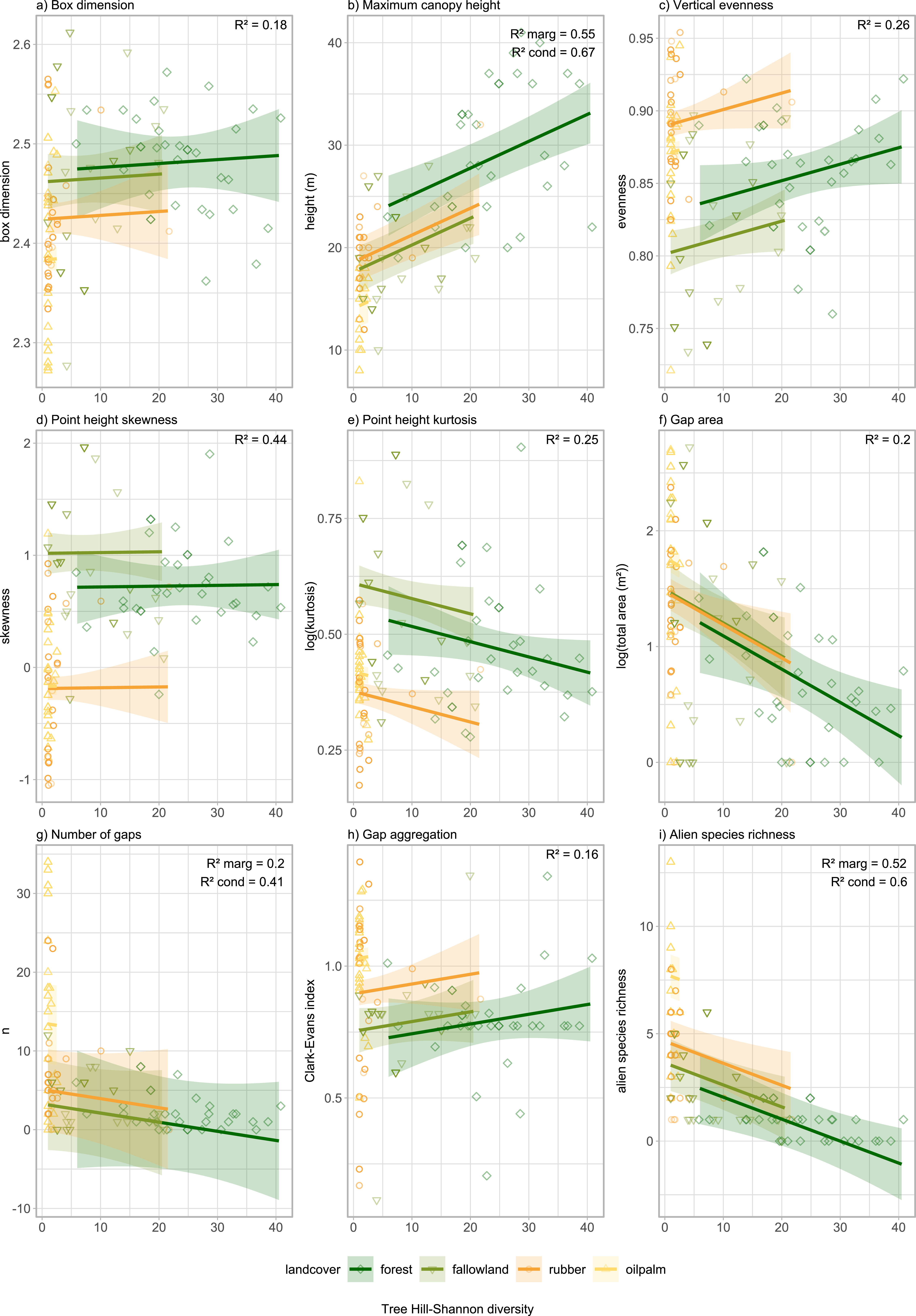
Tree diversity, alongside land cover, was a strong driver of structural metrics. Forest exhibited greater variability across all metrics compared to oil palm. Tree Hill-Shannon diversity was positively correlated with maximum canopy height (R 2 marg = 0.55) and negatively correlated with gap area (R 2 = 0.2) and alien species richness (R 2 marg = 0.52). This suggests that diverse tree communities result in taller trees, smaller gap areas, and lower alien species richness (see Figure 3, Table S4).
Relationships between Hill-Shannon diversity (q = 1) of trees and eight vegetation structure variables in four land cover types of Jambi Province, Sumatra, Indonesia. Results of simple linear models, except for number of gaps, alien understorey plant species richness, and maximum canopy height, for which linear mixed model with site as random effect was used. Each land cover types are shown as simple lines with 95% confidence intervals. Each point represents one of 100 plots.

Similar trends were observed for tree species richness, which was positively correlated with structural variables, such as maximum canopy height and vertical evenness (R 2 = 0.27), but negatively associated with alien species richness (R 2 marg = 0.52), gap aggregation (R 2 = 0. 17), gap area (R 2 = 0.21), point height kurtosis (R 2 = 0.26) (Fig. S6, Table S3).
Vegetation structure is associated with alien plants
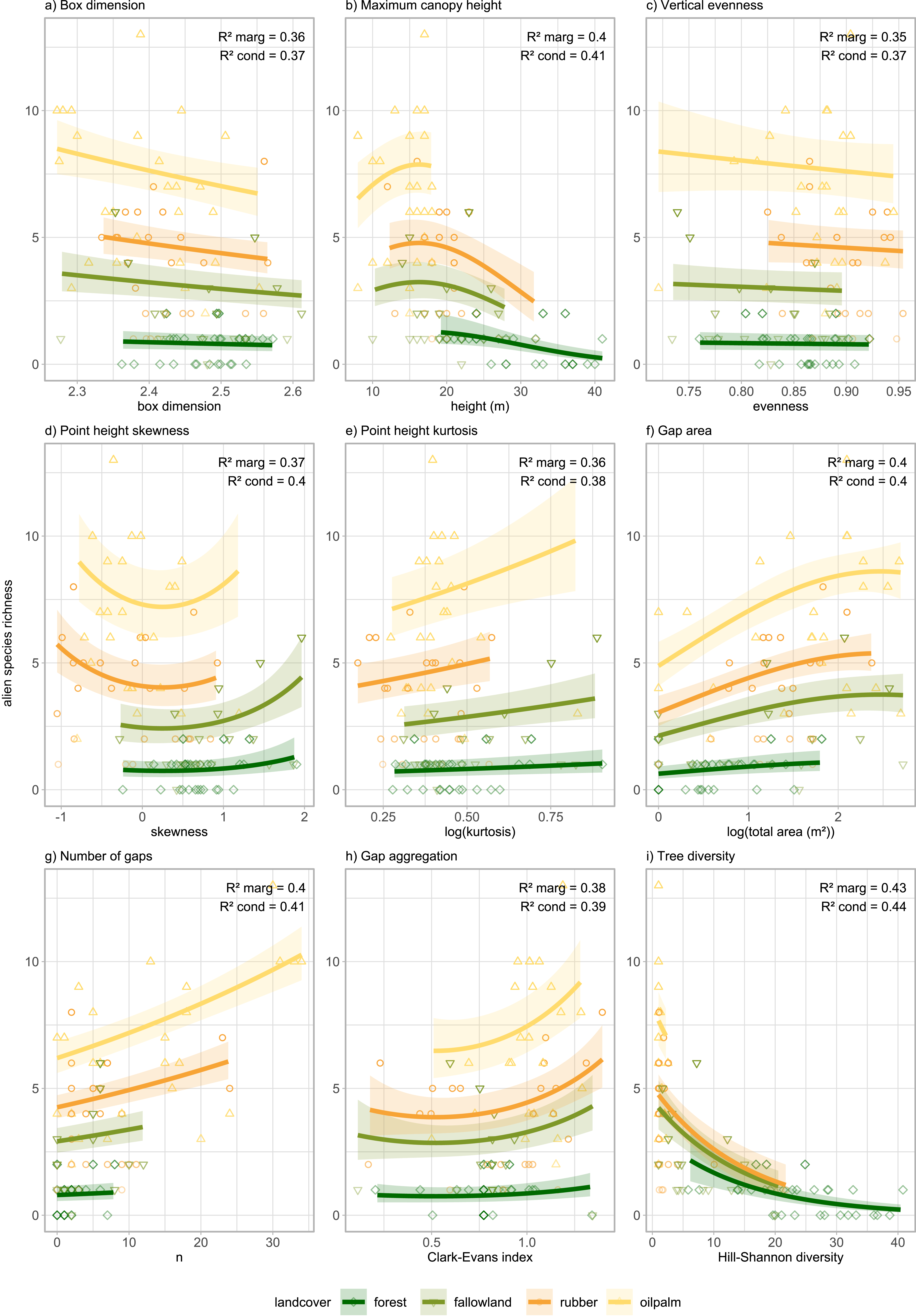
Alien plant diversity was higher in more intensively managed systems (Fig. S12). Land cover had a strong effect on species richness and relative biomass of alien species. Most metrics were significant drivers of both outcomes (e.g., maximum canopy height, tree Hill-Shannon diversity, number of gaps). However, vertical evenness and the linear effect of gap aggregation were drivers of alien relative biomass only (Fig. S7, Table S5). Furthermore, the linear effect of gap area was only significant for alien species richness (Figure 4, Table S6).
Relationship between alien understorey plant species richness and eight vegetation structure variables in four land cover types of Jambi Province, Sumatra, Indonesia. Results of generalised linear mixed models with site as random effect. Each line represents a land cover type with 95% confidence intervals. A quadratic term was added for maximum canopy height, point height skewness, gap area, and gap aggregation. Each point represents one of 100 plots.

Vegetation structure and tree diversity drive alien plant invasion
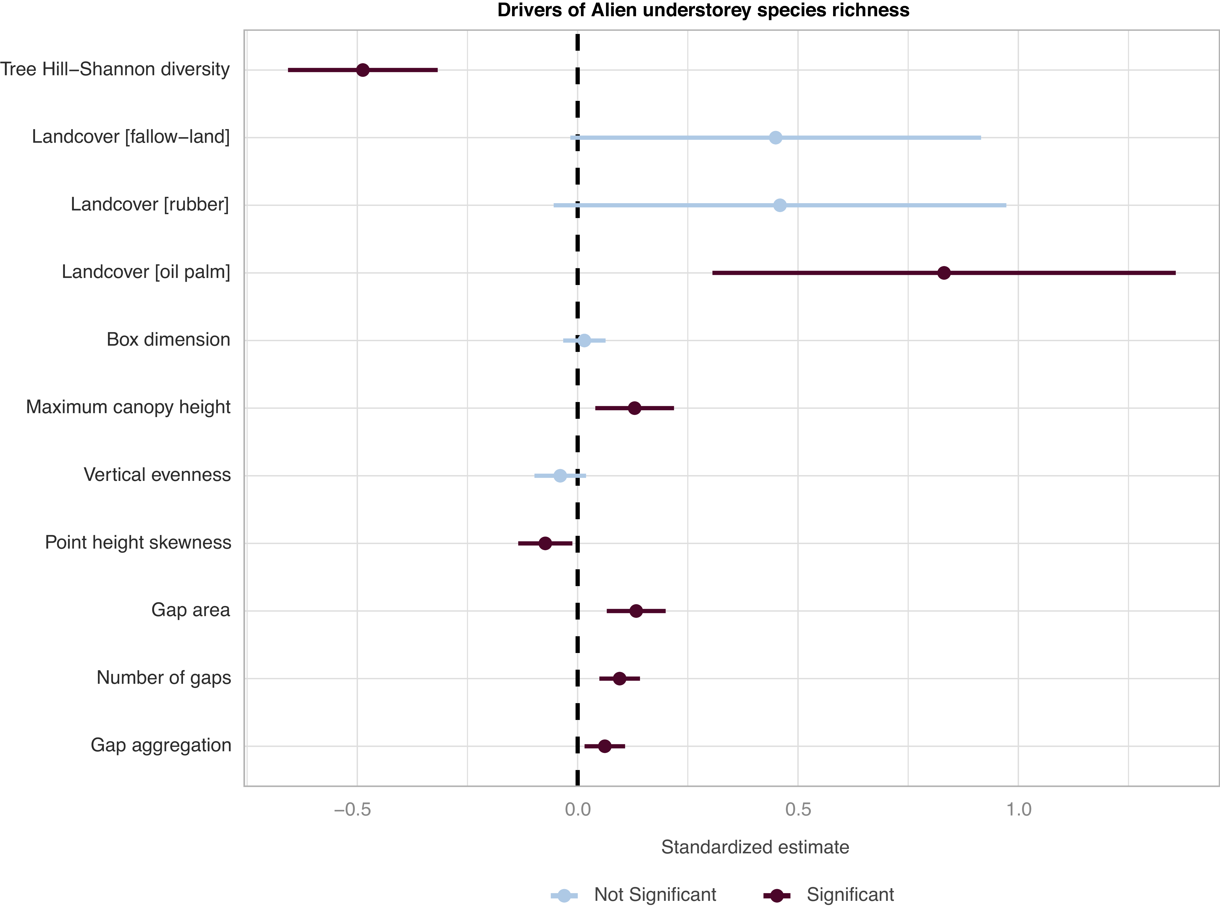
Land cover is a strong driver of alien species presence, with the effect being more pronounced in oil palm habitats. Alien presence was positively correlated with structural metrics indicative of open and disturbed areas such as gap metrics and height. Furthermore, tree Hill-Shannon diversity and vertical evenness negatively affected alien species (Figure 5). Alien presence and abundance are highest in environments with open canopies and few understorey (Figure 5, S8).
Standardised model coefficients for multiple regression of alien understorey plant species richness against predictors of vegetation structure, Tree Hill-Shannon diversity and land cover. Result of model averaging of a generalised linear model following a Conway–Maxwell–Poisson distribution. All predictors were standardised.

Discussion
This study examined 100 plots across a human-modified tropical landscape to investigate how vegetation structure and tree diversity influence plant invasibility. Our results reveal that tropical land cover change alter almost all aspects of vegetation structure (see Figure 2). Land-use intensification results in shorter vegetation, reduced vertical complexity, and an increase in the number and size of canopy gaps. Tree diversity was positively associated with metrics reflecting canopy height, as well as point height kurtosis and vertical evenness, both of which are indicators of dense and layered vegetation. In contrast, alien plant diversity was higher in more open, structurally simpler vegetation. However, there is some limitation in our dataset: the small sampling area of alien plants (3 m2) may not fully capture their patchy distribution in some plots.
Tree diversity and vegetation structure as drivers of invasibility
Our results show that tree diversity is linked to lower invasibility, an association that appears mediated by vegetation structure. There was a positive association between tree diversity (species richness and Hill-Shannon diversity) and maximum canopy height and negatively associated with gap area and alien species richness (Figures 3 and 5, Table S4). This suggests that diverse tree communities tend to have denser, taller canopies with fewer gaps, creating more complex vertical and horizontal structures. Closed canopies reduce light availability, creating conditions that limit the establishment of light-demanding alien species, particularly those that are shade intolerant (Denslow and DeWalt Reference Denslow, DeWalt, Carson and Schnitzer2008; Waddell et al. Reference Waddell, Banin, Fleiss, Hill, Hughes, Jelling, Yeong, Ola, Sailim, Tangah and Chapman2020a).
High tree diversity supports a wider range of functional traits and crown architectures. Different crown shapes, leaf arrangements, and light-use strategies enable species to occupy distinct layers, resulting in effective niche partitioning. In this context, the box dimension metric can be interpreted as a proxy for canopy space occupation. The strong relationship between Hill-Shannon diversity of trees and maximum canopy height (R 2 marg = 0.55) suggests that more diverse tree communities exhibit denser, more structurally complex canopies (Figure 3). These structurally complex canopies in combination with a dense understorey vegetation restrict light penetration to the forest floor, leaving little to no opportunity for alien plants to establish (Martin et al. Reference Martin, Canham and Marks2009).
These results support the biological resistance hypothesis, which suggests that tropical forests are naturally resistant to invasions due to their high native density (Elton Reference Elton and Elton1958). This resistance is driven by reduced resource availability and strong competition from native species for space, light, and nutrients (MacArthur Reference MacArthur1965; Mungi et al. Reference Mungi, Galetti, Ratnam, Chala, Sanín and Svenning2025).
Human-mediated disturbance weakens resistance to alien plant invasion
Human land management, particularly the conversion of forests to plantations, alters ecosystem structure and dynamics. We found that land-use intensification led to a strong decline in tree diversity (see Fig. S13), a result supported by other studies (Marsh et al. Reference Marsh, Turner, Blonder, Bongalov, Both, Cruz, Elias, Hemprich-Bennett, Jotan, Kemp, Kritzler, Milne, Milodowski, Mitchell, Pillco, Nunes, Riutta, Robinson, Slade, Bernard, Burslem, Chung, Clare, Coomes, Davies, Edwards, Johnson, Kratina, Malhi, Majalap, Nilus, Ostle, Rossiter, Struebig, Tobias, Williams, Ewers, Lewis, Reynolds, Teh and Hector2025; Rembold et al. Reference Rembold, Mangopo, Tjitrosoedirdjo and Kreft2017). In addition, land-use intensification is also accompanied by a decline in structural complexity. Higher abundance and diversity of alien plants (Fig. S12) were present in plantations characterised by open vegetation with a large number of gaps and low canopies vegetation, whereas forests were almost devoid of alien plants (Figures 2, S12, Table S10). Here, gap metrics (e.g., number of gaps, gap aggregation and gap area) can be interpreted as proxies for light availability. In this regard, open plantations generally offer favourable conditions for the establishment of alien plants (Pyšek et al. Reference Pyšek, Hulme, Simberloff, Bacher, Blackburn, Carlton, Dawson, Essl, Foxcroft, Genovesi, Jeschke, Kühn, Liebhold, Mandrak, Meyerson, Pauchard, Pergl, Roy, Seebens, van Kleunen, Vilà, Wingfield and Richardson2020; Wang et al. Reference Wang, Fang, Sanders, White and Tang2009). This highlights the preference of alien plants for more open and disturbed habitats (Figures 4 and 5) (Fine Reference Fine2002; Rembold et al. Reference Rembold, Mangopo, Tjitrosoedirdjo and Kreft2017). Open canopies create hotter and drier microclimates (Pallavi et al. Reference Pallavi, Marques, Ramadhani, Valdes-Uribe, Hendrayanto and Hölscher2024), influencing the distribution of alien plants (Davis et al. Reference Davis, Dobrowski, Holden, Higuera and Abatzoglou2019; Drescher et al. Reference Drescher, Rembold, Allen, Beckschäfer, Buchori, Clough, Faust, Fauzi, Gunawan, Hertel, Irawan, Jaya, Klarner, Kleinn, Knohl, Kotowska, Krashevska, Krishna, Leuschner, Lorenz, Meijide, Melati, Nomura, Pérez-Cruzado, Qaim, Siregar, Steinebach, Tjoa, Tscharntke, Wick, Wiegand, Kreft and Scheu2016; Rembold et al. Reference Rembold, Mangopo, Tjitrosoedirdjo and Kreft2017).
Common management practices in plantations include fertilisation, liming, weeding, and pesticide application, and these may significantly impact the establishment and spread of alien species. Weeding leads to increased resource availability, a well-established driver of invasions (Martin et al. Reference Martin, Canham and Marks2009). Likewise, the management of understorey vegetation through application of herbicides or manual weeding may create conditions that favour the proliferation of alien species, as they tend to regenerate faster or thrive better in disturbed conditions than native species (Iddris et al. Reference Iddris, Formaglio, Paul, von Groß, Chen, Angulo-Rubiano, Berkelmann, Brambach, Darras, Krashevska, Potapov, Wenzel, Irawan, Damris, Daniel, Grass, Kreft, Scheu, Tscharntke, Tjoa, Veldkamp and Corre2023; Pyšek et al. Reference Pyšek, Hulme, Simberloff, Bacher, Blackburn, Carlton, Dawson, Essl, Foxcroft, Genovesi, Jeschke, Kühn, Liebhold, Mandrak, Meyerson, Pauchard, Pergl, Roy, Seebens, van Kleunen, Vilà, Wingfield and Richardson2020; Rembold et al. Reference Rembold, Mangopo, Tjitrosoedirdjo and Kreft2017).
While vegetation structure, diversity, and disturbance are key factors explaining invasibility, other drivers can also play a role. Propagule pressure, though not directly measured in this study, is a well-known contributor to plant invasions, particularly in human-disturbed environments where it is elevated. For example, juveniles of rubber (Hevea brasiliensis) and oil palm (Elaeis guineensis) predominantly occurred in rubber and oil palm plantations, respectively, suggesting that propagule pressure from nearby planted trees is an important factor for their establishment (Table S10). In addition, alien species differ in their invasiveness, a result of specific traits (Elton Reference Elton and Elton1958; Waddell et al. Reference Waddell, Chapman, Hill, Hughes, Bin Sailim, Tangah and Banin2020b). In our study, no herbaceous alien plants were able to establish in forests, although they were often abundant in fallow land and plantations (Fig. S12, Table S10). Overall, the alien communities were heavily dominated by a few well-known invasive species, like Asystasia intrusa (Acanthaceae), Miconia crenata (Melastomataceae), Spermacoce alata (Rubiaceae) and various grasses (Poaceae; see Table S10 for a full list of species). Possibly, these species have overcome native resistance due to superior colonisation abilities or benefited from enemy release (Keane and Crawley Reference Keane and Crawley2002). The majority of the alien species were found in oil palm and sometimes also in rubber, attesting to their adaptation to disturbed environments (Kiew and Vollesen Reference Kiew and Vollesen1997; Waddell et al. Reference Waddell, Chapman, Hill, Hughes, Bin Sailim, Tangah and Banin2020b). Notably, the two Melastomataceae species Miconia crenata and Bellucia pentamera stood out in being able to invade forest areas. Both are known as aggressive invasives and should be monitored closely (DeWalt et al. Reference DeWalt, Denslow, Johnson, Goldenberg, Michelangeli and Almeda2022; Padmanaba et al. Reference Padmanaba, Tomlinson, Hughes and Corlett2017; Rejmánek and Richardson Reference Rejmánek and Richardson2013; Solfiyeni et al. Reference Solfiyeni, Chairul and Mukhtar2022). The inherent resistance of intact forests is not absolute as some alien plants are able to establish under closed canopy.
Implications
Our results provide evidence that, under low disturbance, native diversity and structurally complex environments naturally limit invasibility. However, land cover change and intensive management disrupt these natural barriers. To mitigate alien plant invasions, our findings highlight the importance of maintaining or restoring complex vegetation structure, specifically by minimising the creation of large canopy gaps. This could create more resilient and ecologically stable ecosystems (sensu Seidel and Ammer Reference Seidel and Ammer2023). Effective forest management should then incorporate both biodiversity conservation goals with efforts to preserve or restore structural complexity, especially in landscapes experiencing rapid land cover changes (Paterno et al. Reference Paterno, Brambach, Guerrero-Ramírez, Zemp, Cantillo, Camarretta, Moura, Gailing, Ballauff, Polle, Schlund, Erasmi, Iddris, Khokthong, Sundawati, Irawan, Hölscher and Kreft2024; Zemp et al. Reference Zemp, Guerrero-Ramirez, Brambach, Darras, Grass, Potapov, Röll, Arimond, Ballauff, Behling, Berkelmann, Biagioni, Buchori, Craven, Daniel, Gailing, Ellsäßer, Fardiansah, Hennings, Irawan, Khokthong, Krashevska, Krause, Kückes, Li, Lorenz, Maraun, Merk, Moura, Mulyani, Paterno, Pebrianti, Polle, Prameswari, Sachsenmaier, Scheu, Schneider, Setiajiati, Setyaningsih, Sundawati, Tscharntke, Wollni, Hölscher and Kreft2023).
Supplementary material
The supplementary material for this article can be found at https://doi.org/10.1017/S0266467426100777.
Data availability statement
The data used for this study are available on the GRO.data repository:
Brambach F, Kabache S, Tjitrosoedirdjo SS and Kreft H (2023a, September 17) EFForTS Landscape Assessment (LA) - B06 mobile LiDAR metrics. GRO.data. https://doi.org/10.25625/P77SA6.
Brambach F, Kotowska M, C. M. Moura, Kabache S, Tjitrosoedirdjo SS and Kreft H (2023b) EFForTS Landscape Assessment (LA) - B06 tree diversity. GRO.data. https://doi.org/10.25625/9GSSSA.
Brambach F, Kotowska M, C. M. Moura, Tjitrosoedirdjo SS and Kreft H (2023c) EFForTS Landscape Assessment - B06 Understorey alien plant species. GRO.data. https://doi.org/10.25625/HZRGZV.
Camarretta N, Knohl A, Erasmi S and Schlund M (2021) Landscape Assessment (LA) centre plot coordinates. Göttingen Research Online / Data. https://doi.org/10.25625/SSN6RO.
Acknowledgements
We are indebted to our study regions’ farmers, P.T. REKI, P.T. Humusindo, P.T. Perkebunan Nusantara VI, and the Bukit Duabelas National Park authorities for their support and cooperation, granting us access to the research sites and providing valuable information. We also thank our dedicated staff at the EFForTS offices in Jambi, Bogor, and Göttingen for their exceptional coordination. Special thanks are extended to our field teams, whose hard, independent work was essential to the successful completion of this research. Ira Taliki (SatuNol Studio, Palu, Indonesia) designed icons and figures, which we gratefully acknowledge. We thank BRIN (National Research and Innovation Agency, Indonesia) for granting research permits (46/E5/E5.4/SIP.EXT/2019 and 232/SIP/IV/FR/10/2022).
Author contribution
Conceptualisation: FB, HK. Data curation: SK, FB, DS. Formal analysis: SK. Funding acquisition: HK, FB, DS. Investigation: FB, HK, AT. Methodology: SK, FB, DS, HK, KP. Project administration: AT, FB. Resources: AT, SST. Software: SK. Supervision: AT, SST, FB. Visualisation: SK. Writing – original draft: SK, FB. Writing – review & editing: all authors.
Financial support
This study was funded by the Deutsche Forschungsgemeinschaft (DFG, project number 192626868) as part of the collaborative German-Indonesian research project CRC990 – EFForTS, subproject B06. Sarah Kabache was further supported by a fellowship of 44moles GmbH, Göttingen, Germany. We thank both funders for their support of this research.
Competing interests
The authors declare no conflict of interest.


 Open access

