II. EXPERIMENTAL METHODS

An Al–4 wt% Mg–0.3 wt% Sc alloy was homogenized at 848 K for 6 h and then aged at 553 K for 8 h to produce Al₃Sc precipitates. Specimens for TEM observation were prepared using twin-jet electropolishing in a 33% nitric acid/67% methanol solution at 245 K and 6 V.

Acquisition of tilt-series images and additional microstructural analyses were carried out using a 2010(LaB₆) transmission electron microscope (TEM; JEOL, Tokyo, Japan) operating at 200 kV using a standard double-tilt holder with a tilt range of ∼±35°. The dataset was collected by aligning one Kikuchi band with the primary axis of tilt, which was enabled near maximum angular collection. The imaging method used, unless otherwise indicated, was weak-beam dark-field imaging with the same g-vector and deviation parameter maintained over the entire tilt-series—the diffraction vectors were of low order and a (g, 3g) condition was used. Micrographs were recorded with a Smartscan CCD camera (Gatan, Pleasanton, CA) in gain-normalized mode.

Images from the tilt-series were aligned using the EM3D 2.0 software with a number of computer-assigned and user-defined markers, most of which corresponded to small defects a few nanometer in size or dislocation junctions, as these features were easy to identify and remained present throughout the series. Construction of a 3D visualization model was enabled by tracing and labeling the dislocations using toolsets within University of California, San Francisco Chimera software (build 1.4.1).

III. RESULTS AND DISCUSSION

Before presenting the results from the tomographic reconstruction of dislocation reactions, a method for incorporating the specimen coordinate system within the tomogram was developed. This capability is essential for a complete analysis of the dislocation interactions in, for example, the determination of the slip plane on which dislocation lines and loops reside. The method utilizes matching projected distances and the angles between these projected vectors in the tomogram and in an electron micrograph acquired at a known beam direction, preferably at a major zone. When a match is found, the relationship between the reciprocal and real lattice vectors is used to assign directions in the tomogram. This process is repeated for several different beam directions. Using this approach, it is possible to position a correctly oriented Thompson tetrahedron in the tomogram and the 3D model that rotates with both.

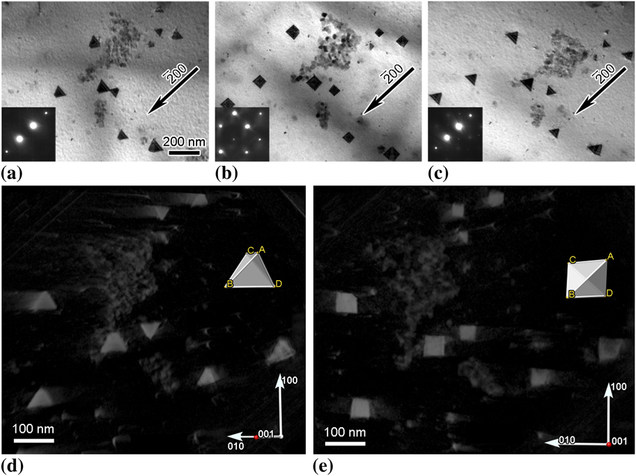
To illustrate the viability of the approach and to estimate its accuracy, a tomogram of large stacking-fault tetrahedra in quenched gold was reconstructed from a series of images acquired over the angular range from −29.1° to +39.3°; this corresponded to traversing from the zone through the (001) zone, to just pass (012). The tetrahedra are bound by stair-rod dislocations that lie along the <110> edges of the {111} planes that form the tetrahedra. For the same diffraction vector, the projected shape of a tetrahedron depends on the beam direction and changes from triangular form near a {110} type zone to square at {001} zone, then back to triangular form as the beam direction approaches another {110} zone. These changes in projected image shape are seen in the bright-field micrographs presented in Figs. 1(a)–1(c). Knowing that the edges of the tetrahedron must lie along <110> directions provides an internal reference that can be used to verify the placement of lattice directions and a Thompson tetrahedron locked within the tomogram. Using this approach for multiple beam directions, it was found that the Thompson tetrahedron could be oriented within ±3° of the projected edges of the actual tetrahedra. The correlation between the Thompson tetrahedron and the Au tetrahedra can be ascertained from the snapshots from different viewing directions presented in Figs. 1(d) and 1(e) and in supplemental movie file 1.

FIG. 1.

(a)–(c) Change in the projected image of stacking fault tetrahedra in Au for the same diffraction vector but different beam directions. Beam directions were near [011], [001], and []for images (a), (b), and (c), respectively. (d) and (e) Select snapshots of the tomographic reconstruction of the tetrahedra showing the projected shape along with a Thompson tetrahedron inserted based on a constellation matching method. The [001] direction, marked with a red dot on the coordinate axes, is coming out of the page at (d) ∼45° and (e) ∼90°.

From previousReference Clark, Robertson, Dougherty, Ahn and Sofronis² and current post-deformation and time-resolved TEM straining experiments on particle-strengthened alloys, it is known that there is a wide variety of possible interactions between dislocations and particles. These interactions generate dislocation structures on and adjacent to the particles. The electron micrographs presented in Fig. 2 show examples of possible structures generated by dislocation–particle interactions. In these images, dislocation lines and loops can be seen extending from the particles and existing separate from them. Some line dislocations extend between the particles, suggesting that they were produced by an interaction that involved multiple particles [Figs. 2(c) and 2(d)]. This formation mechanism has been observed in time-resolved in situ TEM straining experiments. Similarly, the loops away from the particle are generated as part of the dislocation–particle interaction, with the loop pinching off and breaking free after completion of the interaction. Although the time-resolved experiments provided insight about the sequence and dynamics of dislocation–particle interactions, discovering the reasons for the different interactions is limited as information on the spatial relationship is missing. The dislocation dynamic simulations demonstrated that knowledge of this spatial relationship was important to differentiate between the various reaction possibilities.Reference Xiang, Srolovitz, Cheng and Weinan^4, Reference Xiang, Chang, Srolovitz and Weinan⁵

FIG. 2.

Examples of dislocation structures created through the interaction of dislocations with Al₃Sc particles in an Al–Mg–Sc alloy.

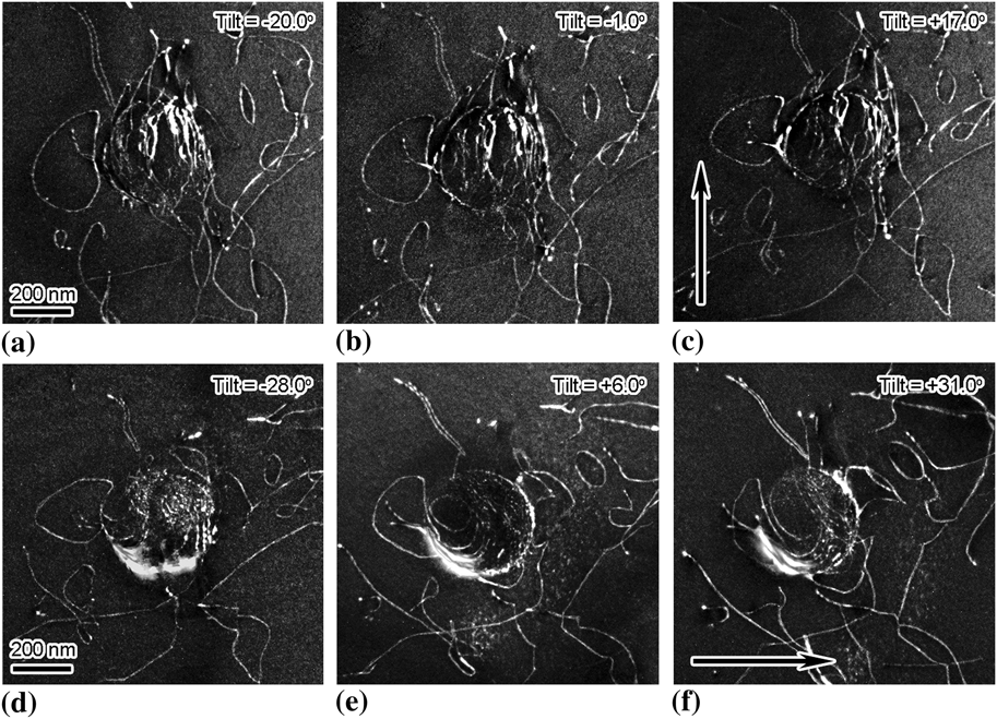
To explore the feasibility of using tomograms to provide information on the spatial relationship between the dislocations and the particles, weak-beam dark-field images of such interactions in lightly deformed samples of an Al–Mg–Sc alloy were acquired every one degree over an angular range of −28° to +32° (X-tilt only) while maintaining a constant deviation parameter and diffraction vector. In one case, two image sets were acquired with orthogonal 020-type diffraction vectors with the intent of combining them to reduce the missing wedge effect—this proved impractical for this image set because of intensity variations and the loss of visibility of some dislocations as they satisfied the |g·b| invisibility condition. Select images from both sets are presented in Figs. 3(a)–3(c) for one diffraction vector, g = and Figs. 3(d)–3(f) for the other, g = 200. Dislocations are seen curved around the particle, partial loops are attached to the particle interface, and dislocation loops and lines extend away from the particle. Application of g·b analysis revealed that the majority of the dislocations have a common Burgers vector of —these have been colored differently from each other for clarity of visualization. The rest of the dislocations, traced in white in Figs. 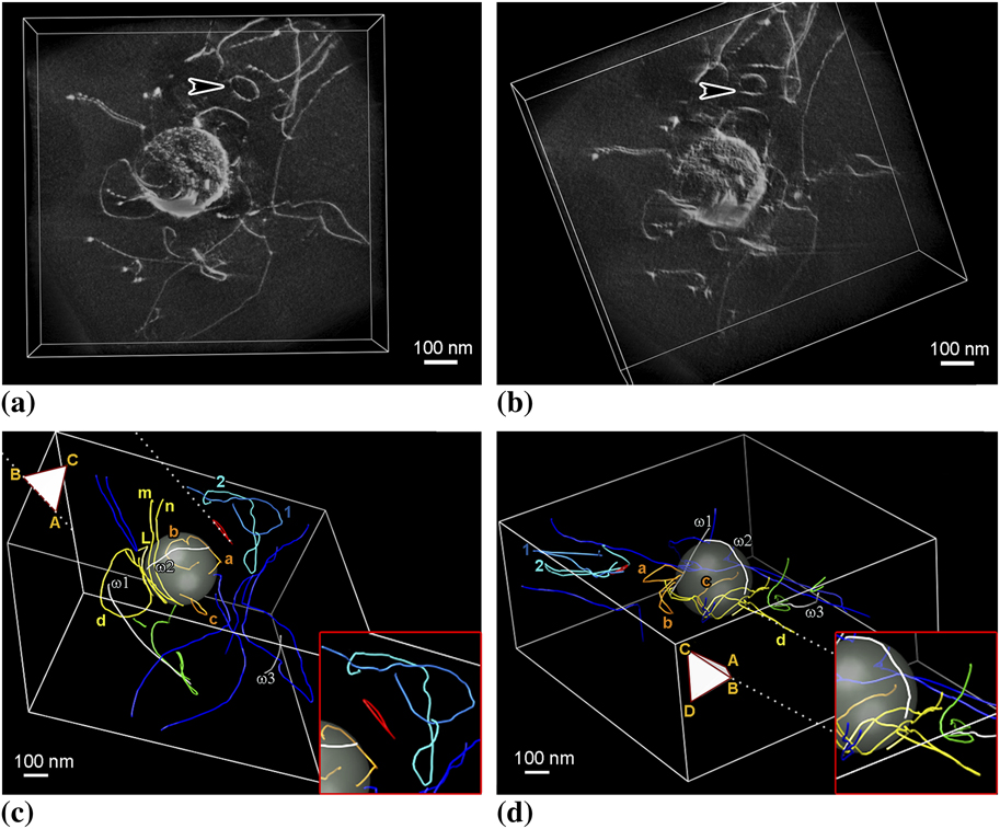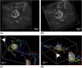4(c) and 4(d), have Burgers vectors of a / 2[101, a / 2[110] and as indicated. The images presented in Figs. 4(a) and 4(b) show views of the dislocation structure extracted from the tomographic reconstruction. Despite the image broadening and the corresponding decrease in the spatial resolution, the distribution of the dislocations around the particles is clear when compared with Figs. 3(a)–3(f). Dislocations bowing around the particle and dislocation loops attached to the particle can be seen; the arrowed prismatic loop was most likely released from the particle.

FIG. 3.

Dislocation structure produced around an Al₃Sc particle by deformation; the imaging condition was (g, 3g) using g = for (a)–(c) and g = 200 for (d)–(f). The arrows indicate tilt direction.

FIG. 4.

Spatial relationship between the dislocations and the particle. All colored dislocations have the same Burgers vector, b = ; dislocations traced in white have Burgers vectors from left: (ω1) b = a / 2[101], (ω2) b = , and (ω3) b = , respectively. (a) and (b) Views from different viewing directions extracted from the tomographic reconstruction. (c) and (d) Views from different viewing directions extracted from the three-dimensional (3D) model. Insets show enlargements of parts of the interactions.

The visualization of the dislocation structure and interactions can be further improved from the tomogram by effectively tracing the positions of the dislocation image using toolsets in UCSF Chimera. Here the dislocation position was assumed to be the region of highest intensity when viewed spatially. The positioning was verified by inspecting the traced images superimposed back onto the tomogram. It was found that the traced lines produced good matching from all viewing directions. That is, 3D dislocation positions are faithfully reproduced in the model. Examples of the dislocation structure and interactions as seen from different viewing directions are shown in the series of images presented in Figs. 4(c) and 4(d); enlargements of specific interactions, in particular, the slip plane of select defects with respect to the Thompson tetrahedron are shown in the insets.

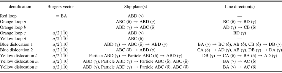
By using the tetrahedron included in these images, it is possible to specify which planes the various loops reside on. Table I lists the slip planes and line directions of the relevant dislocations. For example, in Figs. 4(c) and 4(d), the red loop detached from the particle has a Burgers vector of (BA) and resides on the ABD (or γ) plane. The orange loops labeled a and b attached to the particle surface lie on different planes, with loop a lying on the ABC (or δ) plane and b on the ABD (or γ) plane. Away from the particle surface, both loops cross slip such that loop a now resides on the γ-plane and loop b on the δ-plane. The Burgers vector of the loops, namely, is consistent with the common direction for the intersection of the δ-plane and γ-plane. It is believed that the loops cross-slipped as they extend away from the particle to glide on more energetically favorable slip planes. Orange loop, c, lies on the γ-plane, whereas the large yellow loop, d, resides on the δ-plane. To the authors’ knowledge, cross slip of dislocation half-loops, which themselves resulted from a previous interaction between matrix dislocations and the particle, from the particle–matrix interface has not been simulated, though abundant examples do exist suggesting a variety of possible dislocation debris structures as a result of such interactions.Reference Xiang, Srolovitz, Cheng and Weinan^4, Reference Xiang, Chang, Srolovitz and Weinan⁵

TABLE I.

Line directions and planes of the dislocation loops and lines shown in Figs. 4(c) and 4(d).

Identification of the true line direction of the dislocations, however, is more complex because the direction can change as the dislocation line stretches from the top to the bottom surface of the foil. For example, the blue dislocation segment labeled 2 has a Burgers vector b = and a line direction and slip plane that changes, from the side closest to the red loop, from CA (δ) → AD (γ) → AB (γ) → DB (γ) → DA (γ), indicating that it has cross-slipped as it approaches a foil surface. Dislocation 1 has the same Burgers vector and a line direction that changes from the side closest to the red loop from BA (γ) → BC (δ) → AB (δ) → CB (δ) → DB (γ). Since both 1 and 2 end on the same-side foil surface, it is suggested that they could have been loops similar to the red loop, which have grown large enough to eventually intersect the foil surface. The change in line direction as the surface is approached is consistent with the influence of surface image forces on the direction of the line dislocation.

Two dislocations labeled m and n in Fig. 4(c) curve around the particle, both have a Burgers vector of b = , reside mostly on the δ-plane, and change line direction as the foil surface is approached due to image forces. For both dislocations, the ends of the dislocations terminate on the same foil surface. Dislocation l, on the other hand, ends on the particle interface while conforming to the interface. This was not the case for any other dislocations in the current data set, though this is a common observation.

What is not known is how these dislocation interactions with the particle will continue with further deformation. It is possible for a portion of the dislocation conforming to the particle surface to pinch off, producing the partial-loop configurations similar to orange loops a and b, with the remaining segment extending from the matrix–particle interface to the free surface. Alternatively, the loops could cross-slip with pinch off occurring at the cross-slip point to release one loop from the particle and leave another tethered to it. The tethered loop may expand again under the influence of an applied load allowing the process to repeat or it could collapse onto the particle–matrix interface and be accommodated on the interface. Both release of loops from particle–matrix interfaces and collapse of half loops onto the interface have been observed during in situ TEM straining experiments.

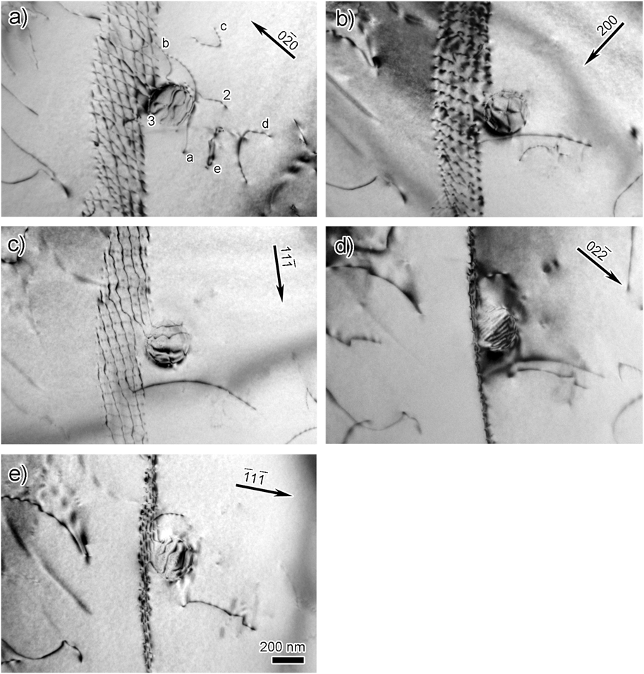
The previous example emphasized the interaction of individual dislocations with particles. However, interactions occurring between particles and sub-grain and grain boundaries are important in processes such as static and dynamic recrystallization, grain growth, superplasticity, etc. In situ TEM straining experiments at elevated temperatures show that the interaction between an array of dislocations and a large particle, one with interfacial dislocations, can involve the interaction of the array dislocations with interfacial ones.Reference Clark, Robertson, Dougherty, Ahn and Sofronis^2, Reference Dougherty, Robertson and Vetrano^3, Reference Dougherty⁷ Such interactions decreased the mobility of the array dislocations by about 30%, which was less than expected, and the array reformed after the interaction. The bright-field images taken with different diffraction vectors and presented in Fig. 5 show the later stages of an interaction of a twist-boundary with an Al₃Sc particle. Some dislocations from the array remain connected to the particle and dislocation lines and loops reside in the vicinity of it. This tethering of the boundary to the particle after an interaction is common.Reference Clark, Robertson, Dougherty, Ahn and Sofronis^2, Reference Dougherty⁷ From these images, the Burgers vector of the dislocations can be determined. The screw dislocations forming the boundary have Burgers vectors of either b = or b = , and dislocations with b = ±a / 2[010] form at the intersection nodes of the two screw dislocations.

FIG. 5.

Bright-field images taken with different diffraction vectors showing the dislocation arrangement of a twist boundary interacting with a Al₃Sc particle. The same dislocations as those shown in the reconstruction, Figs. 6(c)–6(e), are labeled for comparison.

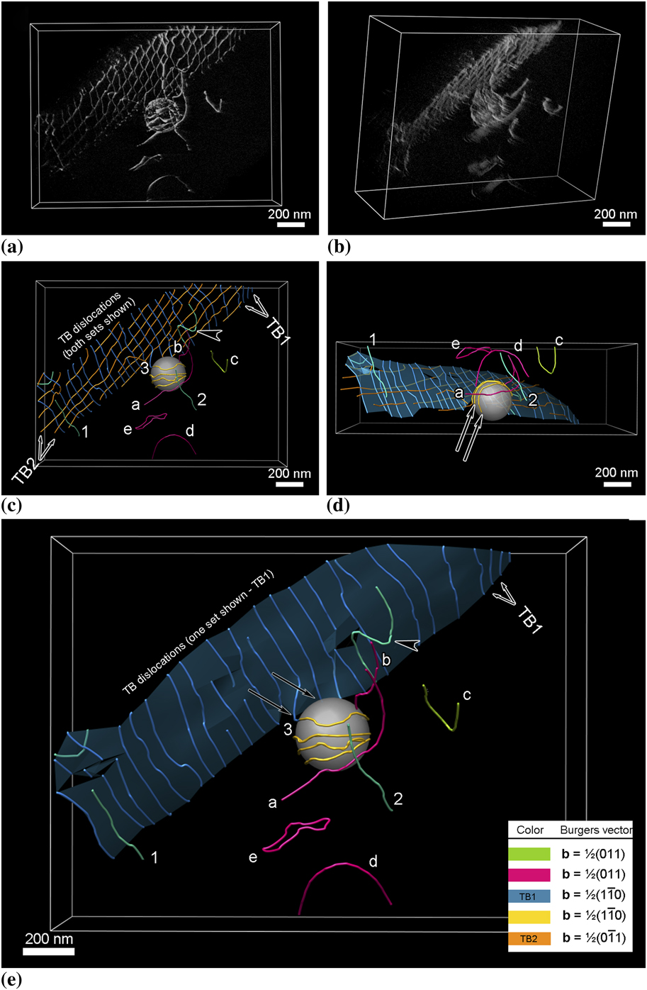
To show the dislocation arrangement, a weak-beam dark-field series of images was acquired over the angular range from −21.3° to +37.3° with the diffraction condition maintained with g = 020 and s_g = 6.7 × 10⁻³ Å⁻¹. These images were aligned into a stack, and supplemental movie file 2 shows a fly-through of this tilt-series. Using the same method for alignment and reconstruction, a tomogram and a 3D model were constructed and select images from different vantage points from both are shown in Fig. 6; in the case of the traced images, the junction reaction in the boundary plane was ignored for simplicity.

FIG. 6.

Spatial relationship between the twist boundary, the dislocations, and the particle. (a) and (b) Views from different directions extracted from the tomographic reconstruction. (c)–(e) Views from different directions extracted from the 3D model. In (c), both sets of dislocations in the twist boundary are shown, whereas in (e) one set is removed for clarity and shown with an overlay of the boundary. The “side view” shown in (d) is equivalent to a viewing direction perpendicular to the electron beam, which is normally inaccessible. The arrows indicate dislocations residing in the particle–matrix interface.

The first noticeable feature is that not all the dislocations that appear in the conventional micrographs as being part of the twist boundary actually reside on the boundary plane despite having the same Burgers vector as one of the dislocation sets that form the boundary. For example, dislocations 1 and 2 in Fig. 6(e) have a Burgers vector of b = , which is the same as the twist boundary dislocations labeled TB1 and colored blue. Certainly, dislocation 1 appears in the conventional electron micrographs to be an integral dislocation of the twist boundary—but from the tomogram it is clear that this is merely a projection effect. Additionally, the dislocation indicated by the arrowhead in Figs. 6c and 6e is part of the dislocation array but remains bowed out from the array plane, indicating that this particular dislocation may have interacted with the particle and has yet to realign with the other dislocations. Alternatively, it is possible, although not verified in this case, that this dislocation is in the process of detaching from the array. This ejection of dislocations from the twist boundary may explain the origin of dislocations 1 and 2, which may indicate the instability of this boundary after it has interacted with the particle.

One boundary dislocation, 3, appears to remain attached to the particle and to have formed a partial loop around the particle, before appearing to terminate on the particle–matrix interface. However, as the angular tilt range was not sufficient to “see” behind the particle, the actual termination point of this dislocation could not be determined unequivocally. Dislocation lines a and b, partial loops c and d, and full loop e have a Burgers vector of b = ±a / 2[011] and reside on different planes. Line dislocation b extends from the particle surface to the free surface, whereas dislocation a extends through the foil and interacts with the particle as evidenced by its curvature. Partial loops c and d reside on the α-plane, although there is some distortion as the free surface is approached; such distortions are expected from consideration of surface image force effects on line dislocations. It should be noted that as the tomogram is formed with only one excited reflection, 020 in this instance, dislocations with a Burgers vector of either b = or b = ±a / 2[101] are invisible and this can lead to misinterpretation of tomographic images in a similar manner as it would in conventional micrographs. For example, the complete loop e appears to lie on two different planes, the lower portion resides on the β-plane but the upper portion does not coincide with an allowed plane. From bright-field images formed with different diffraction vectors, two additional dislocations, one with a Burgers vector of b = ±a / 2[101] and the other with b = , intersect the loop at the two locations at which it is kinked. These interactions yield segments with Burgers vectors of b = and b = ±a / 2[110], respectively. These reactions are consistent with the Burgers vector analysis using the images presented in Fig. 5. These interactions account for the observed form of this dislocation loop. Thus, it is possible to specify in detail the configuration of the dislocations interacting with and in the vicinity of the particle.