


1. Introduction
Turbulent convection is ubiquitous in nature and in many industrial processes. Examples include the convective flows in the Earth's mantle (Mckenzie, Roberts & Weiss Reference Mckenzie, Roberts and Weiss1974) and outer core (Cardin & Olson Reference Cardin and Olson1994), in the atmospheric motion (Wyngaard Reference Wyngaard1992; Hartmann, Moy & Fu Reference Hartmann, Moy and Fu2001), in the ocean (Cheng et al. Reference Cheng, Abraham, Hausfather and Trenberth2019) and in rotational machines (Michael Owen & Long Reference Michael Owen and Long2015). Many of these convection phenomena occur under rapid rotation of the system (Bohn et al. Reference Bohn, Deuker, Emunds and Gorzelitz1995). Rayleigh–Bénard convection (RBC), a fluid layer heated from below and cooled from above, is a classical and idealized paradigm for the study of thermally driven turbulent flows (Ahlers, Grossmann & Lohse Reference Ahlers, Grossmann and Lohse2009; Lohse & Xia Reference Lohse and Xia2010; Chillà & Schumacher Reference Chillà and Schumacher2012; Xia Reference Xia2013; Yu et al. Reference Yu, Liu, Zhou, Gao and Liu2019; Zou et al. Reference Zou, Zhou, Chen, Bao, Chen and She2019; Chen, Wang & Xi Reference Chen, Wang and Xi2020; Wang et al. Reference Wang, Jiang, Jiang, Sun and Liu2021). The main issues for thermal turbulence studies include the dynamics of turbulent structures and the scaling relation between the heat transport, in the dimensionless form, Nusselt number  $Nu$, and thermally driven force, in the dimensionless form, Rayleigh number
 $Ra$. Recently a novel system similar to classical RBC, an annular centrifugal RBC (ACRBC) system with cold inner and hot outer cylinders corotating axially, has been proposed (Kang et al. Reference Kang, Meyer, Yoshikawa and Mutabazi2019; Jiang et al. Reference Jiang, Zhu, Wang, Huisman and Sun2020; Rouhi et al. Reference Rouhi, Lohse, Marusic, Sun and Chung2021). By exploiting strong centrifugal force through rapid rotation, the intensity of the thermal driving can be significantly enhanced.
In ACRBC, Jiang et al. (Reference Jiang, Zhu, Wang, Huisman and Sun2020) found that the convective rolls revolve around the rotating centre in the prograde direction, signifying the emergence of zonal flow, which may be related to the effects of Coriolis force and the different curvatures of the two cylinders. In the atmospheric sciences and dynamical systems communities, a flow in the azimuthal direction is observed in the rotating cylindrical annulus, which is attributed to the baroclinic instability (Fowlis & Hide Reference Fowlis and Hide1965; Williams Reference Williams1971; Read & Risch Reference Read and Risch2011; Read et al. Reference Read, Morice-Atkinson, Allen and Castrejón-Pita2017). The Earth's gravity and rotation both play key roles in the baroclinic waves. In astrophysical and geophysical studies, by using a rotating cylindrical annulus with conical end surfaces, Busse and his collaborators (Busse & Carrigan Reference Busse and Carrigan1974; Azouni, Bolton & Busse Reference Azouni, Bolton and Busse1985; Busse & Or Reference Busse and Or1986; Busse Reference Busse1994) also observed a zonal flow phenomenon. According to the topographic- $\beta$ approximation (Yano, Talagrand & Drossart Reference Yano, Talagrand and Drossart2005), the strength and direction of the zonal flow in their system depend on the radial gradient of the axial fluid column height. By using a spherical shell model with a radius ratio of 0.9, Heimpel, Aurnou & Wicht (Reference Heimpel, Aurnou and Wicht2005) found that zonal flow in the equatorial latitude of Jupiter is prograde with respect to the planet, which is consistent with the actual observed results of Jupiter (Porco et al. Reference Porco2003), but the width of equatorial zonal flow does not coincide with the predictions of Rhines scale (Rhines Reference Rhines1975). The physical mechanism of zonal flow in ACRBC and how it is affected by the curvatures of the two cylinders (Jiang et al. Reference Jiang, Zhu, Wang, Huisman and Sun2020) deserves further study.
In classical turbulent RBC, the effects of aspect ratio  $\varGamma$ on the Nusselt number
 $Nu$ have been extensively studied (Sun et al. Reference Sun, Ren, Song and Xia2005; Ahlers et al. Reference Ahlers, Grossmann and Lohse2009; van der Poel, Stevens & Lohse Reference van der Poel, Stevens and Lohse2011; Huang et al. Reference Huang, Kaczorowski, Ni and Xia2013; Huang & Xia Reference Huang and Xia2016) and it is found that heat transport efficiency has a great relevance on
 $\varGamma$ when it is smaller than 1 (van der Poel et al. Reference van der Poel, Stevens and Lohse2011). Huang et al. (Reference Huang, Kaczorowski, Ni and Xia2013) and Huang & Xia (Reference Huang and Xia2016) investigated the effects of lateral confinement on heat transport in quasi-two-dimensional (quasi-2-D) turbulent RBC and found that the narrow lateral width of the convection cell induces the increase of the heat transfer efficiency. In high-Reynolds number Taylor–Couette (TC) turbulence, Grossmann, Lohse & Sun (Reference Grossmann, Lohse and Sun2016) analysed multiple sets of data from the previous experiments and direct numerical simulations (DNS), and found that in the range of radius ratio 0.5–0.909, as the radius ratio increases, the amplitude of TC Nusselt number
 $Nu_\omega$ (the dimensionless angular velocity flux) first increases, and then saturates when the radius ratio is greater than 0.7, indicating that larger radius ratio can achieve higher momentum transport efficiency. Therefore, it is of vital importance to study the effects of geometry on the heat transport efficiency of the ACRBC system, and it can also give insights for the design of rotating machinery (King, Wilson & Owen Reference King, Wilson and Owen2005; Pitz et al. Reference Pitz, Chew, Marxen and Hills2017a; Chalghoum et al. Reference Chalghoum, Elaoud, Kanfoudi and Akrout2018).
We notice that Pitz, Marxen & Chew (Reference Pitz, Marxen and Chew2017b) and Kang et al. (Reference Kang, Meyer, Yoshikawa and Mutabazi2019) have studied the effects of the radius ratio on the centrifugal buoyancy driven flow, but they mainly focused on the dependence of the critical Rayleigh number  $Ra_c$ and the critical wavenumber
 ${\omega _c}$ of convection onset through linear stability analysis and numerical simulation. For higher Rayleigh number
 $Ra$ in the turbulent regime, to the best of our knowledge little attention has been paid to systematically studying the effects of radius ratio. To fill this gap, we present a systematic investigation of the dynamics of zonal flow and heat transfer properties in the turbulent regime of the ACRBC system with radius ratio from 0.3 to 0.9 by means of three-dimensional (3-D) DNS. Will the geometric effects in ACRBC be similar to those in RBC or in TC? Answering this question is the major objective in this study.
The remainder of this manuscript is organized as follows. In § 2, we give a brief description of the governing equations and the numerical model. The results are presented and analysed in § 3, which is divided into three parts. Section 3.1 describes the dynamics of zonal flow in ACRBC and explains the physical mechanism of it. In § 3.2, we show the dependence of heat transfer on radius ratio, and discuss the physical reasons. Remarkably asymmetric mean temperature fields are found in ACRBC and predicted by a theoretical model, which is discussed in § 3.3. Finally, we summarize our findings in § 4.
2. Numerical settings
2.1. Flow set-up
We consider a fluid bounded by cold inner and hot outer cylinders, which corotate axially as shown in figure 1. The governing equations are derived from the Navier–Stokes equations under the Boussinesq approximation in a rotating reference frame (the detailed derivation of the non-dimensional governing equations is provided in the Appendix A), which are expressed as
 $$\begin{gather} \boldsymbol{\nabla} \boldsymbol{\cdot} \boldsymbol{u} = 0, \end{gather}$$
 $$\begin{gather}\frac{{\partial \theta }}{{\partial t}} + \boldsymbol{u} \boldsymbol{\cdot} \boldsymbol{\nabla} \theta = \frac{1}{\sqrt{RaPr}}{{\nabla}^2}\theta, \end{gather}$$
 $$\begin{gather}\frac{{\partial \boldsymbol{u}}}{{\partial t}} + \boldsymbol{u} \boldsymbol{\cdot} \boldsymbol{\nabla} \boldsymbol{u} ={-} \boldsymbol{\nabla} p - Ro^{ - 1} \boldsymbol{\widehat \omega} \times \boldsymbol{u} + \sqrt \frac{{Pr}}{{Ra}} {{\nabla}^2} \boldsymbol{u} - \theta \frac{{2(1 - \eta )}}{{(1 + \eta )}} \boldsymbol{r}, \end{gather}$$
where  $\boldsymbol {\widehat \omega }$ is the unit vector pointing in the direction of the angular velocity,
 $\boldsymbol {u}$ is the velocity vector normalized by the free-fall velocity
 $U \equiv \sqrt {{\omega ^2}({{({R_o} + {R_i})}}/{2})\alpha \varDelta L}$,
 $t$ is the dimensionless time normalized by
 $L/U$, and
 $\theta$ is the temperature normalized by
 $\varDelta$. Here, as defined in figure 1,
 $\omega$ denotes the angular velocity of the system. Here
 ${R_o}$ and
 ${R_i}$ are the radius of the outer and inner cylinders, respectively,
 $\alpha$ is the isobaric thermal expansion coefficient of the fluid,
 $\varDelta$ and
 ${L}$ are the temperature difference (
 $\varDelta \equiv {\theta _{hot}} - {\theta _{cold}}$) and the gap (
 $L \equiv {R_o} - {R_i}$) between the two cylinders. In the coordinate system
 $\phi$,
 $z$,
 $r$ refer to the streamwise (azimuthal), spanwise (axial) and wall-normal (radial) directions. In the following, we will adopt
 $R^{\prime } = (R - {R_i})/({R_o} - {R_i})$ as the radial position to unify the cases with different
 $\eta$.
Schematic diagram of the flow configuration. Here  $\omega$ is the angular velocity of the system. All cases in this paper set the angular velocity unit vector
 $\boldsymbol {\widehat \omega } = +1$, that is, the system rotates anticlockwise. Here
 ${R_o}$,
 ${R_i}$,
 $H$ and
 $L$ are the inner radius of the outer cylinder, the outer radius of the inner cylinder, the height of the cylindrical annulus, and the gap width between the two cylinders, respectively. Here
 ${\theta _{hot}}$ and
 ${\theta _{cold}}$ denote the temperature of the outer and inner walls.

The above dimensionless governing equations reveal that ACRBC is mainly controlled by four dimensionless parameters. Similar to classical RBC, the Rayleigh number is defined as
 \begin{equation} Ra = \tfrac{1}{2}{\omega^2}({R_o} + {R_i})\alpha \varDelta {L^3}/(\nu \kappa), \end{equation}
and Prandtl number as  $Pr = \nu /\kappa$, which characterize the buoyancy-driven strength and physical properties of the convecting fluid. Here,
 $\nu$ and
 $\kappa$ are the kinematic viscosity and thermal diffusivity of the fluid, respectively. Note that the centrifugal term
 $- \theta ({{2(1 - \eta )}}/{{(1 + \eta )}})\boldsymbol {r}$ grows linearly with the radius, which is consistent with reality. While the characteristic value of centrifugal force is
 ${\omega ^2}({R_i} + {R_o})/2$, which is used in the definition of free-fall velocity
 $U$ and
 $Ra$. Two additional control parameters are
 ${Ro^{-1}} = \omega L/U$ and
 $\eta = {R_i}/{R_o}$, which measure Coriolis force effects and geometric properties. The key response parameter is the Nusselt number given by
 \begin{equation} Nu = \frac{J}{{{J_{con}}}} = \frac{{{{\left\langle {{u_r}\theta} \right\rangle }_{\phi ,z,t}} - \kappa \dfrac{\partial }{{\partial r}}{{\left\langle \theta \right\rangle }_{\phi ,z,t}}}}{{\kappa \varDelta {{(r \cdot \ln(\eta ))}^{{-}1}}}}, \end{equation}
where  $J$,
 ${{J_{con}}}$,
 ${u_r}$ and
 $\theta$ denote the total heat flux, the heat flux through pure thermal conduction and the radial velocity and temperature of a certain point, respectively. Here
 ${\langle {\cdots } \rangle _{\phi,z,t}}$ denotes taking the average over the
 $\phi z$-plane and time. The derivation of conductive heat flux in cylindrical geometry is slightly different from that in classical RBC, and the derivation of (2.5) is supplied in Appendix B.
2.2. DNS
Numerical simulations are performed using an energy-conserving second-order finite-difference code, which has been described in detail in the literature (Verzicco & Orlandi Reference Verzicco and Orlandi1996; van der Poel et al. Reference van der Poel, Ostilla-Mónico, Donners and Verzicco2015a; Zhu et al. Reference Zhu2018; Jiang et al. Reference Jiang, Zhu, Wang, Huisman and Sun2020). Thus, here we introduce it briefly and just give some main features. Table 1 in Appendix C lists all the specific simulation parameters. For all cases, no-slip boundary conditions for velocity and constant temperature boundary conditions are adopted at the surfaces of the inner and outer cylinders, which is different from the free-slip boundary conditions in Goluskin et al. (Reference Goluskin, Johnston, Flierl and Spiegel2014), von Hardenberg et al. (Reference von Hardenberg, Goluskin, Provenzale and Spiegel2015) and Wang et al. (Reference Wang, Chong, Stevens, Verzicco and Lohse2020). Thus, zonal flow in our system is much weaker and more similar to laboratory conditions. Periodic boundary conditions are imposed on  $\boldsymbol {u}$ and
 $\theta$ in the
 $z$-direction. The aspect ratio (
 $\varGamma = H/L$) for most cases is set
 $\varGamma = 1$, but for high
 $Ra$ cases (i.e.
 $Ra > {10^7}$),
 $\varGamma$ is reduced to 0.5 and in several cases to 0.25. Furthermore, for large
 $Ra$ and
 $0.6 \le \eta \le 0.9$, the azimuthal domain is reduced from a whole circle (
 ${\phi _0} = 1$) to
 ${\phi _0} = 1/2, 1/4, 1/8$. The flow domain at least contains a pair of convection rolls to ensure the statistical stability. It is found that such an arrangement will not have a considerable impact on
 $Nu$ and zonal flow.
Adequate resolutions are ensured for all simulations and we have performed a posteriori checks of spatial and temporal resolutions to guarantee to resolve all relevant scales. As shown in table 1, the ratio of maximum grid spacing  ${\varDelta _g}$ in the bulk region to the Kolmogorov scale estimated by the global criterion
 ${\eta _K} = {{L{{Pr }^{1/2}}}}/{{[{Ra(Nu - 1)}]}^{1/4}} \cdot {[{{(1 + \eta )\ln (\eta )}}/{{2(\eta - 1)}}]^{1/4}}$ (Jiang et al. Reference Jiang, Zhu, Wang, Huisman and Sun2020) is smaller than 0.7 (
 ${\varDelta _g}/{\eta _K} < 0.7$). We have also compared
 ${\varDelta _g}$ with the Batchelor scale
 ${\eta _B} = {\eta _K}{Pr^{ - 1/2}}$ (Silano, Sreenivasan & Verzicco Reference Silano, Sreenivasan and Verzicco2010) for each case (not shown here) and we have
 ${\varDelta _g}/{\eta _B} < 1.4$. Furthermore, the clipped Chebychev-type clustering grids adopted in the radial direction ensure the spatial resolution within boundary layers (BLs). There are at least eight grid points inside thermal BLs and 10 grid points inside viscous BLs. We use the Courant–Friedrichs–Lewy (CFL) conditions to check temporal resolution (Courant, Friedrichs & Lewy Reference Courant, Friedrichs and Lewy1928; van der Poel et al. Reference van der Poel, Ostilla-Mónico, Donners and Verzicco2015a; Zhang, Zhou & Sun Reference Zhang, Zhou and Sun2017), i.e. the CFL number is smaller than 0.8 for all simulations to ensure computational stability. Here
 ${\tau _{avg}}$ is the averaging time for the Nusselt number. For simulation convergence, each case is run for approximately 100 free-fall time units to discard initial transients, and we obtain the
 $Nu$ by averaging over an additional
 ${\tau _{avg}} \ge 80$ and over the Nusselt numbers at the inner (
 $Nu_{in}$) and outer (
 $Nu_{out}$) walls. One way for statistical convergence is when the difference of the
 $Nu$ between inner and outer walls
 ${\epsilon _{Nu}} = | Nu_{in} - Nu_{out} |/Nu$ is small and acceptable (Ostilla et al. Reference Ostilla, Stevens, Grossmann, Verzicco and Lohse2013; Kunnen et al. Reference Kunnen, Ostilla-Mónico, van der Poel, Verzicco and Lohse2016). For most cases,
 ${\epsilon _{Nu}}$ is less than
 $1\,\%$ and the maximum of
 ${\epsilon _{Nu}}$ is approximately
 $1.73\,\%$, as shown in table 1.
2.3. Explored parameter space
In the present study, we aim at studying the geometric effects on ACRBC systematically. The simulations cover a radius ratio  $\eta$ range [0.3, 0.9] and a
 $Ra$ range [
 ${10^6}$,
 ${10^8}$]. Here
 $Pr$ is fixed at 4.3, corresponding to the working fluids of water at
 ${40}\,^{\circ }\mathrm {C}$. Also,
 $Ro^{- 1}$ is fixed at 1, that is because when
 $Ro^{ - 1} \ll 1$, the rotation effect is too weak; while when
 $Ro^{ - 1} \gg 1$, the turbulence is suppressed, and the flow becomes quasi-2-D state. From the previous tests, we find that zonal flow is strong at
 $Ro^{ - 1} = 1$ and
 $Pr = 4.3$. For fixed
 $Ro^{ - 1} = 1$, the influence of rotation (Coriolis force) remains comparable for all values of the buoyancy forcing (
 $Ra$). We concentrate on the
 $\eta$ effects on the flow structure and heat transport for different
 $Ra$ while the time scales of rotation and convective motion are similar. Besides, all the results in this paper set the angular velocity unit vector
 $\boldsymbol {\widehat \omega } = +1$, that is, the system rotates anticlockwise.
3. Results and discussion
3.1. Zonal flow
As mentioned in Jiang et al. (Reference Jiang, Zhu, Wang, Huisman and Sun2020), the convection rolls in ACRBC revolve in the prograde direction around the axis with a faster rotation rate than the background rotation of the experimental system, which is the so-called zonal flow. The mechanisms of zonal flow and the responses of the dynamics of zonal flow to  $\eta$ and
 $Ra$ are discussed in § 3.1.1. Next we present some statistical analyses of zonal flow, i.e. the frequency
 ${\omega _d}$ of the net rotation of the convection rolls and the strength of zonal flow
 $\langle {{u_\phi }} \rangle _{V,t}$ in § 3.1.2, where
 ${\langle {\cdots } \rangle _{V,t}}$ denotes the average over the whole volume and time.
3.1.1. Dynamics of zonal flow
Akin to the classical RBC, the direction of the temperature gradient is parallel to the centrifugal buoyancy in ACRBC. As the temperature difference or the rotation rate increases, the flow will gradually become unstable and convection appears when  $Ra$ is higher than critical
 $Ra_{c}$ (Pitz et al. Reference Pitz, Marxen and Chew2017b) of convection onset. When
 $Ra \gtrsim {10^6}$ (Kang et al. Reference Kang, Meyer, Yoshikawa and Mutabazi2019), the flow transitions to become turbulent in the bulk and we will focus on the turbulent convection regime.
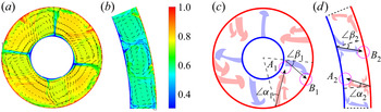
In the rotating reference frame, the Coriolis force emerges and plays an important role. As shown in figure 2, driven by the Coriolis force, the cold and hot plumes should both have deflected to the right-hand side from the initial direction. The initial deflected angle of hot plumes ( $\angle \alpha$) is roughly equal to the deflected angle of cold plumes (
 $\angle \beta$). As
 $Ro^{-1} = 1$, the Coriolis force balances inertial force and the flow is in the inertial regime. We also calculate the root-mean-square axial velocity
 ${\langle {{{({u_z})}_{rms}}} \rangle _{r,\phi,z}}$ for different
 $\eta$ and
 $Ra$. It is found that
 ${\langle {{{({u_z})}_{rms}}} \rangle _{r,\phi,z}} \sim 0.025$ at
 $Ro^{-1} = 1$, which is much larger than that in the quasi-2-D state (see figure 2D of Jiang et al. (Reference Jiang, Zhu, Wang, Huisman and Sun2020)). So the flow is still quite 3-D and not in geostrophic balance (Coriolis
 $\sim$ pressure). In the inertial regime, the plumes should be deflected by the Coriolis force to roughly follow ‘inertial circles’ (Cushman-Roisin & Beckers Reference Cushman-Roisin and Beckers2011). We define the radius of the inertial circle as
 $\widehat R$. According to the balance relation between the inertial force and Coriolis force,
 $(U/\widehat R)U \sim 2\omega U$, then the flow would deflect with a radius of curvature
 $\widehat R = U/(2\omega )$. The ejection velocity of cold plumes is larger than that of hot plumes, which would cause the radius of curvature of the trajectory circle
 $\widehat R = U/(2\omega )$ of cold plumes to be larger (see figure 2a,c). The asymmetric trajectory of plumes leads to the generation of zonal flow.
Typical snapshots of instantaneous temperature fields, superposed by the velocity vectors for (a)  $\eta = 0.4$ and (b)
 $\eta = 0.9$ at
 $Ra = {10^7}$,
 $Ro^{ - 1} = 1$ and
 $Pr = 4.3$. To visualize the plumes clearly, the temperature colourbar is from 0.3 to 1. (c,d) Corresponding sketches to panels (a,b), which show the motions of cold (blue) and hot (red) plumes. Here
 $\angle \alpha$ and
 $\angle \beta$ are the deflected angle of the hot and cold plumes, respectively. Here
 $A$ and
 $B$ are the impacting region of the hot and cold plumes, respectively. The arrows show the trajectory of the plumes.

The reason for the larger ejection velocity of cold plumes is estimated from the expression of local free-fall velocity and verified from the numerical results. The local free-fall velocity  $U \equiv \sqrt {({\omega ^2}R)\alpha \varDelta L}$. On the one hand, from the local temperature difference aspect, the temperature difference near the inner cylinder is larger than that near the outer cylinder because
 ${\theta _m} < {\theta _c}$ (This point will be discussed in § 3.3). On the other hand, supergravity(
 ${\omega ^2}R$) is stronger near the outer cylinder. For example, for
 $\eta = 0.5$,
 $$\begin{gather} {\varDelta_{inner}} = |{\theta_{inner}} - {\theta_c}| \sim 0.75 \varDelta, \quad {\varDelta_{outer}} = |{\theta_{outer}} - {\theta_c}| \sim 0.25 \varDelta, \end{gather}$$
 $$\begin{gather}\frac{{{U_{inner}}}}{{{U_{outer}}}} = \frac{{\sqrt {({\omega^2}{R_{inner}})\alpha {\varDelta_{inner}}L} }}{{\sqrt {({\omega^2}{R_{outer}})\alpha {\varDelta_{outer}}L} }} \sim \sqrt {\frac{3}{2}} \approx 1.22. \end{gather}$$
Therefore, the deflection angle of the cold plumes at the inner boundary is smaller because the local radius of curvature  $\widehat R = U/2\omega$ is larger. Further, we compare the radial velocity
 $|{u_r}|$ of the cold plumes and hot plumes. Because the strength of zonal flow is relatively strong at
 $Ra = 10^7$, we study the radial velocity
 $|{u_r}|$ versus
 $\eta$ at
 $Ra = 10^7$. According to the azimuthal distribution of the radially and axially averaged radial velocity
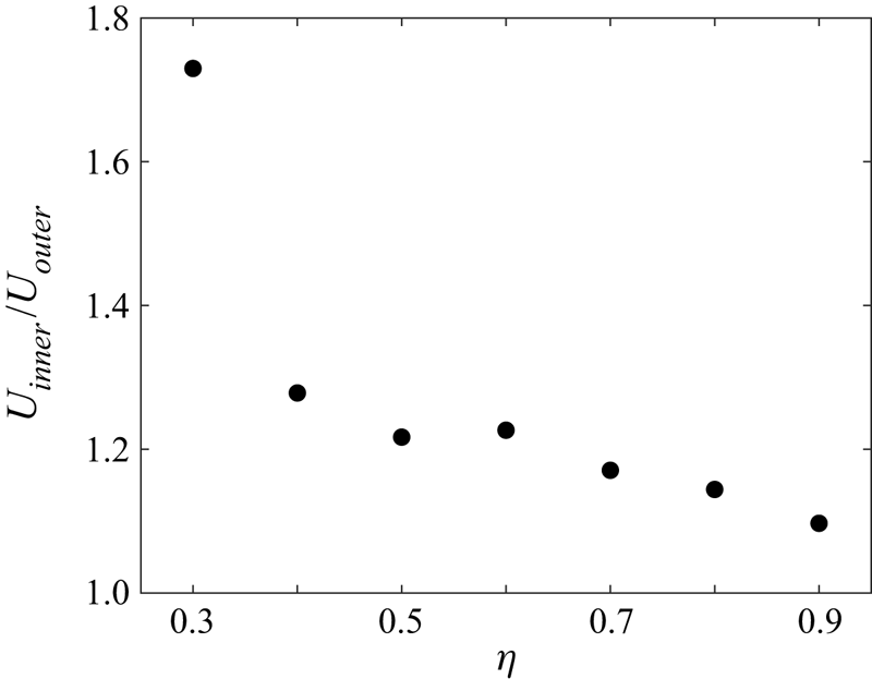
 ${{{\langle {{u_r}} \rangle }_{r,z}}}$, we can detect the positions of the cold and hot plumes. The velocities of plumes are then averaged by time (20 free-fall time units, 0.2 time interval) and each roll. As shown in figure 3, cold plumes have a larger local velocity than hot plumes. The ratio of local velocity for cold plumes
 $|{u_{r,c}}| = {U_{inner}}$ to local velocity for hot plumes
 $|{u_{r,h}}| = {U_{outer}}$ decreases with
 $\eta$ increasing, which is consistent with the trend of zonal flow strength versus
 $\eta$ (discussed in § 3.1.2).
The ratio of local velocity for cold plumes to local velocity for hot plumes  ${U_{inner}}/{U_{outer}}$ as a function of
 $\eta$ at
 $Ra = {10^7}$.

Next, we provide the second mechanism of the generation of zonal flow. Because of the different curvatures of the inner and outer cylinders (see figure 2a,c),  $\eta = 0.4$), the hot plumes deflect and then impact on
 ${A}_1$, which is close to the region where the cold plumes are ejected, whereas the distance between the impacting region
 ${B}_1$ of the cold plumes and the emitting region of hot plumes is relatively large. Consequently, the hot plumes ‘win’ and push the overall flow to move anticlockwise. Some cold plumes even deflect to the left-hand side due to the impact of hot plumes. For comparison, the difference between the curvatures of the hot and cold walls is small at
 $\eta = 0.9$ (see figure 2b,d) and both the impacting regions
 ${A}_2$ and
 ${B}_2$ are far away from the ejecting positions of cold and hot plumes, respectively. Thus, zonal flow becomes weaker with
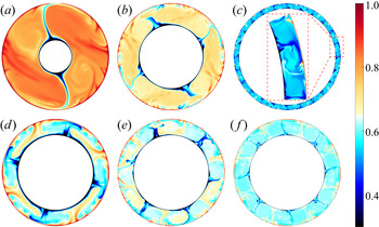
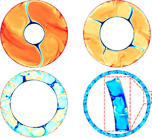
 $\eta$ increasing. Note that this mechanism of the zonal flow is different from the ‘inertial circle’ theory. Even though the radius of curvature of the trajectories of cold and hot plumes are the same, plume impingement will also occur. Figure 4(a–c) shows the instantaneous temperature fields for different radius ratios
 $\eta$ at
 $Ra = {10^7}$. When
 $\eta = 0.3$ (figure 4a, also see supplementary movie 1 available at https://doi.org/10.1017/jfm.2021.889), the deflected distances of hot plumes are remarkably larger than the cold plumes. When
 $\eta = 0.6$ (figure 4b, also see supplementary movie 2), the asymmetric movements of cold and hot plumes still could not be ignored. Hot plumes can impact on the root region of the cold plumes, but on the contrary the impacting region of cold plumes cannot affect the hot plumes directly. When
 $\eta = 0.9$ (figure 4c, also see supplementary movie 3), the movements of cold and hot plumes are almost symmetric, and there are several pairs of LSC rolls without distinct azimuthal movement, which is similar to the classical RBC.
(a–c) Instantaneous temperature fields on a  $\phi r$-plane for
 $\eta$ = 0.3, 0.6, 0.9 at
 $Ra = {10^7}$,
 $Ro^{ - 1} = 1$ and
 $Pr = 4.3$. (d–f) Instantaneous temperature fields for
 $Ra = {10^6}$,
 ${10^7}$,
 ${10^8}$ at
 $\eta = 0.7$,
 $Ro^{ - 1} = 1$ and
 $Pr = 4.3$. To visualize the plumes clearly, the temperature colourbar is from 0.3 to 1. All figures share the same colourbar.

Figure 4(d–f) demonstrates the influences of  $Ra$ on flow structures for
 $\eta = 0.7$. As we know, for classical RBC the aspect ratio of convection rolls is approximately equal to one without the confinement effects of sidewalls, which is almost consistent with the case of
 $Ra = {10^8}$ in ACRBC (see figure 4f). However, we find that the wavenumber decreases with the decrease of
 $Ra$. This is because with the increase of
 $Ra$, the flow is more turbulent and the thermal BLs become more unstable. There are more thermal plumes detaching from the BLs and more convection rolls are formed. As shown in figure 5, it is indicated that the number of roll pairs
 $N$ is smaller than the circular roll hypothesis (Pitz et al. Reference Pitz, Marxen and Chew2017b),
 $\eta = (2N - {\rm \pi})/(2N + {\rm \pi})$, for almost all cases. The convection rolls are probably elongated by strong zonal flow. At
 $Ra = {10^6}$ or small
 $\eta$,
 $N$ is much smaller than the theoretical line, which is consistent with the strong zonal flow in this
 $Ra$ and
 $\eta$ regime.
Radius ratio  $\eta$ as a function of the number of roll pairs
 $N$ for different
 $Ra$. The solid line is the circular roll hypothesis as zonal flow is weak.

3.1.2. Quantitative analysis of zonal flow
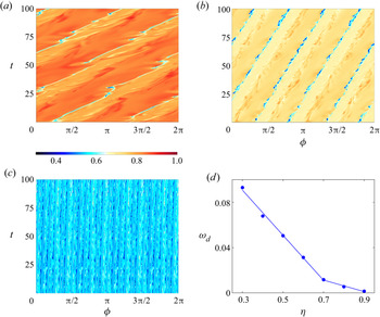
Figure 6(a–c) give the azimuth-time temperature contours at the midradius and midheight position for  $\eta = 0.3$, 0.6 and 0.9, respectively, which show that the convection rolls revolve in the prograde direction. And besides, the convection rolls drift at a nearly constant rate with high frequency oscillations. Similar effects have also been reported in Pitz et al. (Reference Pitz, Marxen and Chew2017b). Figure 6(d) suggests that the drift frequency
 ${\omega _d}$ decreases with
 $\eta$ increasing (averaged over 100 free-fall time units), where
 ${\omega _d}$ is defined as the azimuthal movement (radians) of convection rolls per free-fall time unit in the rotating frame. It is found that
 ${\omega _d} = - 0.05\eta + 0.05$ for
 $0.7 \le \eta \le 0.9$, while it gives a notably steeper slope with
 ${\omega _d} = - 0.2\eta + 0.15$ for
 $0.3 \le \eta \le 0.7$. This change of the slope of
 ${\omega _d}$ versus
 $\eta$ indicates that the influence of curvature effects on the drift frequency of convection rolls is more significant at small
 $\eta$.
Azimuth-time temperature contours at the midradius and midaxial position for (a)  $\eta = 0.3$, (b)
 $\eta = 0.6$ and (c)
 $\eta = 0.9$ at
 $Ra = {10^7}$. To visualize the plumes clearly, the temperature colourbar is from 0.3 to 1. All temperature fields share the same colourbar. (d) Drift frequency
 ${\omega _d}$ of the convection rolls versus
 $\eta$ at
 $Ra = {10^7}$, where
 ${\omega _d}$ is the drift angle (radians) per dimensionless time t. The solid lines are the best linear fits of
 ${\omega _d}(\eta )$ for
 $0.3 \le \eta \le 0.7$ and
 $0.7 \le \eta \le 0.9$, respectively.

Since that when there are no systematic deflections of plumes, one would expect that  ${\langle {{u_\phi }} \rangle _{\phi,z,t}}$ vanishes. Now
 ${\langle {{u_\phi }} \rangle _{\phi,z,t}}$ can reflect the asymmetric extent of the motion of cold and hot plumes. As shown in figure 7(a), with the decrease of
 $\eta$, the positive
 ${\langle {{u_\phi }} \rangle _{\phi,z,t}}$ (reflects the deflection of hot plumes) is larger and the negative part (reflects the deflection of cold plumes) is smaller in absolute value. We calculate the Reynolds stress
 ${\langle {u_\phi ^\prime u_r^\prime } \rangle _{\phi,z,t}}$ and find that the Reynolds stress is negative along the radius, which possibly results from the tilted plumes. Negative
 $\phi$-momentum is transported in the positive
 $r$-direction and positive
 $\phi$-momentum is transported in negative
 $r$-direction. Thus a strong prograde zonal flow develops in the inner part of the annulus. Figure 7(b) shows that, basically, for each fixed
 $Ra$, space- and time-averaged azimuthal velocity all decrease as
 $\eta$ increases. Thus, the drift of LSC rolls is directly linked to the asymmetric motion of cold and hot plumes. In addition, we find that at moderate
 $Ra$ (
 $Ra = {10^7}$), zonal flow is the strongest. When
 $Ra = {10^6}$, the velocity of plumes is slow due to the weak buoyancy (relative to viscosity); while when
 $Ra = {10^8}$, the flow is more turbulent and the coherent length of plumes decreases. So the zonal flow driven by the plumes for both cases is relatively weak. We also note that when
 $\eta \lesssim 0.5$ for
 $Ra = {10^6}$ and
 ${10^7}$ or
 $\eta \lesssim 0.4$ for
 $Ra = {10^8}$ (figure 7b),
 ${\langle {{u_\phi }} \rangle _{V,t}}$ no longer increases remarkably as
 $\eta$ decreases, which is probably a consequence of the increase of the gap width of the convection cell. The long distance to reach the opposite surfaces results in the reduction of the strength of plumes, and
 ${\langle {{u_\phi }} \rangle _{V,t}}$ reaches saturation.
(a) Azimuthal velocity profiles averaged azimuthally, axially and by time along the radial direction  $R^{\prime } = (R - {R_i})/({R_o} - {R_i})$ for different
 $\eta$ at
 $Ra = {10^7}$. (b) Mean azimuthal velocity
 ${\langle {{u_\phi }} \rangle _{V,t}}$ as a function of
 $\eta$ for different
 $Ra$. Error bars are the standard deviations of the time series of
 ${\langle {{u_\phi }} \rangle _V}$. If the error bar is not visible, it is smaller than the symbol size.

3.2. Heat transport
Figure 8(a) shows  $Nu$ as a function of
 $Ra$ for
 $0.3 \le \eta \le 0.9$. When
 $\eta = 0.3$ or 0.4,
 ${Nu(Ra)}$ can be described with a power law
 $Nu \sim Ra^\gamma$ with a scaling exponent
 $\gamma$ of
 $0.28 \pm 0.01$ (see figure 8b). With the increase of
 $\eta$,
 $\gamma$ gradually increases to
 $0.33 \pm 0.02$ at
 $\eta \sim 0.7$ and slightly decreases for larger
 $\eta$. The inset of figure 8(a) shows
 ${NuRa}^{ - 0.32}$ as a function of
 $Ra$, also suggesting that when
 $\eta = 0.3$,
 $\gamma$ is relatively small. In TC turbulence, the dimensionless angular velocity flux
 $Nu_\omega$ also increases as
 $\eta$ increases, reaches saturation when
 $\eta \gtrsim 0.7$ and slightly decreases for larger
 $\eta$ (Grossmann et al. Reference Grossmann, Lohse and Sun2016). So for flow in a rotating cylindrical annulus system, there may exist a unified law that transport efficiency is higher in the system with larger
 $\eta$. In figure 9(a), we plot the normalized
 $Nu$ (normalized by
 $Nu$ at
 $\eta = 0.9$ for the respective
 $Ra$) as a function of
 $\eta$. It is clearly seen that
 $Nu$ decreases with the decrease of
 $\eta$ for each
 $Ra$. For the case of
 $Ra = {10^8}$ and
 $\eta = 0.3$,
 $Nu$ is only approximately
 $70\,\%$ of that at
 $\eta = 0.9$. What is the physical reason for the
 $\eta$ dependence of heat transport?
(a) Nusselt number  $Nu$ as a function of Rayleigh number
 $Ra$ for different
 $\eta$. The inset shows
 ${NuRa}^{ - 0.32} \sim Ra$ for
 $\eta = 0.3$, 0.5, 0.8. (b) Scaling exponents
 $\gamma$ obtained by fitting
 $Nu \sim Ra^\gamma$ as a function of
 $\eta$. Error bar is the range of fitting exponent within
 $95\,\%$ confidence interval.

(a) Plot of  $Nu / Nu_{\eta = 0.9}$ as a function of
 $\eta$ for different
 $Ra$. Here
 $Nu / Nu_{\eta = 0.9}$ denotes Nusselt number normalized by the value at
 $\eta = 0.9$ for the respective
 $Ra$. (b) Plot of
 $Ri$ versus
 $Re$ for different
 $Ra$ and
 $\eta = 0.3 \sim 0.9$. (c) Instantaneous snapshots of temperature field at midradius position for
 $Ra = {10^7}$ and
 $\eta = 0.4$. To visualize the flow structure at midradius position clearly, the temperature colourbar is from 0.6 to 1.

As mentioned in § 3.1, the decrease of  $\eta$ results in stronger zonal flow. One possible reason is that thermal plumes are swept away by the shear of zonal flow. Thus, the heat transport is depressed. We adopt the bulk Richardson number
 ${Ri} = Ra/({Re}^2 Pr )$ to investigate the competition between the buoyancy and shear effects, where the Reynolds number
 ${Re} = {\langle {{u_\phi }} \rangle _{V,t}L}/\nu$ reflects the effect of the zonal flow shear. As shown in figure 9(b), it is found that the minimum
 $Ri$ is 171.9 corresponding to
 $Ra = {10^7}$ and
 $\eta = 0.3$. From the
 $\varphi z$ temperature field at the midradius position (see figure 9c), it is found that the main flow structure resembles the bulk flow found in RB convection. Note that elongated streaks along the shear flow do not exist for this case with the maximum shear effects, which suggests that the flow is dominated by the buoyancy for all cases. Recently, Blass et al. (Reference Blass, Zhu, Verzicco, Lohse and Stevens2020) have added shearing effects to classical RBC by pulling the top and bottom plates in opposite directions, i.e. the so-called Couette–RB flow. According to the behaviour of the flow structures versus
 $Ri$ and
 $Re$, they considered that the flow states are divided into three regimes: the buoyancy dominated regime; transitional regime; shear dominated regime. In ACRBC,
 $Ri$ is larger than the order of
 $O$(100) and
 $Re$ is no more than 300. So the flow is in the buoyancy dominated regime. From figure 5(b) of the paper of Blass et al. (Reference Blass, Zhu, Verzicco, Lohse and Stevens2020), we can estimate that the reduction of
 $Nu$ is only approximately 3 % for
 ${Re} = 300$ at
 $Ra = {10^8}$ by linear interpolation. Thus, the relatively weak shear effect of zonal flow can inhibit heat transfer, but the effect is very weak. It is considered that the decrease of heat transport for small
 $\eta$ may be due to the geometric confinement effects primarily, which needs to be further studied. Goluskin et al. (Reference Goluskin, Johnston, Flierl and Spiegel2014) found the reduction of heat transport by the sustained versions of shearing convection. Note that they adopted the free-slip boundary condition so zonal flow is much stronger. Different
 $Pr$ may also be a reason for different effects of zonal flow on
 $Nu$.
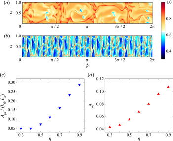
We also investigate the effects of radius ratio on the heat transport from the perspective of plumes. Employing the method introduced in Huang et al. (Reference Huang, Kaczorowski, Ni and Xia2013), van der Poel et al. (Reference van der Poel, Verzicco, Grossmann and Lohse2015b), Chong et al. (Reference Chong, Yang, Huang, Zhong, Stevens, Verzicco, Lohse and Xia2017) and Jiang et al. (Reference Jiang, Zhu, Mathai, Verzicco, Lohse and Sun2018), the cold plume coverage at the edge of the thermal BL of the outer cylinder is obtained. Figure 10(a,b) displays the temperature field near the outer surface for  $\eta = 0.4$ and 0.9, respectively. It is evident that when
 $\eta = 0.9$, the area of cold plumes is larger. Figure 10(c) shows the ensemble-averaged portion of area
 ${A_{pl}}/({L_\phi }{L_z})$ covered by the cold plumes in the vicinity of the outer surface. As
 $\eta$ decreases, a smaller portion of cold plumes can travel to the opposing BL. Consequently, temperature fluctuations of the thermal BL of the outer surface are smaller (see figure 10d) and the heat transfer efficiency declines.
(a) Instantaneous temperature fields in  $\phi z$-plane at the edge of the thermal BL (
 ${r_\delta } = {R_o} - {\delta _T}$) for (a)
 $\eta = 0.4$, (b) 0.9 at
 $Ra = {10^7}$, where
 $\delta _T$ is the thickness of thermal BL obtained using the slope method (Gastine, Wicht & Aurnou Reference Gastine, Wicht and Aurnou2015). To visualize the plumes clearly, the temperature colourbar is from 0.3 to 1. Panels (a,b) share the same colourbar. (c) Ensemble-averaged area of cold plumes normalized by the total area versus
 $\eta$. (d) Ensemble-averaged standard deviation of temperature at the position of
 ${r_\delta }$ versus
 $\eta$.

3.3. Asymmetric mean temperature fields
In classical RBC, due to the Oberbeck–Boussinesq (OB) approximation (Oberbeck Reference Oberbeck1879), it is generally assumed that the fluid properties are constant, except for the linear variation of the density with temperature in the buoyancy term. However, when the temperature difference  $\varDelta$ between the hot and cold walls is large enough, the drastic changing of fluid properties should be taken into consideration. In this situation, the top–bottom symmetry of the system is broken and the bulk temperature
 ${\theta _c}$ deviates from the arithmetic mean temperature of hot and cold walls
 ${\theta _m}$, which are known as non-OB (known as NOB) effects (Wu & Libchaber Reference Wu and Libchaber1991; Yik, Valori & Weiss Reference Yik, Valori and Weiss2020).
Although we implement OB approximation in the numerical simulations of ACRBC, remarkable deviation of  ${\theta _c}$ from
 ${\theta _m}$ is observed, which is similar to the non-OB effects. Figure 11(a) shows the radial temperature profiles averaged azimuthally, axially and over time. It is evident that
 ${\theta _c}$ is much larger than
 ${\theta _m}$. With
 $\eta$ increasing, the deviation
 $({\theta _c} - {\theta _m})/\varDelta$ decreases for each
 $Ra$ (see figure 11b), which illustrates that the mean temperature profile gradually behaves similarly to the classical RBC. We also perform some experiments in the ACRBC system. Details about the experimental set-up are introduced in Jiang et al. (Reference Jiang, Zhu, Wang, Huisman and Sun2020). A small thermistor (Measurement Specialties, GAG22K7MCD419, with a response time of 30 ms in liquids) is inserted into the bulk flow to measure
 ${\theta _c}$. Another type of thermistor (Omega, 44 131), evenly distributed along the circumferential direction in the cylinders, are used to obtain
 ${\theta _m}$. Now
 $({\theta _c} - {\theta _m})/\varDelta$ at
 $\eta = 0.5$ for experiments are slightly larger than the cases of DNS, which probably results from the relatively large
 $Ra$ and
 $Ro^{ - 1}$ for experiments (
 $Ra = 6 \times {10^{10}}$,
 ${Pr} = 4.3$ and
 $Ro^{ - 1} = 18$).
(a) Azimuthally, axially and time-averaged radial temperature profiles for different  $\eta$ at
 $Ra = {10^7}$. (b) Relative deviation of the bulk temperature (
 ${\theta _c}$) from arithmetic mean temperature (
 ${\theta _m}$) of the two cylinders
 $({\theta _c} - {\theta _m})/\varDelta$ versus
 $\eta$ for different
 $Ra$ from DNS (the solid symbols), experiments (the open symbols) and the theoretical prediction given in (3.6) (dashed line). The experiments are performed at
 $\eta = 0.5$,
 $Ra = 6 \times {10^{10}}$,
 ${Pr} = 4.3$ and
 $Ro^{ - 1} = 18$. The solid line denotes
 $({\theta _c} - {\theta _m})/\varDelta$ in pure thermal conduction state for comparison. (c) Ratio of BL temperature scales
 ${\theta ^i}/{\theta ^o}$ versus
 $\eta$ for different
 $Ra$. The horizontal dashed line corresponds to the hypothetical identity
 ${\theta ^i} = {\theta ^o}$ (see (3.5)). (d) Ratio of thermal BL thicknesses. The dashed line corresponds to the theoretical prediction given in (3.8). The inset of panel (d) shows the inner thermal BLs
 ${\lambda ^i}$ highlighted by the blue shaded area.
 ${\lambda ^{i,o}}$ are defined as the distances where the tangents of the temperature profiles at the plate cross
 ${\langle \theta \rangle _{\phi,z,t}} = {\theta _c}$.

Next, we provide a theoretical explanation for the increase of the deviation  $({\theta _c} - {\theta _m})/\varDelta$ with
 $\eta$ decreasing. Since the area of the outer cylinder is larger than that of the inner cylinder, according to Fourier's law, the temperature gradient near the outer wall is smaller. Therefore, the temperature at the midradius position for pure thermal conduction state
 ${({\theta _c})_{cond}} = - ({1}/{{\ln \eta }})\ln [1/2 + 1/(2\eta )]$ (derived in Appendix B) is slightly higher than
 ${\theta _m}=0.5$. Also
 ${({\theta _c})_{cond}} - {\theta _m}$ as a function of
 $\eta$ is indicated by the solid line in figure 11(b). While the curvature effect of ACRBC accounts for a part of
 $({\theta _c} - {\theta _m})/\varDelta$, the difference from the total deviation is still finite. To analytically access
 $({\theta _c} - {\theta _m})/\varDelta$ observed in DNS and experiments, we first assume that heat is purely transported by conduction in the thin thermal BLs. According to the conservation of heat flux through cylindrical surfaces,
 \begin{equation} \eta \frac{{\varDelta {\theta^i}}}{{{\lambda^i}}} = \frac{{\varDelta {\theta^o}}}{{{\lambda^o}}}, \end{equation}
where the thermal BL near the inner (outer) wall is assumed to be a conduction profile with a temperature difference  $\varDelta {\theta ^i}$ (
 $\varDelta {\theta ^o}$) over a thickness
 ${{\lambda ^i}}$ (
 ${{\lambda ^o}}$). Note that different curvatures of the two cylinders are considered in this assumption. As shown in figure 11(a), the bulk fluid is basically isothermal (for small
 $\eta$, the slight overshoot of temperature near the outer surface may result from the effect of Coriolis effects). Thus, we can further assume that the temperature drops occur only in the BLs:
 \begin{equation} \varDelta {\theta^i} + \varDelta {\theta^o} = 1. \end{equation}
Equations (3.3) and (3.4) are not sufficient to determine the three unknowns  $\varDelta {\theta ^i}$,
 $\varDelta {\theta ^o}$ and
 ${\lambda ^i}/{\lambda ^o}$. So an additional physical assumption is required.
Wu & Libchaber (Reference Wu and Libchaber1991), Zhang, Childress & Libchaber (Reference Zhang, Childress and Libchaber1997) and Gastine et al. (Reference Gastine, Wicht and Aurnou2015) proposed that the thermal BLs adjust their length scales so that the mean hot and cold temperature fluctuations are equal in the bulk region. Temperature fluctuations in the bulk region are caused by plumes detaching from the BLs. So this implies the equality of the temperature scales for the two BLs ( ${\theta ^{i,o}} \equiv (\nu \kappa )/(\alpha {g_{i,o}}{({\lambda ^{i,o}})^3})$). This third assumption yields
 \begin{equation} {\theta^i} = {\theta^o} \to \frac{{\nu \kappa }}{{\alpha {g_i}{{({\lambda^i})}^3}}} = \frac{{\nu \kappa }}{{\alpha {g_o}{{({\lambda^o})}^3}}}, \end{equation}
where the centrifugal acceleration  $g = {\omega ^2}r$, so
 ${\chi _g} = g({R_i})/g({R_o}) = {\eta }$ reflects radially dependent gravity effects. Figure 11(c) shows
 ${\theta ^i}/{\theta ^o}$ for different
 $\eta$ and
 $Ra$. Compared with turbulent RB convection in spherical shells reported by Gastine et al. (Reference Gastine, Wicht and Aurnou2015) (see their figure 5a), the identity of the BL temperature scale is better fulfilled in ACRBC. The temperature drops at both boundaries and the ratio of the thermal BL thicknesses can then be derived using (3.3)–(3.5) as
 $$\begin{gather} \varDelta {\theta^i} \simeq {\theta_c} = \frac{1}{{1 + {\chi_g}^{1/3}\eta }} = \frac{1}{{1 +{\eta^{4/3}}}}, \end{gather}$$
 $$\begin{gather}\varDelta {\theta^o} = \frac{1}{{1 + {\eta^{ - 4/3}}}}, \end{gather}$$
 $$\begin{gather}{\lambda^o}/{\lambda^i} = {\eta^{1/3}}. \end{gather}$$
Figure 11(b) shows that the predicted value (3.6) and the actual values for mean bulk temperature are in good agreement. We adopt the slope method to define the thickness of thermal BL  $\lambda$ as the distance where the tangent of the temperature profiles at the plate intersects
 ${\langle \theta \rangle _{\phi,z,t}} = {\theta _c}$ (see the inset of figure 11d). Figure 11(d) shows that the theory (3.8) can also predict the asymmetry of the thermal BLs
 ${\lambda ^o}/{\lambda ^i}$. In a word, the theory accurately accounts for the bulk temperature and the BL asymmetry for different
 $\eta$ observed in ACRBC. The asymmetry is likely caused by the curvature effects (3.3) and radially dependent centrifugal force (3.5). We note that, although asymmetric mean temperature fields exist in ACRBC, their influence on global heat transport has been shown to be negligible (Jiang et al. Reference Jiang, Zhu, Wang, Huisman and Sun2020).
4. Conclusion
We present an analysis of the zonal flow, heat transport and asymmetric mean temperature field in ACRBC, by means of 3-D DNS and some experiments, with radius ratio  $\eta$ varying from 0.3 to 0.9,
 $Ra$ varying from
 ${10^6}$ to
 ${10^8}$ and
 $Pr$,
 $Ro^{ - 1}$ fixed at 4.3 and 1, respectively. Major findings are summarized as follows.
Firstly, convection rolls move anticlockwise around the axis with a faster rotation rate than the background rotation of ACRBC system (zonal flow). We provide two mechanisms for the generation of zonal flow. (1) As the flow is in the inertial regime, the plumes deflect with a radius of curvature  $\widehat R = U/(2\omega )$. The ejection velocity of the cold plumes is larger than that of hot plumes. Thus, the local curvature of the cold plume path is smaller and zonal flow is prograde pushed by the large deflection of hot plumes. (2) Due to the different curvatures of the inner and outer cylinders, the hot plumes can directly affect the ejecting position of the cold plumes, while the impact of the cold plumes does not directly affect the hot plumes. The asymmetric motions of cold and hot plumes push the overall flow to move in the same direction as the background rotation. The mechanism of zonal flow is verified by the variation of the flow behaviour with radius ratio. We observe that the drift frequency decreases with
 $\eta$ increasing. It is also found that
 ${\langle {{u_\phi }} \rangle _{V,t}}$ decreases as
 $\eta$ increases for each
 $Ra$. In addition, zonal flow is the strongest at moderate
 $Ra$ (
 $Ra = {10^7}$), which suggests zonal flow is related to the buoyancy and flow strength.
Secondly, the scaling exponent  $\gamma$ of
 $Nu(Ra)$ increases with
 $\eta$ for
 $\eta \lesssim 0.7$ and slightly decreases for larger
 $\eta$. The dependence of transport efficiency on
 $\eta$ is similar to TC flow. Furthermore,
 $Nu/Nu_{\eta = 0.9}$ decreases with the decrease of
 $\eta$ for each
 $Ra$. By analysing the flow field and the ratio of buoyancy and shear effects, it is found that the flow is in the buoyancy dominated regime and the influence of shear effects of zonal flow on heat transfer is not strong in the parameter space of the current study. Additionally, we observed that the cold plume coverage at the edge of the thermal BL of the outer cylinder becomes smaller as
 $\eta$ decreases.
Thirdly, the bulk temperature  ${\theta _c}$ is found to be much higher than
 ${\theta _m}$ (0.5) by DNS and experiments. The relative deviation
 $({\theta _c} - {\theta _m})/\varDelta$ increases with the decrease of
 $\eta$ for each
 $Ra$. The results of numerical simulations and experiments are consistent, even though the values of
 $Ra$ and
 $Ro^{ - 1}$ are distinct. By assuming pure conduction in the thermal BLs, isothermal bulk fluid, and the equality of the temperature scales for the two boundary layers, we analytically obtain the mean bulk temperature and the ratio of the thickness of the BLs, which are in good agreement with the actual values. The asymmetric mean temperature fields may result from curvature effects and the radially dependent centrifugal force involved in the hypotheses of the theory.
In the laboratory experiment, centrifugal buoyancy can be larger than the Earth's gravity through the rapid rotation of ACRBC. Hypergravitational thermal convection is a new method to achieve high  $Ra$ (Jiang et al. Reference Jiang, Zhu, Wang, Huisman and Sun2020). Systematic study on the dependence of turbulent flow structures and heat transport on radius ratio is urgently needed to understand the flow dynamics in ACRBC. The physical mechanism of zonal flow may improve understanding of some flow phenomena in astrophysical and geophysical settings. Furthermore, the bulk temperature can be significantly increased in the hypergravitational thermal convection system by reducing
 $\eta$, which give insights for the flow and temperature control in engineering applications.
Supplementary movies
Supplementary movies are available at https://doi.org/10.1017/jfm.2021.889.
Funding
This work was supported by the Natural Science Foundation of China (grant nos. 11988102, 91852202, 11861131005) and Tsinghua University Initiative Scientific Research Program (grant no. 20193080058).
Declaration of interests
The authors report no conflict of interest.
Appendix A. Derivation of the governing equations
Below we provide the detailed derivation of the non-dimensional governing equations. Firstly, for ACRBC the fluid motion in the rotating reference frame is governed by the continuity equation, the thermal advection–diffusion equation and the Navier–Stokes equation with centrifugal force and Coriolis force, which read
 $$\begin{gather} \boldsymbol{\nabla}\boldsymbol{\cdot} \boldsymbol{u} = 0, \end{gather}$$
 $$\begin{gather}\frac{{\partial T}}{{\partial t}} + (\boldsymbol{u} \boldsymbol{\cdot} \boldsymbol{\nabla})T = \kappa{\nabla^2}T, \end{gather}$$
 $$\begin{gather}\frac{{\partial \boldsymbol{u} }}{{\partial t}} + (\boldsymbol{u} \boldsymbol{\cdot} \boldsymbol{\nabla})\boldsymbol{u} ={-} \frac{1}{\rho }\boldsymbol{\nabla} p - 2\boldsymbol{\omega} \times \boldsymbol{u} + \nu {\nabla^2}\boldsymbol{u} - \boldsymbol{\omega} \times (\boldsymbol{\omega} \times \boldsymbol{r}). \end{gather}$$
Here  $\boldsymbol {u}$,
 $t$,
 $T$ and
 $p$ are the velocity, time, temperature and pressure of the flow;
 $\rho$,
 $\nu$,
 $\kappa$ are the density, kinematic viscosity, thermal diffusivity of the working fluid, respectively;
 $\boldsymbol {\omega }$ is the angular velocity of the system. Different from Navier–Stokes equation in the inertial frame, two additional terms appear and they are the Coriolis force
 $- 2\boldsymbol {\omega } \times \boldsymbol {u}$ and the centrifugal force
 $- \boldsymbol {\omega } \times (\boldsymbol {\omega } \times \boldsymbol {r})$.
Secondly, spatially and temporally constant temperatures are assumed at the hot and cold surfaces. The problem is simplified by the OB approximation in which the fluid density  $\rho$ is assumed to depend linearly on the temperature only in the centrifugal buoyancy term,
 \begin{equation} \rho (T) = \rho ({T_0})[1 - \alpha (T - {T_0})], \end{equation}
where  ${T_0}$ is the reference temperature at the inner cylinder. Here
 $\alpha$ is the thermal expansion coefficient of the working fluid. Substituting (A4) into (A3), the governing equations are
 $$\begin{gather} \boldsymbol{\nabla}\boldsymbol{\cdot} \boldsymbol{u} = 0, \end{gather}$$
 $$\begin{gather}\frac{{\partial T}}{{\partial t}} + (\boldsymbol{u} \boldsymbol{\cdot}\boldsymbol{\nabla})T = \kappa{\nabla^2}T, \end{gather}$$
 $$\begin{gather}\frac{{\partial \boldsymbol{u}}}{{\partial t}} + (\boldsymbol{u} \boldsymbol{\cdot} {\boldsymbol{\nabla}})\boldsymbol{u} ={-} \frac{1}{\rho }\boldsymbol{\nabla} p - 2 \boldsymbol{\omega} \times \boldsymbol{u} + \nu {{\nabla}^2}\boldsymbol{u} - \alpha \delta T {\omega^2}\boldsymbol{r}. \end{gather}$$
Here,  $\delta T = T - {T_0}$ is the temperature difference from the reference temperature.
Thirdly, we non-dimensionalize the set of equations using the gap width L, the free-fall velocity  $U \equiv \sqrt {{\omega ^2}({{({R_o} + {R_i})}}/{2})\alpha \varDelta L}$ (
 ${R_o}$ and
 ${R_i}$ are the radius of the outer and inner cylinders, respectively) and the temperature difference of the inner and outer cylinders
 $\varDelta$. Then we arrive at the dimensionless governing equations as follows:
 $$\begin{gather} \widetilde{\boldsymbol{\nabla}} \boldsymbol{\cdot} \widetilde {\boldsymbol{u} } = 0, \end{gather}$$
 $$\begin{gather}\frac{{\partial \widetilde \theta }}{{\partial \widetilde t}} + \widetilde {\boldsymbol{{u}} } \boldsymbol{\cdot} \widetilde {\boldsymbol{\nabla}}\widetilde \theta = \frac{\kappa }{{\omega L\sqrt {({R_o} + {R_i})\alpha \varDelta L/2}}}{\widetilde{\nabla}^2}\widetilde \theta, \end{gather}$$
 \begin{gather} \frac{{\partial \widetilde {\boldsymbol{u} }}}{{\partial \widetilde t}} + \widetilde {\boldsymbol{u} } \boldsymbol{\cdot} \widetilde {\boldsymbol{\nabla}}\widetilde {\boldsymbol{u} } ={-} \widetilde {\boldsymbol{\nabla}}\widetilde p - 2\left (\frac{{\alpha \varDelta ({R_o} + {R_i})}}{{2L}}\right )^{ - 1/2} \widehat {\boldsymbol{\omega} } \times \widetilde{\boldsymbol{u} } \nonumber\\ \hspace{-1pc}+ \frac{\nu }{{\omega L\sqrt {({R_o} + {R_i})\alpha \varDelta L/2}}}{\widetilde{\nabla}^2} \widetilde {\boldsymbol{u} } -\widetilde \theta \frac{{2L}}{{{R_i} + {R_o}}} \widetilde {\boldsymbol{r} }, \end{gather}
where  $\widetilde r = r/L$ and
 $\widetilde t = tU/L$ are the scaled space and time coordinates;
 $\widetilde {\boldsymbol {u} } = \boldsymbol {u} /U$,
 $\widetilde p = (p - \rho ({T_0}){\omega ^2}R_i^2/2)/(\rho ({T_0}){U^2})$;
 $\widetilde \theta = (T - {T_0})/\varDelta$ are the scaled velocity, the scaled pressure and temperature variation, respectively;
 $\widehat {\boldsymbol {\omega }}$ is the unit vector pointing in the direction of the angular velocity.
Lastly, four dimensionless parameters will be deduced in the governing equations:
 $$\begin{gather} \eta = {R_i}/{R_o}, \end{gather}$$
 $$\begin{gather}Ra = \tfrac{1}{2}{\omega^2}({R_o} + {R_i})\alpha \varDelta {L^3}/(\nu\kappa), \end{gather}$$
 $$\begin{gather}{Pr} = \nu /\kappa, \end{gather}$$
 $$\begin{gather}Ro^{ - 1} = 2\omega L/U = 2{(\alpha \varDelta ({R_o} + {R_i})/(2L))^{-({1}/{2})}}. \end{gather}$$
Substituting these control parameters (A11)–(A14) into (A8)–(A10), we obtain
 $$\begin{gather} \widetilde{\boldsymbol{\nabla}}\boldsymbol{\cdot}\widetilde {\boldsymbol{u} } = 0, \end{gather}$$
 $$\begin{gather}\frac{{\partial \widetilde \theta }}{{\partial \widetilde t}} + \widetilde {\boldsymbol{{u}} } \boldsymbol{\cdot} \widetilde {\boldsymbol{\nabla}}\widetilde \theta = \frac{1}{{\sqrt{RaPr} }}{\widetilde {\nabla}^2}\widetilde \theta, \end{gather}$$
 $$\begin{gather}\frac{{\partial \widetilde {\boldsymbol{u}}}}{{\partial \widetilde t}} + \widetilde {\boldsymbol{{u}} } \boldsymbol{\cdot} \widetilde {\boldsymbol{\nabla}}\widetilde {\boldsymbol{{u}} } ={-} \widetilde {\boldsymbol{\nabla}}\widetilde p - Ro^{- 1}\widehat {\boldsymbol{\omega} } \times \widetilde {\boldsymbol{{u}} } + \sqrt {\frac{{Pr}}{{Ra}}}{\widetilde{\nabla}^2}\widetilde {\boldsymbol{{u}} } - \widetilde \theta \frac{{2(1 -\eta )}}{{(1 + \eta )}}\widetilde {\boldsymbol{{r}}}. \end{gather}$$
For clarity, the wave line cap  $\widetilde \bullet$ for the dimensionless quantity is omitted. The resulting equations correspond to the (2.1)–(2.3).
Appendix B. Derivation of  $Nu$ in ACRBC

Due to the cylindrical geometry of the convection system, the definition of  $Nu$ in ACRBC is slightly different from that in the classical RBC. Here we derive the expressions (2.5) of
 $Nu$. When there is only pure conduction between the hot and cold cylinders, the energy equation reads
 \begin{equation} \frac{\textrm{d}}{\textrm{d}r}\left(r\frac{\textrm{d}\theta}{\textrm{d}r}\right)=0, \end{equation}
and the boundary conditions,  $\theta (R_i)=\theta _{cold}$,
 $\theta ({R_o})=\theta _{hot}$, so we have the temperature profile along radial direction as
 \begin{equation} \theta=\theta_{cold}+(\theta_{hot}-\theta_{cold})\frac{\ln(r/R_i)}{\ln(R_o/R_i)}, \end{equation}
and consequently the heat flux by pure conduction,
 \begin{equation} J_{con}={-}\chi \frac{\textrm{d}\theta}{\textrm{d}r}=\frac{\chi \varDelta}{r \cdot \ln(\eta)}, \end{equation}
where  $\chi =\kappa \rho c_p$ is the thermal conductivity of the working fluid with
 $\rho$ and
 $c_p$ the density and the specific heat capacity of the fluid,
 $\varDelta =\theta _{hot}-\theta _{cold}$ the temperature difference between the hot and cold cylinders and
 $\eta =R_i/R_o$. Besides, the temperature at the midradius position
 ${R_i} + ({R_o} - {R_i})/2$ for pure thermal conduction state is
 \begin{equation} {({\theta_c})_{cond}} ={-} \frac{1}{{\ln \eta }}\ln [1/2 + 1/(2\eta )]. \end{equation}
The thermal convection–diffusion equation reads
 \begin{equation} \frac{\partial \theta}{\partial t} +\boldsymbol{u}\boldsymbol{\cdot}\boldsymbol{\nabla} \theta=\kappa\nabla^2 \theta, \end{equation}
and in cylindrical coordinates it reads
 \begin{align} \frac{\partial \theta}{\partial t} +\frac{1}{r}\frac{\partial}{\partial r}\left(r\left(u_r\theta-\kappa\frac{\partial \theta}{\partial r}\right)\right)+\frac{1}{r}\frac{\partial }{\partial \varphi}\left(u_{\varphi}\theta-\frac{\kappa}{r}\frac{\partial \theta}{\partial \varphi}\right)+\frac{\partial}{\partial z}\left(u_z\theta-\kappa \frac{\partial \theta}{\partial z}\right)=0. \end{align}
Averaging this equation azimuthally, axially and temporally, we obtain
 \begin{equation} \frac{1}{r}\frac{\partial}{\partial r}\left(r\left(\langle u_r\theta\rangle_{t,\varphi,z}-\kappa\frac{\partial }{\partial r}\langle \theta\rangle_{t,\varphi,z}\right)\right)=0, \end{equation}
meaning
 \begin{equation} r\left(\langle u_r\theta\rangle_{t,\varphi,z}-\kappa\frac{\partial }{\partial r}\langle \theta\rangle_{t,\varphi,z}\right)=\text{constant}. \end{equation}
Hence the convective heat flux can be expressed as
 \begin{equation} J=\rho c_p\left(\langle u_r\theta\rangle_{t,\varphi,z}-\kappa\frac{\partial }{\partial r}\langle \theta\rangle_{t,\varphi,z}\right). \end{equation}
Finally, using (B3) and (B9), we can define the  $Nu$ as
 \begin{equation} Nu=\frac{J}{J_{con}}=\frac{\langle u_r\theta\rangle_{t,\varphi,z}-\kappa\dfrac{\partial }{\partial r}\langle \theta\rangle_{t,\varphi,z}}{\kappa \varDelta (r\cdot \ln(\eta) )^{{-}1}}. \end{equation}
The columns from left to right indicate the following: radius ratio  $\eta$, Rayleigh number Ra, the maximum grid spacing
 ${\varDelta _g}$ compared with the Kolmogorov scale estimated by the global criterion
 ${\eta _K} = {{L{{Pr }^{1/2}}}}/{{[{Ra(Nu - 1)}]}^{1/4}} \cdot {[{{(1 + \eta )\ln (\eta )}}/{{2(\eta - 1)}}]^{1/4}}$ (Jiang et al. Reference Jiang, Zhu, Wang, Huisman and Sun2020), the number of grid points within the thermal BL
 ${N_{tBL}}$ and viscous BL
 ${N_{vBL}}$, the averaging time period
 ${\tau _{avg}}$, Nusselt number
 $Nu$, the difference of
 $Nu$ between inner and outer walls
 ${\epsilon _{Nu}} = | Nu_{{in}} - Nu_{{out}} |/Nu$, aspect ratio
 $\varGamma$, reduced azimuthal domain
 ${\phi _0}$, the resolution in azimuthal, axial, and radial directions
 ${N_\phi } \times {N_z} \times {N_r}$. Note that the azimuthal resolution corresponds to the resolution of the segment. For example,
 ${N_\phi } = 1024$ for
 ${\phi _0} = 1/2$ means 1024 points for one half of the annulus