





1. Introduction
In Rismondo et al. (Reference Rismondo, Petris, Cianferra and Armenio2025) (hereafter RPCA25), the authors studied the problem of fluid-dynamic noise generated by a model-scale rotor of a wind turbine. In the Conclusions, the authors highlighted the need to extend the study considering the actual configuration of a complete wind turbine, comprehensive of the mast, the nacelle and the presence of the ground, which may act as a reflecting surface for the acoustic waves. This is the topic of the present paper, which represents the natural extension of RPCA25 and focuses on the fluid-dynamic noise generated by a complete, model-scale wind turbine.
The study is justified by the rapid growth of the wind turbine energy sector in the last few years (see Council (2025) for a detailed discussion); this growth poses significant challenges for industries and researchers in minimizing the negative impact of wind energy on the natural and built environment (Veers et al. Reference Veers2023). Among others, noise pollution constitutes a serious issue for wildlife species and human beings.
The isolated rotor (IR) produces a complex fluid-dynamic field, composed of a three-dimensional boundary layer over the blades, a vortex sheet behind the blades and a three-region wake (see RPCA25 and the literature therein reported). The fluid-dynamic field over the blades induces intense pressure fluctuations, promoting noise generation, especially from the blade trailing edge; noise exhibits both a tonal character at the blade passing frequency (BPF) and a broadband character in the range of high frequencies. The fluid-dynamic noise associated with the wake plays a significant role in the low-frequency range in the very near field, especially along the wake direction. The tip vortex instability, which promotes wake destabilization, is responsible for the transition from a tonal to a broadband character of the nonlinear acoustic footprint.
As discussed in RPCA25, most of the literature focuses on the fluid dynamics and acoustics of the IR; comparatively few studies have been devoted to the analysis of the complete wind turbine, composed of the rotor, the nacelle and the tower. The fluid-dynamic interaction between the three elements makes the flow field substantially different from that developing around the IR and may have a significant impact on the fluid-dynamic noise produced by the complete wind turbine. In addition, the presence of the ground generates a boundary layer and acts as a reflective surface for acoustic waves, playing a role in the propagation of sound.
Specifically, the tower affects tip vortex breakdown and momentum recovery, giving rise to a phenomenon known in the literature as blade–tower interaction (BTI), with subsequent noise generation. The BTI is present in a wide class of rotor–structure interaction processes and plays a significant role across various engineering domains; it influences the acoustic and fluid-dynamic performance of systems, spanning from rotor–rudder configurations in naval hydrodynamics (see for example Posa et al. (Reference Posa, Broglia and Felli2024)) to rotor–pylon and rotor–tail boom configurations in aeronautics aerodynamics (Leishman & Bi Reference Leishman and Bi1990; Enoki et al. Reference Enoki, Kodama and Kusuda2013).
The literature studies (see, among others, Porté-Agel et al. (Reference Porté-Agel, Bastankhah and Shamsoddin2020)) show that in the case of a complete wind turbine, BTI makes the fluid-dynamic field substantially different from that developing in the case of an IR. A near wake is present, roughly extending by
 $1{-}4$
rotor diameters
 $D$
, characterized by coherent vortical structures, such as tip and root vortices, the blade wake and the tower’s vortex shedding; beyond that, a fully turbulent composite far wake develops, which exhibits a slow oscillatory behaviour, known as wake meandering.
The turbulent inflow, the tip speed ratio (
 $\textit{TSR} = \varOmega R/U_{\infty }$
, where
 $U_\infty$
is the upstream undisturbed velocity,
 $R$
is the radius of the rotor and
 $\varOmega$
is its rotation rate), and the presence of the tower and nacelle are known to promote a faster wake destabilization relative to the IR, with consequent rapid momentum recovery; such aspects have been widely studied using both physical and numerical experiments considering the full wind turbine.
The effect of the tower has been the subject of analysis in the wind tunnel experiment of Pierella & Sætran (Reference Pierella and Sætran2017); the study showed that the presence of the tower generates an asymmetry in the wake, thereby promoting a net imbalance in vertical momentum transport. Consequently, the mean wake structure has been observed to shift below the rotor axis and to grow in the horizontal direction more than in the vertical one. Abraham et al. (Reference Abraham, Dasari and Hong2019) conducted a wind tunnel experiment for an operational
 $2.5$
MW wind turbine and analysed the influence of the tower and the nacelle on the mechanisms involved in the evolution of the wake.
The influence of free stream turbulence on a complete model-scale wind turbine was addressed experimentally by Gambuzza & Ganapathisubramani (Reference Gambuzza and Ganapathisubramani2023) (hereafter GG23); the study showed that an increased turbulence intensity level in the inflow results in a faster wake destabilization and faster wake recovery. The effect of tip speed ratio on the near wake was investigated in the experiments of Biswas & Buxton (Reference Biswas and Buxton2024a) for a model-scale wind turbine. They proposed a novel definition of the near wake and far wake, based on the strength of the tip vortex system, characterizing the near wake, and the process of wake meandering, associated with the far wake. Furthermore, the authors emphasized that BTI enhances the destabilization of the tip vortex, thereby promoting turbulent mixing. In subsequent work, Biswas & Buxton (Reference Biswas and Buxton2024b) performed optimal mode decomposition to investigate energy exchange between coherent structures in the near wake, considering different tip-speed ratios. The authors found that the tip vortex system generates a complex nonlinear triadic energy exchange between coherent modes associated with the revolution frequency
 $f_T$
and its superharmonics.
Recently, in Bourhis et al. (Reference Bourhis, Messmer, Hölling and Buxton2025), the authors investigated the effects of free stream turbulence and thrust coefficient, representative of typical operating conditions, on the wind turbine wake; challenging the conventional wake definitions established for non-turbulent inflows, they make it evident that the wake dynamics of wind turbines share common features with those of simplified surrogates, such as porous disks, the analysis indicates that similar flow mechanisms govern both bluff-body and turbine wakes.
From a mathematical modelling perspective, the combination of the actuator technique (Sorensen & Shen Reference Sorensen and Shen2002; Mikkelsen Reference Mikkelsen2004) with the immersed boundary technique (Peskin Reference Peskin2002) has been widely used to model the rotor and the tower/nacelle, respectively. In this approach, the fluid-dynamics processes in the complete wind turbine wake are obtained by numerical solution of the Navier–Stokes equations, coupled with the actuator technique–immersed boundary methods to model the complete machine. Among others, Kang et al. (Reference Kang, Yang and Sotiropoulos2014) performed large-eddy simulations (LES) of a hydrokinetic turbine, mimicking the experiment of Chamorro et al. (Reference Chamorro, Hill, Morton, Ellis, Arndt and Sotiropoulos2013), using immersed boundary, actuator line and actuator disk modelling. The study revealed that instability of root vortices initiates a meandering motion within the near wake, which, upon reaching the surrounding annular shear layer, accelerates its disruption and drives the onset of the far-wake transition. Further, the authors noted that models lacking geometric detail, such as the actuator disk model, fail to capture some of the above-mentioned effects, highlighting the potential of near-hub rotor design improvement to suppress root vortex instability and reduce far-wake meandering. Wind turbine wake stability is addressed by Sarmast et al. (Reference Sarmast, Dadfar, Mikkelsen, Schlatter, Ivanell, Sørensen and Henningson2014), analysing the results of a LES paired with the actuator line model, using the dynamic mode decomposition and proper orthogonal decomposition (POD), highlighting that the main unstable modes are associated with the process of mutual inductance mode between successive tip vortices. Debnath et al. (Reference Debnath, Santoni, Leonardi and Iungo2017), the authors applied different dynamic reduced-order models to two LES datasets, in which the wind turbine, immersed in an atmospheric boundary layer, was modelled using the actuator line technique with and without the tower and nacelle. It was emphasized that, for the IR, the processes of wake destabilization and wake recovery are primarily governed by the instability of the tip vortex system and its downward transport. Conversely, in the presence of BTI, the nonlinear interaction between the tip vortex system and the tower’s vortex shedding promotes faster wake destabilization. Santoni et al. (Reference Santoni, Carrasquillo, Arenas-Navarro and Leonardi2017) performed simulations with and without the tower and nacelle to investigate their effect on wake development, considering two different tip speed ratios. Beyond causing a velocity deficit, the tower and nacelle also alter the distribution of turbulent kinetic energy (TKE) and its downward transport. Their wake merges with that of the blades, facilitating the destabilization of tip vortices and amplifying the kinetic energy transfer into the wake region. De Cillis et al. (Reference De Cillis, Cherubini, Semeraro, Leonardi and De Palma2021) used POD, considering two configurations, with and without the presence of the tower and nacelle, respectively. In addition, in De Cillis et al. (Reference De Cillis, Semeraro, Leonardi, De Palma and Cherubini2022), the authors extended their previous work by evaluating the dynamic mode decomposition of the wake generated by the NREL 5 MW wind turbine (National Renewable Energy Laboratory) (modelled with LES and immersed boundary technique) and identifying the most coherent dynamic structures characterizing the wake. The authors showed that the tower and the nacelle introduce low-frequency POD modes in the near wake, associated with von Kármán vortex shedding generated by the tower. Downstream, these modes interact nonlinearly with tip vortices, generating additional low-frequency modes. This interaction accounts for the accelerated momentum recovery observed in the presence of the tower and nacelle.
Other numerical studies are based on geometry-resolving simulations using the sliding mesh method or overset grid method to take into account the rotor together with the tower, adopting the Reynolds-averaged Navier–Stokes equations or delayed detached eddy simulation. In Zahle et al. (Reference Zahle, Sørensen and Johansen2009), Hsu & Bazilevs (Reference Hsu and Bazilevs2012) and Mo et al. (Reference Mo, Choudhry, Arjomandi and Lee2013), the authors found a periodic variation in the loads acting on the blade and in the power output; these effects were associated with BTI. In fact, the rotor–tower interaction produces periodic load fluctuations on the blades, with rapid deloading and reloading due to the tower wake deficit and the interaction with shed vortices, resulting in a highly unsteady response. The results of Wang et al. (Reference Wang, Zhou and Wan2012) indicate that the tower has a minor impact on the overall aerodynamics of an upwind turbine, although the rotor induces a cyclic pressure drop on the tower front, with strong interactions between blade tip vortices and tower-induced separation. Nelson et al. (Reference Nelson, Cain, Raman, Chan, Saunders, Noble, Engeln, Dougherty, Brentner and Morris2012) performed geometry-resolving delayed detached eddy simulation of the complete machine using the dynamic mesh method to predict the near-field, therefore accounting for BTI.
The periodic variations of the pressure acting on the blade and the tower promoted by BTI affect noise generation mechanisms (see, among the others Curle (Reference Curle1955), Yauwenas et al. (Reference Yauwenas, Zajamšek, Reizes, Timchenko and Doolan2017) and Yauwenas et al. (Reference Yauwenas, Zajamšek, Reizes, Timchenko and Doolan2021)). Consequently, noise associated with BTI exhibits a periodic and impulsive character and represents an important source of low-frequency noise which has an impact on underwater noise propagation, in the case of offshore wind farms (see, among others, Yu et al. (Reference Yu, Li, Guo, Qi, Li, Zhu, Wang and Sun2024) and the literature therein reported). These effects define the characteristic tonal peaks at the BPF and its superharmonics, and also modulate other fundamental noise rotor mechanisms. The abrupt variations in flow conditions around the blade, especially upstream of the tower, can influence the so-called trailing-edge noise (Lee et al. Reference Lee, Ayton, Bertagnolio, Moreau, Chong and Joseph2021) through sudden changes in boundary-layer state and wake dynamics. The altered tip-flow structures may further influence the tip vortex noise, whose origin is still not fully understood.
Experimental investigations have significantly contributed to understanding rotor noise generation. In the case of wind turbines, studies have shown that the radiated sound power correlates with rotor rotational speed, or equivalently, with blade-tip speed, better than with the ambient wind speed alone, that changes in blade geometry have only a marginal effect on noise levels, and that trailing-edge noise is the dominant source (see, among others, Debruijn et al. (Reference Debruijn, Stam and Dewolf1984), Van der Borg & Vink (Reference Van der Borg and Vink1994), Oerlemans et al. (Reference Oerlemans, Sijtsma and López2007) and Ramachandran et al. (Reference Ramachandran, Raman and Dougherty2014)).
In a wind tunnel experiment, Yu et al. (Reference Yu, Li, Guo, Qi, Li, Zhu, Wang and Sun2024) examined radiated noise, focusing on the role of flow unsteadiness in the near wake of a wind turbine tower; they found that aerodynamic noise downstream of the tower is associated with enhanced momentum exchange, which leads to an increase in TKE, resulting in velocity and pressure fluctuations, and consequently, noise generation. Recently, in Duc & Finez (Reference Duc and Finez2025), the authors performed experimental measurements, considering a commercial wind turbine, to derive ground-level turbine noise directivity, highlighting the typical dipole shape with a slight asymmetry, which is not accounted for by the analytical model.
For engineering applications, the generation and propagation of rotor noise is often estimated using semiempirical or analytical approaches; for more details, we refer to Zhu et al. (Reference Zhu, Shen, Barlas, Bertagnolio and Sørensen2018), Lee et al. (Reference Lee, Ayton, Bertagnolio, Moreau, Chong and Joseph2021) and the literature therein reported.
The potential flow assumption in conjunction with the theory of Curle (Reference Curle1955) for far-field acoustic pressure evaluation was adopted by Doolan et al. (Reference Doolan, Moreau and Brooks2012) to describe the origin of BTI in wind turbines; their results suggest that tonal acoustic pressure pulsations at the BPF are due to the aerodynamic interaction between the blade and the tower. The blade element momentum theory, paired with the potential flow assumption around the tower, was employed by Madsen (Reference Madsen2010) to model a three-blade rotor with the presence of the tower in both upwind and downwind configurations; they highlighted that the distance between the blade and the tower plays a role in BTI generated noise. Yauwenas et al. (Reference Yauwenas, Zajamšek, Reizes, Timchenko and Doolan2017), Zajamsek et al. (Reference Zajamsek, Yauwenas, Doolan, Hansen, Timchenko, Reizes and Hansen2019) and Yauwenas et al. (Reference Yauwenas, Zajamšek, Reizes, Timchenko and Doolan2021) performed experimental and numerical analyses to study BTI noise-generation from upwind turbines using Reynolds-averaged Navier–Stokes equations over a dynamic grid in conjunction with the acoustic analogy of Curle (Reference Curle1955); their numerical results revealed that the tower is the primary noise source, radiating nearly twice the noise of the blades, and highlighted the need for eddy-resolving simulations, such as LES.
In recent years, computational aeroacoustics and hydroacoustics have become standard tools for predicting rotor noise in a wide range of engineering applications. High-fidelity simulations typically rely on the acoustic analogy (Lighthill Reference Lighthill1952) and its extension to moving bodies through the Ffowcs Williams–Hawkings (FWH) equation (Ffowcs Williams & Hawkings Reference Ffowcs Williams and Hawkings1969), which separates noise into surface-generated (linear) and flow-induced (nonlinear) contributions. Historically, a number of studies have neglected the wake-related (nonlinear) contribution, assuming it to be negligible in the far field and focusing solely on the linear loading and thickness terms (examples are in for example Nelson et al. (Reference Nelson, Cain, Raman, Chan, Saunders, Noble, Engeln, Dougherty, Brentner and Morris2012), Wang et al. (Reference Wang, Wang and Wang2021) and Zhou et al. (Reference Zhou, Wang and Wang2024)). Although these terms often dominate the far-field acoustics, later studies have shown that nonlinear sources from the wake can play a significant role both in the near field and in the intermediate one, particularly in low-Mach flows or in configurations with multiple rotating sources, as underlined by Ianniello (Reference Ianniello2016), and Cianferra & Armenio (Reference Cianferra and Armenio2021). Accurate assessment of these nonlinear contributions requires eddy-resolving simulations and careful treatment of compressibility effects (Wang et al. Reference Wang, Freund and Lele2006; Cianferra et al. Reference Cianferra, Ianniello and Armenio2019a ). Recent investigations on both wind and marine rotors confirm the importance of accounting for both linear and nonlinear terms, often using LES coupled with FWH-based approaches, to capture the complete acoustic signature of rotating machinery (Bensow & Liefvendahl Reference Bensow and Liefvendahl2016; Kimmerl et al. Reference Kimmerl, Mertes and Abdel-Maksoud2021; Stark & Shi Reference Stark and Shi2021; Posa et al. Reference Posa, Broglia and Felli2022a , Reference Posa, Broglia, Felli, Cianferra and Armeniob , Rismondo et al. Reference Rismondo, Petris, Cianferra and Armenio2025; Rismondo et al. Reference Rismondo, Petris, Cianferra and Armenio2025). Despite the number of numerical studies present in the literature devoted to the analysis of the tower/nacelle-influencing fluid-dynamic processes in wind turbine wake (see the literature mentioned above), to the best of our knowledge Nelson et al. (Reference Nelson, Cain, Raman, Chan, Saunders, Noble, Engeln, Dougherty, Brentner and Morris2012) is the only study that adopted a geometry-resolving approach in conjunction with delayed detached eddy simulation, paired with the linear formulation of the FWH equation, to predict the far-field wind turbine noise, considering the complete machine. However, their analysis did not consider the tower as a source of noise and the nonlinear noise component due to the fluid-dynamics processes. To summarize, in the field of wind turbines, the influence of the tower (BTI) on fluid-dynamic and acoustic processes has not been widely investigated considering high-fidelity geometry-resolving simulations, such as LES and computational aeroacoustics. This is not the case in other disciplines, such as naval hydrodynamics and aeronautics, in which the case of a rotor interacting with an upstream or downstream obstacle, for instance, a pylon or a hydrofoil (marine rudder), has been studied considering high-fidelity numerical simulation and acoustic analogy (see, among the others, Wang et al. (Reference Wang, Wang and Wang2021), Posa et al. (Reference Posa, Broglia and Felli2022), Zhou et al. (Reference Zhou, Wang and Wang2024) and Posa et al. (Reference Posa, Broglia and Felli2024)).
In the present paper, we perform the aerodynamic analysis of a model-scale wind turbine considering the presence of both the tower and the nacelle. We also consider the presence of the ground from an acoustics point of view. Specifically, we consider the rotor of the wind turbine analysed in the laboratory experiment of GG23 as well as in the numerical study of RPCA25, at a Reynolds number of
 $96\,000$
, based on the diameter of the wind turbine and the inflow velocity. We perform geometry-resolving simulations in conjunction with wall-resolved LES to reproduce the wind turbine wake evolution up to
 $5D$
, capturing the nonlinear interaction between the tip vortex system and the tower, the tip vortex instability, and wake destabilization.
First, we perform the numerical simulation and analyse the fluid-dynamic field in view of the relevant literature and the results of RPCA25 relative to the case of the IR. The LES of the model-scale wind turbine allows detection of the main features of the wind turbine wake, namely tip and root vortices, the thin trailing edge vortex sheet released by the blade, the tower’s vortex shedding and their time–space evolution from the near to the far wake. This level of accuracy can highlight the instability mechanism that involves the wake of the wind turbine and the role covered by the presence of the tower. Successively, we analyse the acoustic field. Computational aeroacoustics is used here considering two scenarios: the first one where noise propagation is considered in an infinite space, which represents an idealized case; the second one considers the presence of the ground, modelled as a reflecting bottom surface and, thus, noise is propagated into a semi-infinite domain.
The use of such a two-step methodology allows us to better understand the effect of nonlinear interaction between the tip vortex system and the tower on radiated noise, and the mechanism of generation and propagation of sound generated by a wind turbine in a scenario more realistic than the case of the IR.
The paper is structured as follows: § 2 describes the mathematical model, both for the fluid-dynamic field and for the aeroacoustic analysis; § 3 reports the results of the fluid-dynamic field, considering separately the near wake and far wake dynamics; § 4 reports the acoustic analysis, describing first the characteristics of the noise source, and successively the acoustic field in the two cases described above; finally, § 5 contains concluding remarks.
2. Methodology
2.1. Fluid dynamic model
The incompressible flow assumption is the most suitable for wind turbine aerodynamics, justified by the typical value of the rotational Mach number, of the order of
 ${\sim} 0.1$
. In RPCA25 the axial symmetry of the problem allowed the authors to consider the filtered incompressible Navier–Stokes equations in a rotating frame of reference; in the present context, the presence of the tower requires a different approach. We solved the equations in the arbitrary Lagrangian–Eulerian frame of reference (Duarte et al. Reference Duarte, Gormaz and Natesan2004), which enables the region containing the blades to rotate while the rest of the domain containing the tower remains fixed in space. The equation set reads
 \begin{align} \frac {\partial (\overline {u}_i - {v}_i)}{\partial x_i} &= 0, \end{align}
 \begin{align} \frac {\partial \overline {u}_i}{\partial t} + \frac {\partial ((\overline {u}_i-v_i)\, \overline {u}_{\!j})}{\partial x_{\!j}} &= - \frac {\partial \overline p}{\partial x_i} + \nu \frac {\partial ^2 \overline {u}_i}{\partial x_{\!j} \partial x_{\!j}} + \frac {\partial \tau _{\textit{ij}}}{\partial x_{\!j}}, \end{align}
where
 $x_i$
is the spatial coordinate in the
 $i$
-direction,
 $\overline {u}_i$
and
 $\overline {p}$
are the filtered fluid velocity component in the
 $i$
-direction in the fixed frame of reference and kinematic pressure, respectively (for simplicity, they are hereafter denoted as
 $u_i$
and
 $p$
),
 $v_i = (\boldsymbol{\varOmega } \times \boldsymbol {r})_i$
is the mesh velocity component in the rotating region,
 $\boldsymbol {r}$
is the distance of the point in space from the centre of rotation,
 $\boldsymbol{\varOmega } = (\varOmega \; 0 \; 0)$
is the rotating velocity vector and
 $\nu$
is the kinematic viscosity.
The subgrid-scale stress tensor
 $\tau _{\textit{ij}}$
is modelled using the wall-adapting local eddy-viscosity model proposed by Ducros et al. (Reference Ducros, Nicoud and Poinsot1998). The governing equations are solved with the `pressure implicit with splitting of operators’ algorithm, as implemented in the open-source finite-volume framework OpenFOAM (Weller et al. Reference Weller, Tabor, Jasak and Fureby1998), employing an unstructured mesh.
The computational domain is composed of a rotating and a stationary region, which are coupled through the non-conformal coupling method, natively supported in OpenFOAM. Time derivatives are discretized using the backward implicit scheme, which is second-order accurate, while spatial terms are treated with the second-order Gauss integration scheme combined with linear (central differencing) interpolation.
For the solution of the momentum equation, the algorithm employs a biconjugate gradient solver with preconditioning (Van der Vorst Reference Van der Vorst1992). The pressure–velocity coupling is carried out with a predictor–corrector approach, with the Poisson equation solved using the geometric agglomerated algebraic multigrid method. Two predictor–corrector iterations and two non-orthogonal corrections are used per time step, ensuring second-order accuracy in both space and time.
Simulations are carried out with a fixed time step of
 $\varDelta t = 1.0 \times 10^{-6} \text{s}$
, yielding a maximum Courant number
 $Co_{\textit{max}} \sim 10$
for a few localized cells near the blade leading edge, while the average value of Courant number remains around
 $0.017$
. Specifically, these cells are located in the outer region of the boundary layer where tetrahedral transitional cells are employed. It has been verified that, in this region, the local field variables are smooth and physically consistent. Flow statistics are computed over five full rotational periods.
2.2. Acoustic model
Since the seminal work of Lighthill (Reference Lighthill1952), which first established the foundations of aerodynamic sound generation, substantial progress has been made in extending acoustic analogy theory to more complex configurations. A major development came with the formulation by Ffowcs Williams & Hawkings (Reference Ffowcs Williams and Hawkings1969), who generalized Lighthill’s ideas to account for the presence of moving and deforming solid boundaries. Their contribution led to the differential form of the FWH equation, in which the governing conservation laws of fluid motion are rearranged into an inhomogeneous wave equation, explicitly identifying all aerodynamic noise sources: monopoles, dipoles and quadrupoles; within a unified theoretical framework. The differential equation for the acoustic pressure
 $\hat p$
reads as
 \begin{align} \frac {\partial ^{2} \hat p(\boldsymbol {x},t)}{\partial t^{2}} - c_{0}^{2} \boldsymbol{\nabla} ^{2} \hat p(\boldsymbol {x},t) &= \frac {\partial }{\partial t} \left\{ \left [ \rho _{0} v_n + \rho (u_n-v_n) \right ]\delta (f) \right\} \nonumber\\ &\quad-\frac {\partial }{\partial x_{i}} \left\{\left [ L_{\textit{ij}} \hat n_{\!j} + \rho u_i(u_n-v_n) \right ]\delta (f)\right\} \nonumber\\ &\quad+\frac {\partial ^{2}}{\partial x_{i}\partial x_{j}} \left\{ T_{\textit{ij}} H(f) \right\}\!, \end{align}
where
 $\rho _0=1 .0\,{\textrm{kg}\,\textrm {m}^{-3}}$
is the bulk density of the medium,
 $c_0=330$
m s−1 is the speed of sound in air,
 $\hat n_{\!j}$
is the unit vector normal to the surface defined by
 $f(\boldsymbol {x},t)= 0$
; further,
 $u_n$
is the component of fluid velocity normal to the surface and
 $v_n$
is the surface velocity along the normal;
 $L_{\textit{ij}} = (\overline {p}-p_0)\delta _{\textit{ij}} + \sigma _{\textit{ij}}$
, where
 $p_0 = 0 \ \textrm {Pa}$
is a reference pressure,
 $(\overline {p}-p_0)\delta _{\textit{ij}}$
, and
 $\sigma _{\textit{ij}}$
are the pressure isotropic tensor and the viscous stress tensor, respectively. Here
 $T_{\textit{ij}}= \rho u_i u_{\!j} +[(\overline {p}-p_0)-c_0 ^2 (\rho -\rho _0)]\delta _{\textit{ij}}-\sigma _{\textit{ij}}$
is the Lighthill tensor, here approximated as
 $T_{\textit{ij}}= \rho u_i u_{\!j}$
, assumption valid for low Mach number flows (Lighthill Reference Lighthill1952), and finally,
 $H(f)$
is the Heaviside function. Although the differential form provides a compact representation of the acoustic analogy, it is not directly suitable for practical computations. By introducing the appropriate free-space Green’s function,
 \begin{align} G(\boldsymbol {x},t,\boldsymbol {x}_0, \tau ) = \frac {\delta (t-\tau -|\boldsymbol {x}-\boldsymbol {x}_0|)}{4 \pi |\boldsymbol {x}-\boldsymbol {x}_0|} ,\end{align}
where
 $\delta (t-\tau -|\boldsymbol {x}-\boldsymbol {x}_0|)$
is the source of the differential FWH equation at time
 $\tau$
, at point
 $\boldsymbol {x}_0$
, the equation can be recast into an integral formulation. This process yields the classical FWH integral solution, commonly referred to as Formulation 1. In this representation, the acoustic pressure at the observer location is expressed as a combination of surface integrals over an arbitrarily chosen permeable or impermeable control surface, and volume integrals that account for residual nonlinear sources outside the integration surface. The use of the free-space Green function ensures that the radiation condition at infinity is automatically satisfied. The Formulation 1 of the FWH equation can be written as
 \begin{align} 4 \pi \hat p(\boldsymbol x , t) &= \frac {\partial }{\partial t } \int _S \left [\frac {\rho v_i \hat {n}_i}{r|1-{\textit{Mr}}|}\right ]_\tau \text{d}S + \frac {1}{c_0}\frac {\partial }{\partial t} \int _S \left [\frac {\overline {p} \hat n_i \hat r_i }{r|1-{\textit{Mr}}|}\right ]_\tau \text{d}S \nonumber\\&\quad + \int _S \left [\frac {\overline {p} \hat n_i \hat r_i }{r^2|1-{\textit{Mr}}|}\right ]_\tau \text{d}S +\frac {1}{c_0^2}\frac {\partial ^2}{\partial t^2} \int _V \left [\frac {T_{\textit{rr}}}{r|1-{\textit{Mr}}|}\right ]_\tau \text{d}V \nonumber\\&\quad + \frac {1}{c_0}\frac {\partial }{\partial t} \int _V\left [\frac {3T_{\textit{rr}}-T_{\textit{ii}}}{r^2|1-{\textit{Mr}}|}\right ]_\tau \text{d}V + \int _V\left [\frac {3T_{\textit{rr}}-T_{\textit{ii}}}{r^3|1-{\textit{Mr}}|}\right ]_\tau \text{d}V, \end{align}
where
 $ r = |\boldsymbol x-\boldsymbol y|$
,
 $\hat r = (\boldsymbol x - \boldsymbol y)/r$
,
 $\boldsymbol {x}$
and
 $\boldsymbol {y}$
are the source and the observer positions, respectively. Here
 $Mr=v_i \hat {r_i}/c_0$
is the local Mach number in the i-direction,
 $T_{\textit{rr}} = T_{\textit{ij}} \hat r_i \hat r_{\!j}$
and
 $T_{\textit{ii}}$
is the trace of the Lighthill tensor. Here
 $S$
is the integration surface (
 $f(\boldsymbol {x},t)= 0$
), here coincident with the wind turbine and the tower surfaces, and
 $V$
is the volume of integration containing the flow region around the wind turbine, also including the wake. All integral kernels must be evaluated at the emission time
 $\tau$
. This operation can become computationally demanding when handling large datasets (a detailed discussion on this aspect is presented in Cianferra et al. (Reference Cianferra, Ianniello and Armenio2019a) and in RPCA25, and is not repeated here).
In (2.5), the first surface integrals correspond to the thickness noise, i.e. the acoustic contribution due to the displacement of fluid mass by the moving body, while the second and third integrals are associated with loading noise, directly related to the unsteady pressure acting on the solid surfaces. Finally, the three-volume integrals in (2.5) represent the quadrupole noise terms, which account for the nonlinear sources within the flow field.
The FWH equation is solved using an in-house utility implemented in OpenFOAM and has been widely validated in other case studies, such as Cianferra et al. (Reference Cianferra, Petronio and Armenio2019b), Cianferra & Armenio (Reference Cianferra and Armenio2021) and RCPA25. To be noted that in RPCA25, the authors adopted the advective FWH equation; however, some very recent tests (not reported here) showed that under the condition of low advective Mach number (in our study, around
 ${\sim} 0.02$
), the differences between the classical Formulation 1 and the advective one are negligible. For this reason, in the present analysis, we adopt Formulation 1, which is easier to treat. In addition, the results of RPCA25 are reprocessed using FWH Formulation 1 for comparison with those herein reported.
In many practical aeroacoustic applications, especially those involving wind turbines, the presence of the ground introduces an additional challenge; in fact, acoustic waves can be partially or almost totally reflected by the solid surface. The degree of reflection may depend on a series of factors, such as, among others, the shape and roughness of the topography and the physical properties of the upper solid layer of the ground. The analysis of reflection properties at the ground level is well beyond the scope of the present research; thus, to avoid losing generality, we consider a perfectly reflecting flat surface. In the mathematical model, the presence of the reflecting surface can be easily accommodated by modifying the Green function (2.4), enforcing the appropriate boundary conditions over the plane. This is achieved through the semi-infinite Green function, constructed as a superposition of the free-space solution and its mirror image, identified by the image source location
 $\boldsymbol {x}^*_0$
, with respect to the reflecting plane. The semi-infinite Green function reads as follows:
 \begin{align} G(\boldsymbol {x},t,\boldsymbol {x}_0, \tau ) = \frac {\delta (t-\tau -|\boldsymbol {x}-\boldsymbol {x}_0|)}{4 \pi |\boldsymbol {x}-\boldsymbol {x}_0|} + \frac {\delta \left(t-\tau -\left|\boldsymbol {x}-\boldsymbol {x}^*_0\right|\right)}{4 \pi \left|\boldsymbol {x}-\boldsymbol {x}^*_0\right|} .\end{align}
As a result, the integral formulation naturally incorporates the effects of the reflection plane without altering the structure of the FWH integrals. The method effectively accounts for interference between direct and reflected acoustic contributions and provides an accurate representation of the acoustic field in situations where ground or surface reflections cannot be neglected.
Our acoustic analysis considers two different situations. The first is an idealized situation, where the complete wind turbine is placed in an infinite space. This is done to quantify the effects of BTI on acoustic emission compared with the case of an IR. The second scenario considers the presence of the reflecting bottom surface, and we quantify this effect on the directivity.
2.3. Numerical set-up
As in RPCA25, the wind turbine model herein adopted corresponds to the one employed in the experimental work of GG23. We recall the wind turbine’s main geometrical characteristics: it is an upwind three-blade, fixed-pitch, controlled-speed turbine rotating in the clockwise direction. The rotor has a diameter of
 $D = 0.18 \ \textrm {m}$
. The blade geometry and the key geometric parameters are reported in RPCA25. In GG23, the wind turbine was mounted on an aluminium mast with a diameter of
 $d = 15.75 \times 10^{-3} \ \textrm {m}$
and height
 $1.5D$
, supporting the nacelle. By contrast, our simulation adopts a shorter mast of height
 $0.714D$
to better reproduce realistic operating conditions (we keep the same rotor diameter and tower height aspect ratio of Jonkman et al. (Reference Jonkman, Butterfield, Musial and Scott2009)). The tower is placed
 $0.138 D$
downstream of the wind turbine. The details of the rotor–hub geometry and nacelle are in figure 1. As in RPCA25 the inflow is characterized by a uniform free stream velocity of
 $U_{\infty } = 8 \ \textrm {ms}^{-1}$
, corresponding to a diameter-based Reynolds number
 \begin{align} {\textit{Re}}_D = \frac {U_{\infty } D} {\nu } = {9.6\times 10^4}, \end{align}
and a maximum chord-length Reynolds number of
 \begin{align} {\textit{Re}}_{c,\textit{max}} = \left .\frac { c \sqrt {U_{\infty }^2+(\varOmega r)^2} } {\nu } \right \vert _{\textit{max}} = {3.4\times 10^4}, \end{align}
where the angular velocity of the rotor is
 $\varOmega = 417.17 \ \textrm {rad s}^{-1}$
and
 $c$
is the chord length where
 ${\textit{Re}}_c$
is maximum. Previous experimental investigations of model wind-turbine wakes have shown that, at this Reynolds number and beyond, wake-velocity statistics exhibit only a weak dependence on Reynolds-number effects (Chamorro et al. Reference Chamorro, Guala, Arndt and Sotiropoulos2012; Gambuzza & Ganapathisubramani Reference Gambuzza and Ganapathisubramani2023). However, the Reynolds number may still influence boundary-layer behaviour and surface-pressure fluctuations. The tip-speed ratio, defined as
 $\textit{TSR} = \varOmega R / U_{\infty }$
, is equal to
 $4.7$
, which corresponds to the condition of maximum thrust reported in GG23.
The computational domain consists of a rectangular box extending
 $9D$
in the streamwise (
 $x$
) direction,
 $14D$
in the lateral (
 $y$
) direction and
 $7.75D$
in the vertical (
 $z$
) direction, as illustrated in figure 2. The wind turbine is located at a distance of
 $-2D$
from the inlet boundary. We adopt a Cartesian coordinate system
 $(x, y, z)$
, with the origin placed at the centre of the rotor. The incoming flow is aligned with the positive
 $x$
-axis,
 $z$
is vertical upward and
 $y$
is horizontal in the cross-sectional plane. The domain extends up to
 $7D$
downstream of the rotor plane, allowing the wake to evolve from the near field to the far field. Vertically, the lower boundary lies at
 $z = -0.714D$
. The rotating region, which encompasses the wind turbine blades, is modelled as a cylindrical volume with a radius of approximately
 $0.55D$
and an axial length of
 $0.2D$
along the
 $x$
direction. This region rotates rigidly with angular velocity
 $\varOmega$
.
Details of the near hub rotor and nacelle geometry.

(a) Sketch of the three-dimensional numerical domain together with the Cartesian frame of reference. (b) Schematic of the domain extension. (c) Rotating region in green.

The entire computational domain consists of approximately
 $200\times 10^6$
control volumes, predominantly hexahedral in shape. The grid resolution on the proximity of solid surfaces, such as the wind turbine, the tower and the nacelle, is the same as in the case of the IR (RPCA25) since we consider the same Reynolds number. For the sake of clarity, we recall some information on grid resolution. The surface of the wind turbine is discretized with roughly
 $5 \times 10^5$
elements, comprising both quadrilaterals and triangles. Surface elements are nearly isotropic, with size ranging from a minimum of
 $\varDelta /D \approx 2.8 \times 10^{-4}$
in regions of high curvature, such as the blade leading edge, tip and trailing edge, to a maximum of approximately
 $\varDelta /D \approx 9 \times 10^{-4}$
. The tower and nacelle surfaces are meshed with uniform elements of similar size, i.e.
 $\varDelta /D \approx 9 \times 10^{-4}$
. The wind turbine blades, tower and nacelle surface elements are extruded with 28 layers of structured hexahedral cells, as illustrated in figure 3. A local blade-attached coordinate system is defined, where
 $x_b$
aligns with the chord direction,
 $y_b$
is normal to the blade surface and
 $z_b$
spans the blade length. In this local system, the first off-wall cell has a non-dimensional height of
 $\varDelta y_b/D \approx 4.4 \times 10^{-5}$
, which corresponds to a wall unit of
 $y_b^+ \lt 1$
. The wall unit is defined as in the case of the IR. As in the previous analysis, here we found that
 $ y_b ^+ \sim {O}(1)$
only in the leading-edge region at the blade tips, while remaining well below unity elsewhere (data not shown). The streamwise and spanwise non-dimensional mesh spacing (
 $\varDelta x_b^+, \varDelta z_b^+$
) over the blades were verified to be below
 $15$
in low-curvature regions and reduced to approximately
 $5$
near the tip and trailing edge. In the first extruded layer surrounding the blades (the red region in figure 3), we set a cell-to-cell expansion ratio of 1.1. This results in a nearly uniform cell size of
 $\varDelta x_b/D \approx \varDelta y_b/D \approx \varDelta z_b/D \approx 4.4 \times 10^{-4}$
at the outermost layer of that region (transition between red and grey in figure 3).
Representation of the near-wall layers: close to the blade (a); close to the tower (b).

The rotating region is discretized with homogeneous cells of dimension
 $\varDelta x/D \approx \varDelta y/D \approx \varDelta z/D \approx 0.0027$
; to ensure a smooth transition from the rotating region to the fixed one, a refinement zone, encasing the rotating region, was introduced in the form of a cylindrical box with radius
 $R_3 = 0.575D$
, extending in the streamwise direction from
 $-0.2D$
to
 $0.1D$
with the same cells dimension (figure 4). Beyond this, the outer region encompassing the entire wake is defined by a conical refinement volume. This conical region starts upstream of the rotor with a radius
 $R_1 = 0.75D$
and widens to a downstream radius
 $R_2 = 0.89D$
at a streamwise location of
 $x = 3D$
. The mesh in this area has a characteristic resolution of approximately
 $\varDelta x/D \approx \varDelta y/D \approx \varDelta z/D \approx 0.0055$
. Farther downstream, the conical region collapses onto a cylindrical one of constant radius
 $R_2$
, which spans the rest of the domain in the streamwise direction.
The robustness of the present set-up was further assessed through additional checks, omitted here for brevity: a reduced time step sensitivity test, inspection of the Courant number distribution, evaluation of wall resolution and subgrid-scale-viscosity indicators, and local probes across the non-conformal–sliding interface. These checks revealed the absence of numerical artefacts affecting the aerodynamic or acoustic quantities discussed below.
Refinement boxes used in the wind turbine wake.

The boundary conditions for the velocity field are the following: at the inlet, we consider a uniform velocity
 $U_\infty$
in the streamwise direction; at the outlet we set the zero gradient condition; the slip condition is used at the lateral and bottom boundaries while the rotational velocity
 $\boldsymbol {u} = {\varOmega }\boldsymbol {r}$
is set over the surfaces of the turbine in the rotating region (figure 2). For the pressure field, a reference pressure value
 $p_0 = 0 \, \textrm {Pa}$
is set at the outlet while the zero gradient condition is set at the remaining boundaries.
Representation of the integration volume together with the microphone positions: axial evolution (red dots); vertical evolution (blue dots); lateral evolution (black dots).

As for the case of the IR (RPCA25) the speed of sound is set to
 $c_0 = 330 \; \textrm {m}\textrm {s}^{-1}$
, yielding an inlet Mach number
 $U_\infty /c_0 \approx 0.02$
and a tip Mach number defined as
 $M_{\textit{tip}} = \sqrt {(\varOmega R)^2 + U_{\infty }^2}/c_0 \approx 0.11$
. This choice ensures Mach similarity (see Cianferra & Armenio (Reference Cianferra and Armenio2021) for details), corresponding, for example, to a medium-size wind turbine with a diameter
 $100$
m, rotating with a period of
 $8.42$
s, under an incoming wind speed equal to
 $U_\infty$
.
For the acoustic analysis, microphones are placed at a vertical distance
 $z/D = 1.0$
along the streamwise direction at
 $x/D = 0.0,\; 1.0,\; 2.0$
. The vertical evolution of the acoustic field is evaluated in the rotor plane (
 $x/D = 0.0$
) at
 $z/D = 2.0,\; 4.0,\; 8.0$
, while the lateral evolution is assessed in the same plane at
 $y/D = 2.0,\; 4.0,\; 8.0$
.
The integration volume used for the evaluation of the nonlinear terms is a cylindrical region of radius
 $r_v/D = 0.9$
, extending from
 $x/D = -0.5$
to
 $x/D = 5.0$
. The integration volume together with the microphone locations are shown in figure 5. The sensitivity of the nonlinear FWH contribution to the extent of the integration volume was assessed by varying the radial and streamwise extent of the control volume independently. Increasing the integration volume radius from
 $r_v/D=0.7$
to
 $0.8$
and
 $0.9$
produced negligible differences among the resulting acoustic spectra. This indicates that the selected radius is sufficient to include the relevant nonlinear source region. Conversely, some sensitivity is observed when varying the streamwise extent of the volume (
 $x/D = 3$
,
 $4$
and
 $5$
). This is expected, since turbulent wake structures persist beyond the integration volume, and in a real case extend even beyond the LES computational domain, at least until the momentum deficit has almost fully recovered (a distance exceeding
 $10D$
, which may depend on several environmental factors). Since low-frequency content corresponds to long acoustic wavelengths, spatially separated regions of the volume are nearly in phase and sum coherently, which makes the low-frequency band the most sensitive to the volume extent. From the volume sensitivity test, we find that beyond a certain streamwise volume size the tonal levels converge, and only the low-frequency broadband tail retains sensitivity; we attribute this residual to incompletely enclosed large-scale structures such as wake meandering and also the size of the statistical sample. The tonal peaks, by contrast, are driven by the compact, phase-locked blade loading and are well captured regardless of the volume extent.
3. Results and discussion: fluid-dynamic analysis
The simulation was carried out for a non-dimensional time
 $t/T=16$
, where
 $T$
is the revolution period of the rotor. The statistical analysis presented below is based on the final five rotor revolutions (
 $5T$
), after discarding the initial transient. For each revolution period, 180 instantaneous fields were stored, corresponding to a sampling interval of
 $\varDelta t = 8.3\times 10^{-5}\,\mathrm{s}$
. A robustness check was also performed by comparing the main aerodynamic and acoustic quantities over different sampling windows, from
 $1T$
to
 $5T$
. Overall, these checks support the reliability of the results discussed in the manuscript. The detailed convergence analysis is not reported in the manuscript. In line with the analysis presented in RPCA25, the present results are compared with experimental data of GG23, for the same tip-speed ratio. We compute the thrust and power coefficients and compare them with the experimental values of GG23. These coefficients are defined as
 \begin{align} C_T = \frac {T_r}{\frac {1}{2}\rho U_{\infty }^2 \pi R^2} , \quad C_P = \frac {Q \omega }{\frac {1}{2}\rho U_{\infty }^3 \pi R^2}, \end{align}
where
 $T_r$
is the thrust and
 $Q$
is the torque. The quantities
 $T_r$
and
 $Q$
are calculated considering the mean value over the latter five revolution periods. Relative errors are defined as
 \begin{align} \epsilon _T\% = \frac {\left| C_T^{\textit{LES}}-C_T^{\textit{EXP}}\right| } {C_T^{\textit{EXP}}}\times 100 ,\quad \epsilon _P\% = \frac {\left| C_P^{\textit{LES}}-C_P^{\textit{EXP}}\right| }{C_P^{\textit{EXP}}}\times 100, \end{align}
for the thrust and torque coefficient, respectively, and are reported in table 1. The superscripts
 $LES$
and
 $EXP$
denote the present LES results and the experimental data of GG23, respectively.
Thrust and power coefficients and relative error between present results, data of RPCA25 for the IR and experiments of GG23.

Table 1. Long description
A table comparing thrust and power coefficients and relative errors between different studies. The table has four rows and five columns. The columns are labeled C_T, C_P, ε_T percent, and ε_P percent. The rows are labeled LES isolated turbine (Rismondo et al. 2025), LES turbine with tower, and Experiment (Gambuzza & Ganapathisubramani 2023). Row 1: C_T, 0.71; C_P, 0.183; ε_T percent, 11.25; ε_P percent, 8.5. Row 2: C_T, 0.75; C_P, 0.182; ε_T percent, 6.13; ε_P percent, 9.0. Row 3: C_T, 0.80; C_P, 0.20; ε_T percent, —; ε_P percent, —.
The relative errors amount to
 $6.13 \,\%$
and
 $9.0 \,\%$
, respectively, for the thrust and power coefficients. The presence of the tower is found to mainly affect the thrust coefficient while the power coefficient remains essentially unchanged, in agreement with Santoni et al. (Reference Santoni, Carrasquillo, Arenas-Navarro and Leonardi2017), who found that the presence of the tower does not significantly affect the torque and power production. In particular,
 $C_T$
is slightly higher than in the IR case, showing improved agreement with the experimental measurements, as also found by De Cillis et al. (Reference De Cillis, Cherubini, Semeraro, Leonardi and De Palma2021). Some discrepancies, however, can still be expected due to differences between the numerical set-up and the laboratory tests of GG23. Apart from the slight discrepancy in blockage ratio between our simulations and the experimental set-up, the differences are most likely due to the fact that our simulations do not take into account the inflow boundary layer, which is clearly present in the experimental set-up. Another possible source of discrepancy is the difference between the mast height in our case and that of the GG23’s experiments, as we aimed to reproduce a more realistic scenario.
(a) Streamwise evolution of the maximum mean velocity deficit compared with case L of GG23. (b) Mean material derivative of TKE.

The wake recovery provides a further basis for comparison with the experimental data of GG23. Figure 6 shows the streamwise evolution of the maximum mean velocity deficit (figure 6 a) and the material derivative of the TKE (figure 6 b). In contrast to the isolated-rotor configuration, the presence of the tower makes the present set-up closer to the experimental one, allowing a more meaningful comparison of the wake recovery. Following GG23, the maximum mean velocity deficit is defined as
 \begin{align} \frac {\varDelta U}{U_\infty }(x) = \frac {U_\infty -\min _z U(x,z)}{U_\infty }, \end{align}
where
 $U$
is the mean streamwise velocity component, and the minimum is evaluated on the sampled meridian plane. The TKE is estimated from the velocity fluctuations on the same plane using the definition of GG23,
 \begin{align} k = \frac {1}{2} \left ( \langle u' \rangle ^2+2 \langle w' \rangle ^2 \right )\!, \end{align}
where
 $u'$
and
 $w'$
are the streamwise and vertical velocity fluctuations and
 $\langle \boldsymbol{\cdot }\rangle$
is the average operator. As in GG23, statistical equivalence of the two transverse fluctuation components is assumed. The material derivative of
 $k$
is then approximated as
 \begin{align} \frac {Dk}{Dt} = U\frac {\partial k}{\partial x} + 2W\frac {\partial k}{\partial z}, \end{align}
where
 $W$
is the mean velocity in the
 $z$
direction. As in GG23, the quantity is low-pass filtered to remove contributions with wavelengths smaller than
 $2D$
. The streamwise evolution of the maximum mean velocity deficit follows the same trend observed in the reference case L of GG23, with a progressive wake recovery downstream of the rotor. Moreover, the mean material derivative of TKE,
 $Dk/Dt$
, exhibits the same qualitative behaviour reported by GG23: it is positive in the near wake, indicating that TKE is still being generated and transported into the wake; it decreases downstream, and becomes negative, indicating a recovery regime dominated by dissipation and redistribution of turbulence while the velocity deficit progressively decreases. The comparison with the result of GG23 is not reported because the streamwise evolution of
 $Dk/Dt$
is not available for the present configuration (L in GG23). However, in the present simulation, the zero crossing occurs at approximately
 $x/D = 5.88$
, close to the value reported in figure 13 of GG23, approximately
 $x/D \simeq 5.7$
. This agreement further supports the consistency of the wake-development process captured by the simulation.
Time history of the thrust (a) and power (b) coefficients versus non-dimensional time
 $t/T$
; spectra of the thrust (c) and power (d) coefficients versus non-dimensional frequency
 $f/f_{T}$
, where
 $f_{T}$
is the revolution frequency.

Figure 7 reports the temporal evolution of thrust and power coefficients along with their spectral content. The results clearly indicate the broadband character of the aerodynamic loads. It is worth noting that, in contrast to the case of the IR, the peak at the BPF is clearly distinguishable in both coefficients, together with additional superharmonics.
Time history of the pressure force coefficient considering the rotor (a) and the tower (b) separately, versus non-dimensional time
 $t/T$
; spectra of the integral pressure coefficient considering the rotor (c) and the tower (d) separately, versus non-dimensional frequency
 $f/f_{T}$
, where
 $f_{T}$
is the revolution frequency.The spectra are performed over the last five revolution periods of the time record.

In addition, figure 8 reports the pressure force coefficient defined as
 \begin{align} C_{T,p} = \frac {\int _S \overline {p} \text{d}S}{\frac {1}{2}\rho U_{\infty }^2 \big(\pi R^2 + dh\big)}, \end{align}
where
 $d$
and
 $h$
are the diameter and the height of the tower, respectively. We consider the contribution of the rotor and the tower versus the non-dimensional time (
 $t/T$
) and the corresponding spectra separately. As previously mentioned, the rotor contribution exhibits a broadband character, especially in the high-frequency range. This is associated with turbulent boundary layer and separation phenomena that occur on the downwind side of the blade as it moves towards the trailing edge.
However, both the rotor and tower pressure forces clearly exhibit a periodic behaviour, characterized by pronounced peaks associated with the blade-passing frequency. Spectral analysis reveals distinct force distributions for the two components. In the case of the rotor, the blade-passing frequency dominates an otherwise broadband spectrum.
In addition, the tower pressure spectrum (figure 8
d) exhibits a more energetic low-frequency region around
 $f/f_T \simeq 1.4$
, which can be associated with the tower vortex-shedding dynamics. In fact, the Strouhal number for a circular cylinder immersed in a fluid flow in the subcritical regime (in this case the Reynolds number of the flow around the tower is around
 $8000$
) is known to be constant and around
 $St \approx 0.2$
(Derakhshandeh & Alam Reference Derakhshandeh and Alam2019), equivalent to a frequency of around
 $f/f_T \approx 1.5$
; this is consistent with our result and those of Abraham et al. (Reference Abraham, Dasari and Hong2019) and De Cillis et al. (Reference De Cillis, Semeraro, Leonardi, De Palma and Cherubini2022). To further support this interpretation, representative time record of pressure were extracted at probes placed on the lateral side of the tower, together with time records of velocity at probes located immediately upstream (
 $x/D=0.075$
) of the tower at the same heights. The local approach velocity was then used to estimate a Strouhal number associated with the dominant low-frequency content of the tower-pressure spectra,
 \begin{align} St = \frac {f_s d}{U_{\text{\em loc}}}, \end{align}
where
 $f_s$
is the selected shedding frequency,
 $d$
is the tower diameter and
 $U_{\text{\em loc}}$
is the mean local upstream velocity magnitude. The resulting values, reported in table 2, show that the tower response is height dependent. At
 $z/D=-0.50$
, the dominant pressure peak is located at
 $f_s/f_T \simeq 3.0$
, indicating that the signal is primarily affected by the blade-passing frequency rather than by tower vortex shedding. At the intermediate heights,
 $z/D=-0.35$
and
 $z/D=-0.20$
, the side-pressure spectra do not exhibit a single isolated peak, but rather a narrow low-frequency band. At
 $z/D=-0.35$
, this band extends approximately over
 $f_s/f_T=1.203$
–
 $1.404$
, corresponding to
 $St=0.178$
–
 $0.208$
. At
 $z/D=-0.20$
, the corresponding range is
 $f_s/f_T=1.404$
–
 $1.604$
, giving
 $St=0.174$
–
 $0.198$
. At
 $z/D=-0.10$
, the dominant peak is located at
 $f_s/f_T\simeq 1.805$
, which gives
 $St=0.191$
. These values are close to the canonical circular-cylinder value,
 $St\simeq 0.2$
, and therefore support the interpretation that the low-frequency side-pressure content at these tower heights is consistent with tower-wake vortex shedding.
Local Strouhal number estimate for selected tower-side pressure probes. The local approach velocity is evaluated from upstream velocity probes located at the same height as the corresponding pressure probes.
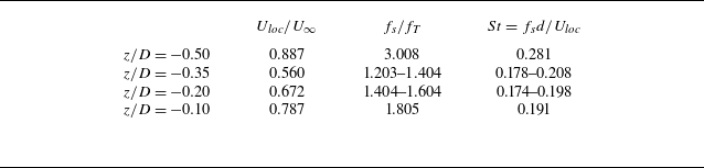
Table 2. Long description
A table with four rows and three columns comparing local Strouhal numbers for different tower-side pressure probes. The columns are labeled U_loc / U_infinity, f_s / f_T, and St. The row labels are z / D with values -0.50, -0.35, -0.20, and -0.10. Row 1: U_loc / U_infinity, 0.887; f_s / f_T, 3.008; St, 0.281. Row 2: U_loc / U_infinity, 0.560; f_s / f_T, 1.203-1.404; St, 0.178-0.208. Row 3: U_loc / U_infinity, 0.672; f_s / f_T, 1.404-1.604; St, 0.174-0.198. Row 4: U_loc / U_infinity, 0.787; f_s / f_T, 1.805; St, 0.191.
These results clearly highlight the distinct nature of the pressure fields acting on the rotor and the tower, respectively, and indicate that the BTI phenomenon may play a significant role in the acoustic characterization of a complete wind turbine. This aspect is further investigated in the following § 4.
3.1. Wind turbine wake
We now examine the characteristics of the wake up to
 $5D$
. We report the instantaneous vorticity component in the
 $y$
-direction and the phase-averaged TKE, computed from the three velocity fluctuation components, on the meridian
 $x{-}z$
plane passing through the origin of the frame of reference (figure 9
a and 9
b); figure 9(b) also contains the three-dimensional wake structure identified through the isosurface of the non-dimensional second invariant
 $Q$
of the velocity gradient tensor. It is defined as
 \begin{align} \frac {{\textit{QD}}^2}{U_\infty ^2} = \frac {D^2}{2U_\infty ^2}\left(\|M\|^2-\| N\|^2\right)\!, \end{align}
where
 $N$
and
 $M$
are the symmetric and deviatoric parts of the velocity gradient tensor, respectively. The phase-averaging of a generic variable
 $\varPsi$
is defined as
 \begin{align} \hat {\varPsi }(\boldsymbol {x}) = \frac {1}{N} \sum _{k=1}^{N} \varPsi (\boldsymbol {x}, t_0 + k\varDelta t), \end{align}
where
 $\varDelta t = 1/(3f_T)$
is the time interval of the phase,
 $N=15$
. Here,
 $N=15$
denotes the number of phase-conditioned snapshots available over the five rotor revolutions. This average is used only as a qualitative visualization of the phase-organized wake structures, and not as a statistically converged estimate of turbulent second-order quantities.
(a) Instantaneous vorticity component in the
 $y$
-direction normalized with
 $U_\infty /R$
in the meridian plane passing through the wind turbine axis. (b) Snapshots of isosurfaces
 ${\textit{QD}}^2/U_\infty ^2=126$
in the three-dimensional space and phase-averaged TKE on the meridian plane, normalized using
 $U_{\infty } ^2$
.

The visualization of the instantaneous Q and vorticity fields (figure 9) shows a wide variety of small vortical structures populating the wake and coexisting with the helicoidal system of tip vortices, the blade wake, the root vortices and the tower’s wake. Consequently, a highly complex flow field arises, involving a wide range of interacting temporal and spatial scales, as previously highlighted by Biswas & Buxton (Reference Biswas and Buxton2024a). In particular, the instantaneous vorticity field, shown in figure 9, exhibits a noticeable similarity to that obtained in the experiment of Biswas & Buxton (Reference Biswas and Buxton2024a) (compare with their figure 2a). Several vortical structures are present in the wake, unlike the IR case, where the coherent structures seem to be more organized in the near wake (compare figure 9 b with figure 12 of RPCA25).
The complexity of the flow field is clearly visible in the Supplementary movie 1 is available at https://doi.org/10.1017/jfm.2026.12018, in which the magnitude of the dimensionless vorticity field is reported over the meridian plane; it is the result of the superposition of multiple fluid-dynamic structures characterized by different temporal and spatial scales, intrinsic asymmetry and strong three-dimensionality, making the definition of near, intermediate and far wake regions less straightforward than in the case of an IR. In RPCA25, the near, intermediate and far wake regions were defined consistently with the evolution of the tip-vortex system. In particular, the near wake corresponds to the region where strong coherent structures are still clearly identifiable. The intermediate wake is characterized by the progressive destabilization of the tip-vortex system, leading to the generation of smaller turbulent structures. Finally, in the far wake, these structures spread and eventually occupy the entire cross-section of the wake. This classification is consistent with the physical evolution of the wake and provides a clear link between the underlying fluid-dynamic processes and noise generation and propagation in the case of an IR. This is justified by the fact that wake development is predominantly governed by the tip-vortex system and its instability mechanisms.
On the other hand, when the tower is present, BTI affects the evolution of the wake, promoting a more rapid transition from near to far wake through different fluid dynamic processes evolving in different parts of the wake.
Biswas & Buxton (Reference Biswas and Buxton2024a) proposed a robust definition of two regions of the wake, based on the relative strength between the tip vortex system and the wake meandering process. The authors defined a convective step length scale
 $L_c = \pi D/TSR$
, and showed that at a distance of around
 $3L_c$
the strength of the wake meandering overcomes that of the tip vortex system, defining the end of the near wake.
Having established this reference framework, we now turn our attention to the flow organization. In particular, we examine the coherent flow structures that characterize the turbulent wake before their progressive destabilization and the consequent loss of phase-locking with the rotor motion, with the aim of clearly identifying the transition between the near and the far wake. In the configuration of a complete wind turbine, the presence of the tower breaks the axial symmetry of the problem, making the analysis based on a single phase inherently less representative of the overall flow dynamics. In particular, for a three-blade rotor, two significant phases can be identified: the first corresponds to the blade positioned vertically upward, while the second occurs when the blade passes directly in front of the tower. We calculated the statistics for the two phases and observed that the results relative to the latter phase (not shown here) do not exhibit substantial differences with respect to those relative to the first one; for this reason, here we discuss the first one.
Phase-averaged fields of mean streamwise velocity, vorticity magnitude and TKE are reported over: the meridian plane (figure 10); a series of cross-sectional planes located at increasing downstream distances from the wind turbine (figure 11); horizontal planes positioned at
 $z/D = \pm 0.25$
(figure 12).
The analysis of the phase-averaged quantities reveals that the complexity of the wake is governed by the dynamics and instability of the tip vortex system as well as by the presence of the tower and of its wake.
Phase-averaged quantities in the meridian plane passing through the wind turbine axis: (a) axial velocity field normalized with
 $U_\infty$
; (b) vorticity in the
 $y$
-direction normalized with
 $U_\infty /R$
; (c) TKE normalized with
 $U_\infty ^2$
.

Phase-averaged axial velocity (a,d,g,j,m), vorticity magnitude (b,e,h,k,n) and TKE (c,f,i,l,o) normalized using
 $U_{\infty }$
and
 $R$
. From (a)–(c) to (m)–(o), each row of panels corresponds at a certain distance downstream the wind turbine:
 $x/D = 0.2$
;
 $0.4$
;
 $1.0$
;
 $2.0$
;
 $4.0$
.

Phase-averaged quantities in horizontal planes positioned at (a,c,e)
 $z/D = - 0.25$
and (b,d,f)
 $z/D = 0.25$
: (a,b) axial velocity field normalized with
 $U_\infty$
; (c,d) vorticity in the
 $y$
-direction normalized with
 $U_\infty /R$
; (e,f) TKE normalized with
 $U_\infty ^2$
.

The extraction of kinetic energy by the wind turbine produces a momentum deficit, visible in figure 10(a) through the corresponding streamwise velocity deficit. The latter is mainly concentrated between the hub and the blade-tip trajectory, leading to the characteristic double-bell shape of the wake velocity profile and to the progressive expansion of the wake downstream.
The geometry of the wind turbine promotes the generation of a high-speed jet with an initial velocity higher than
 $U_\infty$
that extends up to
 $2D$
behind the hub. It is important to note that the jet is more pronounced and persists for a longer distance up to approximately
 $5D$
in the case of an IR (see figure 9 of RPCA25). A similar behaviour was observed by Santoni et al. (Reference Santoni, Carrasquillo, Arenas-Navarro and Leonardi2017), Debnath et al. (Reference Debnath, Santoni, Leonardi and Iungo2017) and De Cillis et al. (Reference De Cillis, Cherubini, Semeraro, Leonardi and De Palma2021), who emphasized that neglecting the tower and nacelle results in a non-physical jet in the central region. On the other hand, in view of our results, for both the IR and the complete machine, this jet cannot be classified as non-physical, rather its presence and intensity depend on the geometrical properties of the wind turbine, confirming the importance of the near-hub rotor design, as already pointed out by other authors (see, among them, Kang et al. (Reference Kang, Yang and Sotiropoulos2014)).
In the lower part of the wake (figure 10), a strong momentum deficit is present behind the tower, which is related to the tower-induced wake and its nonlinear interaction with the blade wake, making the flow substantially different and more complex with respect to the IR case. This is even more evident looking at the cross-sectional plane placed at
 $x/D = 0.2$
(figure 11
a), in which it is clear that the momentum deficit is more pronounced in the region behind the tower, while the axial velocity exhibits a maximum at the blade tip.
The near wake is dominated by organized coherent structures, including the tip-vortex system, the thin trailing-edge vortex sheet and the root vortices (figure 10
b), resembling those observed for the IR. These features are clearly visible in the upper meridian plane up to
 $ \sim\!1.2D = 1.8 L_c$
, slightly smaller than the value of
 $3L_c$
suggested by Biswas & Buxton (Reference Biswas and Buxton2024a). This difference might be attributed to the different geometry of the wind turbine blade and to the different Reynolds numbers considered here.
The cross-sectional view at
 $x/D = 0.2$
(figure 11
b) further confirms that, in this very near-wake region, the wake of the blades, the root vortices and the tower-induced wake remain distinct and coherent throughout the section. As the distance downstream increases (
 $x/D = 0.4$
), the streamwise velocity remains high near the blade tips, while the velocity deficit becomes more uniformly distributed within the annular region between the hub and the tip. In contrast, the velocity deficit in the tower wake is less pronounced than in the rotor wake for the present idealized uniform inflow configuration (figures 11
d). This result should be interpreted with caution, since the absence of an atmospheric boundary layer and of a no-slip ground boundary layer likely accelerates the recovery of the lower wake. Under realistic atmospheric inflow conditions, the reduced momentum supply near the ground is expected to delay the tower wake recovery. The system of tip vortices still exhibits some coherence, as evidenced by the large values of vorticity and TKE at the outer radii, while in the lower region, the tower’s vortex shedding, the blade wake and the root vortices interact with each other, promoting asymmetry in the fluid flow (look at figure 11
d,f and figure 12
a,c,e). An intense vortical structure sheet, characterized by strong vorticity and TKE, is generated by this nonlinear interaction, which is transported to the right and upwards, due to the clockwise rotation of the wind turbine. This phenomenon is already emphasized by, among others, Santoni et al. (Reference Santoni, Carrasquillo, Arenas-Navarro and Leonardi2017), Debnath et al. (Reference Debnath, Santoni, Leonardi and Iungo2017) and De Cillis et al. (Reference De Cillis, Cherubini, Semeraro, Leonardi and De Palma2021). This interaction becomes more and more evident as the distance increases, promoting a decrease in the vorticity magnitude and increased mixing, which corresponds to the slight rise of TKE, more intense in the root, and in the tip region behind the tower (figure 11
g–i). Finally, the interaction leads to the transport of TKE mainly in the right-hand part of the wake cross-section; specifically, TKE starts to be spread over the entire right-hand half-plane at
 $x/D \approx 2.0$
(figure 11
j–l), although still more concentrated and intense at the outer radii. The scenario is evidenced in figure 12, which shows that, approximately at
 $x/D \approx 2.0$
in the lower part of the wake (figure 12
a,c,e), the wake generated by the tower begins to interact with the rotating system of tip vortices at the right-hand part of the outer radii of the wake and starts to be transported along the wake rotation. In other words, the wake of the tower, while moving downstream, is transported by the rotational motion, giving rise to a sort of helicoidal wake (see figure 12
c–f).
At the same time, in the region within
 $1-2D$
downstream of the rotor, a decrease of vorticity at the outer radii of the wake corresponds to an increase in TKE (more evident in the upper plane, figure 10), initially at
 $x/D \sim 1.0$
, where the tip vortices start to lose coherence. The TKE is then transported and spread across the annular outer region at
 $x/D = 2.0$
(figure 11
i,l), indicating a mutual interaction among the tip vortices (figure 9), leading to the mechanisms of vortex grouping ((Felli et al. Reference Felli, Camussi and Di Felice2011; Posa et al. Reference Posa, Broglia and Balaras2021) RPCA25).
Moving downstream, the far-wake region is characterized by an increasingly uniform distribution of axial velocity and TKE across the rotor disk (figure 11 m–o), resulting from the complex interaction between the wake of the tower and the rotational wake of the rotor discussed above. Moving farther downstream, it is also evident that the wake tends to exhibit axial symmetry, indicating the tendency to lose memory of the wake generator, promoting a more homogeneous turbulent flow.
Overall, the phase-averaged analysis highlights the presence of two distinct physical mechanisms governing the dynamics of the transition from the near to the far wake of the complete wind turbine configuration. The first one is associated with the evolution and instability of the tip-vortex system. This mechanism closely resembles the behaviour observed for the IR, where tip vortices progressively lose coherence through mutual interaction, vortex grouping and merging, ultimately leading to the breakdown of phase-locked large-scale structures. As documented in previous studies and confirmed here, this process becomes particularly evident in the region
 $x/D \approx 1$
–
 $2$
(Biswas & Buxton Reference Biswas and Buxton2024a
, Reference Biswas and Buxtonb).
The second mechanism is related to the presence of the tower and dominates the lower part of the near wake. In this region, the vortex shedding generated by the tower interacts nonlinearly with the blade wakes, root vortices and the rotating tip vortex system. This interaction promotes strong asymmetry, enhanced mixing and the formation of coherent vortical structures that are convected and distorted by the wake’s rotational motion.
4. Results and discussion: acoustic analysis
4.1. The noise sources
As in RPCA25, here we analyse the pressure fluctuation field over the solid surfaces responsible for the loading part of the noise. In this case, the analysis considers the presence of the rotor and of the tower. We discuss the root-mean-square (r.m.s.) of the non-dimensional pressure fluctuations on a single blade and on the tower calculated over five periods of rotation (figures 13 and 14).
As for the IR case, the downwind side of the blade is found to experience fluctuations more energetic than the upwind one, associated with laminar–turbulent transition and flow separation. Significant pressure fluctuations are also detected near the trailing edge and increase moving towards the tip region, where the local chord-based Reynolds number is higher. At the blade tip (figure 13 c), the interaction with the tip vortex generates additional fluctuations, albeit weaker than those at the trailing edge. This is in line with observations of RPCA25, and suggests that the trailing edge remains the dominant high-frequency noise source, as also pointed out by Wagner et al. (Reference Wagner, Bareiss and Guidati1996).
The r.m.s. of the pressure fluctuation field normalized with
 $ \rho _0 U_\infty ^2$
on the blade’s surface: downwind side (a); upwind side (b); tip of the blade (c).

The r.m.s. of the pressure fluctuation field normalized with
 $\rho U_\infty ^2$
on the tower’s surface: downwind side (a); upwind side (b).

Time history of the POD coefficients calculated using the pressure field on the blade: (a) first mode; (b) second mode. Spectra of the POD coefficients: (c) first mode; (d) second mode. Spatial modes: (e) first POD mode; (f) second POD mode.

Pressure fluctuations are also visible on the surface of the tower, although with intensity lower than that observed over the blade (figure 14). These fluctuations are mainly associated with the interaction between the blade and the tower and, consequently, are more energetic in the central and near-hub regions. The pressure fluctuations on the upwind face of the tower are slightly higher than on the downwind face due to the blade passage. The inviscid process associated with the passage of the blade over the tower, together with the nonlinear interaction between the tip vortex, the trailing edge vortex sheet and the root vortices with the tower boundary layer promote higher pressure fluctuations compared with the isolated tower; this can be inferred looking at the lower part of the tower, where the pressure fluctuations are negligible compared with the central and upper part.
To further elucidate the role of BTI in the generation of pressure fluctuations, a POD analysis (Chatterjee Reference Chatterjee2000) is applied to the pressure field on both the blade and the tower (figures 15 and 16, respectively). Figure 15 reports the first two dominant POD modes for the blade surface. The temporal coefficients and their corresponding spectra (figure 15 a–d) reveal a pronounced broadband content at high frequencies, which is consistent with the development of a separated turbulent boundary layer, likely promoted by the relatively low chord Reynolds number of the present configuration. This interpretation is supported by the spatial structure of the modes (figure 15 e–f), characterized by small-scale fluctuations distributed along the blade surface, especially near the trailing edge and more intense moving towards the tip of the blade. The flow over the blade was further examined through the projected wall-shear coefficient
 \begin{align} C_{f,c} = \frac {\boldsymbol{\tau }_w \boldsymbol{\cdot }\boldsymbol{e}_c} {\frac {1}{2}\rho U_\infty ^2}, \end{align}
where
 $\boldsymbol{\tau }_w$
is the wall-shear-stress vector and
 $\boldsymbol{e}_c$
is the local chordwise unit vector, oriented from the leading edge to the trailing edge. The analysis shows localized regions on the downwind side of the blade, close to the trailing edge, where
 $C_{f,c}\lt 0$
. This indicates a local reversal of the wall-shear direction and suggests the presence of separated flow. This is also confirmed by line-integral-convolution visualizations of the velocity field in the blade sections, which clearly show separated-flow regions close to the airfoil surface near the trailing edge. These diagnostics support the physical interpretation of the pressure modes, but are not reported in detail in order to keep the discussion focused on the acoustic-source mechanisms. In addition, the first temporal mode exhibits a marked modulation at the revolution frequency, indicating that the passage in front of the tower induces a periodic modification of the blade aerodynamics due to the reduced-velocity region generated upstream of the tower. This behaviour is consistent with the time evolution of the thrust discussed in the previous section.
Figure 16 highlights the tonal character of the pressure field acting on the tower as a consequence of BTI. The first POD mode (figure 16
a,c,e) clearly captures the sharp pressure variation occurring at the BPF and at its superharmonics. The largest pressure fluctuations are localized on the upwind face of the tower, directly evidencing the BTI mechanism. The wake shed by the blade is advected downstream and impinges on the tower’s upwind surface, producing enhanced unsteady loading and significantly altering the local boundary-layer dynamics. The second mode exhibits periodic behaviour predominantly governed by the vortex shedding process. Its spatial organization (figure 16
g,h) displays the canonical alternating shedding pattern, while the spectra of the associated temporal coefficient show a concentration of energy around the theoretical vortex shedding frequency (
 $f_{VS} \approx 1.5 f_T$
). The presence of energy distributed over a finite frequency band highlights the non-monochromatic nature and the height-dependent nature of the shedding process as already argued in § 3. Finally, it is worth noting that both POD modes exhibit asymmetry in their spatial distribution, suggesting a non-symmetric preferential direction of noise propagation, as discussed in the next section.
Time history of the POD coefficients calculated using the pressure field on the tower: (a) first mode; (b) second mode. Spectra of the POD coefficients: (c) first mode; (d) second mode. Spatial modes: (e,f) first POD mode; (g,h) second POD mode.

Phase-averaged r.m.s. of the Lighthill source term made non-dimensional with
 $\varOmega ^2$
: (a) complete configuration; (b) the IR case.

In figure 17 we report the r.m.s. of the phase-averaged kinematic Lighthill source term over the meridian plane, for the IR case and the complete configuration, to quantify the major noise source associated with the wake, mainly at the BPF. The kinematic Lighthill source term is
 \begin{align} S = \frac {\partial ^2 u_i u_{\!j}} {\partial x_i \partial x_{\!j}}. \end{align}
The analysis of the figure 17 shows that, in the near wake, significant noise sources at the blade-passing frequency are associated with the tip and root vortices, with the trailing edge vortex sheet and with the tower’s wake, the latter is not present in the IR case; the intensity of these sources rapidly decreases moving downward along the wake, consistently with a strong decay of vorticity in this region. Beyond
 $x \sim 1.2 D$
, the noise sources are predominantly concentrated within the tip vortex region and progressively extend to cover the entire rotor disc in the farthest region of the wake. Differences between the IR case and the complete configuration are evident in terms of spatial distribution of the source rather than in the intensity of the Lighthill source term; however, it is worth mentioning that the power spectral density of the acoustic pressure is directly related to the two-point cross-spectral densities of the Lighthill stress tensor (for more details see, among others, Kerhervé et al. (Reference Kerhervé, Fitzpatrick and Jordan2006), Bogey & Bailly (Reference Bogey and Bailly2007), Cavalieri & Agarwal (Reference Cavalieri and Agarwal2014) and Karban et al. (Reference Karban, Bugeat, Towne, Lesshafft, Agarwal and Jordan2023)) and then a direct comparison of the Lighthill source term fluctuations alone does not provide a complete assessment of the relative strength of the nonlinear acoustic sources in the two configurations.
To summarize, at the BPF, in the very near field downstream of the turbine, the complex fluid dynamic field resulting from the BTI constitutes a noise source comparable to the one associated with the tip vortex structure; conversely, moving downstream, the fluid dynamic disturbances associated with the tip vortex dynamics remain the most relevant noise source in the wake.
4.2. Acoustic spectra
In this section, we highlight the role of the tower and BTI correlating the main fluid-dynamic processes with noise generation; we focus on the differences between the IR case (RPCA25) and the present case, under the assumption of an infinite homogeneous medium (i.e. in the absence of the bottom reflection plane).
We calculate the linear and the nonlinear contributions to the sound pressure level (SPL) of the acoustic pressure
 $\hat {p}$
at the arrays of microphones depicted in figure 5 and placed as follows: three stand along the streamwise direction,
 $x/D = 0.0, 1.0, 2.0$
at
 $y/D=0$
,
 $z/D = 1.0$
(ARRAY I); three stand along the lateral direction,
 $y/D = 2.0, 4.0, 8.0$
at
 $x/D=0, z/D=0$
(ARRAY II); three stand along the vertical direction upward,
 $z/D = 2.0, 4.0, 8.0$
(ARRAY III), in the rotor plane (
 $x/D = 0.0$
,
 $y/D=0$
). For clarity and direct comparison, the overall acoustic spectra of the IR case are also reported. The SPL is defined as in RPCA25 reads
 \begin{align} \textit{SPL} = 20 \log _{10} \left (\frac {\textit{fft}(\hat p)}{ \hat p_0}\right )\!, \end{align}
where
 $\textit{fft}$
is the fast Fourier transform of
 $\hat p$
and
 $\hat p_0 = 20 \mu \textrm {Pa}$
is the SPL in air. A comparison between the zero-delay and retarded-time evaluations, the latter performed using the advanced-time approach (see Casalino (Reference Casalino2003) for more details), showed that the inclusion of propagation delays does not significantly modify the spectra or directivity patterns discussed here for the linear contribution. Therefore, in the following results we neglect time-delay effects. This approximation is consistent with the estimates reported in RPCA25, according to which time-delay effects are expected to affect only frequencies above approximately
 $30f_T$
for the linear terms. Moreover, the retarded-time treatment of the nonlinear contribution is considerably more complex and computationally demanding. The acoustic spectra for the three arrays are shown in figure 18. Peaks at the BPF and at its superharmonics are clearly observed in both the linear and nonlinear contributions; their amplitudes tend to decrease with increasing distance from the source. The linear component dominates the SPL across most of the frequency range, except at lower frequencies as the distance from the source increases. This phenomenon is particularly evident in the streamwise direction, as in the IR case. For the microphones of ARRAY I, close to the turbine, no significant differences are detected between the IR case and the complete turbine; on the other hand, with increasing distance along the streamwise direction, a significant difference emerges between the two configurations within the frequency band (
 $0{-}4f_T$
) (figure 18
c).
Linear (red lines) and nonlinear (blue lines) noise contributions, together with the total noise, expressed in terms of SPL of the acoustic pressure. (a–c) Microphones of ARRAY I (
 $x/D=0.0 ; \; 1.0 ; \; 2.0$
); (d–f) microphones of ARRAY II (
 $y/D=2.0 ; \; 4.0 ; \; 8.0$
); (g–i) microphones of ARRAY III (
 $z/D=2.0 ; \; 4.0 ; \; 8.0$
). The dashed black line denotes the overall SPL of the IR case (I–R) at the same microphones. The shaded grey region highlights the frequency range in which compressibility-delay effects may influence the evaluation of the nonlinear terms. Here, ‘overall’ denotes the total (linear and nonlinear) acoustic contribution of the complete-turbine configuration, whereas ‘IR’ denotes the corresponding overall acoustic contribution of the isolated-rotor case.

In particular, for the complete turbine configuration, the low-frequency range dominated by the nonlinear contribution is both narrower and weaker, remaining confined around the rotor revolution frequency. In contrast, in the IR case, it extends up to approximately
 $3f_T$
and is significantly more pronounced. As already emphasized in the previous section, the destabilization of the complete wind turbine wake is promoted by two main physical mechanisms: one is associated with the tip vortex instability, and the other is associated with the presence of the tower-induced wake, which interacts with the blade wake, the tip and root vortices. In the IR case, wake destabilization is confined in the tip region of the intermediate wake, mainly associated with tip vortex instability and the vortex grouping process. For both configurations, the wake destabilization enhances mixing and development of broadband turbulence; as a consequence, a transition occurs from a predominantly tonal acoustic spectrum to a more broadband one. The main difference between the two configurations is the degree of coherence and the organization of the near wake, which is more evident and persists longer in the IR case compared with the complete configuration.
As already mentioned, the power spectral density of the acoustic pressure is defined as the Fourier transform of its autocorrelation function and can be expressed in terms of the two-point cross-spectral density of the source as follows (e.g. Cavalieri & Agarwal (Reference Cavalieri and Agarwal2014)):
 \begin{align} \left \langle \hat {p}(\boldsymbol{x},f) \hat {p}^*(\boldsymbol{x},f) \right \rangle = \iint _V G_{\textit{ij}}(\boldsymbol{x},\boldsymbol{y},f)\, G^*_{kl}(\boldsymbol{x},\boldsymbol{y}',f)\, R_{ijkl}(\boldsymbol{y},\boldsymbol{y}',f) \, \text{d}\boldsymbol{y}\, \text{d}\boldsymbol{y}' ,\end{align}
where
 $\langle \boldsymbol{\cdot }\rangle$
denotes an ensembling (or time) averaging operation,
 \begin{align} R_{ijkl}(\boldsymbol{y},\boldsymbol{y}',f) = \left \langle \hat {T}_{\textit{ij}}(\boldsymbol{y},f)\, \hat {T}^*_{kl}(\boldsymbol{y}',f) \right \rangle \end{align}
is the two-point cross-spectral density of the Lighthill stress tensor,
 $G_{\textit{ij}}(\boldsymbol{x},\boldsymbol{y},f)$
is the Green function and
 $^*$
denotes a complex conjugate quantity. This formulation highlights that the acoustic field is governed by the spatial and temporal correlation of the source term. Consequently, the higher level of coherence and organization of the wake in the IR case promotes stronger low-frequency acoustic radiation, whereas the loss of coherence induced by the tower leads to a reduction of the nonlinear contribution.
To further characterize the spatial organization of the nonlinear source region, we consider the quadratic velocity tensor
 \begin{align} T_{\textit{ij}}(\boldsymbol{x},t)= u_i(\boldsymbol{x},t) u_{\!j}(\boldsymbol{x},t), \end{align}
which represents the dominant contribution to the Lighthill source term, and its Frobenius norm
 \begin{align} |T| = \left (T_{\textit{ij}}T_{\textit{ij}}\right )^{1/2} = |\boldsymbol{u}|^2. \end{align}
Here
 $u_i$
denotes the resolved (LES-filtered) velocity, and the subgrid contribution to the source is not included in this diagnostic. For a selected seed point
 $\boldsymbol{x}_{\!s}$
in the wake, the temporal fluctuation of this quantity is defined as
 \begin{align} |T(\boldsymbol{x},t)|' = |T(\boldsymbol{x},t)| - \left \langle |T(\boldsymbol{x})| \right \rangle \!, \end{align}
where
 $\langle \boldsymbol{\cdot }\rangle$
denotes averaging over the sampled time window. We then compute the normalized two-point correlation field
 \begin{align} R_{|T|}(\boldsymbol{x}_{\!s},\boldsymbol{x}) = \frac { \left \langle |T(\boldsymbol{x}_{\!s},t)|' |T(\boldsymbol{x},t)|' \right \rangle }{ \left [ \left \langle |T(\boldsymbol{x}_{\!s},t)|'^2\right \rangle \left \langle |T(\boldsymbol{x},t)|'^2\right \rangle \right ]^{1/2} }. \end{align}
Comparison of
 $R_{|T|}$
correlation maps for the isolated-rotor (a) and complete-turbine (b) configurations at probe location
 $x/D=1, z/D=0.5$
, over the meridian plane.

By construction,
 $R_{|T|}(\boldsymbol{x}_{\!s},\boldsymbol{x}_{\!s})=1$
. This quantity is not intended to reconstruct the full acoustic convolution of the Lighthill source term, which would require the two-point cross-spectral tensor between all source locations. Rather, it provides a local diagnostic of the spatial coherence. In figure 19, we report the two-point correlation field for a seed point located at
 $x/D = 1$
and
 $z/D = 0.5$
, over the meridian plane, for the IR case and the complete configuration, respectively. For the IR case, the two-point correlation of the source exhibits an organized, quasiperiodic wake structure in the near wake, up to
 $x/D \approx 1$
for the seed point considered here. Moreover, this structure is approximately symmetric about the wake axis (
 $z/D = 0$
). In contrast, for the complete configuration the organized wake structure, that characterizes the isolated case near wake is largely absent, and the symmetry between the upper and lower parts of the wake is lost, indicating that the presence of the tower promotes strong decorrelation between them. Although this analysis is limited to the two-point correlation of the norm of the source proxy with respect to a prescribed seed point, it provides useful information on the spatial organization of the wake source region. It should not be interpreted as a formal quantification of the radiated noise at a given frequency, since that would require the full two-point cross-spectral source tensor over the entire source volume, together with the acoustic propagation kernels. Nevertheless, the present diagnostic indicates that the presence of the tower distorts the coherent organization of the rotor wake and promotes a more asymmetric and decorrelated source region. This supports the interpretation that the tower modifies the spatial distribution of the nonlinear acoustic sources, although a complete two-point source-coherence analysis is beyond the scope of the present work and should be addressed in a dedicated future study. This behaviour highlights the role of the tower in reducing wake coherence and large-scale flow organization.
Along the lateral direction (
 $y$
), in the rotor plane (ARRAY II) (figure 18
d–f), significant differences between the two configurations are evident in the medium frequency range (
 $1{-}10f_T$
). To be noted that along the lateral direction, the linear part of the noise dominates; in particular, for the complete turbine, the BPF and superharmonic peaks remain clearly visible up to
 $8D$
, associated with the tonal character of the pressure fluctuations over the tower, induced by BTI. Conversely, the noise contribution at the BPF in the IR case tends to vanish moving towards the far field. In addition, there is a pronounced amount of acoustic energy around
 $1.5 f_T$
, which can be attributed to the tower’s vortex shedding (see figures 8 and 14), obviously absent in the case of the IR. This clearly demonstrates that the tower plays a significant role in the lateral direction, a point that will be further analysed later in this section. It should be noted that the fundamental peak at the blade passage frequency for the overall noise is slightly smaller than that of the linear noise and higher than that of the nonlinear terms. This phenomenon was already observed in RPCA25 for the IR case. This happens because the overall noise is not an algebraic sum of linear and nonlinear contributions (in terms of r.m.s. of the time signals); rather, the time signals of the linear and nonlinear noise are not synchronized with the same phase, sometimes causing a destructive autointeraction between the linear and nonlinear noise sources.
Finally, in the vertical direction upward (ARRAY III, figure 18 g–i), the spectra are mainly dominated by the linear contribution, out of the very low frequency range, as in the IR case. Significant differences between the two cases are not present, pointing out that in the vertical direction upward, the tower plays a marginal role.
Rotor (red lines) and tower (blue lines) contributions to the linear noise in terms of SPL of acoustic pressure. (a–c) Microphones of ARRAY I (
 $x/D=0.0 ; \; 1.0 ; \; 2.0$
); (d–f) microphones of ARRAY II (
 $y/D=2.0 ; \; 4.0 ; \; 8.0$
); (g–i) microphones of ARRAY III (
 $z/D=2.0 ; \; 4.0 ; \; 8.0$
). The dashed black line denotes the overall SPL of the IR case at the same microphones. Here, ‘overall’ denotes the total linear acoustic contribution of the complete-turbine configuration, obtained from all solid surfaces included in the FWH calculation, whereas ‘IR’ denotes the corresponding linear acoustic contribution of the isolated-rotor case.

Figure 20. Long description
Nine line graphs depict sound pressure levels (SPL) from different sources in wind turbine noise experiments. Each graph shows SPL in decibels (dB) on the vertical axis and the frequency ratio (f/f_T) on the horizontal axis. Panel A, Panel B, and Panel C correspond to microphones of ARRAY I. Panel D, Panel E, and Panel F correspond to microphones of ARRAY II. Panel G, Panel H, and Panel I correspond to microphones of ARRAY III. Each graph includes red lines representing rotor contributions and blue lines representing tower contributions to the linear noise. The dashed black line denotes the overall SPL of the IR case at the same microphones. The graphs show variations in SPL across different frequency ratios, with notable peaks and troughs indicating specific noise characteristics. The overall trend shows that rotor contributions generally have higher SPL values compared to tower contributions.
A question now arises on the relative importance of the tower versus the rotor for the linear contribution to the noise, which, as discussed in the analysis of figure 18 plays a dominant role in a wide range of frequencies. The single contributions of the rotor and the tower are depicted in figure 20, which shows the spectra for the three arrays already discussed along the
 $x$
-,
 $y$
- and
 $z$
-directions, respectively. For the sake of clarity, in that calculation, the nacelle was considered in the rotor contribution, and it plays a marginal role.
Along the wake (ARRAY I), the rotor contributes the most to the overall linear acoustic footprint; both exhibit a tonal behaviour at the BPF and superharmonics, making evident the importance of BTI regarding the pressure distribution over the tower rather than the tower’s vortex shedding, as expected from the previous analysis on noise sources (see figure 14). The contribution of the tower becomes increasingly significant moving downstream along the wake (compare figures 20
a and 20
c).This behaviour may be mainly ascribed to a geometric projection effect. In particular, moving downstream, the radiation direction from the tower to the observer becomes increasingly aligned with the streamwise direction, so that the projection factor entering the loading term,
 $\hat n_i \hat r_i$
, becomes larger. Therefore, the tower contribution initially increases in the streamwise direction and then decays as acoustic propagation proceeds.
Along the
 $y$
-direction (ARRAY II), the overall linear acoustic footprint is dominated by the tower, apart at the BPF where the two elements contribute roughly the same. The tower contributes the most around
 $1.5f_T$
, as further confirmation that, in this direction, the pressure induced over the tower by vortex shedding constitutes a significant noise source.
Finally, along the vertical upward direction (ARRAY III), the contribution of the tower is irrelevant (figure 20 g–i), again associated with geometrical features.
These results make it evident that, regarding the linear part of the acoustic footprint, the rotor and the tower are expected to exhibit different directivity patterns.
4.3. Directivity and decay rate
In RPCA25, the authors highlighted that for the IR, the nonlinear noise component may play a role in the near field, and, as the distance increases (
 $K_\lambda = d/\lambda \gt 1$
, where
 $d$
is the distance from the source and
 $\lambda = c_0 /3f_T$
), the linear terms become dominant. In the case of the complete wind turbine, similar results are expected. Therefore, in this context, we aim to highlight the role played by the presence of the tower and the reflection plane on the directivity of the noise pattern and the acoustic decay rate, considering five revolution periods.
Figure 21 reports the directivity patterns (in decibels) over a circle of radius equal to
 $10D$
placed in the horizontal
 $x{-}y$
plane passing through the centre of the rotor, for the complete turbine and for the IR of RPCA25. For both linear and nonlinear contributions, significant differences in amplitude between the two configurations are observed, particularly in the lateral direction.
At the distance from the sources herein considered, which gives
 $K_\lambda = 1.1$
, the linear contribution dominates the overall noise, as in the IR case, and it displays an oval-shaped directivity pattern elongated in the streamwise direction (figure 21
a), different from the canonical dipole shape typical of the IR case. Also, the linear noise part exhibits a clear asymmetry with respect to the streamwise direction (
 $0^\circ$
–
 $180^\circ$
), consistent with previous findings reported in Yauwenas et al. (Reference Yauwenas, Zajamšek, Reizes, Timchenko and Doolan2017, Reference Yauwenas, Zajamšek, Reizes, Timchenko and Doolan2021) and with the experimental measurements performed by Duc & Finez (Reference Duc and Finez2025); as also discussed in the literature, such behaviour has to be attributed to BTI and, specifically, to asymmetry introduced by the interaction between rotation and the tower.
Directivity of r.m.s. of acoustic pressure fluctuations
 $\hat {p}'_{\text{\em rms}}$
(dB) at microphones placed in concentric circle (
 $10D$
) on the
 $x{-}y$
plane passing through the centre of the rotor. (a) Linear contribution; (b) nonlinear contribution; (c) total contribution. (d) Linear contribution from the rotor; (e) linear contribution from the tower; (f) total linear contribution. The arrow indicates the streamwise direction, and the dot–dash line is the result coming from the IR case.

The nonlinear component is approximately 20 dB lower than the linear one and shows a slightly different preferential radiation direction, with a more pronounced lobe aligned with the wake direction. This further confirms that the substantial differences in the wake between the two cases significantly affect the nonlinear acoustic signature. Overall (figure 21
c), the complete configuration generates higher noise levels in the
 $x$
–
 $y$
plane compared with the IR case, while the directivity pattern tends to deviate from the classical dipole shape towards an oval and slightly asymmetric distribution. Although the increase in overall noise levels can be mainly attributed to the presence of the tower, the modification of the directivity pattern is mainly associated with the BTI, as shown in figure 21(d–f). The presence of the tower breaks the axial symmetry of the rotor aerodynamics, particularly when a blade passes through the velocity deficit region induced upstream of the tower. This interaction alters the local aerodynamic loading and the associated pressure field on the blade, producing an asymmetric acoustic radiation pattern. As a consequence, the rotor contribution itself (figure 21
d) exhibits a clear asymmetry along the streamwise direction. At the same time, the tower contribution is also inherently asymmetric in the horizontal plane. This behaviour can be associated with the non-uniform incoming flow over the tower due to rotation. As visible in the velocity field (figure 12
a,c,e), the tower wake does not develop strictly in the streamwise direction but appears slightly deflected. This feature is consistent with the observed asymmetry in the acoustic directivity and indicates the presence of an asymmetric pressure distribution acting on the tower, as already emphasized in the previous section (figure 16). Overall, the resulting acoustic radiation in the horizontal plane exhibits an almost isotropic character with a slight asymmetry resulting from the superposition of the dipole-shaped radiation generated by the rotor and a more isotropic distribution associated with the tower. It is also worth noting that, in the present configuration, the acoustic contributions of the rotor and the tower are of the same order of magnitude. Their relative importance may depend on the gap between the rotor and the tower, an aspect that deserves additional studies.
In the rotor plane (
 $y{-}z$
), linear and nonlinear contributions exhibit a dipole-shape and a nearly isotropic shape, respectively, with the former dominating in intensity over the latter. The total noise in this plane at
 $K_\lambda = 1.1$
is practically associated with its linear component (figure 22
a–c)
Directivity of r.m.s. of acoustic pressure fluctuations
 $\hat {p}'_{\text{\em rms}}$
(dB) at microphones placed in concentric circle (
 $10D$
) on the
 $y{-}z$
plane passing through the centre of the rotor. (a) Linear contribution; (b) nonlinear contribution; (c) total contribution. (d) Linear contribution from the rotor; (e) linear contribution from the tower; (f) total linear contribution.

Figure 22(d–f) show the contributions of the rotor and the tower to the linear part of the noise. As expected, the rotor contributes isotropically. Conversely, the tower exhibits a dipole shape that can be explained by the pressure distribution over its surface, discussed in the previous sections; further, the tower produces more noise in the lateral direction compared with the rotor, and consequently, the total linear noise directivity has a shape more similar to a dipole rather than a monopole, in the rotor plane. Our results exhibit some similarities with the propeller–rudder configuration studied in Posa et al. (Reference Posa, Broglia and Balaras2020) and Posa et al. (Reference Posa, Broglia, Balaras and Felli2023); there, the authors found that the rudder exhibits a dipole shape in the rotor plane with lobes elongated along the direction perpendicular to the symmetry plane of the rudder.
In figure 22, it can be noted that the monopole-shape and dipole-shape are not perfectly symmetric with respect to the vertical direction (
 $z$
-direction); this has to be attributed to the clockwise rotation of the wind turbine and BTI, which produced asymmetry in the pressure field as previously discussed.
The nonlinear part also exhibits an asymmetry with respect to the vertical direction, making the noise more intense on the right side of the wind turbine; again, this comes from the effect of rotational motion and the presence of the tower which makes the wake, on average not symmetric with respect to the meridian plane (see figures 12 and 11) as for the IR case.
Decay of the r.m.s. of acoustic pressure fluctuations
 $\hat {p}'_{\text{\em rms}}$
(dB): (a) decay along the streamwise direction out of the wake; (b) decay rate along the
 $y$
-direction; (c) decay rate along the
 $z$
-direction.

In figure 23 we show the decay rate of the linear, nonlinear and overall noise contributions along the
 $x$
,
 $y$
and
 $z$
directions up to
 $100D$
(
 $K_\lambda \approx 10.7$
), as already done for the IR case. In the streamwise and vertical upward directions, the results are qualitatively very similar to those of the IR case. Along the
 $y$
-direction, the decay rate of the linear term and, thus, that of the overall noise is quite different from that along the
 $z$
-direction as a further confirmation that the tower plays a major role in this direction compared with the other one, as already discussed. In particular, the distance at which the decay rate changes from the
 $r^{-4}$
behaviour to the
 $r^{-1}$
one is closer to the rotor, around
 $1.8D$
, as a further confirmation that the phenomenon of kinematic autointeraction (see Ianniello (Reference Ianniello2016), and RPCA25), promoted by the axial symmetry of the rotating source, is now broken by the presence of the tower which promotes a faster transition to the linear decay rate.
The nonlinear decay rate appears very similar to the case of the IR in both
 $y\text{-}$
and
 $z\text{-}$
directions, suggesting that the modifications on the wake produced by BTI do not play a significant role in this aspect. A significant difference, already emphasized in the previous section, is that the nonlinear contribution of the IR case is higher in the near wake (
 $1$
–
 $7D$
) compared with the complete configuration. This behaviour can be attributed to the higher coherence and persistence of organized coherent structures in the IR wake, whereas in the complete configuration, the interaction with the tower-induced wake promotes an earlier destabilization of these structures, enhancing mixing and dissipation and consequently reducing the strength of the nonlinear acoustic contribution.
4.4. The effect of the ground on acoustic reflection
In this section, we focus on the role played by the reflection plane on noise propagation. As established in the literature and confirmed by the present results (see the decay rate in figure 23), the nonlinear contribution becomes negligible compared with the linear component beyond a certain distance. Accordingly, the analysis is restricted to the linear term. As already presented in § 2, we take advantage of the method of images, considering the half-space Green function to model a complete reflective surface. Obviously, in a realistic environment, the ground is not a smooth, plane and fully reflective surface. However, as a first study of this effect, this model is representative of a typical scenario. In addition, reflection poses a significant challenge from the computational perspective, namely, quantification of the effect of the time delays given by the combination of direct and reflected signals. In particular, near the source, the delay between the direct and the reflected signals may have an effect on the acoustic spectra as well as on the directivity. For this reason, the acoustic postprocessing was also performed by explicitly including the retarded-time correction for the linear FWH contribution, using the advanced-time approach. The direct, reflected and overall linear signals were computed and compared with the compact, zero-delay approximation. This comparison, not reported here for brevity, showed negligible differences in the spectra and directivity trends discussed below for the present configuration, supporting the approximation of neglecting the effect of the time delay in the present analysis. Therefore, the results reported in the manuscript are those obtained under the zero-delay assumption.
The effect of the reflection plane is shown in figure 24, in which we report the directivity (at
 $K_\lambda = 1.1$
) considering propagation in an infinite medium and the presence of the ground, respectively. In the
 $x{-}y$
plane, it is evident that the presence of reflection brings a more intense noise, almost twice that of the infinite medium case, which corresponds to an increase of noise of approximately
 $6$
dB in all directions. On the rotor plane, reflection significantly changes the preferential direction of noise propagation, promoting a more evident dipole shape; this suggests that in the presence of the ground, noise propagates more in the lateral direction (
 $y$
-direction) rather than in the vertical one. To conclude, these outcomes reveal the significant effect of reflection due to the presence of the ground, always present in a realistic scenario.
Directivity of r.m.s. of acoustic pressure fluctuations
 $\hat {p}'_{\text{\em rms}}$
(dB) at microphones placed in concentric circles (
 $10D$
) on the
 $x{-}y$
plane (a) and
 $y{-}z$
(b). The diamond–solid line is the infinite medium case; the dot–dash line is the reflection plane case. The arrow indicates the streamwise direction.

5. Conclusions
As a natural extension of RPCA25, this study presents a comprehensive acoustic characterization of a model-scale wind turbine, including the tower and its impact on both the flow and the resulting acoustic field, using wall-resolving LES and acoustic analogy. The configuration is more representative of realistic operating conditions than that of an IR analysed in a large number of literature studies. Further, we model the ground as a fully reflective surface to highlight deviations from the idealized situation of noise propagation in an infinite homogeneous medium.
We use the same model-scale wind turbine as in the experimental campaign of GG23, except that the tower height is shorter than in the experiments and a uniform inflow velocity is prescribed. The uniform-inflow condition was retained to isolate the effect of the tower and to maintain consistency with the previously studied isolated-rotor configuration.
The time-averaged thrust and power coefficients are in good agreement with the experimental data, with the complete configuration providing a slightly closer match than the IR. Unlike the IR, the complete turbine exhibits a clear periodic response at the BPF, visible in both rotor and tower pressure-force contributions and associated with BTI. The rotor contribution is characterized by broadband high-frequency content related to turbulent/separated boundary-layer dynamics, whereas the tower response is mainly tonal, with peaks at the BPF and its harmonics. A low-frequency band around
 $1.5f_T$
is also observed and is compatible with tower vortex shedding, as supported by the local Strouhal estimate (
 $St \approx 0.2$
).
The flow analysis shows that the tower enhances wake asymmetry, promotes multiscale interactions and accelerates the transition from the near to the far wake. Two mechanisms are mainly responsible for this transition: tip-vortex instability and grouping, already observed in the IR, and the nonlinear interaction between the tower wake and the rotor wake, which is strongest in the lower part of the near wake.
The wall-pressure analysis and POD results indicate that blade pressure fluctuations are associated with broadband trailing-edge activity, modulated by BTI, while the tower pressure field is dominated by tonal components related to the blade passage and by a lower-frequency contribution consistent with vortex shedding. Finally, the analysis of the Lighthill source term confirms that the tower modifies the organization of the nonlinear source region, adding a further contribution to the near-wake acoustic source mechanisms.
In view of the fluid dynamics results, we analysed the acoustic field to relate the effect of the main fluid dynamic processes on acoustics. In the streamwise direction (
 $x$
), the linear and the nonlinear parts of the noise spectra exhibit a behaviour not very different from that of the IR near the source (
 $x/D \lt 2.0$
). On the other hand, significant differences arise in the low-frequency range (
 $0{-}4 f_T$
) with increasing distance from the turbine (
 $x/D \approx 2$
), where nonlinear noise contributions dominate. Compared with the IR, the complete configuration shows lower low-frequency nonlinear acoustic levels. This is attributed to the tower-induced distortion of the wake, which reduces the spatial coherence of the wake, as supported by the two-point correlation of the Lighthill source term. In the lateral direction (
 $y$
), the spectra are mainly dominated by the linear noise component, and significant differences are evident due to the role played by the tower. Especially, the BPF and superharmonics, together with the spread of energy around the tower vortex shedding frequency.
Finally, in the vertical
 $z$
-direction, upward, the results are very similar to the case of the IR, evidencing that the tower plays a marginal role. The analysis of the contribution related to the tower and the rotor, respectively, further confirms that the tower plays a significant role in the lateral direction and that rotor and tower produce different directivity patterns.
The decay rates in the streamwise and vertical directions closely resemble those of the IR configuration. In contrast, significant differences arise in the lateral direction. Here, the transition from
 $r^{-4}$
to
 $r^{-1}$
decay occurs closer to the rotor, approximately at
 $1.8D$
. This shift confirms that the kinematic autointeraction mechanism sustained by the axial symmetry of the rotating source (see Ianniello (Reference Ianniello2016) and RPCA25) is disrupted by the presence of the tower, which accelerates the transition towards the linear decay regime.
Marked differences emerge in the directivity of the linear and nonlinear contributions in the horizontal
 $x{-}y$
plane between the IR configuration and the complete one, demonstrating that BTI significantly influences the noise related to pressure fluctuations, as well as the wake development.
At distances of
 $10D$
and beyond, the acoustic footprint is dominated by the linear contribution. The complete configuration is slightly louder than the IR and shows a weakly asymmetric radiation pattern, consistently with previous experimental and numerical observations. In the
 $x{-}y$
plane, the rotor contribution retains the expected dipole-like shape, slightly modified by BTI, whereas the tower contribution is more uniformly distributed. In the
 $y{-}z$
plane, the tower contribution exhibits a dipole-like pattern oriented normal to the streamwise direction, highlighting its role in modifying the vertical-plane directivity. Finally, the acoustic reflection plane increases the overall level by approximately
 $6$
dB and significantly alters the vertical-plane radiation pattern, enhancing lateral sound propagation.
To conclude, the present results highlight that the acoustic response of a complete wind turbine configuration differs significantly from that of an idealized IR, with measurable differences in surface pressure distribution, wake development and noise radiation.
Future studies should therefore focus on the influence of turbulent inflow, considering more realistic configurations, such as the atmospheric boundary layer under varying conditions. This would make it possible to assess how inflow turbulence, mean velocity shear and ground-induced flow effects modify both the aerodynamic response of the turbine and the resulting acoustic radiation, starting from the idealized uniform-inflow configuration analysed in the present work.
Supplementary movie
Supplementary movie is available at https://doi.org/10.1017/jfm.2026.12018.
Acknowledgements
The authors acknowledge Valorem SAS for its support and the exchange of information and knowledge in the wind turbine field. The authors gratefully acknowledge BETA CAE Systems International AG for their support and for providing the software used in this study for grid generation. The authors also acknowledge the use of AI-based language tools for assistance with English editing and text revision. The authors remain fully responsible for the content of the manuscript.
Funding
This research was supported by the European Union’s Horizon 2020 research and innovation programme under the Marie Skłodowska-Curie Actions, grant agreement 872442 (ARIA). This research is part of the BluEcho project – From science to policy: assessing impacts and developing solutions for ship traffic and offshore wind farms through detailed soundmaps – CUP J93C23002010007, funded by the Sustainable Blue Economy Partnership. The authors acknowledge the CINECA award under the ISCRA initiative for the availability of high-performance computing resources and support (project name: IsB29-WTBAR, OriginID: HP10BR95C2).
Declaration of interests
The authors report no conflict of interest.
Appendix A. The POD modal-energy content and record-length sensitivity
This appendix reports additional POD diagnostics used to assess the robustness of the pressure-mode interpretation discussed in § 4. The POD was performed on the pressure fluctuation fields on the blade and tower surfaces. The modal energy fraction is computed from the normalized singular values as
 \begin{align} E_i = \frac {S_i^2}{\sum _{\!j} S_{\!j}^2}, \end{align}
where
 $S_i$
is the
 $i$
th singular value of the pressure-fluctuation snapshot matrix. The record-length sensitivity of the leading modes is quantified through the modal assurance criterion,
 \begin{align} \textit{MAC}\left(\phi _i,\phi _i^{5T}\right) = \frac {\left|\phi _i^{\mathrm{T}}\phi _i^{5T}\right|^2} {\left(\phi _i^{\mathrm{T}}\phi _i\right)\left(\phi _i^{5T\,\mathrm{T}}\phi _i^{5T}\right)}, \end{align}
where
 $\phi _i$
is the
 $i$
th mode obtained from a shorter cumulative window and
 $\phi _i^{5T}$
is the corresponding mode obtained from the full
 $5T$
record. Figure 25 reports the modal-energy spectra and the cumulative energy curves obtained from cumulative records from
 $1T$
to
 $5T$
. The corresponding values of the first two modal-energy fractions and the modal assurance criterion coefficients are reported in tables 3 and 4 for the blade and tower surfaces, respectively.
The POD modal-energy content and record-length sensitivity for the blade pressure field.
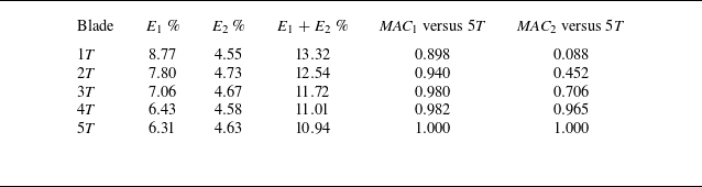
Table 3. Long description
A table comparing blade pressure field data across different modes and record lengths. The table has six rows and six columns. Column headers are Blade, E1 percent, E2 percent, E1 plus E2 percent, MAC1 versus 5T, and MAC2 versus 5T. Row labels are 1T, 2T, 3T, 4T, and 5T. Row 1: 1T, 8.77, 4.55, 13.32, 0.898, 0.088. Row 2: 2T, 7.80, 4.73, 12.54, 0.940, 0.452. Row 3: 3T, 7.06, 4.67, 11.72, 0.980, 0.706. Row 4: 4T, 6.43, 4.58, 11.01, 0.982, 0.965. Row 5: 5T, 6.31, 4.63, 10.94, 1.000, 1.000.
The POD modal-energy content and record-length sensitivity for the tower pressure field.
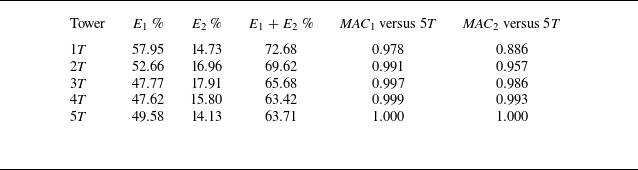
Table 4. Long description
A table with five rows and six columns comparing modal energy content and record-length sensitivity for tower pressure fields. The columns are labeled Tower, E1 percent, E2 percent, E1 + E2 percent, MAC1 versus 5T, and MAC2 versus 5T. The rows are labeled with different tower configurations: 1T, 2T, 3T, 4T, and 5T. Each row provides specific values for the modal energy fractions and modal assurance criterion coefficients. Row 1T: 57.95, 14.73, 72.68, 0.978, 0.886. Row 2T: 52.66, 16.96, 69.62, 0.991, 0.957. Row 3T: 47.77, 17.91, 65.68, 0.997, 0.986. Row 4T: 47.62, 15.80, 63.42, 0.999, 0.993. Row 5T: 49.58, 14.13, 63.71, 1.000, 1.000.
Pressure-POD modal-energy spectra and cumulative energy curves for the blade and tower surfaces, comparing cumulative
 $1T$
with
 $5T$
records.

For the blade pressure field, the first two modes contain a relatively small fraction of the total pressure-fluctuation energy. Over the full
 $5T$
record, the first and second modes account for
 $E_1=6.31\,\%$
and
 $E_2=4.63\,\%$
, respectively, with a cumulative contribution
 $E_1+E_2=10.94\,\%$
. This confirms that the blade pressure field is characterized by a broad modal-energy distribution. The first blade mode is reasonably stable with record length, reaching
 ${\textit{MAC}}_1=0.980$
already at
 $3T$
. Conversely, the second mode is more sensitive to the sampling window:
 ${\textit{MAC}}_2=0.706$
at
 $3T$
, but increases to
 ${\textit{MAC}}_2=0.965$
at
 $4T$
.
For the tower pressure field, the modal-energy distribution is much more concentrated in the leading modes. In the
 $5T$
record, the first two modes account for
 $E_1=49.58\,\%$
and
 $E_2=14.13\,\%$
, corresponding to a cumulative energy fraction of
 $63.71\,\%$
. The tower modes are also highly robust with respect to record length: already at
 $3T$
, the modal assurance criterion values with respect to the
 $5T$
modes are
 ${\textit{MAC}}_1=0.997$
and
 ${\textit{MAC}}_2=0.986$
.


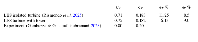
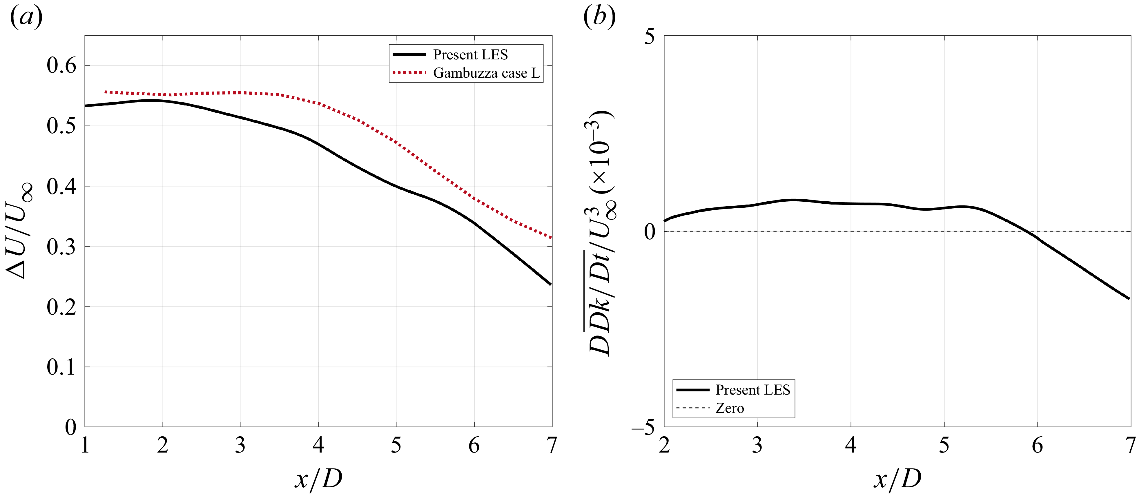

 t/T
 f/fT
 fT

 t/T
 f/fT
 fT
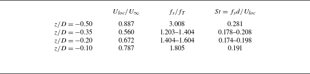

 y
 U∞/R
 QD2/U∞2=126
 U∞2

 U∞
 y
 U∞/R
 U∞2

 U∞
 R
 x/D=0.2
 0.4
 1.0
 2.0
 4.0

 z/D=−0.25
 z/D=0.25
 U∞
 y
 U∞/R
 U∞2

 ρ0U∞2

 ρU∞2


 Ω2

 x/D=0.0;1.0;2.0
 y/D=2.0;4.0;8.0
 z/D=2.0;4.0;8.0

 R|T|
 x/D=1,z/D=0.5

 x/D=0.0;1.0;2.0
 y/D=2.0;4.0;8.0
 z/D=2.0;4.0;8.0

 p^\em rms′
 10D
 x−y
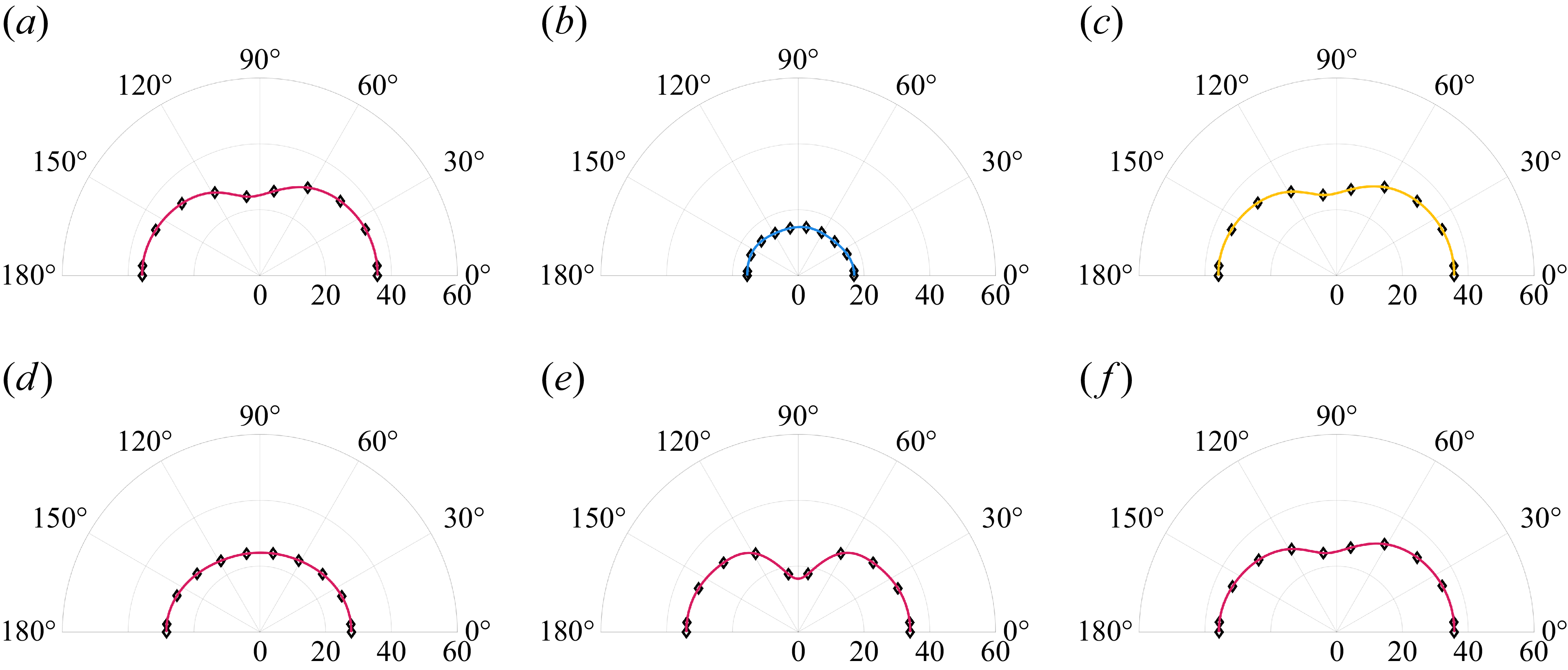
 p^\em rms′
 10D
 y−z

 p^\em rms′
 y
 z

 p^\em rms′
 10D
 x−y
 y−z
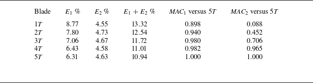
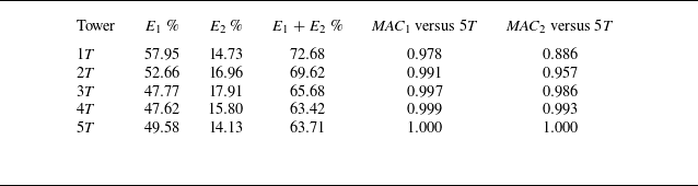

 1T
 5T


 Open access

