2. Experimental set-up

The current cross-wire measurements were conducted in the high-Reynolds-number boundary layer wind tunnel (HRNBLWT), located at the University of Melbourne. This facility is designed for studying high-$Re$ turbulent boundary layers, while also ensuring relatively low free stream turbulence intensity levels where $\sqrt {\overline {u^2}}/U_\infty < 0.05$ – $0.2\,\%$ depending on the streamwise location (Nickels et al. Reference Nickels, Marusic, Hafez and Chong2005; Marusic et al. Reference Marusic, Chauhan, Kulandaivelu and Hutchins2015). The measurements are taken at three different $x$ locations – $2$, $7$ and $18\ {\mathrm {m}}$ downstream of the tripped inlet to the working section. For the first set of measurements, the free stream velocity ($U_\infty$) is fixed at $15\ \mathrm {m\ s}^{-1}$, while the streamwise position is varied. Since the friction velocity is only weakly dependent on the streamwise distance (for a fixed free stream velocity), this allows measurements at different $Re$ using the same probe while still ensuring that our viscous-scaled sensor size is relatively constant. In addition to the matched spatial resolution measurements, we extend the $Re$ range by measuring at $U_\infty \approx 30\ \mathrm {m\ s}^{-1}$ and $x \approx 18$ m using the same cross-wire probe. Consequently, the viscous length scales are now smaller and thus the spatial resolution is poorer relative to the $15\ \mathrm {m\ s}^{-1}$ cases. However, the large-scale contributions which are several orders of magnitude larger than the sensor size remain unaffected, and therefore the dataset provides useful $Re$ trends for these scales.

The details of the cross-wire experimental conditions (solid symbols) are summarised in table 1. Here, we employ the coordinate system $x$, $y$ and $z$ to refer to the streamwise, spanwise and wall-normal directions, respectively, and $u$, $v$ and $w$ the corresponding fluctuating velocities. The superscript ‘$+$’ denotes viscous scaling of length (e.g. $z^+=zU_\tau /\nu$), velocity (e.g. $U^+=U/U_\tau$) and time (e.g. $t^+=tU_\tau ^2/\nu$), where $U_\tau$ and $\nu$ are the mean friction velocity and the kinematic viscosity of the fluid, respectively. Capitalisation (e.g. $U$) and overbar (e.g. $\overline {u^2}$) indicate time-averaged quantities. The symbols $\bullet$, $\blacksquare$ and $\blacklozenge$ in table 1 denote the cases where spatial resolution is maintained constant, while the highest $Re$ case ($\blacktriangle$) yields a relatively poorer spatial resolution. The value for friction velocity, $U_\tau$, and boundary layer thickness, $\delta$, given in table 1 have been obtained by fitting the mean velocity profile to a composite velocity formulation of Chauhan, Monkewitz & Nagib (Reference Chauhan, Monkewitz and Nagib2009). The sampling interval $\Delta t$ is chosen so that it is sufficiently low, to capture the smallest energetic length scale (i.e. $\Delta t^+ < 3$, Hutchins et al. (Reference Hutchins, Nickels, Marusic and Chong2009)), while the total sampling time $T$ corresponds to approximately 20 000 boundary layer turnover times ($TU_\infty /\delta$).

Table 1.

Experimental parameters for the cross-wire measurements (solid symbols), configured to measure the streamwise and spanwise velocities. Also shown are the experimental parameters for the atmospheric surface-layer dataset () from Hutchins et al. (Reference Hutchins, Chauhan, Marusic, Monty and Klewicki2012). Here $\Delta t$ and $T$ denote the sampling interval and the total sampling time, respectively.

Figure 1 shows the custom cross-wire probe used, where dimensions occupied by $2.5\ \mathrm {\mu }\textrm {m}$ diameter platinum hot-wire sensors are $0.4\times 0.4$ mm ($l_x \times l_y$) in the $x$ and $y$ directions with a separation of 0.2 mm ($\Delta s_z$) in the $z$ direction. The hot-wire prongs are stainless steel wires of diameter $250\ \mathrm {\mu }\textrm {m}$, ground down to a tip diameter of $20\ \mathrm {\mu }\textrm {m}$, which are then inserted into specially designed ceramic holders. The prongs are copper plated before the platinum wires are soldered to them. An important feature of these prongs is that, although the whole probe body is tilted at approximately $10^\circ$ towards the wall (to access near-wall velocity statistics), the hot-wires themselves are kept parallel to the wall. This feature, which unfortunately is not available in commercial probes, is essential in minimising errors arising from an inclination of the cross-wire sensor plane with respect to the wall. For example, Baidya et al. (Reference Baidya, Philip, Hutchins, Monty and Marusic2019a) showed that the inclined sensor plane cannot be fully accounted for through a typical calibration procedure, where contributions from the out-of-plane velocity are ignored. The inclined sensor plane results in increased sensitivity to the out-of-plane velocity component, leading to a large error of up to 10 % for the turbulent stresses in the log region. In addition, the custom probe allowed us to incorporate key design information provided from probe simulations into the design. That is, the custom probe is designed such that the wire separation distance is smaller than the wire length dimensions (see figure 1) since it is found that the former dominates the errors when measuring $v$ (Philip et al. Reference Philip, Baidya, Hutchins, Monty and Marusic2013b).

Figure 1.

Schematic of a cross-wire probe configured to measure the streamwise and spanwise velocities. The red and blue wires are located on their respective coloured planes. $l$ and $\Delta s_z$ denote the sensor length and the spacing between the sensors (in the wall-normal direction), respectively.

The hot-wires are operated in constant temperature mode with an overheat ratio of 1.8, while a full two-dimensional calibration of the cross-wire probe is performed in situ using a calibration jet facility that rotates the jet about the wall-normal axis of the cross-wire sensors (for details, see Morrill-Winter et al. (Reference Morrill-Winter, Klewicki, Baidya and Marusic2015)). During the two-dimensional calibration, the voltages from the two sensors are recorded at 12 to 17 different velocities across 0–1.1 $U_\infty$ and 11 jet angles spanning ${\pm }30^\circ$ about the $z$ axis to build up a voltage-to-velocity conversion map. Figure 2(a) shows voltage pairs ($E_1,E_2$) obtained for multiple jet velocity and angle combinations during a typical two-dimensional calibration. In order to ensure a smooth voltage-to-velocity conversion map, the recorded voltages are fitted to a functional form. The functional form utilised for the current study prescribes (i) a collapse of hot-wire voltages curves as a function of effective velocity occurs across all jet angles (Browne, Antonia & Shah Reference Browne, Antonia and Shah1988) and (ii) the response of the hot-wire to the flow angles follows a sinusoidal function (Hinze Reference Hinze1975; Morrill-Winter et al. Reference Morrill-Winter, Klewicki, Baidya and Marusic2015). Third-order polynomials are used to describe the effective velocities as functions of the hot-wire voltages. Prescribing (i) and (ii), and assuming that the inclination angle of the two hot-wires are at ${\pm }45^\circ$ with respect to the $x$ direction (the cross-wire probes used in the experiments were designed such that the hot-wires are at ${\pm }45^\circ$) results in

(2.1a,b)\begin{equation} \left.\begin{gathered} \frac{U_{{eff}1}^2}{U_{{jet}}^2} = \cos^2\left(\gamma + \frac{\rm \pi}{4}\right) + k^2\sin^2\left(\gamma + \frac{\rm \pi}{4}\right) \\ \text{and}\\ \frac{U_{{eff}2}^2}{U_{{jet}}^2} = \cos^2\left(\gamma - \frac{\rm \pi}{4}\right) + k^2\sin^2\left(\gamma - \frac{\rm \pi}{4}\right), \end{gathered}\right\}\end{equation}

where $U_{{eff}1}$ and $U_{{eff}2}$ are effective velocities from the two hot-wires, $U_{{jet}}$ and $\gamma$ are, respectively, the jet velocity and angle with respect to the cross-wire probe and $k$ is the axial sensitivity coefficient which usually varies from 0 to 0.2 (Champagne, Sleicher & Wehrmann Reference Champagne, Sleicher and Wehrmann1967). Following algebraic and trigonometric manipulations (2.1) leads to $U_{{eff}1}^2 + U_{{eff}2}^2 = U_{{jet}}^2(1+k^2)$, which corresponds to an equation for a circle. Figure 2(b) shows the effective velocities from the two-dimensional calibration shown in figure 2(a), where an equation for a circle provides a good description of the calibration points, particularly at higher jet velocities. Note that the effective velocities in figure 2(b) are shown normalised by the effective velocity at $\gamma = 0$, which is a constant factor of $U_{jet}$ according to (2.1). At low velocities, the heat transferred from the hot-wire is no longer dominated by the forced convection (Collis & Williams Reference Collis and Williams1959; Hatton, James & Swire Reference Hatton, James and Swire1970), presumably resulting in the departure from (2.1) observed in figure 2(b). In addition to the jet calibration, the calibration corresponding to zero jet angle is repeated in the wind tunnel. Thus, for a case when no misalignment exists between the calibration jet and the wind tunnel, the two calibration curves should be identical. However, in practice, a non-zero misalignment exists and the in-plane misalignment angle (the sensor plane is parallel to the $x$–$y$ plane in the current study) can be determined such that the disparity between the hot-wire voltages at the zero jet angle after accounting for the misalignment and the wind tunnel calibration is minimised. It should be noted that, since the in-plane misalignment is the leading-order contributor to the error in the evaluated velocity (Baidya et al. Reference Baidya, Philip, Hutchins, Monty and Marusic2019a), the influence of the out-of-plane misalignment is ignored for the current misalignment correction procedure. Here $U$ and $V$ are calculated from the corrected jet angle and jet velocity to create a voltage–velocity lookup table, and the recorded voltages during the course of profiling are linearly interpolated based on the lookup table to convert to velocities. In addition, the test-section temperature increased more severely for the $30\ \mathrm {m\ s}^{-1}$ dataset compared with the $15\ \mathrm {m\ s}^{-1}$ cases. This meant that the difference in the ambient temperature during the two-dimensional calibration and the experiment was more pronounced for the $30\ \mathrm {m\ s}^{-1}$ dataset. Hence, the hot-wire voltages for the $30\ \mathrm {m\ s}^{-1}$ experiments were offset by values $(\Delta E_1, \Delta E_2)$ such that the compensated $U$ profile agreed with the single-normal hot-wire measurements. Note that the offset voltages $\Delta E_1$ and $\Delta E_2$ are functions of $z$, and correspond to the change in the hot-wire voltages due to different ambient conditions.

Figure 2.

(a) Hotwire voltage ($E_1,E_2$) and (b) effective velocity ($U_{{eff}1},U_{{eff}2}$) pairs from a typical two-dimensional cross-wire calibration. (a) Constant jet velocity ($U_{{jet}}$) and jet angle ($\gamma$) lines determined from calibration points are indicated as solid (—) and dotted ($\boldsymbol {\cdot }\boldsymbol {\cdot }\boldsymbol {\cdot }$) lines. (b) The effective velocities at a constant jet velocity are shown normalised by the value at the zero jet angle, while a fitted circle is shown as a dashed line (- - -). The $\circ$ symbols showing the calibration points in panels (a,b) are coloured according to the jet velocities.

The final dataset considered are measurements from the atmospheric surface layer, obtained utilising three-component sonic anemometers (Campbell Scientific CSAT3), from Hutchins et al. (Reference Hutchins, Chauhan, Marusic, Monty and Klewicki2012). The surface layer experiments allow access to very high $Re$, which is difficult to achieve in the laboratory, allowing the assessment of $Re$ trends to be extended to $Re_\tau \equiv U_\tau \delta /\nu \sim O(10^6)$. The dataset presented here (denoted using symbol ) corresponds to an hour of measurement, carefully selected from nine days of available measurements based on the requirement of near-neutral stability, appropriate incoming flow direction relative to the sonic anemometer and steady wind (see Hutchins et al. (Reference Hutchins, Chauhan, Marusic, Monty and Klewicki2012), for full details of data selection criteria). Velocity measurements from nine sonic anemometers logarithmically spaced from $z = 1.42\ \textrm {m}$ to 25.69 m on a vertical tower are considered here. The corresponding friction-based Reynolds number is estimated to be $Re_\tau \approx 7.2 \times 10^5$, where $U_\tau$ is calculated under the assumption that the viscous scaled Reynolds shear stress peaks at unity, while $\delta$ is inferred based on turbulent stress profiles and two-point correlations.

3. Moments of the spanwise velocity

Figures 3(a) and 3(b) show the second moment (variance) of the spanwise velocity, $\overline {v^2}$, where the wall distance is normalised with viscous and outer units, respectively. The vertical error bars denote uncertainty levels in $\overline {v^2}$, estimated as ${\pm } 5\,\%$ for the lower $Re$ laboratory data ($Re_\tau \approx 2500$–10 000) and ${\pm }10\,\%$ for the $Re_\tau \approx 18\,000$ dataset. These error bars are estimated based on cross-wire probe uncertainty analysis (Baidya et al. Reference Baidya, Philip, Hutchins, Monty and Marusic2019a), uncertainty in determining the friction velocity (Winter Reference Winter1979; Klewicki et al. Reference Klewicki, Saric, Marusic and Eaton2007) and the spread in statistics observed during experiment repeats. The peak $\overline {v^2}^+$ occurs at $z^+ \approx 50$, which is farther away from the wall than the $\overline {u^2}^+$ peak location at $z^+ \approx 15$ (Sillero et al. Reference Sillero, Jiménez and Moser2013; Lee & Moser Reference Lee and Moser2015). In the log region (i.e. where the mean velocity is seen to follow a log law – shown by horizontal bars in figure 3a), $\overline {v^2}$ follows a log–linear relationship in a similar manner to the $\overline {u^2}$ statistics, given by,

(3.1)\begin{equation} \dfrac{\overline{v^{2}}}{U_\tau^2} ={-}A_{2} \ln{\dfrac{z}{\delta}} + B_{2}, \end{equation}

where $A_{2}$ and $B_{2}$ indicate the logarithmic slope and intercept of the fit, respectively. The slope of the logarithmic behaviour in figure 3 is consistent across the dataset with a matched spatial resolution ($\bullet$, $\blacksquare$, $\blacklozenge$) and with the $\overline {v^2}$ statistics from DNS (dotted and dash-dotted lines), while a shallower slope is recorded for the $Re_\tau \approx 18\,000$ dataset. This is because a lower spatial resolution sensor leads to underestimated smaller scales, causing $\overline {v^2}$ statistics to be increasingly attenuated closer to the wall (Philip et al. Reference Philip, Baidya, Hutchins, Monty and Marusic2013b). For the current experiment, the $\overline {v^2}$ errors due to the finite sensor effects become prominent below $z^+ \lesssim 100$ (indicated by a vertical dash-dotted line in figure 3a) where the biases introduced exceed the uncertainty of the experiment (which is equal to ${\pm }5$ and ${\pm }10$ % for the $U_\infty = 15$ and $30\ \mathrm {m\ s}^{-1}$ cases, respectively). The slope of the logarithmic $\overline {v^2}$ behaviour for the $Re_\tau \approx 10\,000$ dataset, based on a linear regression in the region $3\sqrt {\delta ^+} \leqslant z^+ \leqslant 0.15 \delta ^+$ (indicated by the green horizontal bar in figure 3a), provides $A_{2} \approx 0.27$. It should be noted that the lower bound selected for the log region is based on a $z$ location where the inertial forces become leading order in the mean momentum balance (Morrill-Winter, Philip & Klewicki Reference Morrill-Winter, Philip and Klewicki2017), which also coincides with an onset of a logarithmic behaviour in both the $U$ and $\overline {u^2}$ statistics (Marusic et al. Reference Marusic, Monty, Hultmark and Smits2013). Furthermore, setting $A_{2} = 0.27$, the value for $B_2$ based on the regression varies from 1.3 at $Re_\tau \approx 2500$ to 1.5 at $Re_\tau \approx 10\,000$ (only the matched spatial resolution cases are considered to isolate the $Re$ effects) as shown in figure 4. The $A_2$ and $B_2$ values from the current study are in good agreement with Zimmerman et al. (Reference Zimmerman2019), who obtained $A_2 \approx 0.26$ and $B_2 \approx 1.6$ at $Re_\tau \approx 8000$ in the same facility (the HRNBLWT) with a different probe. Here, the $A_2$ and $B_2$ values for the Zimmerman et al. (Reference Zimmerman2019) data have been re-evaluated, based on the definition for the log region and $\delta$ that is consistent with the current study. Hence, the value of $B_2$ differs slightly from that given in Zimmerman et al. (Reference Zimmerman2019), where the boundary layer thickness is taken to be the $z$ location where $U = 0.99U_\infty$. Note that, Zimmerman et al. (Reference Zimmerman2019) obtain a somewhat different value of $A_2\approx 0.34$, when they measure in the Flow Physics Facility. However, this difference is presumed to be due to an underdeveloped wake found in the Flow Physics Facility, where the velocity profile beyond $z/\delta \geqslant 0.8$ is found to deviate from the canonical profile (Zimmerman et al. Reference Zimmerman2019).

Figure 3.

Variance of the spanwise velocity, $\overline {v^2}$, shown in (a) viscous and (b) outer normalisations. The solid symbols ($\bullet$, $\blacksquare$, $\blacklozenge$, $\blacktriangle$) correspond to measurements conducted at HRNBLWT, while the empty symbol () is an atmospheric surface layer dataset obtained using a sonic anemometer, from Hutchins et al. (Reference Hutchins, Chauhan, Marusic, Monty and Klewicki2012). The dotted and dash-dotted lines are $\overline {v^2}$ statistics from the DNS database of Schlatter & Örlü (Reference Schlatter and Örlü2010) and Sillero et al. (Reference Sillero, Jiménez and Moser2013), respectively. (a) The vertical dotted and dash-dotted line correspond to $z^+ = 50$ and $z^+ \approx 100$, respectively, while the dashed lines show log–linear relations with the slope $A_2 = 0.27$. Furthermore, the horizontal bars, coloured according to the corresponding $Re$, denote the location of the log region ($3\sqrt {\delta ^+} \leqslant z^+ \leqslant 0.15\delta ^+$).

Figure 4.

The logarithmic intercept, $B_2$, for the $\overline {v^2}$ statistics as a function of $Re_\tau$. The magenta symbol, $\blacktriangleright$, corresponds to measurements by Zimmerman et al. (Reference Zimmerman2019) (where the $B_2$ value has been recomputed utilising a consistent definition for the log region and $\delta$ as the current study).

Also shown in figure 3 are the $\overline {v^2}$ statistics measured in the atmospheric surface layer by Hutchins et al. (Reference Hutchins, Chauhan, Marusic, Monty and Klewicki2012), and denoted by . These field measurements have larger uncertainties (the error bars reflect ${\pm }10 \,\%$ uncertainty in the friction velocity due to the assumption that $-\overline {uw}^+$ peaks at unity) compared with the laboratory measurements. Although the large uncertainty means that a wide range of $A_2$ is permissible to describe the log–linear $\overline {v^2}$ behaviour, $A_2 = 0.27$ is nevertheless consistent with the measurements (see dashed lines, figure 3a).

In the context of AEH, an increase in $Re$ is reflected by a larger number of self-similar hierarchy levels required to model the wall-bounded flow. Thus, since the $u$ and $v$ contributions from each hierarchy level are additive, $\overline {u^2}^+$ and $\overline {v^2}^+$ at a fixed $z^+$ increases proportionally with the number of hierarchy levels, which scales as $\log {\delta ^+}$ (Perry & Chong Reference Perry and Chong1982). Indeed, an increase in $\overline {v^2}^+$ at a fixed $z^+$ location is observed in the current experiments (see figure 3a). Notably, the slope of logarithmic $\overline {v^2}$ ($A_2 \approx 0.27$) is shallower than that found in $\overline {u^2}$, where $A_{1} \approx 1.2$ (Marusic et al. Reference Marusic, Monty, Hultmark and Smits2013). If one accepts the AEH description, a possible explanation for the difference in the slope between the $\overline {u^2}$ and $\overline {v^2}$ behaviour is that the wall-bounded flow is better represented by a hierarchy of multiple streamwise aligned eddies travelling in a packet (Adrian, Meinhart & Tomkins Reference Adrian, Meinhart and Tomkins2000), rather than a hierarchy of single isolated eddies where the logarithmic slopes observed for $\overline {u^2}$ and $\overline {v^2}$ are similar (i.e. $A_{1} \approx A_{2}$). The streamwise aligned eddies lead to a strengthening of the $u$ contributions per hierarchy level, while the $v$ contributions remain relatively unaffected, leading to $A_{1} > A_{2}$, which is more consistent with the experimental data (Baidya et al. Reference Baidya, Philip, Monty, Hutchins and Marusic2014).

In the asymptotic limit, AEH predicts that $B_2$ will reach a constant, in a similar manner to the $\overline {u^2}$ behaviour, where the logarithmic intercept, $B_1$, also approaches a constant. While the empirical evidence supports $B_1$ approaching a constant at sufficiently high $Re$ (Marusic, Uddin & Perry Reference Marusic, Uddin and Perry1997; Marusic et al. Reference Marusic, Monty, Hultmark and Smits2013), an increase in $B_2$ is observed for the current dataset with increasing $Re$, as shown in figure 4 on log–linear axes. Furthermore, the atmospheric surface layer measurement suggests that $B_2$ might maintain a $\log \delta ^+$ behaviour despite an increase in $Re$ by over an order of magnitude. We note that, it is difficult to draw a robust conclusion on $Re$-dependency of $B_2$ based on figure 4 and further high quality $\overline {v^2}$ measurements in the $Re_\tau \sim 10^4$–$10^6$ range are necessary to make a more definitive conclusion. A discrepancy between the AEH predictions and the experimental results is also observed in terms of the spanwise velocity tendency to exhibit extreme values compared with a Gaussian distribution. That is, the $v$ flatness values exceed 3 (super-Gaussian behaviour) in the log region (e.g. Fernholz & Finley (Reference Fernholz and Finley1996), and this is consistent with our observations too, but not shown here for brevity) while a value lower than 3 (sub-Gaussian behaviour) is predicted by AEH (Woodcock & Marusic Reference Woodcock and Marusic2015). This is in contrast to the $u$ signal, which exhibits sub-Gaussian behaviour as predicted by AEH. Consequently, the higher-order even moments of $u$ and $v$ also behave differently – e.g. the logarithmic slope for the higher-order moments increasingly deviate away from a Gaussian behaviour in the opposite direction (Meneveau & Marusic Reference Meneveau and Marusic2013; Yang et al. Reference Yang, Baidya, Lv and Marusic2018). The discrepancy between the experiment and AEH predictions is thought to arise due to a degree of correlation being retained among eddies of different scales in a real flow (Meneveau & Marusic Reference Meneveau and Marusic2013). For example, de Silva et al. (Reference de Silva, Woodcock, Hutchins and Marusic2016) showed that an introduction of a slight non-randomness in AEH hierarchy, whereby a restriction is imposed on the placement of eddies such that a minimum separation is maintained (i.e. two eddies from the same hierarchy level cannot coexist at the same location), results in a $u$ and $v$ behaviour that is more consistent with the experiments.

4. Energy spectral density

Figure 5 shows the energy spectral density of $v$ as a function of streamwise wavelength, $\lambda _x$, at selected $z$ locations for the $Re_\tau \approx 10\,000$ case. The premultiplied energy spectra of spanwise velocity fluctuations, $k_x\phi _{vv}$, provide a measure of $\overline {v^2}$ contributions for a given streamwise length scale, since $\int _0^\infty k_x \phi _{vv}\, \mathrm {d}\ln {k_x} = \overline {v^2}$, where $k_x$ corresponds to the streamwise wavenumber (i.e. $\lambda _x = 2{\rm \pi} /k_x$). Note that, the energy spectral density, $\phi _{vv}$, is a function of $k_x$ (or $\lambda _x$) and therefore is distinct from (but related to) the spectral density per unit non-dimensional wavenumber $k_x\mathcal {L}$, $\varPhi _{vv}(k_x \mathcal {L})$, where $\mathcal {L}$ is some length scale of interest (for further details see Nickels & Marusic (Reference Nickels and Marusic2001)), used by Perry & Chong (Reference Perry and Chong1982) and in the subsequent works.

Figure 5.

Premultiplied energy spectra of $v$ fluctuations for a $Re_\tau \approx 10\,000$ turbulent boundary layer. The $v$ spectra shown correspond to the wall heights $z^+ = 50$ ($\blacktriangleleft$), $z^+ = 3 \sqrt {\delta ^+}$ ($\bullet$), $z = 0.15\delta$ ($\blacktriangleright$) and $z=0.6\delta$ ($\blacksquare$), as indicated in figure 6(c).

It is evident from figure 5 that within the log region the most energetic wavelength becomes longer with wall distance (e.g. $\bullet$ and $\blacktriangleright$), while in the outer layer it remains relatively fixed at $\lambda _x \approx \delta$ (e.g. $\blacktriangleright$ and $\blacksquare$). It should be noted that the temporal hot-wire signals have been converted to the spatial domain by invoking Taylor's frozen turbulence hypothesis (Taylor Reference Taylor1938), where the turbulent motions at all length scales are assumed to convect at the local mean velocity, $U(z)$. However, it is known that the convection velocity is scale-dependent (del Álamo & Jiménez Reference del Álamo and Jiménez2009; Monty & Chong Reference Monty and Chong2009); hence, we expect a slight change in the actual shape of the $v$ spectrum following this procedure. Although we cannot entirely rule out its influence here, we expect the redistribution of energy beyond the log region ($z^+ \geqslant 3 \sqrt {\delta ^+}$, see vertical dashed lines in figure 6) to correspond to a small fraction of the overall energy, as at these $z$ locations the convection velocity across the scales become more uniform (del Álamo & Jiménez Reference del Álamo and Jiménez2009).

Figure 6.

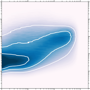
Premultiplied energy spectrogram of $v$ fluctuations as a function of wall height, $z$, and wavelength, $\lambda _x$, at (a) $Re_\tau \approx 2500$, (b) $Re_\tau \approx 5000$ and (c) $Re_\tau \approx 10\,000$. The vertical dashed lines indicate the bounds of the log region, which are taken here to be $z^+ = 3\sqrt {\delta ^+}$ and $z/\delta = 0.15$, while the black dashed lines show the location of the energetic ridge identified. The solid white lines correspond to contour levels 0.2, 0.4 and 0.6. Here ‘FP’ denotes the location of the energetic ‘footprint’ from the very large-scale structure. The wavelengths corresponding to small-, intermediate- and large-scales are denoted by $SS, IS\ {\rm and}\ LS$, respectively.

Figure 6(a–c) display the full map of the $v$-spectrogram at various $Re$, where the colours indicate the energetic content at a particular wall height and wavelength. Hence, the $v$ spectra shown in figure 5 correspond to $k_x\phi _{vv}$ along the vertical lines in figure 6(c) with a matched symbol. Unlike the $u$-spectrogram (e.g. Hutchins & Marusic (Reference Hutchins and Marusic2007a) and also figure 12(a) in appendix A) there is no apparent inner/outer site separation even at the highest $Re$ data. Rather, it appears that for $z^+<70$, there exists a ridge of energy at a fixed streamwise wavelength $\lambda _x^+\approx 350$. Through the log region, there are clear signs of energy scaling with distance from the wall, with the energetic ridge seeming to follow the line $\lambda _x=5z$ for $70\leqslant z^+ \leqslant 0.15\delta ^+$. Moreover, in the wake region, the energy seems to reach a ridge at a constant $\lambda _x/\delta \approx 0.75$. The energetic ridge, adhering to these trends, is indicated by the black dashed lines in figure 6. The distribution of the energetic $u$ content relative to the location of the black dashed line in figure 12(a) of appendix A, indicates that the $u$ fluctuations are dominated by energetic scales that are at a longer streamwise wavelength than the $v$ fluctuations. This is due to the tendency of $u$ fluctuations to align in the streamwise direction, while the spanwise velocity regions remain isolated (Sillero, Jiménez & Moser Reference Sillero, Jiménez and Moser2014).

Figure 6(a–c) also indicate that the small-scale, near-wall $v$ spectral content is invariant with Reynolds number when scaled in viscous units. Note that, although the effects from finite sensor dimensions (the $v$ spectra closely follow the $w$ spectra behaviour described in Baidya et al. (Reference Baidya, Philip, Hutchins, Monty and Marusic2019b)) become more severe in the near-wall region, we expect this effect to remain constant across figure 6(a–c) since we have maintained a matched spatial resolution (Philip et al. Reference Philip, Baidya, Hutchins, Monty and Marusic2013b; Baidya et al. Reference Baidya, Philip, Hutchins, Monty and Marusic2019b). Similarly, even though the assumption that the convection velocity for Taylor's hypothesis is equal to the local mean velocity is less valid in the near-wall region (del Álamo & Jiménez Reference del Álamo and Jiménez2009), the redistribution of the energetic content in the $v$-spectrogram is expected to be similar across the three $Re$ cases. In contrast to the invariance of the near-wall $v$-spectrogram when $\lambda _x^+ \lesssim 1000$, the contours outside this region shift towards higher $\lambda _x^+$ with increasing $Re$. This is likely because, in a similar manner to the streamwise velocity (e.g. Hutchins & Marusic (Reference Hutchins and Marusic2007a), and also figure 12(a), in appendix A) the influence of the very large-scale features that reside in the log region extends to the wall for the spanwise velocity. Thus, the very large-scale feature has a footprint that extends to the wall, leading to large-scale energetic content in $v$ at $z^+\sim 10$ and $\lambda /\delta \sim 1$ (this location is indicated by ‘FP’) as shown in figure 6. Note that, although the presence of the large-scale footprint at the wall leads to small-scales that are more strongly modulated with the large-scale $u$ at high $Re$ (Mathis, Hutchins & Marusic Reference Mathis, Hutchins and Marusic2009; Talluru et al. Reference Talluru, Baidya, Hutchins and Marusic2014), the small-scale energetic content seems to be preserved on the time-averaged sense, and therefore exhibits Reynolds number invariance when scaled in viscous units. Notably, the energetic footprint is absent from the $w$-spectrogram and the Reynolds shear stress cospectrogram (as shown by Baidya et al. (Reference Baidya, Philip, Hutchins, Monty and Marusic2017), and reproduced in figure 12b,c), due to the impermeability condition at the wall, which restricts large-scale wall-normal fluctuations in this region (Perry & Chong Reference Perry and Chong1982). Furthermore, in an analogous manner to the classical mean flow theory (e.g. Millikan Reference Millikan1938), the peak contribution in the $v$-spectrogram and the $uw$-cospectrogram (and to a lesser extent $w$-spectrogram) follow a viscous and $\delta$ scaling in the near-wall and outer part of the boundary layer, respectively, while a transition from these two regimes occurs in the log region where the dominant modes scale with $z$.

Figure 7(a,b) show the influence of the Reynolds number on the $v$ energetic content at the near-wall ($z^+ = 50$) and log ($z^+ = 3 \sqrt {\delta ^+} \approx 310$ at $Re_\tau \approx 10\,000$) regions, respectively. Here, the vertical dotted line indicates the spectral cutoff limit for the small-scale contribution (the choice for the cutoff wavelength is detailed in § 4.1). The small-scale spectral-cutoff also corresponds to the lower horizontal dotted lines in figure 6(a–c). Thus, the intermediate- and large-scale $v$ fluctuations, where $\lambda _x$ exceeds the cutoff value (the intermediate- and large-scales are distinguished in § 4.1), are responsible for an increase in the peak $\overline {v^2}$ observed at $z^+ = 50$ as a function of $Re$. Note that, due to poorer spatial resolution, the small-scale energetic content is not as well-resolved for the $Re_\tau \approx 18\,000$ dataset as the other three cases, and therefore this part of the spectrum is not shown in figure 7. The increase in the combined contribution from the intermediate- and large-scales to the broadband $\overline {v^2}$ observed in the near-wall region at high $Re$ may provide clues on the scalability of the flow control strategies, which introduce oscillation or travelling waves at the wall to alter the near-wall $v$ (Choi, Moin & Kim Reference Choi, Moin and Kim1994; Quadrio Reference Quadrio2011). These strategies achieve drag reduction by suppressing the near-wall streaks (Karniadakis & Choi Reference Karniadakis and Choi2003; Quadrio Reference Quadrio2011), which are increasingly modified by the intermediate- and large-scale contributions at high $Re$ (Hutchins & Marusic Reference Hutchins and Marusic2007b; Talluru et al. Reference Talluru, Baidya, Hutchins and Marusic2014); providing an additional mechanism that may explain the reduced drag performance observed with increasing $Re$ (Hurst, Yang & Chung Reference Hurst, Yang and Chung2014; Gatti & Quadrio Reference Gatti and Quadrio2016).

Figure 7.

Premultiplied $v$ spectra at (a) near-wall ($z^+ = 50$) and (b) log ($z^+ = 310$) regions. The symbols $\bullet$, $\blacksquare$, $\blacklozenge$, $\blacktriangle$ correspond to $Re_\tau \approx$ 2500, 5000, 10 000 and 18 000 cases, respectively.

In AEH, the logarithmic behaviour of $\overline {v^2}$ is associated with a $\phi _{vv} \sim k_x^{-1}$ behaviour (as with $u$) when a sufficient scale separation exists between the viscous and inertial scales (Perry, Henbest & Chong Reference Perry, Henbest and Chong1986). However, no distinct plateau region, spanning across an increasingly wide range of scales at higher $Re$ (as envisioned by Perry et al. Reference Perry, Henbest and Chong1986) exists in figure 7(b). Hence, even though $\phi _{vv}$ shows clear signs of energy scaling with $z$ in the log region, there is no evidence of $\phi _{vv} \sim k_x^{-1}$ behaviour for our experiment. Instead, a peak in energetic contribution occurs at $\lambda _x^+ \approx 1100$ and a shallower departure from the maxima occurs at higher $Re$ for $\lambda _x^+ \gtrsim 1100$ (contributions below $\lambda _x^+ \lesssim 1100$ are Reynolds number invariant). Thus, the slope of the departure may eventually approach zero at sufficiently high $Re$ ($Re_\tau \gg O(10^4)$), transforming the peak into a plateau. Note that, a self-similar hierarchy of eddies do not necessarily guarantee a $k_x^{-1}$ behaviour, such as for a case when insufficient scale separation exists between the smallest and largest hierarchy levels (Davidson, Nickels & Krogstad Reference Davidson, Nickels and Krogstad2006; Baidya et al. Reference Baidya, Philip, Hutchins, Monty and Marusic2017). Nevertheless, the $Re$ trend observed in figure 7(b) is consistent with the AEH calculations for these limited scale separation cases, where an increasingly plateau-like behaviour occurs when the scale separation is increased.

4.1. Scale-decomposed $\overline {v^2}$ contributions

To further quantify how the $v$-spectrogram behaviour changes with $Re$, we will divide the $k_x\phi _{vv}$ contribution into the small, intermediate and large wavelengths, using cutoff values (denoted by the horizontal lines) as illustrated in figure 6. Since small-scale energy scales with viscous units, the limit $\lambda _{c1}$ is set in this inner-normalisation. Meanwhile, the large-scale energy scales with the outer scale, and therefore $\lambda _{c2}$ is set to be a constant fraction of $\delta$. This grouping implies that the separating thresholds ($\lambda _{c1}$ and $\lambda _{c2}$) will move apart as $Re$ (i.e. scale separation) increases. Therefore, the range of scales that will be grouped within the ‘intermediate’ range grows with $Re$.

The three regions in the $v$-spectrogram are integrated with respect to $\lambda _x$, and hence $\overline {v^2}$ can be decomposed based on the small- ($\overline {v^2}_{SS}$), intermediate- ($\overline {v^2}_{IS}$) and large-scale ($\overline {v^2}_{LS}$) contribution. That is,

(4.1)\begin{align} \overline{v^2} &= \int_{0}^{\lambda_{c1}} k_x \phi_{vv} \,\mathrm{d} \ln{\lambda_x} + \int_{\lambda_{c1}}^{\lambda_{c2}} k_x\phi_{vv} \,\mathrm{d} \ln{\lambda_x} + \int_{\lambda_{c2}}^{\infty} k_x\phi_{vv} \,\mathrm{d} \ln{\lambda_x}\nonumber\\ &= \overline{v^2}_{SS} + \overline{v^2}_{IS} + \overline{v^2}_{LS}. \end{align}

In the $v$-spectrogram, the energetic ridge at $\lambda _x^+ \approx 350$ and $\lambda _x \approx 0.75 \delta$ across a range of $z$ locations suggest that they result from viscous and $\delta$-scaled structures, respectively. Thus, to demarcate the small- and large-scale contributions, the geometric centre between these two streamwise wavelengths is selected at the lowest $Re$ ($Re_\tau \approx 2500$); therefore,

(4.2a)\begin{equation} \lambda_{c1}^+{=} \sqrt{350\times1875} = 810. \end{equation}

Furthermore, $\lambda _{c2}$ is chosen so that $\lambda _{c2} = \lambda _{c1}$ at $Re_\tau \approx 2500$, i.e.

(4.2b)\begin{equation} \lambda_{c2} = 0.32\delta. \end{equation}

Hence, the contributions from the intermediate-scales $\overline {v^2}_{IS}$ is equal to zero for the lowest $Re$ case. It should be noted that, since the turbulence is broadband, no clear boundary exists between the small-, intermediate- and large-scale contributions. Therefore, equally valid choices for the integral limits used in (4.1) could exist, different from the current definition. Note that, altering the integral limits would change the $\overline {v^2}$ contributions associated with each scale; however, the focus here is on the $Re$ trends, which remain relatively unaffected (provided that the viscous and $\delta$ scaling is used, respectively, for the integral limits $\lambda _{c1}$ and $\lambda _{c2}$).

Figure 8(a) shows that $\overline {v^2}^+_{SS}$ is invariant in the near-wall region when the spatial resolution is comparable, similar to the $\overline {u^2}$ statistics (e.g. Hutchins et al. (Reference Hutchins, Nickels, Marusic and Chong2009), and also figure 13(a) in appendix A). Furthermore, the small-scale invariance is found to be universal across all turbulent stresses, when the procedure is repeated for the other velocity components (see appendix A for further details). Hence, these $Re$ invariant contributions are likely to be associated with the buffer layer streaks (Kim, Kline & Reynolds Reference Kim, Kline and Reynolds1971) and the quasi-streamwise vortices (Jeong et al. Reference Jeong, Hussain, Schoppa and Kim1997), where the dominating contribution scales with viscous units (Jiménez & Moin Reference Jiménez and Moin1991).

Figure 8.

Scale-decomposed $\overline {v^2}$. (a–c) Small-, intermediate- and large-scale contributions as functions of $z^+$. (d) Large-scale contributions shown against $z/\delta$. The symbols denote different $Re$: $\circ$, $Re_\tau \approx 2500$; $\square$, $Re_\tau \approx 5000$; $\lozenge$, $Re_\tau \approx 10\,000$; $\vartriangle$, $Re_\tau \approx 18\,000$. The solid, chequered and open symbols correspond to the small-, intermediate- and large-scale contributions. The horizontal bars in panels (a–c) show the location of the log region and are coloured according to the corresponding $Re$, while the solid lines demonstrate log–linear relations.

As expected, a strengthening of the intermediate-scale contribution occurs in figure 8(b) as $Re$ increases, since the hierarchy of eddies contributing to $\overline {v^2}_{{IS}}$ extends with increasing $Re$. Note that the contribution at $Re_\tau \approx 2500$ to intermediate-scale is equal to zero based on (4.2). The importance of intermediate-scales becomes clear if we consider the high-$Re$ limit, where evidence suggests that the hierarchy of eddies that are sufficiently separated from the viscous and inertially dominated scales exhibit self-similarity (Hwang & Sung Reference Hwang and Sung2018; Marusic & Monty Reference Marusic and Monty2019). Furthermore, with increasing $Re$, data in figure 8(b) show logarithmic behaviour within the inertial regime, which are made evident by the grey solid lines. This feature of the intermediate-scale would be employed later in § 4.2 (and figure 11) to construct a model for $\overline {v^2}$ in the high-$Re$ limit.

Figure 8(d) shows the large-scale contributions to $\overline {v^2}$ in outer scaling. A good collapse of $\overline {v^2}^+_{LS}$ is observed for $z/\delta > 0.5$, with a peak contribution at $z/\delta \approx 0.2$. Notably, a simple decomposition based on a spectral cutoff is more successful in demarcating the viscous and $\delta$-scaled contributions for $v$ compared with $u$. This is because the viscous and $\delta$-scaled energetic contributions are confined to a narrow wavelength band around the energetic ridge for $v$ fluctuations, whereas for the $u$-spectrogram the energetic contributions about the local peaks occur over a wider wavelength band (compare figures 6c and 12a). It should be noted that for the $Re \approx 2500$ case, a secondary peak exists in the near-wall region ($z^+ < 100$) for $\overline {v^2}_{LS}$ due to inadequate scale separation, while it is absent in the higher $Re$ cases. Thus, for the subsequent analysis this near-wall region below $z^+ < 100$ is ignored. Figure 9 shows a comparison of how the maxima in $\overline {v^2}_{LS}$ above $z^+ > 100$ varies with $Re$. Furthermore, the same procedure is applied for other turbulent stresses, where the symbols $\blacktriangledown$, $\blacksquare$ and $\bullet$ show the maxima in $\overline {u^2}_{{LS}}$, $\overline {w^2}_{{LS}}$ and $-\overline {uw}_{{LS}}$, respectively. Note that, to account for energetic contribution at larger $\lambda _x$, the streamwise cutoff wavelengths $\lambda _{c1}^+ = 2500$ and $\lambda _{c2}/\delta = 1$ are used for the streamwise velocity, while the limits given in (4.2) are maintained for demarcating the $\overline {w^2}$ and $-\overline {uw}$ stresses (see appendix A for further details). At low $Re$ ($Re_\tau \approx 2500$–5000) an increase in the peak $\overline {v^2}^+_{LS}$ contribution is observed with increasing $Re$ in a similar manner to the peak $\overline {u^2}^+_{LS}$ behaviour; however, the observed growth rate compared with $\overline {u^2}^+_{LS}$ is smaller. At increased $Re$, the data show that the maximum values deviate from the $\log {\delta ^+}$ behaviour observed at low $Re$, and the growth as a function of $Re$ is reduced. Therefore, at sufficiently high $Re$, the peak $\overline {u^2}^+_{LS}$ and $\overline {v^2}^+_{LS}$ may asymptote to constants. However, these highest Reynolds number data are the most experimentally challenging to obtain, and repeated measurements at even higher $Re$ data are required to confirm these trends. The data also suggest that the peak $\overline {w^2}^+_{LS}$ and $-\overline {uw}^+_{LS}$ exhibit $Re$ invariance at a lower $Re$ relative to the $\overline {u^2}$ and $\overline {v^2}$ stresses, as they are found to be constant across the $Re$ range examined.

Figure 9.

The $Re$ dependency of the maximum large-scale contributions in the turbulent stresses. The turbulent stress contributions are: $\blacktriangledown$, $\overline {u^2}$; $\blacktriangleleft$, $\overline {v^2}$; $\blacksquare$, $\overline {w^2}$; $\bullet$, $-\overline {uw}$. Note that the $\overline {u^2}$ contribution is shown premultiplied by a factor 0.5. The dashed line shows a $\log {\delta ^+}$ dependency.

Recent high-$Re$ measurements compiled by Marusic et al. (Reference Marusic, Monty, Hultmark and Smits2013), suggest that the slope of the logarithmic $\overline {u^2}$ behaviour is universal across pipe (internal) and boundary layer (external) flows. In contrast, a difference in the $\overline {v^2}$ slope has been noted between the internal and external flows ($A_{2} \approx 0.5$ in the channel and pipe compared with $A_{2} \approx 0.3$ in the boundary layer), albeit at a lower $Re$ (Sillero et al. Reference Sillero, Jiménez and Moser2013; Chin, Monty & Ooi Reference Chin, Monty and Ooi2014; Mehrez et al. Reference Mehrez, Philip, Yamamoto and Tsuji2019). However, at this $Re$ range, the logarithmic behaviour in $\overline {u^2}$ is also not well defined, and hence the differences in $A_{2}$ observed may simply be a low $Re$ effect. Here, we re-examine these differences by decomposing $\overline {v^2}$ based on scales at a matched $Re$, and the result is presented in figure 10. Close to the wall, the intermediate- (chequered symbols and dash-dotted lines) and large-scale (empty symbols and dashed lines) $\overline {v^2}$ contribution show good agreement between the channel and boundary layer flows, while the differences in the small-scale contributions (solid symbols and dotted lines) are likely due to differences in the spatial resolution between the boundary layer experiments and channel DNS of Lee & Moser (Reference Lee and Moser2015).

Figure 10.

(a) Comparison of scale-decomposed $\overline {v^2}$ contributions between the channel (denoted by lines, Lee & Moser Reference Lee and Moser2015) and boundary layer (symbols) flows at $Re_\tau \approx 5000$. The dotted ($\boldsymbol {\cdot }\boldsymbol {\cdot }\boldsymbol {\cdot }$), dash-dotted ($\text {-}\boldsymbol {\cdot }\text {-}$) and dashed (- - -) lines denote small-, intermediate- and large-scale contributions, respectively, while the symbols are as in figure 8. (b) The broadband $\overline {v^2}$ statistics. The vertical dashed lines in panels (a,b) denote the bounds of the log region.

In the outer region, the maximum difference in $\overline {v^2}$ occurs between the channel and boundary layer flows at $z/\delta \approx 0.33$–$0.4$, and the differences are most evident at the large scales. In the outer region, the flow is intermittent, i.e. it switches between turbulent and quiescent/non-turbulent states (Chauhan et al. Reference Chauhan, Philip, de Silva, Hutchins and Marusic2014; Kwon, Hutchins & Monty Reference Kwon, Hutchins and Monty2016). Furthermore, the quiescent core and non-turbulent regions in the channel and boundary layer flows behave differently, which is reflected in the distinct large-scale contributions observed in figure 10(a). Thus, although the logarithmic slope exhibited by the broadband $\overline {v^2}$ in the internal and external flows may appear distinct, the results suggest that the $\overline {v^2}$ contributions from the intermediate-scale wall-attached eddies may be universal between these flows. Furthermore, since the wall-attached contributions dominate the broadband $\overline {v^2}$ behaviour at high $Re$ (see § 4.2 for further details), $A_2$ values in the external and internal flow may exhibit universality at a sufficiently high $Re$.

4.2. Revisiting the $\overline {v^2}$ logarithmic behaviour

Since the sum of $\overline {v^{2}}_{{SS}}$, $\overline {v^{2}}_{{IS}}$ and $\overline {v^{2}}_{{LS}}$ returns the broadband $\overline {v^2}$, their trends in the log region can provide a better insight regarding the behaviour of the cumulative statistic, which follows (3.1) as demonstrated in § 3. Thus, here we fit functional forms to describe the small-, intermediate- and large-scale contributions and suppose that they respectively maintain the viscous, distance-from-the-wall and outer scaling to predict the $\overline {v^2}$ behaviour as a function of $Re$.

Based on an empirical observation from figure 8(a–c), log–linear functions are chosen as a first approximation to describe contributions in the log region for all three scales (it will be shown later that the resulting asymptotic prediction holds independently of the $\overline {v_{{SS}}^2}$ and $\overline {v_{{LS}}^2}$ functional forms). For the small-scale contributions, the data suggest a $\ln {z^+}$ dependence (grey solid lines) as indicated in figure 8(a). Therefore, the small-scale contributions are modelled as

(4.3)\begin{equation} \overline{v^2}_{{SS}}^+{=} -C_{{S1}} \ln z^+{+} C_{{S2}}, \end{equation}

where $C_{{S1}}$ and $C_{{S2}}$ are constants.

Meanwhile, figure 8(b) shows increasing $\overline {v^2}^+_{{IS}}$ contribution with increasing $Re$ at a fixed $z^+$. This is consistent with the eddies responsible for the intermediate-scales following the distance-from-the-wall scaling prescribed by AEH, since the self-similar attached eddy contributions from each hierarchy level are identical. This means that $\overline {v^2}$ at a particular $z^+$ location is expected to correspond to the number of contributing hierarchy levels, which exhibits a $\log {\delta ^+}$ scaling (Townsend Reference Townsend1976; Perry & Chong Reference Perry and Chong1982). Hence, based on AEH, $\overline {v^2}_{{IS}}$ is modelled to follow a $\ln {(z/\delta )}$ dependence. Hence,

(4.4)\begin{equation} \overline{v^2}_{{IS}}^+{=} \,f_{{I1}}(\delta^+)\ln{(z/\delta)} + \,f_{{I2}}(\delta^+), \end{equation}

where $f_{{I1}}$ and $f_{{I2}}$ are functions of the Reynolds number but not of $z$. Note that the $Re$ dependency prescribed for $f_{{I1}}$ and $f_{{I2}}$ is based on the logarithm slope and intercept trends observed for the fits (the logarithmic behaviour is hardly present for the $Re_\tau \approx 5000$ case) shown in figure 8(b).

The large-scale contributions, $\overline {v^2}_{{LS}}$, show a collapse as a function of $z^+$ within the log region, indicating a $\ln {z^+}$ dependence similar to the small-scale contribution, as demonstrated in figure 8(c); therefore,

(4.5)\begin{equation} \overline{v^2}_{{LS}}^+{=} \,f_{{L1}}(\delta^+)\ln z^+{+} \,f_{{L2}}(\delta^+), \end{equation}

where $f_{{L1}}$ and $f_{{L2}}$ are functions of the Reynolds number but not of $z$ as in (4.4). Here, $f_{{L1}}$ and $f_{{L2}}$ are chosen to exhibit an $Re$ dependency, since the maximum $\overline {v^2}_{{LS}}$, shown in figure 9, deviates from a $\log {\delta ^+}$ relation (dashed line) required for an $Re$ invariant logarithmic slope and intercept.

Figures 11(a) and 11(d) show the modelled $\overline {v^2}$ statistics based on the experimental data at $Re_\tau \sim 10^4$. Note that the modelled $\overline {v^2}$ is constructed based on piecewise log–linear functions and follows (4.3)–(4.5) within the log region, demarcated here by the vertical dashed lines. In order to satisfy the distance-from-the-wall scaling for the intermediate-scale, $f_{{I1}}(\delta ^+)$ and $f_{{I2}}(\delta ^+)$ in (4.4) need to approach constants $C_{{I1}}$ and $C_{{I2}}$ at sufficiently high $Re$ (Townsend Reference Townsend1976). Through an additional assumption that the small- and large-scales remain invariant in the viscous and outer scaling, respectively, the $Re$ dependency of the $\overline {v^2}$ statistics can be predicted, as shown in figure 11 for cases when the scale separation increases by one and two orders of magnitude.

Figure 11.

Logarithmic behaviour of $\overline {v^{2}}$ and its $Re$ dependency. (a,d) $Re_\tau \sim 10^4$ (based on the experimental data), (b,e) $Re_\tau \sim 10^5$ (prediction) and (c,f) $Re_\tau \sim 10^6$ (prediction). (a–c) Scale-decomposed and (d–f) broadband $\overline {v^2}$ statistics. The small- ($\overline {v^2}_{SS}$), intermediate- ($\overline {v^2}_{IS}$) and large-scales ($\overline {v^2}_{LS}$) are denoted by the dotted ($\boldsymbol {\cdot }\boldsymbol {\cdot }\boldsymbol {\cdot }$), dash-dotted ($\text {-}\boldsymbol {\cdot }\text {-}$) and dashed (- - -) lines, respectively, in panels (a–c), while the relative contributions are demarcated by the shaded region in panels (d–f).

In order to examine the $Re$ dependency of the constants $A_2$ and $B_2$ in (3.1), (4.3)–(4.5) is substituted into (4.1) leading to

(4.6)\begin{align} \overline{v^2}^+ &= \overbrace{-C_{{S1}} \ln (z/\delta) -C_{{S1}} \ln{\delta^+} + C_{{S2}}}^{\overline{v^{2}_{{SS}}}} + \,\overbrace{f_{{I1}}(\delta^+)\ln{(z/\delta)} + \,f_{{I2}}(\delta^+)}^{\overline{v^{2}_{{IS}}}} \nonumber\\ & \quad + \overbrace{f_{{L1}}(\delta^+)\ln{(z/\delta)} + \,f_{{L1}}(\delta^+)\ln{\delta^+} + \,f_{{L2}}(\delta^+)}^{ \overline{v^{2}_{{LS}}}} \nonumber\\ &={-}\underbrace{\left(C_{{S1}} -\,f_{{I1}}(\delta^+)-\,f_{{L1}}(\delta^+)\right)}_{A_2}\ln{(z/\delta)} \nonumber\\ &\quad + \underbrace{\left({-}C_{{S1}} \ln{\delta^+} + C_{{S2}} + \,f_{{I2}}(\delta^+) + \,f_{{L1}}(\delta^+)\ln{\delta^+} + \,f_{{L2}}(\delta^+)\right)}_{B_2}. \end{align}

Thus, in addition to the term $f_{I1}(\delta ^+)$ approaching a constant, $Re$ needs to be sufficiently high such that the small- and large-scale influences in the log region are minimal to observe a universal $A_2$. The prescribed small-scale invariance in the viscous units means that $\overline {v^{2}_{{SS}}}$ remain identical in figure 11(a–c) irrespective of the $Re$ increase. Furthermore, since the start of the log region follows a $\sqrt {\delta ^+}$ scaling (Wei et al. Reference Wei, Fife, Klewicki and McMurtry2005; Morrill-Winter et al. Reference Morrill-Winter, Philip and Klewicki2017), an increasingly smaller portion of the small-scale fluctuations modelled by (4.3) falls within the log region with increasing $Re$. Ultimately, the $C_{{S1}}$ and $C_{{S2}}$ contributions disappears at $Re_\tau \gtrsim O(10^6)$ (see figure 11c,f). For the $\overline {v^{2}_{{LS}}}$ contributions, the log–linear relation in the near-wall and outer regions (the tinted regions) for the $Re_\tau \approx 10^4$ case is maintained for the high-$Re$ predictions in the viscous and outer units, respectively. Furthermore, $f_{{L1}}(\delta ^+)$ and $f_{{L2}}(\delta ^+)$ in (4.5) are adjusted such that $\overline {v^{2}_{{LS}}}$ is continuous at all $z$ locations. Hence, the logarithmic slope, $f_{{L1}}(\delta ^+)$, becomes shallower with increasing $Re$ until it reaches zero and $f_{{L2}}(\delta ^+)$ becomes a constant (see figure 11c). Finally, the $\overline {v^{2}_{{IS}}}$ contributions shown in figures 11(a) and 11(c) assumes that $f_{I1}(\delta ^+)$ has reached the asymptotic value $-C_{I1}$. Since $C_{{S1}}$ and $f_{{L1}}(\delta ^+)$ both approach zero in (4.6) at sufficiently high $Re$, the intermediate-scales are solely responsible for the logarithmic $\overline {v^2}$ behaviour in the asymptotic limit (i.e. $A_2 = C_{{I1}}$) as demonstrated in figure 11. Note that, although the trends observed for $\overline {v^2}$ may reflect the attached eddy behaviour at very high $Re$ ($Re_\tau \sim O(10^6)$), this does not necessarily hold at a lower $Re$ ($Re_\tau \sim O(10^4)$) where the intermediate-scales are not the dominant contributor to $\overline {v^2}$.

A non-zero $C_{S1}$ leads to a reduced $B_2$ at a higher $Re$ according to (4.6); however, in reality $B_2$ is observed to increase with $Re$ (see figure 4). Therefore, the other $Re$ dependent terms, $f_{I2}(\delta ^+) + \,f_{L2}(\delta ^+)$, must increase at a rate faster than $O(\ln {\delta ^+})$. Moreover, based on the intermediate-scales following the distance-from-the-wall scaling, $f_{I2}(\delta ^+)$ is expected to asymptote to a constant. Thus, at sufficiently high $Re$ the $C_{{S1}}$ contribution is expected to disappear while both $f_{I2}(\delta ^+)$ and $f_{L2}(\delta ^+)$ approach constants, and therefore $B_2$ becomes a constant.

To summarise the asymptotic behaviour,

(4.7)\begin{equation} C_{{S1}}, C_{{S2}}, \,f_{{L1}}(\delta^+) \rightarrow 0 \end{equation}

and

(4.8a–c)\begin{equation} \,f_{{I1}}(\delta^+) \rightarrow -C_{{I1}}, \quad f_{{I2}}(\delta^+) \rightarrow C_{{I2}}, \quad f_{{L2}}(\delta^+) \rightarrow C_{{L2}}, \end{equation}

where $C_{{I1}}$, $C_{{I2}}$ and $C_{{L2}}$ are constants. Consequently, (4.6) simplifies to

(4.9)\begin{equation} \overline{v^2}^+{=} \underbrace{-C_{{I1}}}_{{-}A_2}\ln{(z/\delta)} + \underbrace{C_{{I2}} + C_{{L2}}}_{B_2}, \end{equation}

in the asymptotic limit. Furthermore, since the only term retained in the asymptotic form from $\overline {v_{{SS}}^2}$ and $\overline {v_{{LS}}^2}$ is a constant, $C_{{L2}}$, it turns out that (4.9) holds irrespective of the $\overline {v_{{SS}}^2}$ and $\overline {v_{{LS}}^2}$ functional forms, provided that $\overline {v_{{SS}}^2}^+ \rightarrow 0$ and $\overline {v_{{LS}}^2}^+ \rightarrow C_{{L2}}$ as $Re \rightarrow \infty$ is satisfied. Note that, if further experiments in the range of $Re_\tau \sim 10^4$–$10^6$ show a $B_2$ dependency on $Re$ and do not approach a constant $B_2$ as predicted by AEH, this can be accommodated in the current model by retaining $f_{{I2}}(\delta ^+)$ and $f_{{L2}}(\delta ^+)$ instead of $C_{{I2}}$ and $C_{{L2}}$ in (4.9).

5. Summary and conclusions

The spanwise velocity statistics are examined using a custom subminiature cross-wire probe in high-Reynolds-number turbulent boundary layers. The custom probe is designed to minimise the spatial resolution effects and misalignment errors, based on recommendations from simulated cross-wire studies (Philip et al. Reference Philip, Baidya, Hutchins, Monty and Marusic2013b; Baidya et al. Reference Baidya, Philip, Hutchins, Monty and Marusic2019a,Reference Baidya, Philip, Hutchins, Monty and Marusicb). Furthermore, the current experiments are designed to include cases where a constant spatial resolution is maintained across a range of Reynolds numbers to avoid contamination from the spatial attenuation that can lead to incorrect interpretation of Reynolds number ($Re$) trends (Hutchins et al. Reference Hutchins, Nickels, Marusic and Chong2009).

A logarithmic relation with respect to wall-normal location ($z$) is observed for the variance of the spanwise velocity, $\overline {v^2}$, in a similar manner to the streamwise velocity component, $u$. Although the slope of the logarithmic $\overline {v^2}$ behaviour recorded is slightly dependent on the spatial resolution of the sensors, for matched spatial resolution datasets we find a consistent slope across a range of $Re$. Hence, the empirical data, in part, supports the AEH of Townsend (Reference Townsend1976), in that a constant $Re$ invariant logarithmic slope for $\overline {u^2}$ and $\overline {v^2}$ is predicted. The experimental data indicate that $A_2$, the slope of logarithmic $\overline {v^2}$ behaviour, is approximately 0.27 based on a linear regression in the log region ($3\sqrt {\delta ^+} \leqslant z^+ \leqslant 0.15 \delta ^+$) at $Re_\tau \approx 10\,000$. It is noted, however, that contrary to Townsend's AEH prediction, the data show a varying value in the intercept of this log law ($B_2$).

Similar to $u$, the influence of the large-scale features residing in the log region extends to the wall for the $v$ signal, resulting in a large-scale $v$ footprint in the near-wall region. The dominant energetic scales in $v$ lie between the streamwise (largest) and wall-normal components (smallest), as shown in figure 12. Moreover, unlike for $u$, energetic contributions from $O(10\delta )$ fluctuations are insignificant in $v$, and consequently the range of energetic scales is narrower when compared with $u$. Below $z^+ < 70$, the dominant contribution in the $v$ spectra occurs at scales where the streamwise wavelength is approximately 350 viscous units (i.e. $\lambda _x^+ \approx 350$). In the log region, the peak in the $v$ spectra follows the distance-from-the-wall scaling. Beyond the log region, the dominant contribution in the $v$ spectra again seems to occur at a constant $\lambda _x$ which is $O(\delta )$. Thus, as shown in figure 6, an energetic ridge is evident in the $v$-spectrogram, instead of distinct inner and outer energetic sites observed for the $u$-spectrogram (Hutchins & Marusic Reference Hutchins and Marusic2007a). However, similar to the $u$-spectrogram, the near-wall small-scales are found to be universal in the $v$-spectrogram (and also in the $w$-spectrogram and Reynolds shear stress cospectrogram) when scaled in viscous units.

Figure 12.

Premultiplied turbulent stress spectrogram as functions of wall height, $z$, and wavelength, $\lambda _x$, at $Re_\tau \approx 10\,000$. (a) $u$-spectrogram, (b) $w$-spectrogram and (c) Reynolds shear stress cospectrogram. The black dashed lines correspond to the location of the energetic ridge shown in figure 6(c), while the solid lines indicate contour levels (a) 0.5 and 1, (b) 0.1, 0.2 and 0.3, (c) 0.1 and 0.2, respectively. (a) Here ‘FP’ denotes the location of the energetic $u$ footprint from the very large-scale structure, while ‘$+$’ and ‘$\times$’ indicate the location of the inner and outer energetic sites, respectively. The wavelengths corresponding to small-, intermediate- and large-scales are denoted by $SS, IS\ {\rm and}\ LS$, respectively.

The observed scaling for certain regions in the $v$-spectrogram can provide insights into the behaviour of the $\overline {v^2}$ statistic by considering it to be a summation of contributions from small-, intermediate- and large-scales. Hence, a modelled $\overline {v^2}$ is constructed from the small-, intermediate and large-scales, which are prescribed to follow the viscous, distance-from-the-wall and outer scaling, respectively. The modelled $\overline {v^2}$ demonstrate that its logarithmic behaviour is not necessarily solely due to attached eddy contributions. Hence, at finite $Re$, the additional non-attached-eddy contributions may mask the true attached eddy behaviour. As an example, the differences between the $\overline {v^2}$ behaviour in the internal (channel and pipe) and external flows (boundary layer) are found to be a result of differing contributions from the $\delta$-scaled structures. Consequently, the contributions from the attached eddies for the internal and external flow are found to be more similar than their respective $\overline {v^2}$ behaviours would suggest.