1. Introduction
Direct numerical simulations (DNS) are a very versatile tool for the study of turbulence, and have led to deep insight into its nature in the last 30 years. The seminal work of Kim, Moin & Moser (Reference Kim, Moin and Moser1987) began a line of simulations of wall-bounded flows that has remained very active up to the present day. Kim et al. (Reference Kim, Moin and Moser1987) studied a particular kind of wall-bounded flow, namely pressure-driven (Poiseulle) flow bounded by two parallel plates, hereafter referred to as channel flow. After this seminal work, which achieved
 $Re_{{\it\tau}}=180$
, simulations of wall-bounded flows focused mainly on such channel flows, even though some attention was given to zero-pressure-gradient boundary layers (ZPGBL) and pipes. Present-day simulations achieve much higher frictional Reynolds numbers: for channels
 $Re_{{\it\tau}}=4600$
(Bernardini, Pirozzoli & Orlandi Reference Bernardini, Pirozzoli and Orlandi2014; Lozano-Durán & Jiménez Reference Lozano-Durán and Jiménez2014) and
 $Re_{{\it\tau}}\approx 5200$
even more recently (Lee & Moser Reference Lee and Moser2015),
 $Re_{{\it\tau}}=2000$
for ZPGBL (Sillero, Jiménez & Moser Reference Sillero, Jiménez and Moser2013) and
 $Re_{{\it\tau}}\approx 1100$
for pipes (Wu & Moin Reference Wu and Moin2008). DNS have allowed detailed studies of the near-wall energy cascade and for correlations between different canonical flows to be established. This has led to further understanding of the attached-eddy model of the logarithmic layer by Townsend (Reference Townsend1976), further developed by Perry & Chong (Reference Perry and Chong1982) and Perry, Henbest & Chong (Reference Perry, Henbest and Chong1986). We refer the reader to Jimenez (Reference Jimenez2012) for a recent review of advances in this field.
DNS of shear-driven flow between two parallel plates, i.e. plane Couette (PC) flow, have been even more challenging. This is due to the extremely large and wide structures present in the turbulent flow, seen both experimentally and numerically (Bech et al.
Reference Bech, Tillmark, Alfredsson and Andersson1995). DNS of PC flow require much larger computational boxes than those of channels, a factor of ten in both spanwise and streamwise directions, because of the substantially longer correlation lengths (Tsukahara, Kawamura & Shingai Reference Tsukahara, Kawamura and Shingai2006). This meant that only recently has
 $Re_{{\it\tau}}=550$
been achieved, namely by Avsarkisov et al. (Reference Avsarkisov, Hoyas, Oberlack and García-Galache2014), and more recently
 $Re_{{\it\tau}}\approx 1000$
by Pirozzoli, Bernardini & Orlandi (Reference Pirozzoli, Bernardini and Orlandi2014). An alternative to having two independently moving parallel plates is having two independently rotating coaxial cylinders. Such a system is known as cylindrical Couette flow or Taylor–Couette (TC) flow. TC flow is a closed system, which makes experimental realizations easier to construct. Furthermore, TC flow does not require the large computational boxes of PC flow, which makes higher
 $Re_{{\it\tau}}$
easier to achieve in DNS. For a recent summary of the state of the art of high-Reynolds-number TC flow, we refer the reader to the review by Grossmann, Lohse & Sun (Reference Grossmann, Lohse and Sun2016).
However, TC flow is fundamentally different from PC flow. Unlike PC (and all the flows mentioned previously) TC flow is linearly unstable if
 $(\text{d}(r^{2}{\it\omega})/\text{d}r)^{2}<0$
, where
 $r$
is the radial coordinate and
 ${\it\omega}$
the angular velocity. Faisst & Eckhardt (Reference Faisst and Eckhardt2000) explored the transition from PC to TC flow, and found that only for radius ratios
 ${\it\eta}=r_{i}/r_{o}>0.99$
, where
 $r_{i}$
and
 $r_{o}$
are the inner and outer cylinder radii respectively, did the subcritical PC instabilities overcome the supercritical TC instabilities. This linear instability causes the formation of large-scale structures, called Taylor vortices after the seminal work by Taylor (Reference Taylor1923), which become the defining feature of the flow. With increasing driving, these structures feature transitions from laminar Taylor vortices to wavy Taylor vortices and finally to turbulent Taylor vortices. Taylor rolls have been observed in both experiments and simulations, even up to
 $Re=10^{6}$
(Huisman et al.
Reference Huisman, van der Veen, Sun and Lohse2014). In the turbulent regime, these differences may be smaller. Brauckmann, Salewski & Eckhardt (Reference Brauckmann, Salewski and Eckhardt2015) analysed the transport of momentum in both TC and rotating PC flow for the limit of vanishing curvature, finding a smooth transition in many of the flow quantities including mean streamwise velocity profiles, especially for the case of co-rotating cylinders.
Bradshaw (Reference Bradshaw1973) was the first to note ‘the surprisingly large effect exerted on shear-flow turbulence by curvature of the streamlines in the plane of the mean shear’, when studying boundary layers over curved surfaces. For curved channels Hunt & Joubert (Reference Hunt and Joubert1979) and Hoffmann, Muck & Bradshaw (Reference Hoffmann, Muck and Bradshaw1985) found that adding a very weak destabilizing (concave) curvature
 $L_{{\it\nu}}/R\sim 0.01$
, where
 $L_{{\it\nu}}$
is the boundary layer thickness and
 $R$
the radius of curvature, produced significant differences in the mean and fluctuation velocity profiles. This is because destabilizing curvature adds a new mode of instability, which is reflected as Taylor–Görtler vortices in the flow, and this leads to a change in the flow dynamics. We note that pipes are not part of this group. The natural curvature of pipes is in planes perpendicular to the mean shear, so its effects are milder.
Both channel flow and TC flow have been used as a playground for investigating drag reduction through deformable bubbles or riblets (Choi, Moin & Kim Reference Choi, Moin and Kim1993; van den Berg et al.
Reference van den Berg, Luther, Lathrop and Lohse2005; Lu, Fernández & Tryggvason Reference Lu, Fernández and Tryggvason2005; van Gils et al.
Reference van Gils, Narezo-Guzman, Sun and Lohse2013; Zhu et al.
Reference Zhu, Ostilla-Mónico, Verzicco and Lohse2015). From the previous discussion, we would expect significant differences between the two systems, but very similar results were obtained instead. In both cases drag was reduced, and both the bubbles and riblets modified the boundary layer. As such similar drag reduction mechanisms can be seen in both systems, this may be taken as an indication that the boundary layers in both systems may also be similar. Further evidence for such a universal behaviour was provided by recent experiments: Huisman et al. (Reference Huisman, Scharnowski, Cierpka, Kähler, Lohse and Sun2013) measured the mean velocity profiles in TC flow and obtained a von Kármán constant
 ${\it\kappa}\approx 0.4$
for the highest Reynolds numbers achieved (with
 $Re_{{\it\tau}}\approx 30\,000$
), in line with what is seen in experimental pipes (Bailey et al.
Reference Bailey, Vallikivi, Hultmark and Smits2014). Outside the boundary layer, things change. The Taylor vortices effectively redistribute angular momentum, leading to a constant angular momentum between the cylinders (Wereley & Lueptow Reference Wereley and Lueptow1999). If the Reynolds number is large enough, the wavelength of the Taylor rolls plays very little effect in determining the torque required to drive the cylinders (Ostilla-Monico et al.
Reference Ostilla-Monico, van der Poel, Verzicco, Grossmann and Lohse2014c
; Ostilla-Mónico, Verzicco & Lohse Reference Ostilla-Mónico, Verzicco and Lohse2015). However, their signature in the velocity field is still apparent, clearly appearing in the mean fields. An analogous structure that fills the entire domain and is persistent in time was also found in curved channels with fully developed turbulence: large-scale Taylor–Görtler vortices (Hunt & Joubert Reference Hunt and Joubert1979; Moser & Moin Reference Moser and Moin1986).
However, many fundamental differences seem to exist between pipe and channel flows and TC flow. To explore them, in this manuscript we further characterize the TC system at high Reynolds numbers in general, and in particular the effect of the Taylor rolls. To do so, five high-Reynolds-number DNS of TC flow were performed. All simulations were done for pure inner cylinder rotation, with a stationary outer cylinder and with an axial periodicity aspect ratio
 ${\it\Gamma}=L_{z}/d=2{\rm\pi}/3$
, where
 $L_{z}$
is the axial periodicity length. With this
 ${\it\Gamma}$
, the system fits a single Taylor roll pair of wavelength
 ${\it\lambda}_{TR}=2{\rm\pi}/3$
, which is axially fixed. We focus on
 ${\it\eta}=0.909$
, which has a mild enough curvature to make it linearly unstable, but small enough not to be dominated by the streamline topology. Three simulations at shear Reynolds numbers of
 $Re_{s}=d{\it\omega}_{i}/{\it\nu}=10^{5}$
,
 $Re_{s}=2\times 10^{5}$
and
 $Re_{s}=3\times 10^{5}$
were performed, where
 $d$
is the gap width
 $d=r_{o}-r_{i}$
,
 ${\it\omega}_{i}$
and
 ${\it\omega}_{o}$
are the angular velocities of the inner and outer cylinders respectively, and
 ${\it\nu}$
is the kinematic viscosity of the fluid. These result in frictional Reynolds numbers at the inner cylinder between
 $Re_{{\it\tau},i}\sim 1000$
and
 $Re_{{\it\tau},i}\sim 4000$
, with the frictional Reynolds number of the inner cylinder
 $Re_{{\it\tau},i}$
defined as
 $Re_{{\it\tau},i}=u_{{\it\tau},i}d/(2{\it\nu})$
, where the frictional velocity is
 $u_{{\it\tau},i}=\sqrt{{\it\tau}_{w,i}/{\it\rho}}$
, with
 ${\it\rho}$
the fluid density and
 ${\it\tau}_{w}$
the stress at the inner cylinder wall.
To further probe the effect of the Taylor rolls, two additional simulations were run. The first was a simulation of large-gap, curvature-dominated TC flow, with a radius ratio of
 ${\it\eta}=0.5$
, an aspect ratio
 ${\it\Gamma}=2{\rm\pi}/3$
and a driving of
 $Re_{s}=2\times 10^{5}$
, which resulted in a frictional Reynolds number at the inner cylinder of
 $Re_{{\it\tau},i}\approx 3100$
. This simulation is in the region of the TC parameter space where Taylor rolls are heavily weakened or have even disappeared completely (Ostilla-Monico et al.
Reference Ostilla-Monico, van der Poel, Verzicco, Grossmann and Lohse2014c
). Furthermore, to probe the spatial stability of the rolls to a transverse velocity, an additional simulation at
 ${\it\eta}=0.909$
and
 $Re_{s}=10^{5}$
with an imposed axial (spanwise) flow was performed. This axial flow, generated by a pressure gradient, delays the onset of turbulence, but for high enough driving it does not impede the linear instability of the flow (Chandrasekhar Reference Chandrasekhar1960a
,Reference Chandrasekhar
b
). Beyond the onset of turbulence and for weak axial flows, the toroidal rolls are simply convected upwards. With increasing axial flow, spiral rolls are formed. These were first observed experimentally by Snyder (Reference Snyder1962), and subsequently by many others, both experimentally and numerically (Schwarz, Pringett & Donnelly Reference Schwarz, Pringett and Donnelly1964; Takeuchi & Jankowski Reference Takeuchi and Jankowski1981; Ng & Turner Reference Ng and Turner1982; Tsameret & Steinberg Reference Tsameret and Steinberg1994). For a comprehensive overview of the different flow regimes for low-Reynolds-number TC flow with a rotating inner cylinder and an axial pressure gradient, we refer the reader to Lueptow, Docter & Min (Reference Lueptow, Docter and Min1992), Wereley & Lueptow (Reference Wereley and Lueptow1999) and Hwang & Yang (Reference Hwang and Yang2004). In these cases, the flow behaves mainly as a linear superposition of the imposed axial flow and the TC rolls. Here, we focus on the large-Reynolds-number case, and nonlinear effects may or may not arise. The imposed axial velocity had
 $U_{w}\approx U_{i}/10$
, where
 $U_{i}$
is the inner cylinder velocity
 $U_{i}=r_{i}{\it\omega}_{i}$
. This
 $U_{w}$
is of the order of magnitude of the characteristic velocity of the Taylor rolls, but still small enough that the system dynamics is not dominated by this secondary flow. The pressure gradient generating this flow was spatially uniform but variable in time. Its magnitude was controlled by a proportional–integral (PI) controller, which acted on the difference between the desired axial flow rate and the actual axial flow rate.
The manuscript is organized as follows. Section 2 presents the numerical set-up and details of the simulations. Section 3 presents the results and discussions. The findings are summarized in the final § 4, where also an outlook on future work is given.
2. Numerical details
The DNS were performed using a second-order centred finite difference scheme with fractional-time stepping (Verzicco & Orlandi Reference Verzicco and Orlandi1996; van der Poel et al.
Reference van der Poel, Ostilla-Monico, Donners and Verzicco2015). This scheme has been used and validated extensively in the context of TC flow (cf. comparison to experiments in Ostilla-Monico et al. (Reference Ostilla-Monico, van der Poel, Verzicco, Grossmann and Lohse2014b
,Reference Ostilla-Monico, van der Poel, Verzicco, Grossmann and Lohse
c
)). In order to perform the simulations at high Reynolds numbers ‘small’ computational boxes were used. Instead of simulating the full azimuthal extent of the cylinder, a cylindrical wedge was simulated by imposing a rotational symmetry
 $n_{sym}$
of order
 $n_{sym}=20$
for
 ${\it\eta}=0.909$
. This gives an azimuthal extent at the mid-gap of
 $1.05{\rm\pi}d$
. For
 ${\it\eta}=0.5$
,
 $n_{sym}=3$
was used, giving an azimuthal extent at the mid-gap of
 ${\rm\pi}d$
. The axial box size was also minimal;
 ${\it\Gamma}$
was set to
 ${\it\Gamma}=2{\rm\pi}/3$
for all simulations, meaning that a single Taylor roll pair of wavelength
 ${\it\lambda}_{TR}=2.09$
could fit into the domain. Simulating more than one roll pair was shown by Brauckmann & Eckhardt (Reference Brauckmann and Eckhardt2013) to be unnecessary for producing accurate results for the torque. Furthermore, very sharp drop-offs of the axial spectra can be seen in Dong (Reference Dong2007) for wavelengths larger than one roll.
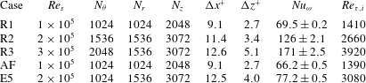
Details of the numerical simulations. The first column is the name with which the simulation will be refereed to in the manuscript. The second column is
 $Re_{s}$
, the shear Reynolds number. The third to fifth columns represent the number of points in the azimuthal, radial and axial directions, while the sixth and seventh columns show the resolution in inner wall units at the mid-gap,
 ${\rm\Delta}x^{+}=[(r_{i}+r_{o}){\rm\Delta}{\it\theta}^{+}]/2$
. The eighth column is the non-dimensional torque
 $Nu_{{\it\omega}}$
. The ninth column is
 $Re_{{\it\tau},i}=u_{{\it\tau},i}d/(2{\it\nu})$
, the frictional Reynolds number at the inner cylinder.
 $Re_{{\it\tau},o}$
can be obtained from
 $Re_{{\it\tau},o}={\it\eta}Re_{{\it\tau},i}$
. The case AF has an imposed axial flow with a mean velocity
 $U_{w}=r_{i}{\it\omega}_{i}/10$
, and the case E5 is the large-gap case with
 ${\it\eta}=0.5$
.

Full details of the numerical simulations are presented in table 1. We mention that the choice of
 ${\it\lambda}_{TR}=2.09$
is arbitrary. Fixing the wavelength of the roll allows for comparison of fluctuations in the bulk across Reynolds numbers, as these depend on roll wavelength (Ostilla-Mónico et al.
Reference Ostilla-Mónico, Verzicco and Lohse2015). We also note that experiments have shown that states with a different number of rolls, and thus different roll wavelengths, are accessible for exactly the same flow parameters (Huisman et al.
Reference Huisman, van der Veen, Sun and Lohse2014; Martinez-Arias et al.
Reference Martinez-Arias, Peixinho, Crumeyrolle and Mutabazi2014). For large Reynolds number, these are generally rectangular vortices, with
 ${\it\lambda}_{TR}>2$
. To demonstrate that our small boxes are sufficient, we refer the reader to Ostilla-Mónico et al. (Reference Ostilla-Mónico, Verzicco and Lohse2015) for a more detailed discussion about the effect of the computational box size, and the effects of
 ${\it\lambda}_{TR}$
on TC flow. There, it is shown that for
 ${\it\eta}=0.909$
computational boxes with
 $n_{sym}=20$
and
 ${\it\Gamma}=2.09$
are large enough for the autocorrelations to smoothly change sign in both axial and azimuthal directions, and in the latter case, to also approach zero. As previously mentioned, the azimuthal (streamwise) correlations decay much faster in TC flow than in PC flow (Tsukahara et al.
Reference Tsukahara, Kawamura and Shingai2006), and thus small boxes can be used.
The axial and azimuthal spectra shown in § 3.4 demonstrate that the mesh is sufficient to capture the small scales. We mention that
 ${\rm\Delta}z^{+}\approx 5$
is a marginally resolved case, while for the azimuthal direction, coarser resolutions of up to
 $r{\rm\Delta}{\it\theta}^{+}\approx 12$
can be used without loss of accuracy or adding numerical dispersion, which changes the physics of the problem.
The simulations were run for an additional
 $50$
large eddy turnover times based on
 $d/U_{i}$
after transient behaviour had died out. In time units based on the frictional velocity
 $u_{{\it\tau}}$
and half the gap width, this is between three and four turnover times. This might seem small when comparing to channels, but it is sufficient for TC flow with pure inner cylinder rotation. The characteristic time for TC flow appears to be
 $d/U_{i}$
. Dong (Reference Dong2008) already showed that the decay of temporal autocorrelations in TC happens in
 $t\approx 3d/U_{i}$
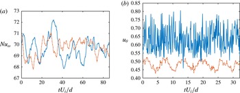
. This fast time scale is further quantified in the left panel of figure 1, which presents the instantaneous non-dimensional torque
 $Nu_{{\it\omega}}=T/T_{pa}$
, where
 $T$
is the torque and
 $T_{pa}$
the torque in the purely azimuthal flow, for the case R1 and the right panel of figure 1, which shows the instantaneous azimuthal velocity at two points for the case R1. The fluctuation time scale at the mid-gap is much slower than that deep inside the boundary layer, probably due to the influence of the large-scale structures.
(a) Instantaneous
 $Nu_{{\it\omega}}$
at inner (solid blue curve) and outer (dash-dot orange curve) cylinders for the R1 simulation. (b) Instantaneous azimuthal velocity near the inner cylinder (
 $r^{+}\approx 12$
, upper blue and solid curve) and in the mid-gap (lower orange and dash-dot curve) for the case R1. The temporal origin is arbitrary. Fluctuations are on time scales of the order
 $O(d/U_{i})$
.

As we will see in more detail in § 3.4, the Reynolds stresses that transport angular velocity are mainly localized in low-wavelength eddies, which have velocities of order
 $O(U_{i})$
. This is not the case in channel flow, where the largest eddies are inactive, i.e. they do not transport Reynolds stresses (Townsend Reference Townsend1976; Hoyas & Jiménez Reference Hoyas and Jiménez2006). Reynolds stresses are transported by boundary layer detachments, or streaks, with velocity scales of
 $O(u_{{\it\tau}})$
, which then naturally lead to the time scales
 $O(d/u_{{\it\tau}})$
for shear transport. However, for the large scales to saturate in energy, much longer times are needed. Large scales are ‘fed’ by detachments from the boundary layers with velocity
 $O(u_{{\it\tau}})$
. This means that the transients in TC flow have time scale
 $O(d/u_{{\it\tau}})$
. Therefore, we define the non-dimensional time based on a large eddy turnover time as
 $\tilde{t}=tU_{i}/d$
.
In the following sections, we will use several kinds of averaging and quantification of fluctuations that are detailed here. The averaging operator of a field
 ${\it\phi}$
with respect to the independent variable
 $x_{i}$
is denoted
 $\langle {\it\phi}\rangle _{x_{i}}$
. We thus define the two different averages:
 $\bar{{\it\phi}}=\langle {\it\phi}\rangle _{{\it\theta},t,z}$
and
 $\hat{{\it\phi}}=\langle {\it\phi}\rangle _{{\it\theta},t}$
. The first type of averaging is analogous to that of homogeneous flows, while the second type is similar to that used in curved channels by Moser & Moin (Reference Moser and Moin1986), where large-scale structures are also present. Using this, we can define two sorts of measures of the fluctuation level. The first is the ordinary definition for homogeneous flows:
 ${\it\phi}^{\prime }=\bar{{\it\phi}^{2}}-(\bar{{\it\phi}})^{2}$
; the second definition is used to separate the effect of the axial inhomogeniety due to the large-scale structure:
 ${\it\phi}^{\star }=\langle \hat{{\it\phi}^{2}}-(\hat{{\it\phi}})^{2}\rangle _{z}$
.
Inner cylinder wall units are defined using
 $u_{{\it\tau},i}$
as a velocity scale and
 ${\it\delta}_{{\it\nu},i}={\it\nu}/u_{{\it\tau},i}$
as a length scale. The mean azimuthal profile is defined as a velocity difference, i.e.
 $U^{+}=(U_{i}-\bar{u}_{{\it\theta}})/u_{{\it\tau},i}$
, where
 $\langle {\it\phi}\rangle _{x_{i}}$
denotes the variable
 ${\it\phi}$
averaged with respect to
 $x_{i}$
.
 $r^{+}$
is the distance to the inner cylinder,
 $r^{+}=(r-r_{i})/{\it\delta}_{nu,i}$
. Outer cylinder wall units are defined using
 ${\it\delta}_{{\it\nu},o}$
and
 $u_{{\it\tau},o}$
, and
 $r^{+}=(r_{o}-r)/{\it\delta}_{{\it\nu},o}$
. The frictional Reynolds number at the outer cylinder is obtained from
 $Re_{{\it\tau},o}\approx {\it\eta}Re_{{\it\tau},i}$
. The non-dimensional distance from the inner cylinder in outer variables is defined as
 $\tilde{r}=(r-r_{i})/d$
, and the angular momentum as
 $L=ru_{{\it\theta}}$
.
3. Results
3.1. Characterization of the large-scale structures
For cases R1–R3, consisting of a radius ratio of
 ${\it\eta}=0.909$
and a stationary outer cylinder, large-scale Taylor rolls exist that fill up the entire domain. Taylor rolls have a fixed axial position and are effectively axisymmetric, even if they are modulated by low-frequency azimuthal waves that do not cause the rolls to vary their spatial location or strength substantially (Ostilla-Mónico et al.
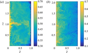
Reference Ostilla-Mónico, Verzicco and Lohse2015). The rolls redistribute angular momentum across the gap, and imprint large-scale patterns that are clearly visible when looking at the velocity field. Figure 2(a) shows a pseudocolour plot of the instantaneous azimuthal velocity for the case R2. A segregation is seen between regions where herringbone-like streaks detach (eject) from the boundary layer and regions where they impact on the boundary layer. We refer to the small-scale structures seen in TC flow as herringbone-like streaks, following Dong (Reference Dong2007). These structures can also be thought of as plumes in the context of convection, as TC flow can be thought of as a system in which angular momentum is transported across the gap.
In figure 2 we can visualize a region of high azimuthal velocity, where these herringbone streaks detach from the inner cylinder boundary layer around
 $\tilde{z}=1$
. Alternatively in the region around
 $\tilde{z}=0$
, streaks detach from the outer cylinder and impact the inner cylinder boundary layer. This detachment/impacting pattern contrasts with the large-gap case E5, shown in the right panel of the figure. Here, the large-scale structures disappear completely, and the herringbone streaks detach and impact all over the cylinder wall. The lack of a large-scale structure was attributed to the asymmetry between the inner and outer cylinders in Ostilla-Monico et al. (Reference Ostilla-Monico, van der Poel, Verzicco, Grossmann and Lohse2014c
). It is worth noting that in some regions of the parameter space, i.e. for weakly counter-rotating cylinders, large-scale structures can reappear again (van der Veen et al.
Reference van der Veen, Huisman, Merbold, Harlander, Egbers, Lohse and Sun2015).
Visualization of the instantaneous azimuthal velocity
 $u_{{\it\theta}}$
for an azimuthal cut for (a) the case R2 and (b) the case E5. The large-scale roll can be clearly seen in (a). These patterns are absent from (b), which shows a larger degree of homogeneity in the axial direction.

We attempted to unfix the rolls by the addition of an axial pressure gradient, which sustains a mean axial flow
 $U_{w}=r_{i}{\it\omega}_{i}/10$
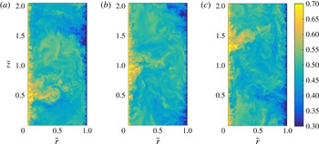
(case AF in table 1). Because this flow is not too strong compared to that induced by the Taylor rolls they do not switch from toroidal rolls to spiral rolls. However, they are no longer fixed in space, and instead they are convected upwards. Thus, the flow again becomes axially homogeneous in a statistical sense. Figure 3 shows a pseudocolour plot of the instantaneous azimuthal velocity for the case AF in three separate instances in time. The large-scale patterns caused by the presence of the underlying roll can be appreciated in all the panels. The (weak) mean axial velocity does not prevent the formation of the Taylor rolls. Instead, as the velocity is ‘small’, the rolls are slowly convected upwards in the computational domain, reappearing on the other side due to the axial periodicity. This is the same as what was seen for the low-Reynolds-number studies of TC flow with an axial pressure gradient, where the Taylor rolls still formed and the axial flow was not large enough to trigger the formation of spirals. The inherent linear instability of the system, present even with an axial flow (Chandrasekhar Reference Chandrasekhar1960a
,Reference Chandrasekhar
b
), causes the formation of these large structures even at high Reynolds numbers.
Visualization of the instantaneous azimuthal velocity
 $u_{{\it\theta}}$
for an azimuthal cut for the case AF at times separated by
 $\tilde{t}=5$
. The large-scale pattern can be clearly seen in (a–c). The roll can be seen to bend slightly upwards due to the presence of an axial mean flow.

Autocorrelation functions for the azimuthal and radial velocities in the axial directions at the mid-gap
 $\tilde{r}=0.5$
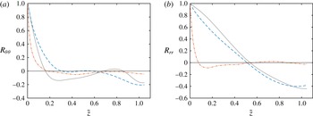
. The signature of the Taylor rolls can be seen on the axial autocorrelations for the cases R1 and AF, but it is absent for the case E5. Symbols: R1, light grey solid curve; E5, orange dash-dot curve; AF, orange dash-dot curve.

To further quantify the disappearance of the large scales, we show in figure 4 the autocorrelations of the azimuthal and radial velocities at the mid-gap in the axial direction for the cases R1, AF and E5. The signature of the rolls, as a large negative autocorrelation at half the roll wavelength, is clearly seen for the cases R1 and AF, both at small gaps with
 ${\it\eta}=0.909$
, and it is absent from the axial autocorrelations of the large-gap case E5. Strangely, an additional minimum for the azimuthal velocity is shown at
 $\tilde{z}=0.25$
, which was seen already in Ostilla-Mónico et al. (Reference Ostilla-Mónico, Verzicco and Lohse2015) consistently at an eighth of the vortex wavelength for different computational domain sizes.
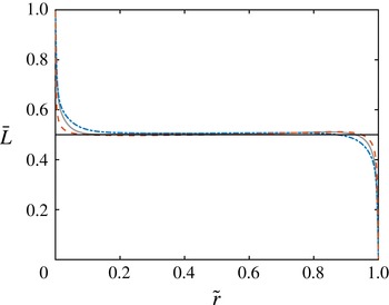
Figure 5 shows the averaged angular momentum
 $\bar{L}$
for the cases E5, AF and R1. Angular momentum is practically constant at the centre of the domain, and equal to the mean angular momentum of both cylinders for all cases. This effect is similar to what is seen at low Reynolds numbers (Marcus Reference Marcus1984; Wereley & Lueptow Reference Wereley and Lueptow1994), and has also recently been observed by Brauckmann et al. (Reference Brauckmann, Salewski and Eckhardt2015) at high Reynolds numbers for several radius ratios and rotation ratios. From this figure, we can clearly distinguish the bulk region, which has constant angular momentum, and the thin boundary layers, where angular momentum has very steep gradients. We note that even if the large-scale structures disappear in the E5 case, angular momentum is still effectively redistributed by turbulence across the entire gap.
Angular momentum
 $\bar{L}$
for the cases R1, AF and E5. A region of constant angular momentum
 $\bar{L}\approx 0.5$
(indicated in the panel by a horizontal line) can be seen in the ‘bulk’. Symbols: R1, light grey solid curve; E5, orange dashed curve; AF, blue dash-dot curve.

3.2. Mean streamwise profiles
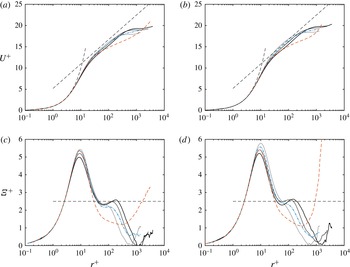
In this subsection we analyse the mean streamwise profiles, focusing first on the small-gap simulations and later on the large-gap case. Figure 6(a,b) shows the mean azimuthal velocity profiles at the inner and outer cylinders in wall units for all cases. In the top two panels, a viscous sublayer and a logarithmic layer can be seen. A classic law of the wall with von Kármán constants of
 ${\it\kappa}=0.4$
and
 $B=5.2$
is shown. For small-gap simulations, the match is quite good for
 $r^{+}<200$
, while in the outer region, large deviations can seen. For the case E5, the local slope in the log layer is very different, highlighting the important effect of the curvature. Indeed, in Ostilla-Monico et al. (Reference Ostilla-Monico, van der Poel, Verzicco, Grossmann and Lohse2014b
) it was shown that for
 ${\it\eta}=0.714$
, the inverse slope in the logarithmic region was quite different from
 ${\it\kappa}=0.4$
.
(a,b) The mean azimuthal (streamwise) velocity profile at the inner (left) and outer (right) cylinders in wall units. Thin dashed lines are
 $U^{+}=r^{+}$
and
 $U^{+}=2.5\log (r^{+})+5.2$
. (c,d) The logarithmic diagnostic function
 ${\it\Xi}^{+}$
at the inner (left) and outer (right) cylinders. The dashed straight line corresponds to
 ${\it\Xi}^{+}=2.5$
on (a–d). Symbols: R1–R3, solid curves from light grey (R1) to black (R3); E5, orange dashed curve; AF, blue dash-dot curve.
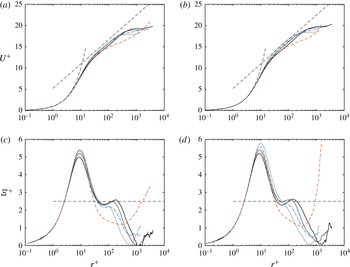
Figure 6(c,d) shows the logarithmic diagnostic function
 $$\begin{eqnarray}{\it\Xi}^{+}=r^{+}\displaystyle \frac{\text{d}U^{+}}{\text{d}r^{+}}.\end{eqnarray}$$
If
 $U^{+}$
is logarithmic, then
 ${\it\Xi}^{+}$
should be horizontal and equal to the inverse of
 ${\it\kappa}$
. This is shown as a dashed line in the plots. For channels, deviations from the universal von Kármán law were proposed by Jiménez & Moser (Reference Jiménez and Moser2007) (based on the overlap arguments of Afzal & Yajnik (Reference Afzal and Yajnik1973)) to have the following shape:
 $$\begin{eqnarray}{\it\Xi}^{+}={\it\kappa}^{-1}+{\it\alpha}y/h+{\it\beta}Re_{{\it\tau}}^{-1/2},\end{eqnarray}$$
where
 $h$
is the channel half-gap, and
 ${\it\alpha}=1$
and
 ${\it\beta}=150$
were obtained from fits to existing data. Bernardini et al. (Reference Bernardini, Pirozzoli and Orlandi2014) found that up to
 $Re_{{\it\tau}}=4000$
(3.2) fits the data well, albeit with slightly modified constants, i.e.
 ${\it\alpha}=1.15$
and
 ${\it\beta}=180$
. However, for PC flow, Pirozzoli et al. (Reference Pirozzoli, Bernardini and Orlandi2014) were not able to quantify the deviations of
 ${\it\Xi}^{+}$
in a systematic way.
In the case of TC flow, fitting an equation analogous to (3.2) for our DNS data in the logarithmic-like region does not lead to a good description of the data. The deviations in the outer region are substantial. However, a tilted S-like behaviour in
 ${\it\Xi}^{+}$
around
 $r^{+}\approx 100$
can be seen for the cases R2 and R3, which is very similar to that one seen in the channel flow and also in PC flow by Pirozzoli et al. (Reference Pirozzoli, Bernardini and Orlandi2014).
When comparing the simulations R1, R2 and R3, we see a strong dependence of the inner layer on
 $Re_{{\it\tau}}$
. The case E5, which we will revisit later, shows a very different structure in the near-wall region due to the large curvature. The peak in
 ${\it\Xi}^{+}$
at
 $r^{+}\approx 10$
does not saturate to a constant value across our simulations. This is probably due to the presence of the underlying large-scale structures. The effect of curvature is also different from what the effective theory by Grossmann, Lohse & Sun (Reference Grossmann, Lohse and Sun2014) predicts, presumably again due to the lack of the underlying larger-scale structures in that theory, and due to the closure assumptions employed. We are unable to draw conclusions about the deviations of
 ${\it\Xi}^{+}$
based only on our DNS data.
For the small-gap simulations, the profiles begin to deviate substantially from the logarithmic law in the bulk, i.e. the region with almost constant angular momentum. The deviations become especially significant from
 $r^{+}>500$
, which corresponds to one tenth of the gap, or only
 $1\,\%$
curvature. The physics of TC flow in this region is dominated by the large-scale rolls. The rolls essentially redistribute angular momentum, and this results in the quasiflat profile for
 ${\it\eta}=0.909$
, and the different slope in the profile for
 ${\it\eta}=0.5$
. The resulting streamwise mean profiles are very different from those seen in PC flow by Bernardini et al. (Reference Bernardini, Pirozzoli and Orlandi2014). We note that TC flow is not Galilean-invariant, and the differences between the two systems could also be due to the effect of a mean rotation. However, in the case of
 ${\it\eta}=0.909$
this mean rotation is very small, and we may attribute the flattening of the profiles to the Taylor rolls. Indeed, the collapse and the smooth transition of the streamwise velocity profiles seen in Brauckmann et al. (Reference Brauckmann, Salewski and Eckhardt2015) happens only for the simulations with a large mean rotation.
We thus may take
 $r^{+}\approx 0.1Re_{{\it\tau}}$
(i.e.
 $\tilde{r}=0.05$
) as an upper bound for the log layer in TC flow for
 ${\it\eta}=0.909$
, because for larger distances from the wall the development of the log layer is constrained by the uniform angular momentum resulting from the presence of the rolls. This means that the effective
 $Re_{{\it\tau}}$
of the simulations decreases substantially, and the possible logarithmic regions extend less into the bulk. If one takes a lower bound for the start of the logarithmic layer to be approximately at
 $r^{+}=3Re_{{\it\tau}}^{1/2}$
(Marusic et al.
Reference Marusic, Monty, Hultmark and Smits2013) and an upper bound at
 $r^{+}\approx 0.1Re_{{\it\tau}}$
due to the dominance of curvature effects and of the rolls, we obtain that the logarithmic layer extends in the
 $r^{+}$
range
 $150<r^{+}<400$
. This is a small range, and does not provide a sufficient separation of scales to accommodate the near-wall cascades that result in a well-developed logarithmic profile. We can take the less conservative lower bound for the start of the log layer of
 $r^{+}\approx 30$
(Pope Reference Pope2000), but even with this bound, the range of length scales is still insufficient.
Therefore, a higher
 $Re_{{\it\tau}}$
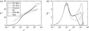
is needed in small-gap TC flow to see a law of the wall comparable to that of channels or pipes. This is shown in more detail in figure 7, which compares the streamwise mean profile and
 ${\it\Xi}^{+}$
in several canonical flows at a frictional Reynolds number of
 $Re_{{\it\tau}}\approx 1000$
. TC flow shows a smaller peak value of
 ${\it\Xi}^{+}$
when compared to the other canonical flows. However, the near-wall region of small-gap TC flow is still surprisingly similar to other canonical flows, given how different all flows are. On the other hand, large-gap TC flow shows significant deviations – something we can expect as the physics is dominated by the curvature and the centrifugal instabilities. Finally, we note that we cannot conclude that we observe a logarithmic layer in our simulations, even if we may speculate based on experimental results (Huisman et al.
Reference Huisman, Scharnowski, Cierpka, Kähler, Lohse and Sun2013) that further DNS at larger
 $Re_{{\it\tau}}$
will lead to the development of a near-wall region with comparable properties to those of other canonical flows.
(a) Mean streamwise component in wall units for several canonical flows. (b)
 ${\it\Xi}^{+}$
for the same flows.

As mentioned previously, the large-gap case shows a very different behaviour (cf. figure 6
a–d). Other approaches to model this behaviour can be taken. Grossmann et al. (Reference Grossmann, Lohse and Sun2014) attempt to calculate the near-wall streamwise profile in TC flow following the spirit of Prandtl’s law of the wall. They use a turbulent diffusivity to account for the extra mixing provided by turbulence. The resulting equations predict a logarithmic layer for the angular velocity with a curvature correction factor
 $A$
equal to
 $A=[1+(r-r_{i})/r_{i}]^{-3}$
for the inner cylinder and
 $A=[1+(r_{o}-r)/r_{o}]^{-3}$
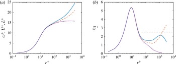
for the outer cylinder. Again we stress that this approach does not consider the effect of the Taylor rolls, which efficiently mix angular momentum in the bulk, so it can only be valid in the near-wall region.
(a) Comparison between angular momentum (purple dash-dot), azimuthal velocity (orange dashed) and angular velocity with curvature corrections (blue solid curve) in wall units for the case E5. (b) Local logarithmic slope for the variables in (a). The horizontal line corresponds to an inverse logarithmic slope of
 ${\it\kappa}=0.4$
.

In figure 8(a), we show the profiles of angular velocity (with curvature corrections), azimuthal velocity and angular momentum in wall units at the inner cylinder for the case E5, in order to compare the consistency of the profiles with a logarithmic layer. To further illustrate this, the right panel shows the local logarithmic slope (or logarithmic diagnostic function) of the three variables. In the near-wall region, the profiles are indistinguishable in the viscous sublayer. Due to the minuscule size of
 ${\it\delta}_{{\it\nu}}$
, the difference between angular momentum and angular velocity is less than 1 % at
 $r^{+}=20$
(
 $\tilde{r}\approx 0.003$
) The profiles only noticeably deviate from each other for
 $r^{+}>50$
. Indeed, in this region, the angular velocity shows the flattest diagnostic function, consistent with the predictions of Grossmann et al. (Reference Grossmann, Lohse and Sun2014), and the numerical simulations of Ostilla-Monico et al. (Reference Ostilla-Monico, van der Poel, Verzicco, Grossmann and Lohse2014b
) at
 ${\it\eta}=0.714$
. However, this log layer does not extend further than
 $r^{+}=300$
, i.e. one twentieth of the gap width. Here, the profiles become consistent with the constant angular momentum in the bulk,
 $\bar{L}=0.5$
, and we see that the diagnostic function for
 $L^{+}$
becomes zero. Therefore, we conclude that even though logarithmic profiles appear for the angular velocity, again these are limited in size to little more than half a decade in
 $r^{+}$
, and do not possess a sufficient range of length scales to sustain the near-wall cascades. We also note that for the case E5, the mean rotation of the system is quite strong, and this may also have an effect on the velocity profile, causing the discrepancies in the bulk region.
3.3. Velocity and pressure fluctuations
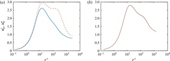
As mentioned in § 2, we have defined two ways to quantify the fluctuations. Figure 9 shows the resulting difference between the two ways for both the case R2 (with fixed rolls and axial inhomogeneity) and the case AF (with no fixed rolls, and thus no axial inhomogeneity). While very significant differences can be seen for the case R2, including the existence (or not) of a second hump, for the AF case the curves collapse on one another and the difference is beneath the temporal convergence error.
To understand this, we must first distinguish the two types of temporal and spatial dependence of the velocity (and pressure) fields seen in small-gap TC flow: the fast small-scale fluctuations inside the rolls, due to the herringbone-like streaks, and the large-scale, quasistationary axial dependence due to the presence of the Taylor rolls. Provided that the rolls are static in the axial direction (cases R1–R3) due to the order of the averaging and subtraction operations only the small-scale fast fluctuations affect
 ${\it\phi}^{\star }$
. The rolls segregate streak detachment regions and streak impacting regions, which have very different velocities, and this spatial dependence is absent using this definition. This is not the case if the rolls are convected (AF simulation) or disappear (E5 simulation). Here, the axial dependence of the flow disappears when computing the mean field, and then both small- and large-scale fluctuations are computed when calculating both
 ${\it\phi}^{\prime }$
and
 ${\it\phi}^{\star }$
, and so they coincide.
Mean fluctuation profiles for azimuthal velocity for case R2 with axial inhomogeneity (a) and case AF with no fixed axial inhomogeneity (b). Symbols:
 $u_{{\it\theta}}^{\prime }$
, dashed orange curve;
 $u_{{\it\theta}}^{\star }$
, solid blue curve.

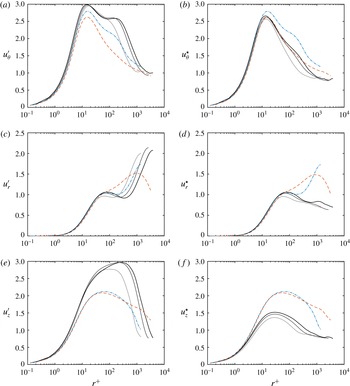
Fluctuation profiles using both types of definition for velocities at the inner cylinder in wall units. Symbols: R1–R3, solid curves from light grey (R1) to black (R3); E5, orange dashed curve; AF, blue dash-dot curve.

Figure 10 shows the velocity fluctuations at the inner cylinder. For the cases R1–R3, the velocity fluctuations are generally either higher (when computed using
 ${\it\phi}^{\prime }$
) or lower (when computed using
 ${\it\phi}^{\star }$
) than those seen for channels at comparable
 $Re_{{\it\tau}}$
(cf. Pirozzoli et al. (Reference Pirozzoli, Bernardini and Orlandi2014) or figure 12). Except for the case AF, there is no presence of a second hump in
 ${\it\phi}^{\star }$
, and the level of fluctuations slightly increases with
 $Re_{{\it\tau}}$
, as expected. The difference between the two ways of quantifying the fluctuations is apparent here. The axial inhomogeneity causes a significant increase in the measurement, especially in the bulk region, where the structure is more pronounced.
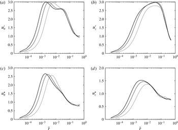
Velocity fluctuations are also shown with the horizontal axis in outer units in figure 11. A reasonable collapse can be seen in an ‘overlap’ layer. This layer is defined between
 $r^{+}>100$
and
 $\tilde{r}<0.2$
, i.e.
 $r^{+}<0.4Re_{{\it\tau}}$
. Here,
 $u_{{\it\theta}}^{\prime }$
and
 $u_{z}^{\prime }$
show a local profile that is consistent with logarithmic behaviour. This can mean that a region in which overlap arguments are valid exists in TC flow. However, DNS with larger
 $Re_{{\it\tau}}$
are needed to sufficiently decouple the scales and obtain convincing evidence for this overlap layer, with logarithmic profiles in both the mean velocities and the pressure and velocity fluctuations.
Fluctuations of the azimuthal (a,c) and axial (b,d) velocity components for the cases R1, R2 and R3 in outer units. Regardless of the way of calculating the fluctuations, an overlap region where the fluctuations collapse can be seen in (a–d). Symbols: R1–R3, solid curves from light grey (R1) to black (R3).

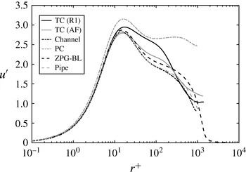
This is further quantified in figure 12, which compares the azimuthal (streamwise) velocity fluctuations at the inner cylinder for the cases R1 and AF with those of the streamwise velocity for several canonical flows at around
 $Re_{{\it\tau}}\approx 1000$
. Except for PC flow and the case R1, a remarkable agreement in the value of
 $u^{\prime }$
at the peak of
 $r^{+}\approx 12$
is obtained, including the data from the case AF. The case R1 has more fluctuations than the other cases. This might be expected, both for the reasons mentioned previously about the axial inhomogeneity (notable when comparing the cases AF and R1) and because in TC flow we are driving a secondary flow due to a centrifugal instability, and this can also affect the level of fluctuations (the level is lower when comparing only the fluctuations coming from the streaks). This second effect is probably the cause of the smaller level of fluctuations seen in the case E5 even when the large-scale structure is absent. The addition of an axial flow or of a large curvature increases the level of fluctuations, especially those of the radial and axial velocities. This is the reason we see both a second peak in
 $u_{{\it\theta}}^{\prime }$
for high
 $r^{+}$
in the case AF and higher values of
 $u_{r}^{\prime }$
and
 $u_{z}^{\prime }$
, especially near the mid-gap for both the cases E5 and AF.
Streamwise velocity (azimuthal velocity for TC flow) fluctuations in wall units for the cases R1 and AF at the inner cylinder, and some canonical flows.

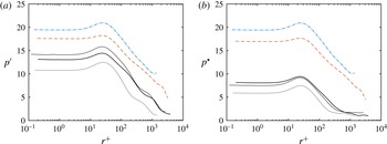
Clear logarithmic behaviour is also seen for
 $p^{\prime }$
in figure 13, as well as a reasonable collapse of the data in this region for the cases R2 and R3 when looking at the
 $p^{\star }$
quantification. This behaviour is consistent with the existence of an overlap region. In addition, the pressure fluctuations in the case AF are almost three times as large as for the case R1, but this is due to the way the axial pressure gradient is imposed – with a time-varying magnitude.
Fluctuation profiles using both types of definition for velocities and pressure at the inner cylinder in wall units. Symbols: R1–R3, solid curves from light grey (R1) to black (R3); E5, orange dashed curve; AF, blue dash-dot curve.

3.4. Velocity spectra
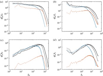
Taylor rolls contain a significant amount of the kinetic energy in the flow, both in the bulk and in the boundary layer. This is quantified in figure 14, which shows the azimuthal and axial spectra of the azimuthal and radial velocity for
 $r^{+}\approx 12$
(near the wall) in outer units. The Taylor rolls are associated with the lowest wavelengths in the axial spectra, and these show a prominent maximum at the fundamental wavelength. This signature is present not only for
 ${\it\phi}_{{\it\theta}{\it\theta}}$
but also for the radial velocity spectra
 ${\it\phi}_{rr}$
for the small-gap cases. For the case E5, this signature is not present, consistent with the fact that the rolls have faded.
Furthermore, all small-gap cases show a maximum in the co-spectra
 ${\it\phi}_{{\it\theta}r}$
(not plotted here) corresponding to the wavelength of axisymmetric Taylor rolls, i.e.
 $k_{{\it\theta}}=0$
,
 $k_{z}=2{\rm\pi}/{\it\lambda}_{TR}$
. If present, the rolls dominate the convective transport of angular velocity through the Reynolds stresses in the boundary layer. This means that Taylor rolls are not inactive in the sense of Townsend (Reference Townsend1976) and Hoyas & Jiménez (Reference Hoyas and Jiménez2006). Rolls actively transport (or redistribute) the angular velocity current. This result, well known at low Reynolds numbers, is extended here to the high Reynolds numbers analysed. Furthermore, unlike the large-scale structures in channel flow and PC flow, the rolls may be considered to be ‘attached’ to the wall, and their presence is felt inside the boundary layer. No signature of this large-scale roll can be seen for the case E5, and the transport of the conserved quantity in the boundary layer happens through fluctuations.
Premultiplied azimuthal (a,c) and axial (b,d) spectra for azimuthal and radial velocity components for all simulations at
 $r^{+}\approx 12$
. Symbols: R1–R3, solid curves from light grey (R1) to black (R3); E5, black dashed curve; AF, black dash-dot curve.

It might seem strange that such a large wavelength appears with the radial (wall-normal) velocity near the wall, considering the impermeability condition. In channels and PC flow, the large-scale structures reflect only the streamwise velocity near the wall. In TC flow, however, if present, they reflect both the streamwise and the wall-normal velocity near the wall. This is probably due to the inherent linear instability of TC flow, which causes the formation of the rolls.
Figure 15 shows that rolls also dominate the spectra at the mid-gap for the small-gap cases. Once again, a prominent sawtooth behaviour in the axial spectra can be seen for the lowest wavenumbers. The spectra are consistent with the experiments by Lewis & Swinney (Reference Lewis and Swinney1999), and show neither
 $-1$
nor
 $-5/3$
scaling. This is unlike the case of pipe flow (Perry et al.
Reference Perry, Henbest and Chong1986), for which a
 $-1$
scaling was found, and also unlike the case of curved channel flow (Hunt & Joubert Reference Hunt and Joubert1979), which shows the expected
 $-1$
scaling laws for the streamwise energy spectra in the streamwise direction. Also, the axial velocity spectra in the azimuthal direction do not show a
 $-5/3$
exponent, consistent with the experiments of Perry et al. (Reference Perry, Henbest and Chong1986).
Premultiplied azimuthal and axial spectra for the azimuthal components for all simulations at mid-gap. Symbols: R1–R3, solid curves from light grey (R1) to black (R3); E5, orange dashed curve; AF, blue dash-dot curve.

When compared to other flows, it seems clear that for small-gap TC flow, the large-scale structures are responsible for the transport of the conserved quantity. The fluctuations transport very little on average, even though their instantaneous transport can be orders of magnitude higher than the mean transport (Huisman et al. Reference Huisman, van Gils, Grossmann, Sun and Lohse2012). For large-gap TC flow, transport happens through the small-scale fluctuations, as the rolls do not form. We note that unlike in channel flow and curved channel flow, the Reynolds stresses in TC flow are maximal at the mid-gap to satisfy the conservation of angular velocity current (torque). In PC flow, large-scale structures also form, but these are also inactive, i.e. they do not transport shear (Avsarkisov et al. Reference Avsarkisov, Hoyas, Oberlack and García-Galache2014). Therefore, it seems that small-gap TC flow is the only flow examined to date that involves transport by Reynolds stresses of a conserved quantity, in this case angular velocity, by large-scale structures that are attached to the wall. We note that Lozano-Durán, Flores & Jiménez (Reference Lozano-Durán, Flores and Jiménez2012) do see large-scale wall-attached active structures in channel flow when using an analysis based on a full quantification of three-dimensional structures (Qs) instead of the more ‘classic’ co-spectra. They find very few countergradient (i.e. negative transport) wall-attached eddies, while the Taylor roll in TC flow has both a gradient and a countergradient part (Huisman et al. Reference Huisman, van Gils, Grossmann, Sun and Lohse2012; Ostilla-Monico et al. Reference Ostilla-Monico, Huisman, Jannink, van Gils, Verzicco, Grossmann, Sun and Lohse2014a ). To further understand the differences, an analysis of TC flow using the same method is necessary, and will lead to a better one-to-one comparison. We may also speculate that a similar behaviour could also be present in Rayleigh–Bénard (RB) flow, the flow in a fluid layer heated from below and cooled from above. RB flow also shows a linear instability (Chandrasekhar Reference Chandrasekhar1981) and persistent large-scale structures that cover the entire gap (Ahlers, Grossmann & Lohse Reference Ahlers, Grossmann and Lohse2009).
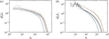
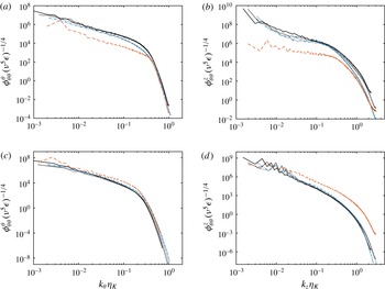
Finally, in figure 16 we show the azimuthal velocity spectra in Kolmogorov units, using the Kolmogorov length scale
 ${\it\eta}_{K}={\it\nu}^{3/4}{\it\epsilon}^{-1/4}$
, for normalization, where
 ${\it\epsilon}$
is the energy dissipation rate, both at
 $r^{+}\approx 12$
and at the mid-gap. At low wavenumbers the energy is dominated by the rolls, but at high wavenumbers some collapse between the small-gap cases can be seen both for azimuthal spectra and for the axial spectra at the mid-gap. All azimuthal spectra show a similar shape, both inside the boundary layer and at the mid-gap. The characteristic bend corresponding to
 $10{\it\eta}_{K}$
can be appreciated in both left panels. Meanwhile the axial spectra can show different shapes. The most notable lack of collapse is seen for
 $r^{+}\approx 12$
in the axial spectra, but this is probably due to the different size of the herringbone streaks, which scale with
 $Nu_{{\it\omega}}$
and not
 ${\it\eta}_{K}\sim Nu_{{\it\omega}}^{-1/4}Re_{s}^{-1/2}$
, or due to dispersive errors caused by insufficient resolution, especially seen in the tails of the spectra of the largest runs. On the other hand, a remarkable collapse for all cases for the azimuthal spectra, and for all small-gap cases for the axial spectra, is seen for both spectra at mid-gap. Similar spectra and collapses are seen for the other two velocity components, not shown here.
Azimuthal (a,c) and axial (b,d) spectra for the azimuthal velocity for all simulations at
 $r^{+}\approx 12$
(a,b) and mid-gap (c,d). Symbols: R1–R3, solid curves from light grey (R1) to black (R3); E5, orange dashed curve; AF, blue dash-dot curve.

4. Summary and outlook
Four large DNS simulations of small-gap, and one of large-gap Taylor–Couette flow were conducted, reaching frictional Reynolds numbers of
 $Re_{{\it\tau}}=4000$
. In the small-gap case, large-scale structures, known as Taylor rolls, form in the bulk and play an active role in the system dynamics by transporting angular velocity through Reynolds stresses. The rolls are ‘attached’ to the cylinders, and even deep inside in the boundary layers, for
 $r^{+}\approx 12$
, their signature is significant in the
 ${\it\phi}_{{\it\theta}r}$
co-spectra. Adding a weak axial pressure gradient was found to advect the rolls slowly, but not to weaken them significantly, in agreement with what is seen at low Reynolds numbers. This axial pressure gradient was weak enough only to convect the rolls. Different results and flow topologies could arise from stronger gradients. The rolls’ signatures were still present in axial spectra in the boundary layer, and in the axial correlations of radial velocity. These structures were notable in the large-gap case, where the transport of the conserved quantity is by small-scale fluctuations.
The mean velocity profile of TC flow has considerable differences to the Prandtl–von Kármán log-layer profile
 $U^{+}={\it\kappa}^{-1}\ln y^{+}+B$
with
 ${\it\kappa}\approx 0.4$
and
 $B\approx 5.2$
. In the small-gap case close to the walls,
 ${\it\kappa}$
is very close to
 $0.4$
, while
 $B$
is slightly lower and dependent on Reynolds number. With increasing distance from the wall, large deviations from the logarithmic law are found. The Taylor rolls redistribute angular momentum, which results in an essentially flat angular momentum profile, even for curvatures of
 $1\,\%$
. This is consistent with the notion that curvature effects are orders of magnitude larger than expected by mere dimensional analysis (Bradshaw Reference Bradshaw1973). For the large-gap case, a degree of logarithmic behaviour can be seen for the angular velocity, consistent with the prediction of Grossmann et al. (Reference Grossmann, Lohse and Sun2014), and similar to what was already seen for
 ${\it\eta}=0.714$
in Ostilla-Monico et al. (Reference Ostilla-Monico, van der Poel, Verzicco, Grossmann and Lohse2014b
). This logarithmic region has a very different inverse slope
 ${\it\kappa}$
, and only extends less than half a decade in
 $r^{+}$
for
 $Re_{{\it\tau}}\approx 3100$
, due to the mixing of angular momentum in the bulk. The nature of this region seems to be very different from the classical law of the wall.
Fluctuation profiles were also analysed. When adding a mean axial flow, the azimuthal velocity fluctuations presented coincide with those seen in other canonical flows at comparable
 $Re_{{\it\tau}}$
. The velocity fluctuations were found to collapse when plotted in outer units, indicating the presence of an overlap region. Based on these findings, we expect that simulations at higher
 $Re_{{\it\tau}}$
will provide enough decoupling of scales for a large overlap region to form. This will allow logarithmic profiles to develop in both the mean azimuthal velocity and the velocity and pressure fluctuations. Once again, the large-gap case was found to have a different behaviour. No rolls were present and the level of fluctuations was smaller at a comparable
 $Re_{{\it\tau}}$
.
Further investigations should also look at the effect of strongly counter-rotating cylinders, which have a significant Rayleigh-stable region, or even pure outer cylinder rotation, which is completely Rayleigh-stable, and how this affects the large-scale structures. Finally, additional simulations with a larger choice of pressure gradients, both in the axial direction, as done in this manuscript, and in the azimuthal direction, to provide a mixed Couette–Poiseulle flow, will be useful to increase our understanding of the system.
Acknowledgements
We would like to thank M. Bernardini, S. Pirozzolli, E. P. van der Poel and P. Orlandi for various stimulating discussions. We acknowledge that the results of this research have been achieved using the PRACE project 2013091966 resource CURIE based in France at Genci/CEA. We also acknowledge support by an ERC advanced grant.