

1 Introduction
Many workers fear a decline in the pensions they expect to receive from Social Security or their employer. In several countries, this concern is motivated in part by the combination of pay-as-you-go financing with an ageing population. This apprehension is also justified by the large number of employers who have shut down or frozen their defined benefit pension plans in the last two decades. Additionally, recent empirical evidence shows that workers make suboptimal savings and investment decisions in their defined contribution plans (e.g. see Choi, Laibson, Madrian, and Metrick, Reference Choi, Laibson, Madrian, Metrick, McCaffrey and Slemrod2006).
Assuming that people would work a few more years can improve the outlook in this context. For example, Munnell, Buessing, Soto, and Sass (Reference Munnell, Buessing, Soto and Sass2006) estimate that the expected decline in Social Security replacement rates could be offset by working for an additional three and a half years. Using the Health and Retirement Study (HRS), Au, Mitchell, and Phillips (Reference Au, Mitchell and Phillips2005) evaluate that many workers do not have sufficient savings to maintain their pre-retirement level of consumption, but delaying retirement by three years would make up for about half of the savings shortfall. Butrica, Smith, and Steuerle (Reference Butrica, Smith and Steuerle2006) show that if work and the Normal Retirement Age (NRA) were extended by five years in the US, retirement income would be preserved and Social Security deficits eliminated.
Based on these examples, it is tempting to perceive working longer as a silver bullet to current pension problems. Unfortunately, traditional pension analysis tools provide only limited insight when it comes to evaluating the potential merit of that strategy. For instance, previous studies had to rely on an arbitrarily specified increase in the retirement age for their illustrations. Furthermore, the measures that were analyzed – retirement income, savings, and degree of funding – inevitably improve when longer work is presumed. Since these measures do not reflect the disutility cost associated with the additional years of work, they create a positively biased picture.
To address these limitations, we assume a different standpoint and approach the problem from a utility-based perspective. In particular, we build our analysis on a life-cycle framework which takes into account the utility of leisure. The fundamental question that we are asking is not whether working longer can increase retirement income, but can it improve materially the worker's overall welfare. The other novelty in our treatment is that we let the retirement age be endogenously determined by the model, unless an external constraint or shock applies first. This twofold view of retirement is in line with Munnell's (Reference Munnell2006) report that, of those HRS respondents retiring by age 65, 65.2% did so voluntarily, 18.0% claimed health reasons, 7.3% were laid off, 5.7% attributed it to a closed business and 3.7% to family reasons.
Our model is most closely related to a recent stream of literature by Dybvig and Liu (Reference Dybvig and Liu2005), Farhi and Panageas (Reference Farhi and Panageas2005), and Lachance (Reference Lachance2003) where a one-time endogenous retirement decision is added to a standard life-cycle model. In order to obtain tractable solutions to the problem, these papers considered the special case of an infinite horizon and stationary parameters. In this paper, we extend these models so that they can accommodate more realistic retirement-related assumptions. In particular, one of the main innovations in the model is the addition of an exogenous retirement constraint, which can be stochastic or deterministic. Other realistic features added to the model include a finite lifetime, time-dependency in income, and mortality, pensions, and early/delayed retirement provisions. To our knowledge, this is the first paper that derives the solution to a life-cycle model where a stochastic retirement date can be determined either endogenously or exogenously.
Contrarily to previous reports that working longer can improve retirement income significantly, we find that this strategy has relatively little impact on welfare. This result is expected for those who are forced to retire by external factors. The point is more subtle for the predominant scenario with voluntary retirement. If we had a model with a fixed retirement horizon, assuming longer work could result in either a welfare gain or a welfare loss. When retirement is endogenous, we have a different story. In that case, the marginal benefit of an additional period of work should be reasonably close to its marginal cost; otherwise, retiring at the endogenous date would not be optimal. Therefore, whatever can be gained in income is almost completely offset by a corresponding loss in leisure utility.
The applicability of these results can best be seen in the context of public pension reforms. Given the major improvements in longevity over the last decades, pay-as-you-go public pension systems face important financing difficulties.Footnote 1 To restore fiscal sustainability, these public systems must either increase taxes, reduce benefits, or use a combination of these strategies. Observers such as Gramlich (Reference Gramlich2006) have suggested that a further increase in the NRA should be part of the next round of Social Security reforms. The proposed strategy would reduce the number and level of benefit payouts, which should induce people to work longer and augment payroll and income tax revenues. This type of proposal is likely to be evaluated with traditional measures such as retirement income and funding level (e.g. see Butrica, Smith, and Steuerle, Reference Butrica, Smith and Steuerle2006). We use our model to highlight some important framing and bias issues inherent to these measures.
Another application of our model is to show how adopting a ‘combination approach’ can enhance the effectiveness of a policy that increases the NRA, both in terms of improving public finances and individual welfare. With that tack, a raise in the NRA is paired with a set of non-financial measures, which can be broadly categorized as (1) removing constraints to longer work, (2) reducing the disutility cost of work at older ages, and (3) addressing cognitive limitations and information barriers that can result in suboptimal early retirement. As these measures improve the individual's welfare, they can help offset part of the loss created by the reduction in benefits. At the same time, more people would be able and willing to work longer, which would benefit public finances through an increase in tax revenues. The recent UK pension reform offers a concrete example of our combination approach. Besides recommending an increase in the State Pension Age from 65 to 68, that reform put forward a wide range of proposals which should induce and enable longer worklives. These measures are in line with the suggestions we outlined above and it would be interesting to consider this type of policy in the US if their implementation in the UK proves to be successful.
The remainder of this paper is structured as follows. The model is presented and solved in Section 2. We use it to examine our question in Section 3. Section 4 describes the combination approach in more detail and its application to the UK case. Section 5 concludes and suggests some directions for future research.
2 Model
Despite the existence of an extensive literature on life-cycle modeling, little attention has been given to the welfare aspect of pension reductions and longer work. So far, this problem has been mostly analyzed from a cash flows perspective in a static setup. To examine this issue in a more suitable dynamic framework, traditional life-cycle models of optimal investment and consumption (e.g. Merton, Reference Merton1971; Bodie, Merton, and Samuelson, Reference Bodie, Merton and Samuelson1992) need to be adapted because they typically have a fixed retirement horizon. For that purpose, it is useful to consider a recent stream of literature where a one-time endogenous retirement decision is introduced in a classical life-cycle model (e.g. Dybvig and Liu, Reference Dybvig and Liu2005; Farhi and Panageas, Reference Farhi and Panageas2005; Lachance, Reference Lachance2003).Footnote 2 We build on this literature and develop a flexible formulation which provides analytical insight and accommodates a wider range of realistic retirement income structures (e.g. finite lifetime, time-dependency in income and mortality, outside pensions, and early/delayed retirement provisions). The technique used to derive the model's solution is an extension of the dual approach suggested in Karatzas and Wang (Reference Karatzas and Wang2000).
2.1 Lifespan and retirement
The problem to be solved begins at time 0 and the individual can live for a maximum of T years. The probability that the individual survives from time 0 to time t is denoted by p t. This function can represent any realistic mortality table. To incorporate mortality in the model, we use the standard approach and discount utility by a factor p t.
We assume that the individual works full-time until he retires completely and permanently. Our model allows the retirement date to be either endogenous (voluntary) or exogenous (involuntary). To make a distinction between these two types of retirement dates, we introduce some new notation τendo and τexo. According to expected utility theory, individuals should retire at time τendo when retiring yields more utility than continuing to work. However, it might not be realistic to assume that individuals have a perfect ability to delay retirement at will, especially at older ages. Indeed, an important proportion of the HRS respondents reported retiring involuntarily. While disability and poor health are a major cause of suboptimal early retirement, various other issues such as lay-offs and mandatory retirement can play a role. To take these various factors into account, we introduce the concept of an age τexo at which the individual would be forced to retire for any reason. With the notation τendo and τexo, we can then model our retirement age as a stopping time τ=min[τendo,τexo]. In other words, we assume that the individual will retire when this decision maximizes his utility, unless external factors force him to retire earlier.
The τexo notation will be used extensively throughout this paper. Since this modeling element was not used in the previous literature, some clarifications are in order. In this paper, we want to keep the concept of a forced retirement as general as possible. We think of τexo as any factor that would cause the individual to retire early, although from a utility perspective, continuing to work would have been optimal. From a technical point of view, we want τexo to be flexible enough to accommodate both fixed constraints (e.g. a mandatory retirement age) and retirement shocks (e.g. disability). Accordingly, we assume that the probability of being forced to retire at time t can be represented by any probability distribution, including truncated distributions. To describe changes in the distribution of τexo, it will be convenient to characterize it by its expected value E[τexo]. Therefore, in our analysis, an improvement in the ability to work longer translates into an increase in E[τexo].
Later, it will be interesting to consider increases in E[τexo] for two reasons. First, it can be relevant to take into account the effect of natural trends which make it easier to remain in the labor force longer. Second, it can be interesting to think in terms of policies that can increase welfare by improving the ability to work longer. A wide variety of factors could lead to increases in E[τexo], we mention a few here. Improvements in health would reduce the probability of being forced to retire for disability reasons. Technological innovations could facilitate work at older ages. Some policies could also help by promoting work at older ages, preventing age discrimination, and removing mandatory retirement ages when they exist. We will come back to this policy aspect in Section 4 and discuss it further.
2.2 Preferences
Time preferences are represented by a discount factor β>0 and the individual's discounted utility is given by a function
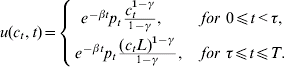
According to (1), the individual's utility of consumption is modeled with a power utility function with a coefficient of relative risk aversion γ. When he ceases to work, the individual also derives increased utility from leisure. To take this utility of leisure into account, we follow the approach in related works by, among others, Dybvig and Liu (Reference Dybvig and Liu2005) and Fahri and Panageas (Reference Farhi and Panageas2005) and multiply consumption by a parameter 1⩽L<∞ after retirement.Footnote 3 With that approach, the utility of leisure before retirement is normalized to L=1. The greater the value of the parameter L after retirement, the more the individual values leisure (or dislikes work). While we use a fixed parameter L for simplicity, it would be possible to vary L with age.
2.3 Labor income and pensions
In the working years, the individual earns labor income at a deterministic rate  t. This income can be subject to both income and Social Security taxes. We denote by y t the after-tax labor income rate. After retiring, the individual may be eligible to receive a pension (i.e. an annuity). We use a general function a τ,t to denote the pension payments that the retiree would receive at time τ⩽t⩽T, given retirement at time τ. This function can represent a wide variety of pension designs. For instance, it can be used to model a Social Security pension, an employer-provided pension, or a combination of both.Footnote 4 Given that we assume the labor income process is known, the level of the annuity payments can be any function of past salaries. The annuity payments can also be indexed and adjusted to reflect early/delayed retirement provisions.
2.4 Investments and wealth process
The individual can allocate his wealth between two assets, one risky and one risk-free. His investment in the risky asset is represented by a process πt. This process is not constrained and there are no limits on borrowing and short selling. The risk-free asset earns a return r f and the risky asset's return is given by the differential equation

where 0<r f<μ, 0<σ<∞, and {ωt, 0⩽t⩽T} is a Brownian motion process.
The individual is endowed with initial capital W 0=w and his wealth process is defined by the equation

We do not impose a non-negative condition on the wealth process, but we prevent the worker from borrowing more than he can repay.
2.5 Optimization problem
We assume that the individual makes consumption, portfolio, and retirement decisions such that his expected discounted utility is maximized. We use a function R(w τ,τ) to represent the portion of this utility which is derived after retirement. This function R(w τ,τ) is the solution to a fairly typical optimization problem, which is given in Appendix A. It follows that we can define the individual's expected discounted utility before retirement with the expression
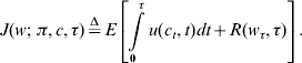
The individual's optimization problem before retirement is to find the triple (π,c,τ) with τ⩽τexo that maximizes (4) and satisfies the wealth process in (3). The value function of this problem is denoted by

Solving for the optimal retirement strategy τ poses a difficulty since τ does not represent a fixed retirement horizon. In other words, we cannot obtain τ simply by solving a first-order condition. This hurdle can be overcome by using an approach suggested by Karatzas and Wang (Reference Karatzas and Wang2000) for a problem of optimal consumption and investment with a discretionary stopping time. To solve our problem, we must adapt Karatzas and Wang's (Reference Karatzas and Wang2000) approach to incorporate elements such as labor income, pensions, and exogenous retirement shocks.
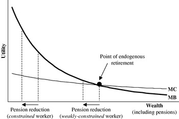
We present our solution for the value function V(w) and the optimal decisions (π,c,τ) in Appendix A. This solution has a familiar structure, with the exception of the retirement horizon which now results from a combination of endogenous and exogenous factors. To understand intuitively how these factors affect the problem, one can think in terms of the marginal benefit (MB) and marginal cost (MC) associated with delaying retirement by one period. The reader can find the formulas for MB and MC at the end of Appendix A. MB is equal to the increase in income times the marginal utility of wealth. MC can be described as decreasing with wealth and increasing with the utility of leisure. The difference MB−MC also decreases with wealth. To explain our results intuitively, it will be convenient to work with the graphical representation of MB and MC as a function of wealth, which is given in Figure 1. In that figure, MB decreases quickly and then flattens out because it is proportional to the marginal utility of wealth.
Delaying retirement by one period: marginal benefit (MB) vs. marginal cost (MC)

Since workers make utility-maximizing decisions, it is optimal to delay retirement when the associated benefit is greater than the cost, i.e. when MB>MC. In that case, working longer increases welfare by MB−MC>0. When wealth is relatively low, MB is much higher than MC and it is optimal to work longer. As wealth increases, the additional income becomes relatively less valuable and the welfare gain MB−MC decreases. Eventually, the welfare gain will converge to zero and it will be optimal to retire when MB=MC. However, not all workers will be able to reach that point. For some, an exogenous retirement shock will force them to retire when MB>MC and work is still otherwise desirable.
Figure 1 shows that workers with a greater wealth (including pensions) are closer to retirement. For example, good investment performance should lead to early retirement. This prediction seems to be supported by recent empirical evidence.Footnote 5Figure 1 also illustrates that workers will be nearer retirement if they have a relatively low MB or high MC. Using the formulas for MB and MC that we give in Appendix A, we predict that early retirement is more likely when: (1) pensions replace a larger fraction of labor income, (2) there is a small increase in pensions for delayed retirement, and (3) the utility of leisure is relatively high. Furthermore, our analysis in Appendix A suggests that those with a greater life expectancy should retire later.Footnote 6
3 Pension reductions, working longer, and welfare losses
We now turn to the question of interest in this paper, which is whether working longer can effectively decrease the impact of a pension reduction on welfare. Here, the expression ‘pension reduction’ encompasses a variety of situations that adversely affect one's retirement income. For instance, this could be through a change in a defined benefit formula, an increase in the normal retirement age, a change in the early retirement provisions, a reduction in the contributions made by an employer to a 401(k) plan, or lower-than-expected returns on retirement savings.
The issue investigated here is not whether working longer improves welfare after a pension reduction; this is obviously the case when retirement is endogenous. The more interesting question is whether this improvement is significant enough to make working longer an effective solution to pension problems. Note that this question cannot be answered with an analytical proof given that the ‘magnitude’ of welfare gains is a relative concept. Nevertheless, we show here how we can use our model to build a strong case to support the notion that working longer does little to improve welfare. First, in Section 3.1 we use Figure 1 to explain intuitively the potential magnitude of welfare gains associated with working longer. Second, in Section 3.2. we use a numerical analysis and some sensitivity tests to support our theoretical predictions. To simplify the analysis, we restrict our attention to two extreme types of workers. The weakly constrained worker is one who is typically able to retire endogenously at time τendo, but may be forced to retire at time τexo in a few scenarios. By contrast, the constrained worker is one who is forced to retire at time τexo most of the time. These cases can be viewed as bounds for the range of likely results.
3.1 Intuition
In the context of Figure 1, a pension reduction can be interpreted as a reduction in wealth, i.e. as a shift to the left on the horizontal axis. This shift implies that it will be optimal for both types of workers to delay retirement as this would increase their welfare by MB−MC. However, this strategy will not be an option for the constrained worker as he is already working as long as possible, i.e. until time τexo. While the weakly constrained worker will be able to delay retirement, the magnitude of his resulting welfare gain MB−MC converges to zero around the endogenous retirement date. Therefore, for both types of workers, we do not expect that working longer will improve their welfare considerably.
If we assume an alternative and interesting standpoint, a natural question arises: When can working longer increase welfare significantly? As Figure 1 shows, larger welfare gains associated with working longer can be found by considering workers who retire much before their optimal retirement date. In our model, this happens when workers are forced to retire early at time τexo. This suggests that potentially interesting welfare gains could arise if the ability to work longer was improved. To evaluate the potential of that strategy, we consider various increases in E[τexo] in our numerical analysis in Section 3.2.
3.2 Numerical example
In this section we show that the predictions we made in Section 3.1. are not an artifact of the way we have drawn and interpreted Figure 1. To support these predictions, we performed a variety of numerical tests. Due to space constraints, we present only one of these sensitivity tests here. The results of the other tests were similar and are available in a supplement to this paper upon demand. When choosing the assumptions for these illustrations, we take advantage of some of our model's features, which allows us to produce credible illustrations in a realistic pension context. For instance, the models with endogenous retirement cited earlier would have prevented us from using time-varying mortality rates or incorporating pension payments after retirement.
Rather than using a hypothetical case for the pension reduction, it will be interesting to consider the real-life case of the scheduled increase in the Normal Retirement Age (NRA) of the US Social Security system. Though the NRA was 65 years old for a long period of time, this age will be raised to 67 years old over the next two decades. Currently, the NRA is about 65.5 years old and its future increase from age 65.5 to age 67 can be interpreted as a form of pension reduction.
We use the following base case scenario for our numerical illustrations. The worker is assumed to be 55 years old, with initial income y 0=$25,000 and savings w=$100,000. The worker is subject to an exogenous retirement shock which is expected to occur at age 65.5. For the utility of leisure, we consider two cases. The weakly constrained worker values leisure highly (L=2.50) and he initially expects to retire early at age 61.7. The constrained worker values leisure much less (L=1.25) and initially expects to retire at age 65.4, which is very close to the assumed value of E[τexo].Footnote 7 After retiring, the individual derives income from two sources: personal savings and a Social Security pension. This pension is modeled according to the current US Social Security system's rules. These rules and the other assumptions used to produce our illustrations are detailed further in Appendix C.
Since welfare gains are expressed in terms of utility, their magnitude can be difficult to interpret. Therefore, we take an approach commonly used in the literature and convert the welfare gains into a ‘wealth-equivalent’ measure in dollars. More precisely, recall that the individual's lifetime utility is measured by the value function V(w) given in equations (5) and (14). Let V(w) and V*(w) denote the worker's utility respectively before and after an increase in work. The wealth-equivalent cost of this additional work can be obtained by solving for x in V(w+x)=V*(w).
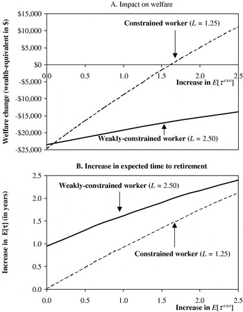
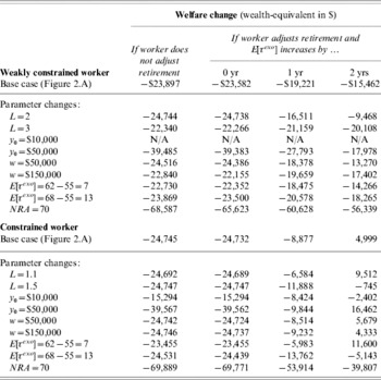
We can use this approach to evaluate the welfare losses associated with the 1.5-year increase in the NRA. To capture the effect that delaying retirement has on welfare, we first compute the welfare losses for the case where the worker is not able to adjust the retirement date in response to the NRA increase. The welfare loss in this case would be −$23,897 for the weakly constrained worker and −$24,745 for the constrained worker (see Table 1). These losses represent 10% of the initial value of the retirement benefits. We then show in Figure 2.A how these welfare losses are affected when the worker is able to delay retirement. The associated increase in the expected time to retirement is given in Figure 2.B.
Impact of a 1.5-year increase in social security's NRA
Note: L is a parameter which increases with the utility of leisure. E[τ] denotes the expected time to retirement and an increase in E[τexo] represents an improvement in the ability to remain in the workforce. The parameters and assumptions used to generate these results are detailed in Appendix C.

Sensitivity analysis of Figure 2.A's results

Note: Results computed with the base case parameters and assumptions described in Appendix C except for the listed parameter change. In terms of notation, L is leisure, y 0 is the initial labor income, w is the initial wealth, E[τexo] is the expected time until exogenous retirement, and NRA is Social Security's normal retirement age. In the case where y 0=$10,000, our model does not apply; it is optimal to retire immediately at age 55.
We start by analyzing the results for our basic scenario, i.e. for the case with E[τexo]=0 in Figure 2. In that case, delaying retirement can do little to improve welfare losses. For the constrained worker, this is not surprising since he is already expected to work as long as possible. By contrast, the weakly constrained worker expects to delay retirement by 1.0 years. Although working longer increases the value of his income by $17,013, it decreases his leisure by a wealth-equivalent of $16,698. It is not a coincidence that the benefit and cost of delaying retirement have the same magnitude. This is what we can expect around an endogenously determined retirement date (see Figure 1). As a result, the weakly constrained worker's welfare loss only decreases by $17,013−$16,698=$315 and it remains almost unchanged at −$23,582.
As mentioned earlier in Section 2.1, it can also be interesting to examine our problem in a context where the ability to work is improved for various reasons. To illustrate this, Figure 2 presents our results for increases in E[τexo] ranging from 0 to 2.5 years. In that case, we observe a different pattern and the constrained worker is able to delay retirement and reduce his welfare loss. For example, if E[τexo] increases by one year, he expects to work an additional 0.9 years. While this increases the value of his income by $19,709, it only costs him a wealth-equivalent of $3,841 in terms of leisure. This welfare gain is possible because this worker was retiring exogenously. Thus, the constrained worker's welfare loss is reduced by $19,709−$3,841=$15,868 and could eventually be eliminated if E[τexo] increases by more than 1.6 years. Although welfare losses can also be reduced for the weakly constrained worker, the effect is smaller because increasing E[τexo] will not often make a difference for this type of worker.
These results are in line with the predictions we made in Section 3.1. Table 1 allows the reader to consider the sensitivity of our results with regard to chosen parameters. It shows a similar set of results even if we increase/decrease the parameters for L, y 0, w, and E[τexo] or consider a more important pension reduction where the NRA increases to age 70. Though we do not report the numbers here, we have also verified that reasonable changes in the parameters β, p t, γ, r, μ, and σ do not affect our conclusions.
To sum up, both our theory and our numerical analysis suggest that working longer does not adequately compensate for the negative impact that a pension reduction has on welfare. Not only are we motivated intuitively as to why these gains should be small in Section 3.1, but we have also verified numerically that these gains are small indeed. In all the scenarios considered, we were not able to find one where delaying retirement could help offset a significant portion of the welfare loss. However, our analysis also shows that welfare losses can be potentially mitigated if the ability to work longer is improved. This creates a welfare gain which can help offset part of the welfare loss resulting from the pension reduction. In other words, an increase in the NRA will not hurt workers' welfare as much if at the same time it becomes easier for them to work longer. This may be a better rationale to increase the NRA than simply tying it to improvements in longevity. As discussed in Section 2.1, an increase in E[τexo] could arise naturally, e.g. due to health and technology improvements. Some policies could also help and we will examine this issue in a broader context in Section 4.
3.3 Framing and bias issues
We can put these results in perspective by relating them to the more general problem that motivated this research. With a scenario of declining pensions, an easy way to improve the picture is to assume that people will work longer. However, evaluating the benefits associated with working longer is likely to be plagued with a number of framing and bias issues. This is due both to the complex nature of the problem and the inadequacy of conventional pension analysis tools. Analysts should be vigilant as this situation provides a fertile ground for the involuntary distortion (or manipulation) of results. We find that basing the analysis on a life-cycle model like the one defined in Section 2 can address many of these issues. If more traditional pension measures are used, we recommend that the limitations identified by our analysis be taken into consideration. We summarize these below as ‘the omitted cost problem’ and ‘the overstatement of the retirement response’.Footnote 8
The omitted cost problem. If we only consider traditional measures such as the level of retirement income or the degree of funding, then generally the later the individual retires, the better the numbers look. Essentially, assuming that individuals will work longer creates the illusion that ‘free money’ is added to the problem because the disutility cost associated with producing the additional income is not explicitly recognized. We should point out that this type of distortion is likely to arise in practical settings as utility-based measures are rarely reported. We demonstrated earlier that we get very different findings if we evaluate the problem in terms of its impact on retirement income vs. utility. For example, our previous illustration for the weakly constrained worker showed a $17,013 increase in income, but only a $315 gain in welfare.
Overstatement of the retirement response. This can be the case when the response is arbitrarily specified because the preferences for early retirement or the constraints for delayed retirement are not taken into account. We find that an overstatement is likely if the assumed increase in the retirement age following a pension reduction is based on the optimistic notion that (1) individuals will react to an increase in the NRA by a similar increase in their actual retirement age, or (2) the level of retirement income will be preserved after a pension reduction. This was illustrated in our previous example where in reaction to a 1.5-year raise in the NRA, the weakly constrained worker offset only 71% of his income loss by working one additional year. The constrained worker's reaction was even more limited as he simply did not have the possibility to adjust his labor supply.
4 Enabling and inducing later retirement: the combination approach
Notwithstanding the limitations described in the previous section, it is worthwhile to consider how a strategy of enabling and inducing later retirement can reduce public pensions deficits and at the same time minimize the negative impact on workers. However, simply increasing the NRA may not be the most effective way to achieve this objective. While this tactic can help lower deficits by limiting the system's payouts and creating a financial incentive to work longer (which increases tax revenues), it has also two weaknesses. First, reducing benefits comes at the cost of a loss for the individual. Second, the resulting increase in tax revenues may be limited as financial incentives do not completely determine the retirement decision.
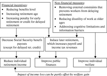
Based on our model and previous discussion, we would recommend instead the use of what we dub a ‘combination approach’. The key elements of that strategy are summarized in Figure 3. The basic idea is to make the financial incentives to delay retirement more effective by combining them with a set of non-financial measures. Broadly defined, these include removing external constraints that prevent workers from delaying retirement, reducing the disutility of work at older ages, and addressing cognitive limitations (or information barriers) that can result in earlier-than-optimal retirement decisions.
The combination approach

The combination approach is interesting for several reasons. First, it benefits public finances because more people would delay retirement and pay additional taxes. Second, the non-financial measures listed in Figure 3 have the added benefit of potentially improving individuals' welfare. This gain can help offset part of the loss that the worker suffers through the reduction in benefits. This was illustrated in Section 3 when we considered the case of an increase in E[τexo]. The gain could even be greater if, as suggested in Calvo (Reference Calvo2006), working longer can improve the individual's well-being for reasons other than financial. In addition, by seeking to improve the ability to work longer, some policies may have the added benefit of enhancing welfare aspects that were not captured in our model (e.g. utility from health). Third, it recognizes the heterogeneity in workers' characteristics and that a multifaceted approach can be more adequate in that context. For example, financial incentives cannot affect much the retirement timing of the constrained worker, but removing constraints can. By contrast, the weakly constrained worker is not usually forced to retire early and lowering the disutility cost of work is more likely to affect his retirement behavior.
Our suggested approach will be more effective if the non-financial measures listed in Figure 3 can be implemented at low cost. Recent developments in the UK provide a concrete example of the combination approach, and they may help us gain a better understanding of this aspect of the problem. In 2002, the UK setup a Pensions Commission to tackle the country's numerous pension issues. After undergoing a broad consultation process, the Pension Commission issued its final recommendations in 2006. Most of these proposals were adopted by the government in its White Paper, notably an increase in the State Pension Age (SPA) from 65 to 68.Footnote 9 The White Paper acknowledges that to be most beneficial for public expenditures, this modification should ideally be accompanied by an increase in actual retirement ages. Otherwise, pension costs may simply be shifted to other programs such as disability and unemployment.
Accordingly, a substantial portion of the White Paper is devoted to encouraging and enabling extended working lives. Most of the suggested measures can be viewed as applications of the broad strategies that we outlined in Figure 3. Financial incentives to work longer include a more generous delayed retirement provision with the possibility of a lump sum and the opportunity to receive a pension while working. In terms of removing external constraints to delayed retirement, they propose an age discrimination law, support for returning to work, and promoting age diversity in the workplace.
The disutility cost of working at older ages can be reduced by some of these measures and by the government's stated intention to work with employers to facilitate flexible work and phased retirement. Finally, an interesting aspect of the proposals is to correct the ‘behavioral mistakes’ that people make when they retire too early. For instance, better information would be provided about life expectancy and the link between work and retirement income. They also plan to pilot a program of face-to-face guidance sessions to help older workers understand their options in terms of work, training, and retirement.
5 Conclusion
Several studies (e.g. Butrica, Smith, and Steuerle, Reference Butrica, Smith and Steuerle2006) have documented that assuming later retirement can significantly improve measures of retirement income and public pensions funding. However, the literature has largely overlooked the impact that working longer has on welfare. We investigate the value of delaying retirement by introducing a life-cycle model where working is costly (in terms of lost leisure) and where retirement results from a combination of endogenous and exogenous factors. With this utility-based perspective, we find that the benefits associated with retiring later are much more limited than those suggested by previous studies. As a result, we conclude that traditional pension analysis tools may not be adequate when it comes to evaluating the potential benefits associated with working longer. In particular, we identify two issues: the omitted cost problem and the overstatement of the retirement response.
As an application of our model, we suggest a different way to approach Social Security reform. Most of the policies evaluated in the previous literature are related to a change in Social Security's parameters (such as the NRA or the Earnings Test.) Given that these parameters are not the only determinant of retirement behavior, it can be useful to consider an alternative set of policies aimed at improving the willingness and ability to work at older ages. This approach has the double advantage of increasing tax revenues and reducing the individual's welfare loss. We describe a concrete example of that strategy in Section 4 with the case of the recent UK pension reform.
In future research, our model could be extended in several directions. Borrowing constraints could be added and alternative specifications for work and leisure could be considered, such as the ones described in related works by Benítez-Silva and Heiland (Reference Benítez-Silva and Heiland2006), Gustman and Steinmeier (Reference Gustman and Steinmeier2005), and French (Reference French2005). We could also gain better estimates for the model's inputs through empirical work. Finally, we end by suggesting that our model be used to shed some new light on existing retirement puzzles. For instance, our finding that small changes around an endogenous retirement date have relatively little impact on welfare might help explain the clustering in retirement ages at 62 and 65 in the United States.
Appendix
(A) Solution to the optimization problem
Proposition 1 below gives the solution to our optimization problem in (5). Before presenting that solution, it will be helpful to introduce some notation and functions. We use the state-price density function

where we assumed that the exogenous retirement shocks are not priced by the market.
The technical term for our retirement date τ is a ‘stopping time’. We denote by S the set of all the possible stopping times in the problem. When we use τ as a subscript in a function, it indicates that the expectation in that function is taken according to the distribution of τ. For instance, for a given τ∊S, we define the functions A τ(t) and Y τ(t) as

and
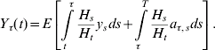
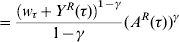
We sometimes use the shorthand notation A τ≡A τ(0) and Y τ≡Y τ(0) at time 0. Similarly, we have A R(τ)≡A τ(τ) and Y R(τ)≡Y τ(τ) at the time of retirement. With this notation, it is straightforward to show that given (1) and (3), the solution to the post-retirement optimization problem is
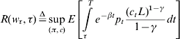
To solve our problem, we use the dual approach suggested in Karatzas and Wang (Reference Karatzas and Wang2000) and introduce a variable λ>0. For that purpose, it will be useful to introduce some additional functions. Letting λt≡λH t, for a given λ>0 and τ∊S, we define the functions

and

We also introduce the inverse function λ(W t,t) which satisfies

Proposition 1 below uses these functions to give the solution to our optimization problem.
Proposition 1 Let u(c t,t), R(w τ,τ), H t, A τY τ,  ,
 , and λ(W t,t) be defined respectively by equations (1), (9), (6), (7), (8), (11), (12), and (13). If the retirement strategy τ* optimizes
 and λ* solves
 , then the solution to the optimization problem in (5) is given by

At time 0⩽t<τ, the optimal consumption and investment in the risky asset are given respectively by

Proof. To prove this proposition, we use the dual approach suggested by Karatzas and Wang (Reference Karatzas and Wang2000) for an optimization problem with a discretionary stopping time. We extend their results to take into account factors such as labor income, pensions, and exogenous retirement shocks. The complete proof for this proposition is fairly lengthy and we present it in a supplement to this paper.□
The retirement criteria in Proposition 1 can be interpreted as follows. If the individual is still working at time t, he will retire at that time if this decision optimizes the function  or if he is forced to retire, i.e. if τexo=t. This can seem pretty abstract at first, but we can show that this criterion is in fact quite intuitive. To see this, suppose that at time t the individual is considering two options: retiring immediately or continuing to work according to a ‘schedule’ τ. Working longer would increase his income by
 and also increase the function A by
 .
We can estimate the effect that these changes have on welfare by taking the partial derivatives of V(w) with respect to Y τ and A τ The marginal benefit (MB) from the additional income would be MB=λtΔY and the marginal cost (MC) from the lost leisure would be MC=(γ/(γ−1))λt1−1/γΔA. Note that MB, MC, and MB−MC all increase with λt, and thus they decrease with total wealth. With this notation, it is straightforward to show that optimizing  over τ∊S is equivalent to the strategy ‘delay retirement as long as MB>MC and retire when MB=MC’.
Alternatively, the criteria ‘retire when MB=MC’ can be rewritten as ‘retire when λt decreases to [(γ−1)ΔY/γΔA]−γ’. Given that λt=λ*H t, the worker will be closer to retirement when H t is low, i.e. when investments perform well. This will also be the case if λ* (the initial marginal utility of wealth) is low, which happens when initial wealth and pensions are relatively high, or when life expectancy is shorter. In addition, we can predict that the worker will be closer to retirement when ΔY is low or ΔA is high. A quick examination of our formulas for ΔY and ΔA shows that this will be the case when (1) labor income is not much higher than pension income, (2) there is a small increase in pensions for delaying retirement, and (3) the utility of leisure is relatively high.
(B) Numerical evaluation
To solve the problem numerically, we discretize the interval [0,T] into small intervals of length Δt. We index these intervals by i=0,1, …, T/Δt and project the values of H iΔt on a binomial or trinomial tree.Footnote 10 Accordingly, we can obtain some simple recursive equations for all the formulas in Proposition 1 by using the following assumptions: (1) the endogenous retirement decision can only be made at the beginning of each of the periods, (2) if there is an exogenous retirement shock in period i, the worker will retire at the end of that period, and (3) the functions p s and y s are constant over each period i. We list the resulting recursive equations in a supplement to this paper.
To solve for λ*, we use the bisection method. First, we fix a value of λ and project λt=λH t for each of the tree's periods and nodes. We then solve for the optimal stopping time  (see explanation below). With determined, we can compute
 ,
 , and
 . We test whether is close enough to the initial wealth w. If not, we adjust λ using the bisection method's rule and repeat the process until convergence.
For a given λ, we can solve for the optimal stopping time by moving backwards in the tree. We start by assuming that the worker must be retired by period M. Moving back one period to M−1, there are only two possible scenarios for the stopping time τ: retiring immediately or working for the next period and then retiring. It is straightforward to compute  recursively for these two scenarios and determine whether it is optimal to retire for each of the possible values of λt. Moving back to period M−2, we consider the following options for τ: retiring immediately or working in period M−2 and using the optimal work/retirement strategy for period M−1. Given that we have already derived the optimal work/retirement strategy in period M−1, it is easy to compute
 recursively for each scenario. We can then determine whether it is optimal to work or retire for each of the nodes. We repeat the same procedure by moving backwards in the tree until we reach period 0.
(C) Assumptions for numerical example in Section 3
The illustrations in Section 3.2 were computed with the formulas in Proposition 1 and the following assumptions. (Note: All economic assumptions are expressed in real terms.) The worker is currently 55 years old and he can live up to 100 years old. His mortality table is constructed with unisex data from the year 2000 from the National Center for Health Statistics (NCHS). We assume that the worker can potentially work until age 75 and he is subject to an exogenous retirement shock distributed according to a Gompertz distribution with parameters m=11.9585 and b=3. With these assumptions, the expected time until the worker is forced to retire is E[τexo]=65.5−55=10.5. The probability of still being able to work in t years is given by exp(e −m/b(1−e t/b)). Note that the Gompertz distribution is commonly used to represent mortality and we chose it because it models the ‘exogenous force of retirement’ as increasing with age.
The risk-free rate is r=2%, the expected return of the risky asset is μ=6%, and its standard deviation is σ=20%. In terms of preferences, we set β=4% and γ=3. For L, the parameter representing the utility of leisure, we assume that the weakly constrained worker values leisure highly (L=2.50) and that the constrained worker values leisure much less (L=1.25).
The initial income is y0=$25,000 and we assume that it grows at a rate of g=0%. This income is subject to income taxes (according to the tax rates in the 2005 IRS 1040 form) and to a 7.65% Social Security tax rate (for both the employee and the employer). The initial savings are w=$100,000. At retirement, the individual derives income from his savings and from a Social Security pension. The benefit is determined according to the formula for the 2006 primary insurance amount (PIA). In that formula, we simplify the calculation of the average indexed monthly earnings (AIME) and assume that the AIME is equal to y 0. Initially, we set the NRA to 65.5 years old. (This is actually the NRA for the cohort born in 1940.) The worker can retire before that age, but his pension will be reduced accordingly. This reduction is 0.555% per month for the first 36 months and 0.416% per month thereafter. The earliest age to receive the Social Security pension is 62. (If the worker retires before age 62, we assume that he will claim his Social Security pension at 62. Note that we impose a minimum requirement on wealth for retiring before age 62). If retirement is delayed past the NRA, the benefit is increased by 7.5% every year up to age 70.