

Single-case experimental designs (SCEDs) are strategies capable of meeting criteria for experimental quality (Smith, Reference Smith2012) and useful for identifying evidence-based practices (Schlosser, Reference Schlosser2009). SCEDs entail the study of a single participant in different conditions, manipulated by the researcher and gathering repeated measurements in each of these conditions. However, it should be noted that most SCED studies involve studying separately more than one participant (Shadish & Sullivan, Reference Shadish and Sullivan2011; Smith, Reference Smith2012), especially in relation to the importance of replicating the effects of the intervention (Kratochwill et al., Reference Kratochwill, Hitchcock, Horner, Levin, Odom, Rindskopf and Shadish2010). The data obtained are represented graphically and the assessment of the difference between conditions has traditionally been performed visually (e.g., Parker & Brossart, Reference Parker and Brossart2003; Smith, Reference Smith2012). The continued use of visual analysis is likely due to the amount of data features that need to be taken into account (Kratochwill et al., Reference Kratochwill, Hitchcock, Horner, Levin, Odom, Rindskopf and Shadish2010; Parker, Cryer, & Byrns, Reference Parker, Cryer and Byrns2006) and the need to understand well the behavioural process (Fahmie & Hanley, Reference Fahmie and Hanley2008). However, statistical analyses are already part of neuropsychological rehabilitation SCED studies (Perdices & Tate, Reference Perdices and Tate2009), probably in relation to the evidence of insufficient interrater agreement between visual analysts (Ninci, Vannest, Willson, & Zhang, Reference Ninci, Vannest, Willson and Zhang2015), the need to take into account spontaneous improvement during the baseline and/or excessive variability (Kazdin, Reference Kazdin1978), and the importance of objectively documenting intervention effectiveness and making SCD studies eligible for meta-analyses (Jenson, Clark, Kircher, & Kristjansson, Reference Jenson, Clark, Kircher and Kristjansson2007).
In order to illustrate the application and interpretation of several analytical techniques, we re-analyse the data from two SCEDs studies, including a variety of data features, such as baseline stability versus variability versus spontaneous improvement. We show that it is possible to express the results in the same metric as the outcome variable, as a percentage, or in standard deviations (SD). Additionally, we will also rely heavily on visual representations of the data to enhance the interpretation of the numerical results. Finally, we provide references to analytical techniques not covered here. (Note that the Special Issue in which the current text is included also covers structured visual analysis and the meta-analytical integration of individual studies).
A Comment on Terminology
Rationale for the comment on terminology
We consider that the readers of Brain Impairment are likely to be familiar with the Risk of Bias in N-of-1 Trials (RoBiNT) methodological quality scale (Tate et al., Reference Tate, Perdices, Rosenkoetter, Wakima, Godbee, Togher and McDonald2013) and with the fact that in its data analysis item the terms ‘statistical and quasi-statistical’ techniques are used. In that sense, we would like to provide a brief discussion of these terms and the ones we used throughout the paper (i.e., descriptive and inferential).
Available examples
In the expanded manual of the RoBiNT scale (Tate et al., Reference Tate, Rosenkoetter, Wakim, Sigmundsdottir, Doubleday, Togher and Perdices2015), the examples of statistical analyses include randomisation tests and effect size indices, whereas the examples of quasi-statistical techniques include the 2 SD method and celebration (trend) lines with Bayesian probability analysis. In relation to these examples, trend lines and the 2 SD method are referred to as ‘visual aids’ (rather than quasi-statistical techniques) by Fisher, Kelley, & Lomas (Reference Fisher, Kelley and Lomas2003), who propose one of the supported (Young & Daly, Reference Young and Daly2016) methods for performing structured visual analysis. Additionally, the 2 SD bands are based on the normal probability model and are part of ‘statistical process control’ (Callahan & Barisa, Reference Callahan and Barisa2005), which suggests that they can be called a ‘statistical technique’. Analogously, split-middle trend line has been used with binomial (rather than Bayesian) probability analysis (Crosbie, Reference Crosbie1987) and referring to a probability model indicates that such a use of the trend line is ‘statistical’ in nature. Finally, regarding non-overlap indices, there have been arguments for considering them as ‘effect size’ measures (Carter, Reference Carter2013) and thus ‘statistical’ according to the RoBiNT scale or for including them in the steps outlined for visual analysis (Lane & Gast, Reference Lane and Gast2014), which can be interpreted as non-overlap indices being part of ‘systematic visual analysis’ in terms of the RoBiNT scale.
Terminology in the current text
According to the distinction we establish here, ‘statistical techniques’ are the ones that are based on statistical theory and make possible obtaining confidence intervals and p values on the basis of the knowledge of the sampling distribution of the statistic, whereas ‘quasi-statistical techniques’ are the descriptive measures or ad hoc quantifications for which the precision of the quantifications cannot be assessed, as there is no expression available for estimating their standard error.
In summary, in relation to the terms used in the RoBiNT scale, we do not claim that our distinction is flawless, because it can also be argued that according to our definition ‘statistical techniques’ refer to inferential statistics, whereas ‘quasi-statistical techniques’ refer to descriptive statistics, with both being ‘statistical’. Moreover, an ‘effect size’ may not be clearly classifiable, considering that the definition and facets of effect size provided by Kelly and Preacher (Reference Kelley and Preacher2012) potentially includes a variety of descriptive (quasi-statistical) indices, but these authors also stress the importance of having appropriate indicators of measurement error or uncertainty and reporting confidence intervals (as for statistical techniques). In any case, we remark that the use of terms such as ‘visual aid’, ‘effect size’, ‘quasi-statistical techniques’ and ‘statistical analysis’ may not have a universally accepted meaning and it is therefore necessary that in each report it is specified exactly what is being done with the data and that a justification is provided.
Description of a Selection of Techniques
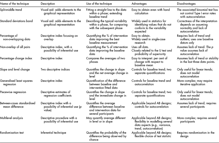
Table 1 includes a simplified description of several analytical techniques applicable to SCED data, specifically focusing on the techniques mentioned in the current text. Nevertheless, it is necessary to underscore that we do not present a comprehensive list of techniques and we do not claim that the techniques illustrated are the optimal ones for all data sets. Different applied researchers, methodologists and statisticians may choose different analytical techniques as optimal ones. We suggest that the reader interested in further options should consult the list available in the Appendix to the SCRIBE explanation and elaboration document (Tate et al., Reference Tate, Perdices, Rosenkoetter, McDonald, Togher, Shadish and Vohra2016); more references for an in-depth study of the analytical alternatives are provided in the ‘Analytical Challenges and Recommendations’ section.
Summary of the Main Features of Several Analytical Techniques Applicable to Single-Case Experimental Designs Data

The reasons for choosing the techniques were to illustrate (a) the variety of data aspects modelled: level, trend, overlap, immediacy, all mentioned as relevant when performing visual analysis (Kratochwill et al., Reference Kratochwill, Hitchcock, Horner, Levin, Odom, Rindskopf and Shadish2010); (b) the variety of ways of estimating trend: ordinary least squares regression, split-middle, average of the differences between consecutive measurements and (c) the fact that both descriptive and inferential techniques can be used. In absence of a clearly stated expectation about whether the effect should be an immediate change in the average performance or a progressive or delayed change, we followed the idea (Manolov & Moeyaert, Reference Manolov and Moeyaert2017b) that the analytical technique can be chosen in such a way as to represent better the features of the data at hand. Therefore, for each example we further justify the choice of the techniques.
Quantifications of Overlap
Non-overlap of all pairs (NAP)
A technique that is not easily classifiable as quasi-statistical or statistical is NAP (Parker & Vannest, Reference Parker and Vannest2009). Given that the result is expressed as a percentage of non-overlap between conditions, NAP is apparently similar to the Percentage of non-overlapping data (PND; Scruggs & Matropieri, Reference Scruggs and Mastropieri2013) for which the sampling distribution is not known, but it is also possible to derive the standard error for NAP on the basis of its equivalence with the Mann–Whitney U test or the probability of superiority (Grissom & Kim, Reference Grissom and Kim2001). In the current text we focus on the descriptive (not inferential) use of NAP. The strengths of NAP are: (a) it uses all data unlike the PND, which is one of the reasons for its proposal; (b) it is not based on representing the data via a mean or a trend line; (c) under the assumption of independent data it is possible to obtain a p value; (d) among the techniques mentioned here, NAP, is the only one applicable to ordinal data and (e) it can be applied using a website http://www.singlecaseresearch.org/calculators/nap. As limitations, NAP does not control for baseline trend and does not quantify the amount of difference once complete non-overlap is achieved: it may present ceiling effects, not distinguishing between treatments with different degree of effectiveness.
Other non-overlap indices
Parker, Vannest, & Davis (Reference Parker, Vannest and Davis2011) compare several non-overlap measures and conclude that NAP is among the most powerful ones and it also yields similar results to other non-overlap indices. Non-overlap indices can be computed via https://jepusto.shinyapps.io/SCD-effect-sizes/, http://manolov.shinyapps.io/Overlap/ and http://ktarlow.com/stats/.
Quantifications of the Difference in Level
Percentage change index (PCI)
A numerical summary expressed as the average difference between conditions in relation to the baseline level has been named ‘mean baseline difference’ (Campbell & Herzinger, Reference Campbell, Herzinger and Gast2010), ‘per cent reduction’ (Olive & Smith, Reference Olive and Smith2005) or ‘percentage change’ index (Pustejovsky, Reference Pustejovsky2015). The mean baseline difference usually refers to the difference between the intervention phase mean and the baseline phase mean, expressed as a percentage of the baseline phase mean. The PCI is usually computed following the same logic, but using only the last three baseline measurements and the last three intervention phase measurements. For the latter case, Hershberger, Wallace, Green, & Marquis (Reference Hershberger, Wallace, Green, Marquis and Hoyle1999) present an expression for estimating its variance. According to whether such an expression is accepted as valid or not, the PCI could be considered a statistical or quasi-statistical technique. It is mainly useful when a mean line represents well the data (i.e., there are no trends and the variability is not excessive) and when the baseline data are not all equal to zero (as it would impede obtaining a quantification). The PCI can be computed using https://manolov.shinyapps.io/Change/.
Between-cases standardised mean difference (BC-SMD)
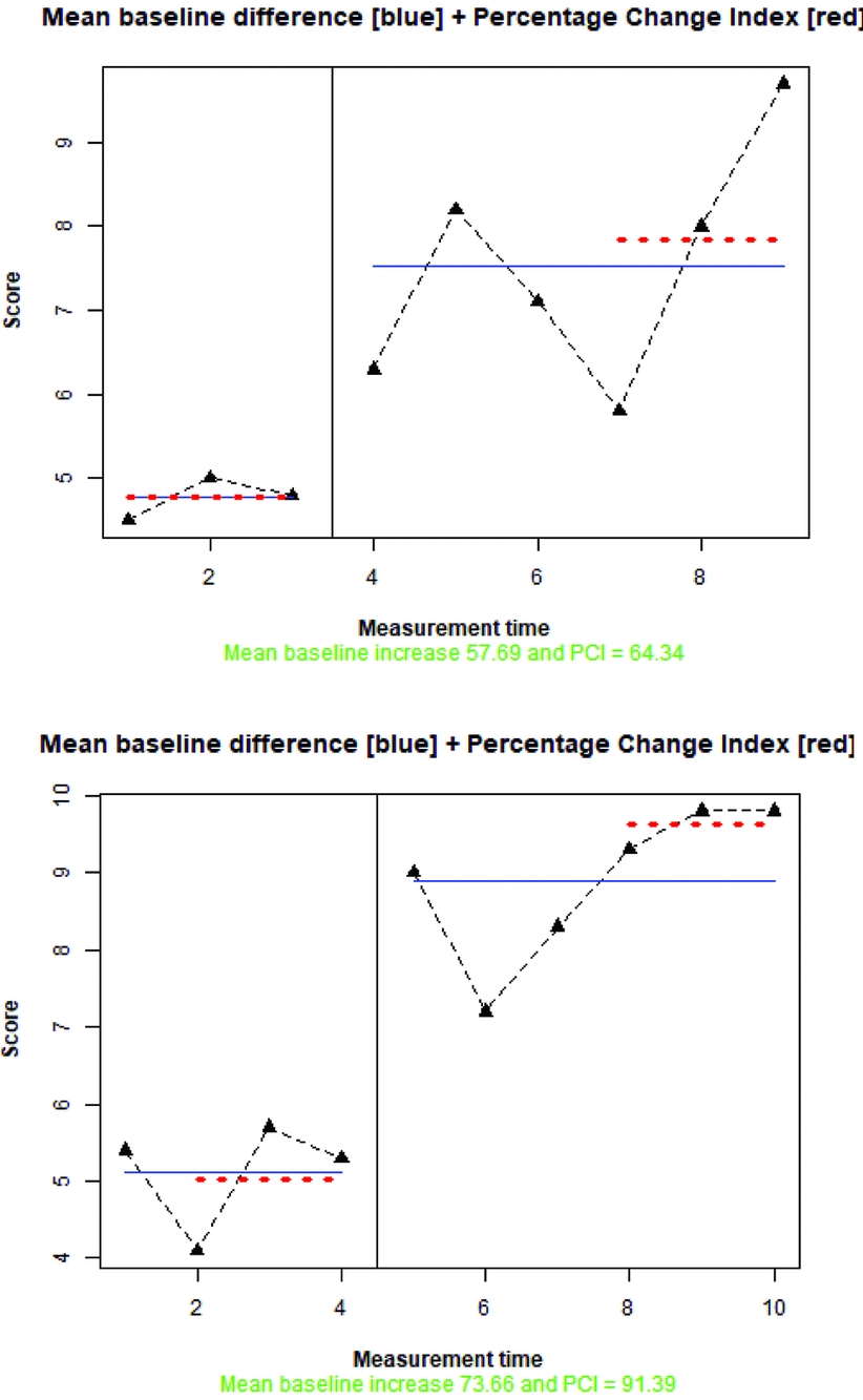
A statistical technique developed specifically for SCEDs is the BC-SMD or d-statistic (Shadish, Hedges, & Pustejovsky, Reference Shadish, Hedges and Pustejovsky2014). The BC-SMD was developed to provide a quantification comparable to the ones from group-comparison studies, making possible the meta-analytical integration of results from different designs, given that the within-case SMD does not allow for that (Beretvas & Chung, Reference Beretvas and Chung2008). Other strengths of the BC-SMD include taking autocorrelation into account, the attainment of an overall quantification of intervention effect across cases, the comparability across studies measuring outcomes in different measurement units, and the possibility to obtain confidence intervals and to use inverse variance weight in meta-analysis. Moreover, note that the BC-SMD takes into account both the variability of the data within a case and between-cases, whereas the PCI is based only on quantifications of the average level. The BC-SMD can be applied via the website https://jepusto.shinyapps.io/scdhlm/. The BC-SMD is only applicable when there are several cases in the same study and it is also mainly applicable to stable data (although detrending is possible, Shadish et al., Reference Shadish, Hedges and Pustejovsky2014) and when the intervention effect is an immediate change in level. In order to illustrate this assumption, we refer to two data sets presented later in the text. For instance, the data depicted on the upper panel of Figure 1 can be considered to represent stable data (no trend in the baseline or in the intervention phase) and the intervention effect can be understood as immediateFootnote 1 , because difference between the two conditions takes place already in the beginning of the intervention phase. These data would fit the assumptions of the BC-SMD. As a different example, Figure 2 also shows an immediate difference, but the data is not stable and the trends are not comparable (i.e., there is both a change in level and in slope). These data would not fit the assumptions of the BC-SMD. Additional assumptions include the homogeneity of the effect across cases, the normal distribution of within-case errors and the autocorrelation process being first-order autoregressive, although the estimates of effect are robust to violating these assumptions, which are mostly important for its small-sample correction (Valentine, Tanner-Smith, & Pustejovsky, Reference Valentine, Tanner-Smith and Pustejovsky2016).
Application of the percentage change index (PCI, computed on the last three measurements per phase; dotted horizontal line) and the mean baseline difference (computed on all measurements; solid horizontal line). The upper panel refers to Samantha and the lower panel to Thomas; data gathered by Douglas et al. (Reference Douglas, Knox, De Maio and Bridge2014). Graphs obtained from https://manolov.shinyapps.ioChange/. For each of the two plots, the data to the left of the vertical line belong to the baseline (A) phase and the data to the right belong to the intervention (B) phase.

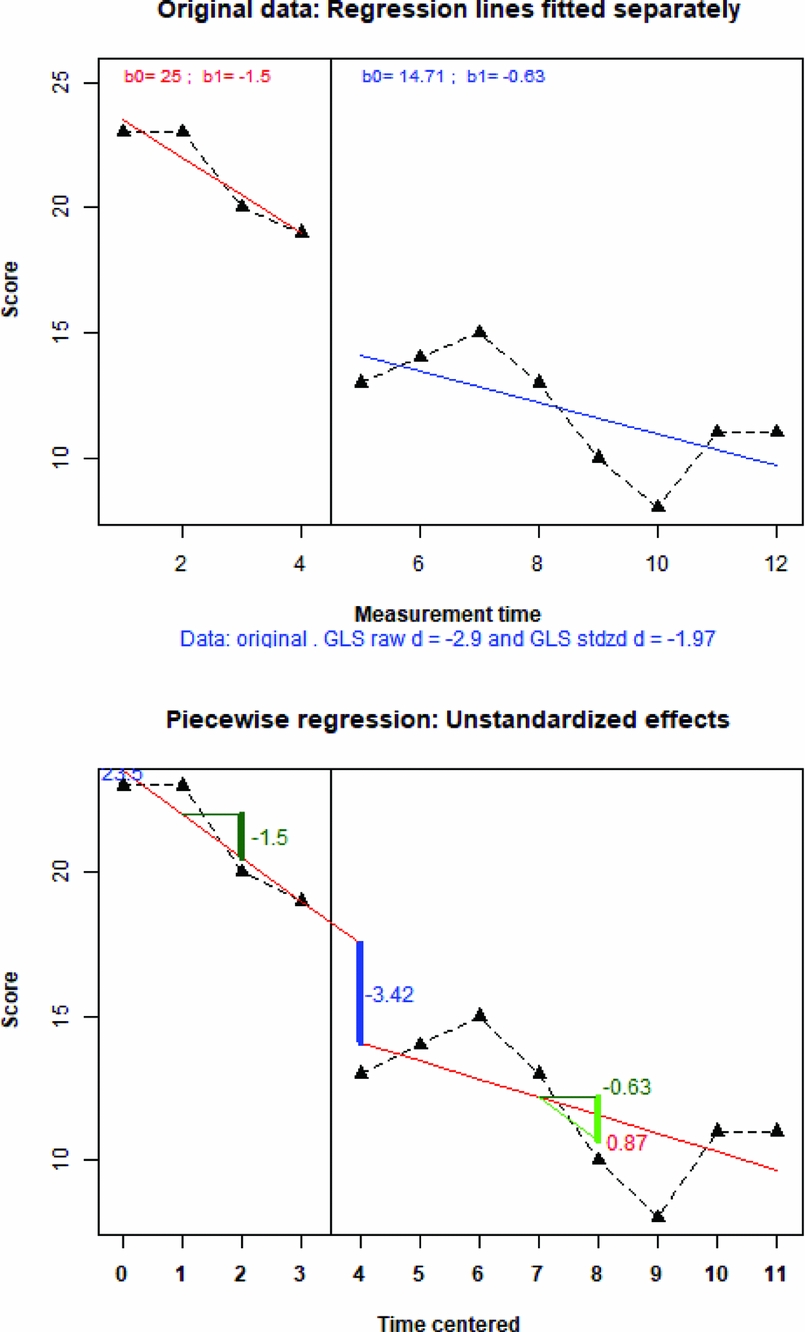
Application of Piecewise regression (upper panel) and generalised least squares regression (GLS; lower panel) to the data gathered by Ownsworth et al. (Reference Ownsworth, Fleming, Desbois, Strong and Kuipers2006) on the frequency of errors in a cooking task. Graphs obtained from https://manolov.shinyapps.io/Regression/. For each of the two plots, the data to the left of the vertical line belong to the baseline (A) phase, and the data to the right belong to the intervention (B) phase. On the upper panel, for both phases, b0 denotes the within-phase intercept and b1 the within-phase slope.

Quantifications of the Differences in Level and in Slope
Slope and level change (SLC)
The SLC (Solanas, Manolov, & Onghena, Reference Solanas, Manolov and Onghena2010) is a descriptive technique not based on statistical theory. It entails: (1) quantifying baseline trend: how much spontaneous improvement is there per measurement occasion; (2) removing baseline trend from the baseline and intervention phase data: how would the data look like without the spontaneous improvement; (3) quantifying the amount of change in slope: to what extent is the progressive change in the intervention greater than the spontaneous change in the baseline and (4) quantifying the amount of net change in level: apart from the difference in trends, how much is the average difference between conditions. The SLC presents the following strengths: (a) it provides a quantification in the same measurement units as the outcome variable, which aids the interpretation in meaningful terms; (b) it allows taking into account linear baseline trend; (c) it quantifies change in slope (as the average change between consecutive measurements) and change in level (as a mean difference, once change in slope is taken into account) separately, which is the reason for its development, following the recommendation by Beretvas and Chung (Reference Beretvas and Chung2008); (d) its descriptive purpose entails that there are no assumptions regarding normality or lack of serial dependence; and (e) it can be applied using a website (http://manolov.shinyapps.io/Change/) which offers both numerical and graphical output. Among the limitations of the SLC, its quantifications are: (a) mostly meaningful when the data are stable or present linear trends; (b) not comparable across studies using different outcome variables and (c) not accompanied by indicators of precision such as confidence intervals.
Regression analyses
Piecewise regression (Center, Skiba, & Casey, Reference Center, Skiba and Casey1985–1986) offers the possibility to quantify separately the immediate effect of the intervention and the difference in slopes. The descriptive quantification of these data aspects does not require the parametric assumptions of regression analysis (normally, homogeneously and independently distributed residual), but the interpretation of their statistical significance is subjected to these assumptions. Note that Piecewise regression can be applied beyond AB-comparisons, as described in Moeyaert, Ugille, Ferron, Beretvas, & Van Den Noortgate (Reference Moeyaert, Ugille, Ferron, Beretvas and Van Den Noortgate2014b). In order to deal with autocorrelation, a regression-based analysis using generalised least squares estimation (GLS; Swaminathan, Rogers, Horner, Sugai, & Smolkowski, Reference Swaminathan, Rogers, Horner, Sugai and Smolkowski2014) was proposed. In GLS, an overall quantification of the difference between conditions is obtained after fitting trend lines separately to the baseline and intervention phase data; this quantification can be raw or standardised. These regression techniques are mainly applicable when the data in the two conditions compared are either stable or exhibiting an approximately linear trend. Moreover, the testsFootnote 2 for autocorrelation performed by the GLS require that the autocorrelation and the error variances are homogeneous across the conditions being compared. Both regression approaches can be applied via a website https://manolov.shinyapps.io/Regression/.
Other Analytical Options
The list of techniques presented is not comprehensive. Further options for statistical analysis include: (a) randomisation tests (Heyvaert & Onghena, Reference Heyvaert and Onghena2014), if randomisation is present in the design and a p value is desired; (b) log response ratio measures (Pustejovsky, Reference Pustejovsky2015) for data gathered via direct observation and interpretations desired in terms of percentage change; and (c) multilevel models (Moeyaert, Ferron, Beretvas, & Van Den Noortgate, Reference Moeyaert, Ferron, Beretvas and Van Den Noortgate2014a), if data are available for several participants and average estimates of effect are of interest, besides quantifying the amount of variation across individuals.
Illustrations in the Context of Brain Impairment
First Example: Stable Baselines and Replication
Data
Douglas, Knox, De Maio, & Bridge (Reference Douglas, Knox, De Maio and Bridge2014) report a study on two participants (Samantha and Thomas) with traumatic brain injury, treated with Communication-specific coping intervention. The design is referred to as an ‘A–B–A design with follow-up using multiple probes’ (Douglas et al., Reference Douglas, Knox, De Maio and Bridge2014, p. 194). Nevertheless, there are three reasons for assuming that the design is probably better conceptualised as an AB design with a follow-up: (a) the time intervals in the last phase are farther apart in time, (b) the intervention is not strictly speaking withdrawable and (c) the performance is not expected (or desired) to revert to the initial baseline levels. Among the outcomes of interest, quantifications were obtained using a visual analogue scale, ranging from 0 to 10 cm with greater values representing better communicative performance.
Visual inspection
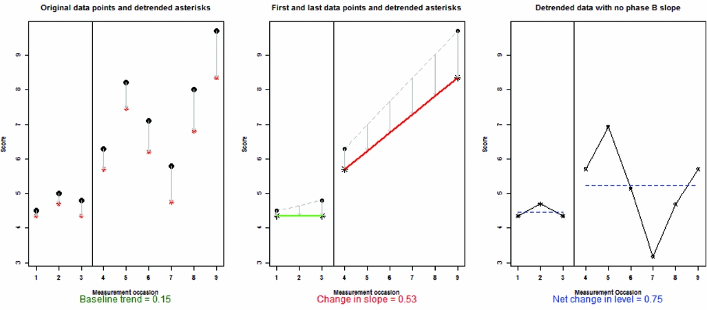
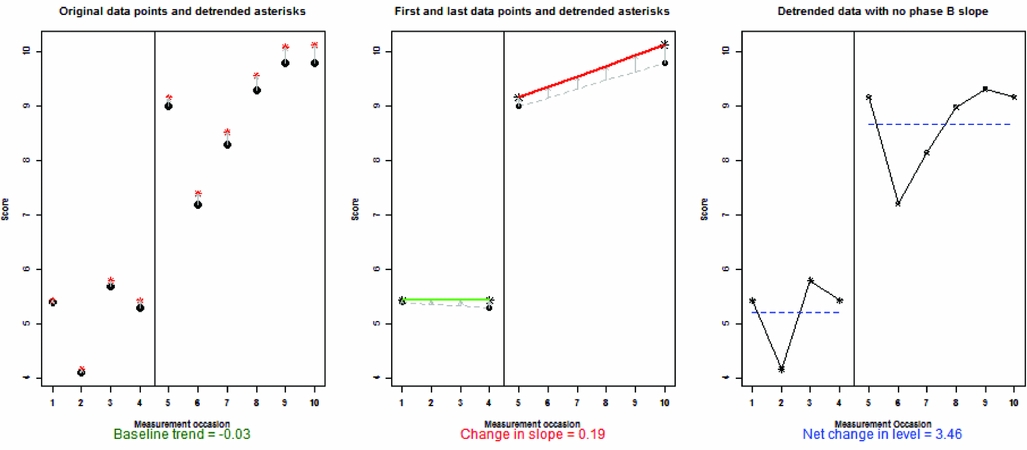
Figures 3 and 4 present, in their left panels and with filled black dots, the original data for Samantha and Thomas, respectively. The asterisks in the left panels show how the data look like when removing baseline trend, which is done in the context of the SLC in order to represent how much of an improvement is there with the introduction of the intervention, beyond the improvement already taking place during the baseline. The middle panels of Figures 3 and 4, show the trends in the original data (thin-dashed lines) and the trends in the transformed data (thick solid lines). Given that the slope of baseline trend is close to zero (i.e., almost flat), the baselines are relatively stable. Therefore, detrending does not affect greatly the values. The intervention phase measurements are more variable and show certain increasing trend, indicative of change in slope (which can also be called change in trend). The right panels of Figures 3 and 4 show the net (pure) change in level, after controlling for the intervention phase trend. The amount of vertical distance between the dashed lines representing the within-phase means is indicative of a change in level.
Application of the percentage change index to the data gathered by Douglas et al. (Reference Douglas, Knox, De Maio and Bridge2014): participant called Samantha. Graphs obtained from https://manolov.shinyapps.io/Change/. For each of the three plots, the data to the left of the vertical line belong to the baseline (A) phase and the data to the right belong to the intervention (B) phase.

Application of the percentage change index to the data gathered by Douglas et al. (Reference Douglas, Knox, De Maio and Bridge2014): participant called Thomas. Graphs obtained from https://manolov.shinyapps.io/Change/. For each of the three plots, the data to the left of the vertical line belong to the baseline (A) phase and the data to the right belong to the intervention (B) phase.

Justification of the choice of the analytical techniques
The absence of clear baseline trend makes applicable the PCI and the BC-SMD, as both compare mean levels. The possible presence of intervention phase trend makes useful the application of the SLC in order to quantify the progressive change (i.e., the slope change). Moreover, the SLC is more meaningful when the baseline data are well represented by the trend line. We did not use NAP, for instance, given that the result would be 100% in both cases, therefore, not distinguishing between the different distances between the baseline and intervention phase measurements for the two participants.
Slope and level change
The application of the SLC to Samantha's data (Figure 3) shows that there is a slightly improving baseline trend (.15), and that beyond this initial trend, after the intervention there is an average increase of the communication score of .53 per measurement occasion (i.e., a gradual 1 cm increase for each two sessions). Additionally, there is an average difference increase in level of .75 cm in the intervention phase. Considering that the scale ranges from 0 to 10 cm, that baseline values are around 4–5 cm, and that by the end of the intervention Samantha's scores are near 9 cm, the improvement seems relevant.
For Thomas (Figure 4), the baseline data are practically stable (trend = −.03) and the average gradual increase appears to be quantitatively small (.19) due to the fact that the there is a marked decrease from the first to the second measurement in the intervention phase. However, from the second intervention phase data point onwards a marked gradual improvement is visually clear. In that sense, we recommend using visual analysis to help interpreting the quantitative results. The net average difference is considerable: almost 3.5 cm, with the final two measurements being close to 10 cm, indicative of the effectiveness of the intervention. Note that in this example the interpretability is not necessarily aided by the fact that the SLC summarises the results in the same measurement units as the outcome variable, because the centimetres of the visual analogue scale are not as readily interpreted as would be, for instance, the number of errors in a speech. For that reason, we offer further quantifications.
Percentage change index
Figure 1 focuses on the within-phase means, with a solid horizontal line representing the mean of all the measurements in each phase and the dashed horizontal line representing the mean of only the last three measurements per phase. For Samantha (upper panel of Figure 1), the percentage increase for Samantha is approximately 60% regardless of whether all data or only the last three measurements per phase are considered. For Thomas (Figure 1; lower panel), PCI = 73.66% considering all data and 91.39% focusing on the last three data points per condition. For both participants, NAP = 100%. However, as shown using the PCI, for Thomas the difference between conditions is larger than for Samantha, despite the fact that there is complete non-overlap for both, illustrating one of NAP's limitations.
Between-cases standardised mean difference
Apart from obtaining separate quantifications for each participant, another analytical option would be to obtain an overall quantification computing the BC-SMD. According to Zelinsky and Shadish (Reference Zelinsky and Shadish2016, p. 5) ‘one case allows computing the numerator of d, two cases allow computing the denominator, and three cases are needed to compute the standard error of d’ and thus we would obtain d = 3.51, which can be interpreted as the communication score being, on average for both participants, three and a half SD better during the intervention than before. On the basis of the graphical representationFootnote 3 that can be obtained from https://jepusto.shinyapps.io/scdhlm/, it can be visually assessed to what extent the effect can be considered homogeneous for both participants. Additionally, the aforementioned website provides the standard error (SE = 1.26), despite having only two cases, and a 95% confidence interval ranging from 1.65 to 6.16 and illustrating the low precision of the estimate. Nevertheless, Valentine et al. (Reference Valentine, Tanner-Smith and Pustejovsky2016) recommend applying the BC-SMD when there is a minimum of three cases. Thus, the result of d and especially its standard error reported should be interpreted with caution.
Overall assessment of intervention effectiveness
All the quantifications reflect the effectiveness of the intervention. Beyond the current (quasi)statistical analyses, the qualitative feedback provided by both participants and reported in Douglas et al. (Reference Douglas, Knox, De Maio and Bridge2014) is crucial for a comprehensive assessment of intervention effectiveness. In general, the numerical results provided here agree with Douglas et al.’s (Reference Douglas, Knox, De Maio and Bridge2014, p. 199) conclusion of ‘clinically significant improvements on expression and comprehension discourse tasks in participants’.
Second Example: Spontaneous Improvement and Unstable Baseline
Data
Ownsworth, Fleming, Desbois, Strong, & Kuipers (Reference Ownsworth, Fleming, Desbois, Strong and Kuipers2006) report a study on a participant with traumatic brain injury, presenting long-term awareness deficits and treated with a metacognitive contextual intervention. The outcomes included the numbers of errors in a cooking task (AB plus maintenance design) and in volunteering work (AB design), with lower values being more desirable.
Cooking task: visual inspection and justification of the choice of the analytical techniques
For the cooking task, visually there is a clear improving baseline trend. Therefore, this trend has to be taken into account when performing the analysis, in order to explore to what extent the intervention exceeds the spontaneous improvement. In that sense, the SLC is applicable to these data, but we want to illustrate further analytical options here: Piecewise and GLS regression. Both analytical options fit trend lines separately to each phase and in case the serial dependence is not statistically significant (and GLS does not lead to transforming the data) these trend lines are the same; that is, Piecewise and GLS yield identical resultsFootnote 4 . What is different is the focus of the analysis. In Piecewise regression the main quantifications are the immediate change (difference between the last predicted baseline measurement and the first predicted intervention phase measurement) and the change in slope (difference between the slopes of the trend lines). In GLS the baseline trend line is extrapolated into the intervention phase and is compared to the trend line fitted to the intervention phase data; a comparison between the two sets of predicted data points is performed.
Regarding alternative analytical approaches, the PCI is not meaningfully applicable here, given that mean differences are less informative when trend is present in both phases. NAP is also not appropriate, because it does not control for baseline trend.
Cooking task: regression analyses
According to Piecewise regression (see Figure 2; upper panel), the initial baseline level is 23.5 and, more importantly, baseline trend is equal to −1.5 (i.e., there are three errors less every two measurement occasions). After the intervention, Piecewise regression indicates an immediate decrease of 3.4 errors, but the improving trend is not as steep as in the baseline (−.87, which is .63 less than −1.5). According to GLS, the overall average difference, considering the different levels (intercepts by b1) and slopes (denoted by b0), would be a reduction of almost three errors as indicated in the foot of Figure 2 (lower panel). Therefore, both analytical options suggest a considerable reduction in the target behaviour, beyond the spontaneous improvement.
Volunteering work: visual inspection, justification of the choice of the analytical techniques, and numerical results
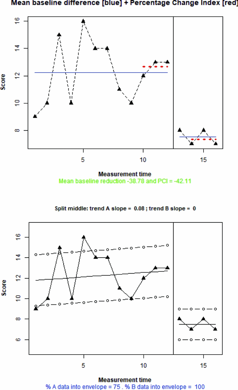
For volunteering work, the baseline data are more variable and not readily represented by a mean line (see the solid horizontal line in the upper panel of Figure 5) or by a trend lineFootnote 5 (see the solid line in the lower panel of Figure 5). Therefore, the application of the SLC and regression analysis is less justified. The PCI, focusing on the last three measurements per phase, is more meaningful than the mean baseline difference, given that the last three measurements are better represented by their mean (dashed lines) than the whole of the baseline data (Figure 5, upper panel). The PCI indicates a reduction of more than 40%. NAP is also especially useful for the volunteering work data, given that it does not require the data to be summarised by a mean or a trend line; NAP = 100%. Additionally, the assessment of trend stability (Lane & Gast, Reference Lane and Gast2014, using split middle trend ± 20% within-phase median; Figure 5, lower panel) suggests that the performance became more stable after the intervention.
Upper panel obtained via https://manolov.shinyapps.io/Change: application of the percentage change index (PCI; based on the dotted horizontal line representing the mean of the last three measurements per phase) and the mean baseline difference (based on the solid horizontal line representing the phase means). Lower panel obtained via https://manolov.shinyapps.io/Overlap: trend stability envelope, with the solid line representing split-middle trend. Data gathered by Ownsworth et al. (Reference Ownsworth, Fleming, Desbois, Strong and Kuipers2006) on the frequency of errors in volunteering work. For each of the two plots, the data to the left of the vertical line belong to the baseline (A) phase and the data to the right belong to the intervention (B) phase.

Overall assessment of intervention effectiveness
Considering all numerical results, the intervention seems effective in reducing the frequency of errors. However, the global evaluation of the effectiveness of the intervention, as performed by Ownsworth et al. (Reference Ownsworth, Fleming, Desbois, Strong and Kuipers2006), also includes the assessment of awareness of deficits via a questionnaire and an interview, for which the results were not clinically significant. In that sense, the (quasi)statistical information obtained on directly observable behaviours is only part of the evidence when assessing intervention effectiveness.
Additional Remarks
Ideally, statistical analysis should focus on quantifying the type of change (in level, trend or variability) expected for the intervention. In absence of explicitly stated expectations, looking for a change in level (e.g., using BC-SMD, SLC, PCI) seems most parsimonious and we proceeded accordingly with the Douglas et al. (Reference Douglas, Knox, De Maio and Bridge2014) data. However, the obtained data pattern needs to be considered as well, which is why we took into account the spontaneous improvement and the variable baseline in the Ownsworth et al. (Reference Ownsworth, Fleming, Desbois, Strong and Kuipers2006) data when selecting the analytical techniques.
It has to be noted that we relied on descriptive measures in our analyses, given that p values are not readily interpretable in terms of population inference, because it is not justified in absence of random sampling and the articles whose data is re-analysed here did not sample the participants at random from a population of individuals with similar characteristics. Moreover, tentative causal inference on the basis of a randomisation test (Edgington & Onghena, Reference Edgington and Onghena2007) is not possible for the data re-analysed here, given the absence of random assignment of measurement times to conditions. Nevertheless, we encourage researchers to implement randomisation and replication to enhance internal and external validity (Kratochwill et al., Reference Kratochwill, Hitchcock, Horner, Levin, Odom, Rindskopf and Shadish2010; Tate et al., Reference Tate, Perdices, Rosenkoetter, Wakima, Godbee, Togher and McDonald2013).
Analytical Challenges and Recommendations
Lack of a Gold Standard
The number of analytical techniques reviewed and the absence of a specific requirement about data analysis in the RoBiNT scale (Tate et al., Reference Tate, Perdices, Rosenkoetter, Wakima, Godbee, Togher and McDonald2013) illustrate the lack of consensus on a data analytical gold standard. This can be seen both as a limitation (any kind of analysis can be criticised by a reviewer more in favour of an alternative analytical approach) and as an advantage (several analytical options are acceptable if duly justified). Actually, there have already been efforts to summarise the variety of alternatives available (Campbell & Herzinger, Reference Campbell, Herzinger and Gast2010; Gage & Lewis, Reference Gage and Lewis2013; Manolov & Moeyaert, Reference Manolov and Moeyaert2017a; Perdices & Tate, Reference Perdices and Tate2009), to offer criteria that researchers can use when deciding which technique to use (Manolov, Gast, Perdices, & Evans, Reference Manolov, Gast, Perdices and Evans2014; Wolery, Busick, Reichow, & Barton, Reference Wolery, Busick, Reichow and Barton2010), and to provide guidance regarding the choice of analytical techniques (Manolov & Moeyaert, Reference Manolov and Moeyaert2017b). Regardless of the choice made, in order to make possible future analysis with different analytical techniques and future meta-analysis, it is recommended (Tate et al., Reference Tate, Perdices, Rosenkoetter, Wakima, Godbee, Togher and McDonald2013) to make raw data available in either tabular or graphical form.
Different Techniques for Different Aims and Data Patterns
The lack of a gold standard is arguably due to the fact that there is no single data analytical technique appropriate for all aims, treatment effects, and datasets. A myriad of factors may affect the adequacy of a technique, such as the use of randomisation in the design, the amount of cases and measurements per case available, the presence of trend, the amount of variability around a mean or a trend line, the presence of autocorrelation or of a floor or ceiling effect in the outcome. Ideally, the way in which the data are to be analysed depends on the type of effect expected (Edgington & Onghena, Reference Edgington and Onghena2007): for instance, compute a mean difference when an immediate change in level is expected or use Piecewise regression when progressive change or change in slope is expected, after a possible spontaneous improvement. Also, relevant are the measurement units used: if they are directly meaningful such as the number of behaviours exhibited, a raw quantifications such as the ones provided by the SLC are reasonable. However, an analytical technique determined prior to gathering the data may provide misleading results for the specific data at hand. In such situations, visual analysis is recommended as a validation tool (Parker et al., Reference Parker, Cryer and Byrns2006) in order to assess how meaningful a quantification is. As a consequence, all illustrations provided here include visual representation of the specific data features included in the quantification.
Looking for Meaningful Comparisons
It is much clearer how to analyse an AB pair of phases when they belong to a multiple baseline design than exactly how to integrate the information from withdrawal designs (ABAB) and designs that do not include the same number and sequence of A and B phases (e.g., ABA, ABCB). Methodological proposals for the ABAB design include: to use only the A1-B1 comparison (Strain, Kohler, & Gresham, Reference Strain, Kohler and Gresham1998), to compare A1-B2 (Olive & Smith, Reference Olive and Smith2005), and to compare adjacent phases (Lane & Gast, Reference Lane and Gast2014). As an applied example of the difficulty, Zelinsky and Shadish (Reference Zelinsky and Shadish2016) describe the decisions made when applying the BC-SMD to different designs: ‘[b]ecause the SPSS macro required pairs of baseline and treatment phases, we excluded any extra nonpaired baseline or maintenance phases at the end of studies (e.g., excluding the last A-phase from an ABA design). Finally, if the case started with a treatment phase, we paired that treatment phase with the final baseline phase from the end of that case.’ (p. 5).
Due to the importance of transparent reporting (Tate et al., Reference Tate, Perdices, Rosenkoetter, McDonald, Togher, Shadish and Vohra2016), we recommend that researchers: (a) clearly specify which phases are compared in every quantification provided; (b) provide a justification for the choice of phase (e.g., compare A1-B1, B1-A2 and A2-B2 instead of A1-B2 due to the phases being adjacent; compare only A1-B1 and A2-B2 without including B1-A2 in order to avoid using the data from the same B1 phase more than once and assigning a greater weight to them); (c) provide the quantification for all separate comparisons performed; (d) clearly specify how an overall quantification is obtained from the separate quantifications; and (e) reflect, if possible, whether the comparisons and the integration method chosen are similar or different from previous studies on the same substantive topic.
Formal Criteria for All Data Features
Kratochwill et al. (Reference Kratochwill, Hitchcock, Horner, Levin, Odom, Rindskopf and Shadish2010) mention six data features object of visual analysis. However, there have been more statistical developments for level (BC-SMD, SLC, PCI), trend (SLC, regression analyses), and overlap (NAP) than for assessing (changes in) variability, the immediacy of effect, and the consistency of data patterns across similar conditions. Kratochwill et al. (Reference Kratochwill, Hitchcock, Horner, Levin, Odom, Rindskopf and Shadish2010) suggest evaluating the presence of an immediate change as the difference in level between the last three data points in one phase and the first three data points of the next, which could be extended to considering the slopes in these same measurements. Regarding the assessment of the (change in) variability, proposals such as the stability envelope (Lane & Gast, Reference Lane and Gast2014) become useful, but more research is necessary to assess their performance. Finally, for evaluating the consistency of data patterns, for ABAB designs, the examples provided by Moeyaert et al. (Reference Moeyaert, Ugille, Ferron, Beretvas and Van Den Noortgate2014b); design matrices 5, 6 and 7) are relevant. For multiple-baseline designs, the quantification of the proportion of between-case variance incorporated in the BC-SMD (Shadish et al., Reference Shadish, Hedges and Pustejovsky2014) is a useful indicator.
Concluding Remarks
Applied researchers should feel encouraged by the amount of analytical options and software implementations available (see https://osf.io/t6ws6/ for a list of tools), as they are intended to bring statistical developments closer to the professionals gathering SCED data. Until applied researchers start feeling comfortable choosing an analytical technique, performing the analysis, and interpreting the output by themselves, they can collaborate with methodologists and statisticians. In our experience, such collaborations are the best possible way to make the available statistical contributions practically (and not only academically) useful and to prompt future developments tackling the challenges encountered in real-life data.
Financial Support
This research received no specific grant from any funding agency, commercial or not-for-profit sectors.
Conflict of Interest
None.
Ethical Standards
The present article did not entail human or animal experimentation.